First results from the Canada-France High-$z$ Quasar Survey: Constraints on the $z=6$ quasar luminosity function and the quasar contribution to reionization

Abstract

We present preliminary results of a new quasar survey being undertaken with multi-colour optical imaging from the Canada-France-Hawaii Telescope. The current data consists of 3.83 sq. deg. of imaging in the $i^{\prime}$ and $z^{\prime}$ filters to a $10\,\sigma$ limit of $z^{\prime}<23.35$. Near-infrared photometry of 24 candidate $5.7<z<6.4$ quasars confirms them all to be low mass stars including two T dwarfs and four or five L dwarfs. Photometric estimates of the spectral type of the two T dwarfs are T3 and T6. We use the lack of high-redshift quasars in this survey volume to constrain the $z=6$ quasar luminosity function. For reasonable values of the break absolute magnitude $M^{*}_{1450}$ and faint-end slope $\alpha$, we determine that the bright-end slope $\beta>-3.2$ at 95% confidence. We find that the comoving space-density of quasars brighter than $M_{1450}=-23.5$ declines by a factor $>25$ from $z=2$ to $z=6$, mirroring the decline observed for high-luminosity quasars. We consider the contribution of the quasar population to the ionizing photon density at $z=6$ and the implications for reionization. We show that the current constraints on the quasar population give an ionizing photon density $\ll 30\%$ that of the star-forming galaxy population. We conclude that active galactic nuclei make a negligible contribution to the reionization of hydrogen at $z\sim 6$.

1. Introduction

After the combination of protons and electrons at redshift $z\sim 1000$ the hydrogen content of the universe remained largely neutral for some time. Observations of high-redshift quasars show that the neutral hydrogen in the diffuse intergalactic medium (IGM) became fully reionized by $z\approx 6$ (Fan et al. 2004). In the standard picture (e.g. Barkana & Loeb 2001) this reionization was the result of a rapid rise in the production of hydrogen-ionizing photons due to the birth of the first sizable population of stars and accreting black holes.

A census of the star-forming galaxy population at $z\approx 6$ is now possible due to deep optical surveys carried out by the Hubble Space Telescope  (Dickinson et al 2004; Bunker et al. 2004; Bouwens et al. 2004). Whilst the luminosity function of these galaxies is now fairly well constrained (Bunker et al. 2004), translating this to the UV ionizing photon production rate relies upon a couple of uncertain factors: the spectral shape shortward of Ly $\alpha$ (which depends upon the stellar initial mass function and metallicity) and the fraction of ionizing photons which escape the host galaxy. Therefore the ionizing photon production rate of the star-forming galaxy population remains quite uncertain and it is not clear whether this rate is high enough to reionize the universe at $z=6$ (Stiavelli, Fall & Panagia 2004).

An alternative source of ionizing photons is the quasar population. Quasars have very hard spectra which makes them extremely efficient ionizing sources. It is possible that the earliest phases of reionization at $z>10$ were carried out by low-mass accreting black holes also known as ‘mini-quasars’ (Madau et al. 2004). The $z=6$ quasar luminosity function is much more poorly constrained than the $z=6$ galaxy luminosity function and consequently the quasar ionizing photon output is very poorly known. The only quasars known at this redshift are from the bright Sloan Digital Sky Survey (Fan et al. 2004 and refs therein) and these luminous quasars make up only a tiny fraction of the total quasar luminosity density. The bulk of the luminosity density is emitted by quasars close to the ‘break’ in the luminosity function.

Attempts to constrain the high-redshift quasar ionizing photon output have therefore largely depended upon extrapolation of the SDSS quasar space density to lower luminosities using parameters derived for the luminosity function at lower redshifts (Fan et al. 2001; Yan & Windhorst 2004; Meiksin 2005). This necessarily involves large and uncertain extrapolations. These studies show that, for the expected values of the luminosity function parameters, quasars fall short of producing enough ionizing photons for reionization. However, there is considerable debate as to how many photons are necessary for reionization since there is a large uncertainty in the clumpiness of the IGM which controls the importance of recombinations (Madau, Haardt & Rees 1999; Haiman, Abel & Madau 2001; Oh & Haiman 2003; Iliev, Shapiro & Raga 2005; Meiksin 2005).

Dijkstra, Haiman & Loeb (2004) presented a novel method to constrain the quasar contribution to reionization by considering the unresolved component of the soft X-ray background. They found that, for their adopted quasar spectral shape between the UV and hard X-rays and clumpiness of the IGM, $z=6$ quasars cannot provide enough photons to reionize the universe at $2\sigma$ significance. Meiksin (2005) discussed this soft X-ray background constraint and showed that adjusting either the typical quasar spectral shape or clumping factor within reasonable ranges produced a result consistent with reionization at $z=6$ by quasars.

Current constraints on the $z=6$ quasar luminosity function also depend heavily on the properties of SDSS quasars. The luminosity distribution has been used to place a $2\sigma$ range on the bright-end slope of $-4.2<\beta<-2.2$ (Fan et al. 2004). The lack of strong gravitational lensing amongst the SDSS sample can also place a constraint on $\beta$ (e.g. Wyithe & Loeb 2002; Comerford, Haiman & Schaye 2002). Fan et al. (2003) and Richards et al. (2004) showed that this leads to a constraint in the range $\beta>-3.5$ to $\beta>-4.5$ at $2\sigma$ significance depending upon the assumed values for the break magnitude and faint-end slope. Wyithe (2004) combined SDSS lensing constraints and the luminosity distribution of Fan et al. (2003) to find that $\beta>-3.0$ at 90% confidence. However, using the steeper slope preferred by the luminosity distribution of the expanded sample of Fan et al. (2004) would have the effect of weakening the conclusion of Wyithe (2004). A search for lower luminosity quasars at $z>5$ in the Chandra Deep Field-North found one quasar at $z=5.2$ but none at higher redshift (Barger et al. 2003).

The Canada-France High-$z$ Quasar Survey (CFHQS) utilises the wide-area deep surveys now being undertaken at the 3.6m Canada-France-Hawaii Telescope with the 1 degree field-of-view camera MegaCam. In this paper we present the method for selecting $z>5.7$ quasars and our initial results. The data used in this paper represent a very small fraction of the full area/depth that is planned.

The paper is organised as follows. In Sec. 2 we discuss the expected optical/near-IR colours of point sources (quasars and stars) as observed with MegaCam and the near-IR camera CFHT-IR. In Sec. 3 we describe the optical and near-IR datasets and the search for high-redshift quasars. In Sec. 4 we discuss the limits on the high-redshift quasar luminosity function which result from our work. Sec. 5 addresses whether $z\approx 6$ quasars can produce enough UV photons to reionize the universe. Cosmological parameters of $H_{0}=70\,{\rm km\,s^{-1}\,Mpc^{-1}}$, $\Omega_{\mathrm{M}}=0.3$ and $\Omega_{\Lambda}=0.7$ are assumed throughout.

2. Simulating the colours of quasars and stars

2.1. High-redshift quasars

The sharp drop in flux across the Ly $\alpha$ emission line in high redshift quasars makes colour selection the most efficient method for selecting quasars over large areas (e.g. Richards et al. 2002). This technique has been successfully utilised in the SDSS to discover all of the highest redshift quasars currently known (Fan et al. 2004). Spatially unresolved sources with $i^{\prime}-z^{\prime}>2.2$ in the SDSS system are either quasars at $z>5.7$ or brown dwarfs. The filter transmission profiles and CCD sensitivity for MegaCam are not identical to those of the SDSS. Therefore to determine the optimum colour selection criteria for high-redshift quasars with CFHT, we have performed simulations of the expected colours of quasars in the CFHT filters.

Previous methods to simulate the colours of high-redshift quasars have used composite quasar spectra or power-law + emission line spectra as the input quasar template. To obtain a realistic spread in quasar properties, we use the observed spectra of a sample of $z\approx 3$ quasars to simulate the colours of quasars at higher redshift. A similar method has recently been presented by Chiu et al. (2005). However, their analysis was for the SDSS filters and differed from ours in several aspects, so we outline our method in detail here.

Since our high redshift quasar selection is based on the $i^{\prime},z^{\prime}$ and $J$ filters, we require optical quasar spectra which sample the rest-frame wavelengths of $5.5<z<6.7$ quasars in these filters. This wavelength range can be achieved with the SDSS DR3 spectroscopy of quasars at $3.1<z<3.2$. At these redshifts, there is very little colour incompleteness in the SDSS, due to the fact that the quasar colours lie far from the stellar locus (Richards et al. 2002). This is important since we are using these quasars to assess the efficiency of our own colour selection criteria. There are 180 quasars in the DR3 catalogue satisfying these criteria. The lack of evolution in quasar spectra from $z=6$ to lower redshift (Fan et al. 2004) justifies our use of lower redshift templates. We assume the range of emission line strengths, broad absorption line occurrence and spectral shapes of the $z=3$ quasars are representative of the $z=6$ quasar population.

The only significant difference between the rest-frame UV spectra of $z=3$ and $z=6$ quasars is the much stronger HI absorption at higher redshift. Therefore the spectra of the $z=3$ quasars need to have their Lyman forest absorption properties changed to be consistent with being located at a higher redshift. The Lyman forest absorption over the redshift range $2<z<6$ has recently been studied using high-resolution spectroscopy by Songaila (2004). The mean transmission for Ly $\alpha$ as a function of redshift is taken from their eqn. 3. This relation only applies at $z>4$, so the lower redshift transmission was determined by fitting to the data tabulated in that paper. The Ly $\beta$ optical depth was determined using $\tau_{\beta}=0.40\tau_{\alpha}$ as found by Songaila. First of all it is necessary to statistically correct for the Ly $\alpha$ and Ly $\beta$ absorption already present in the spectra of the $z=3$ quasars. Ly $\gamma$ and higher order absorption are not considered since they have a very small effect on the flux integrated over any of our filters at any redshift. We also set all flux below the quasar Lyman limit to zero. After correcting for the lower redshift absorption, absorption at higher redshifts assuming the quasar is located at $5.5<z<6.7$ is applied. For each $z=3$ quasar, we introduce scatter in the Lyman forest absorption as a function of redshift (assuming the quasar lies at $5.5<z<6.7$). The amount of scatter in $\delta z=0.1$ bins is estimated as a function of redshift from the observations of Songaila (2004).

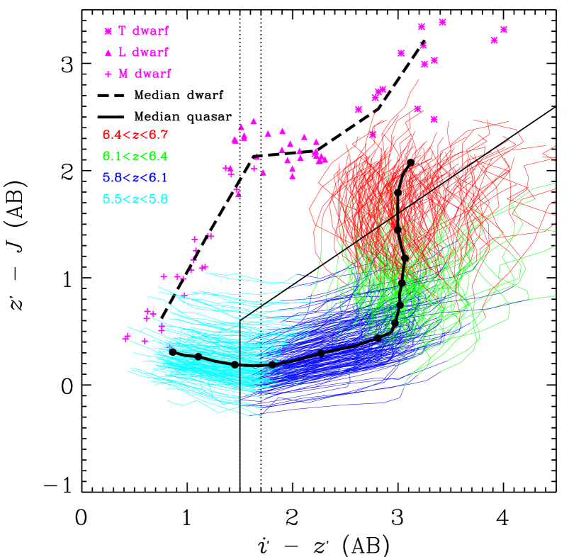
Figure 1.— $i^{\prime}-z^{\prime}$ vs $z^{\prime}-J$ in the CFHT filters for simulated quasars and literature low mass stars. The coloured curves show the tracks in colour-colour space of the 180 redshifted $z\sim 3$ quasars as they are moved from $z=5.5$ at lower-left to $z=6.7$ at upper-right (Sec. 2.1). The median colours at each redshift are calculated to produce the median quasar track (thick black line). Intervals of $\delta z=0.1$ along this track are marked with circles. The $i^{\prime}-z^{\prime}$ vs $z^{\prime}-J$ colours of low mass stars from the literature are shown as plus signs (M dwarfs), triangles (L dwarfs), asterisks (T dwarfs) (Sec. 2.2). The median star colours as a function of type are shown with a thick dashed line. The thin solid line denotes the high-redshift quasar selection region given in eqns. 1 and 2. Dotted lines indicate $i^{\prime}-z^{\prime}=1.5$ and $i^{\prime}-z^{\prime}=1.7$.

To determine the colours of quasars in our filters we convolve the 180 simulated quasar spectra with the $i^{\prime},z^{\prime}$ (MegaCam) and $J$ (CFHT-IR) filters. The filter profiles include the effect of CCD quantum efficiency and atmospheric transmission. All magnitudes are determined on the AB system. Note this is different from the $z>5.7$ quasar survey in the SDSS where $i^{\prime}$ and $z^{\prime}$ are on the AB system, but $J$ is on the Vega system. The colours are determined for a range of redshifts from $z=5.5$ to $z=6.7$. We also ran the simulated quasar spectra through the SDSS filter system to determine the SDSS colours of our quasar templates. We found good agreement between the simulated $i^{\prime}-z^{\prime}$ colours as a function of redshift and the observed colours of the 12 $z>5.7$ SDSS quasars. This provides a check on our Lyman forest absorption technique since the $i^{\prime}-z^{\prime}$ colours are particularly sensitive to this absorption.

The $i^{\prime}-z^{\prime}$ vs $z^{\prime}-J$ diagram is shown in Fig. 1. The colours of all 180 simulated quasars are plotted as a function of redshift from $z=5.5$ at lower-left to $z=6.7$ at upper-right. Note the tracks of the quasars in colour-colour space follow a similar trend to that shown for a simulated quasar in the SDSS system in Fan et al. (2003). However, there is a significant difference. The SDSS $i^{\prime}$ and $z^{\prime}$ filters are not overlapping, whereas there is a small, but significant, overlap for the MegaCam filters. The effect of this overlap is to decrease the $i^{\prime}-z^{\prime}$ colours of quasars, particularly in the range $5.7<z<6$ where the Ly $\alpha$ line passes through the overlap region. Therefore we need to adopt a lower $i^{\prime}-z^{\prime}$ selection criteria than the $i^{\prime}-z^{\prime}\geq 2.2$ used by the SDSS if we are to select quasars at similar redshifts. The box bounded by the regions

$$i^{\prime}-z^{\prime}\geq 1.5$$ (1)

$$i^{\prime}-z^{\prime}-1.5(z^{\prime}-J)\geq 0.6$$ (2)

defines the default colour-colour high-redshift quasar selection criteria. It can be seen from inspection of the figure that these criteria select almost all quasars in the range $5.8<z<6.4$.

Figure 2.— The fraction of quasars selected by the colour selection criteria of eqns. 1 and 2 as a function of redshift (solid line). This takes into account photometric scatter as described in Sec. 2.1. The dashed and dotted lines show the fractions if replacing eqn. 1 with $i^{\prime}-z^{\prime}\geq 1.6$ and 1.7, respectively.

To determine the quasar selection efficiency as a function of redshift more quantitatively, we have determined the fraction of quasars as a function of redshift which fall within this box. To account for the fact that the colours of objects detected in CCD imaging have a photometric uncertainty we model the location of each quasar at each redshift in colour-colour space as a 2D gaussian probability density distribution with $\sigma=0.2$. This error in colours is typical for the faintest sources in our survey (Sec. 3.2). We then proceed to calculate the fraction of the probability that falls within the selection region. This process is repeated for three different $i^{\prime}-z^{\prime}$ cuts of $1.5,1.6$ and $1.7$ to determine the effect of imposing different colour cuts on the selection efficiency as a function of redshift.

The results of this process are shown in Fig. 2. Quasars can be selected over the redshift range $5.7<z<6.5$ at a completeness fraction of $>0.5$. The completeness is close to unity at $5.8<z<6.4$. The effect of imposing a stricter cut of $i^{\prime}-z^{\prime}\geq 1.6$ or 1.7 is fairly small and only has an impact at the lower end of the redshift range (up to $z=5.9$).

2.2. Ultracool stars

To determine the colours of ultracool stars (M, L and T dwarfs) in our filters we convolve observed spectra obtained from Sandy Leggett’s online database with the $i^{\prime}$, $z^{\prime}$ (Mega Cam) and $J$ (CFHT-IR) filters. Only stars without significant gaps in spectral coverage at the wavelengths of these filters were used. The spectra are from the following sources: Tsvetanov et al. (2000), Burgasser et al. (2000), Kirkpatrick et al. (2000), Reid et al. (2001), Leggett et al. (2002) and Knapp et al. (2004). Fig. 1 shows the dwarf colours as plus signs (M), triangles (L) and asterisks (T). A sequence is also plotted by binning the dwarfs by type and evaluating the median colour in each bin. This figure demonstrates that the $i^{\prime}-z^{\prime}$ vs $z^{\prime}-J$ diagram provides a very clean separation between quasars and brown dwarfs for $i^{\prime}-z^{\prime}>$1.3. The $i^{\prime}-z^{\prime}\geq 1.5$ selection criteria which we adopt nominally selects dwarfs cooler than L2/L3. With significant noise in our colours and the much larger population of late-M dwarfs in a flux-limited sample, a significant number of slightly warmer stars may be observed to have $i^{\prime}-z^{\prime}\geq 1.5$.

3. Observations

3.1. CFHTLS Imaging

In this paper we use optical imaging from the Canada-France-Hawaii Telescope Legacy Survey (CFHTLS) to search for high-redshift quasars. The data used come from the first official release: T0001. This release includes data in the four Deep Survey fields obtained during the period June 2003 - July 2004. The Deep Survey has a 5-year lifetime, so the final dataset will go $\sim 1$ mag deeper than the data used in this paper.

Full details of this dataset are available elsewhere, but here we summarise the details relevant to our quasar search. Each of the four Deep fields (named D1-4) is one dithered pointing with the MegaCam camera. Therefore the total area of each field is $\approx 1$ sq. deg. The total integration time per field in the $i^{\prime}$ and $z^{\prime}$ filters respectively are D1: 52.0 ks, 12.2 ks; D2: 18.5 ks, 10.1 ks; D3: 59.6 ks, 15.1 ks; D4: 58.8 ks, 26.6 ks. The seeing FWHM is $\approx 0.9^{\prime\prime}$ in all the images. The astrometry of the images in the two bands are aligned to better than a pixel ($0.186^{\prime\prime}$).

To find very red objects in this dataset we generated catalogues of objects detected in the $z^{\prime}$-band images using the Sextractor software (Bertin & Arnouts 1996). We ran Sextractor in “double-image” mode to determine $i^{\prime}$-band measurements for all the objects detected in $z^{\prime}$. Magnitudes in both images were measured in $2^{\prime\prime}$ circular apertures. Aperture corrections to total magnitudes were applied for unresolved sources. The magnitudes have been corrected for galactic extinction using the maps of Schlegel, Finkbeiner & Davis (1998). Note that stars may not lie behind the total galactic obscuring column, but since the main goal of this paper is quasar selection and the applied galactic extinction corrections are smaller than our photometric errors, we do not attempt any further corrections for stars.

From these catalogues we drew a sample of objects satisfying the colour criterion of eqn. 1. We restricted the selection to sources which have $z^{\prime}$-band photometric errors $\sigma(z^{\prime})\leq 0.10$ to ensure we do not spend time following up spurious detections. Although images of these fields in the $u^{*},g^{\prime}$ and $r^{\prime}$ filters are also part of the T0001 release, we did not impose any other colour criteria since the $i^{\prime}$ images have the longest integration time so most selected objects are undetected at shorter wavelengths. Every candidate was inspected by eye to ensure that it is real. There were many spurious sources, mostly located near to very bright stars, where the diffraction patterns in the $i^{\prime}$ and $z^{\prime}$ images were different. After excising these from our target list we are left with 7, 12, 11 and 5 objects satisfying eqn. 1 and $\sigma(z^{\prime})\leq 0.10$ in fields D1, D2, D3 and D4, respectively.

3.2. Near-infrared imaging

As shown for the SDSS by Fan et al. (2001) and discussed in Sec. 2, the most efficient way of discriminating between high-redshift quasars and brown dwarfs is by using near-infrared $J$-band photometry. Brown dwarfs and very low mass stars have red $z^{\prime}-J$ colours and quasars have blue $z^{\prime}-J$ colours. The exact colour selection criteria used in the CFHQS to separate stars and quasars was given in Sec. 2.1.

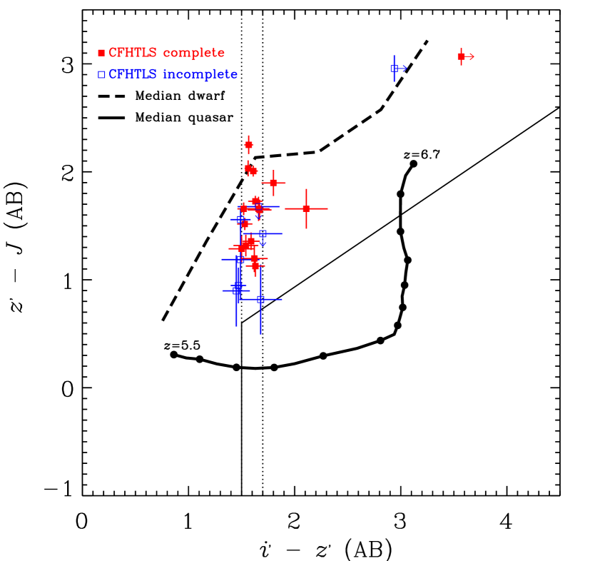
Figure 3.— Very red objects selected from the CFHTLS Deep $i^{\prime}$ and $z^{\prime}$ imaging which were observed with CFHT-IR at $J$-band are shown by squares with $1\sigma$ error bars. Filled squares show those objects belonging to the complete sample of candidates defined by $i^{\prime}-z^{\prime}\geq 1.5$, $\sigma(z^{\prime})\leq 0.10$ and $z^{\prime}<23.35$. Open squares show sources observed which fail one or more of these criteria. Also shown are the median colours of simulated quasars (thick solid line) and low mass stars (thick dashed line) from Fig. 1. The thin solid line denotes the high-redshift quasar selection region given in eqns. 1 and 2. Dotted lines indicate $i^{\prime}-z^{\prime}=1.5$ and $i^{\prime}-z^{\prime}=1.7$.

Table 1Table of observed objects.

Field	Name	$i^{\prime}$ (AB)	$z^{\prime}$ (AB)	$J$ (AB)	Complete?
D1	CFHTLS J022506.79-042958.4	$25.41\pm 0.18$	$23.30\pm 0.09$	$21.64\pm 0.16$	$\checkmark$
D1	CFHTLS J022456.72-045905.9	$24.30\pm 0.10$	$22.80\pm 0.07$	$21.51\pm 0.10$	$\checkmark$
D1	CFHTLS J022714.12-045723.1	$24.35\pm 0.10$	$22.81\pm 0.06$	$21.49\pm 0.08$	$\checkmark$
D1	CFHTLS J022455.66-040602.2	$21.78\pm 0.03$	$20.17\pm 0.03$	$18.16\pm 0.04$	$\checkmark$
D1	CFHTLS J022415.59-040431.1	$23.80\pm 0.07$	$22.21\pm 0.04$	$20.85\pm 0.07$	$\checkmark$
D1	CFHTLS J022559.39-040400.0	$23.47\pm 0.06$	$21.84\pm 0.03$	$20.11\pm 0.04$	$\checkmark$
D1	CFHTLS J022728.09-040318.7	$23.49\pm 0.06$	$21.96\pm 0.04$	$20.44\pm 0.04$	$\checkmark$
D2	CFHTLS J100113.06+022622.4	$>26.35$	$22.78\pm 0.07$	$19.71\pm 0.04$	$\checkmark$
D2	CFHTLS J100142.08+014931.8	$24.22\pm 0.10$	$22.55\pm 0.05$	$20.90\pm 0.08$	$\checkmark$
D2	CFHTLS J100130.42+015952.8	$24.10\pm 0.09$	$22.44\pm 0.05$	$20.78\pm 0.10$	$\checkmark$
D2	CFHTLS J095928.34+021819.8	$24.37\pm 0.11$	$22.75\pm 0.06$	$21.55\pm 0.11$	$\checkmark$
D2	CFHTLS J095922.77+020207.9	$23.71\pm 0.08$	$22.08\pm 0.04$	$20.95\pm 0.09$	$\checkmark$
D2	CFHTLS J100132.04+020022.4	$22.91\pm 0.05$	$21.39\pm 0.03$	$19.73\pm 0.05$	$\checkmark$
D3	CFHTLS J141659.91+521521.9	$23.89\pm 0.04$	$22.32\pm 0.03$	$20.07\pm 0.08$	$\checkmark$
D3	CFHTLS J141731.77+523920.4	$23.73\pm 0.04$	$22.17\pm 0.03$	$20.13\pm 0.07$	$\checkmark$
D4	CFHTLS J221705.05-172932.5	$24.47\pm 0.10$	$22.67\pm 0.05$	$20.77\pm 0.11$	$\checkmark$
D1	CFHTLS J022757.64-043019.5	$25.03\pm 0.16$	$23.35\pm 0.12$	$22.53\pm 0.30$	$\times$
D1	CFHTLS J022516.57-041402.9	$24.87\pm 0.14$	$23.38\pm 0.11$	$22.19\pm 0.35$	$\times$
D1	CFHTLS J022614.42-044600.4	$24.26\pm 0.10$	$22.81\pm 0.08$	$21.91\pm 0.32$	$\times$
D1	CFHTLS J022734.82-042438.7	$23.52\pm 0.06$	$22.05\pm 0.04$	$21.10\pm 0.16$	$\times$
D2	CFHTLS J095914.80+023655.2	$>26.35$	$23.41\pm 0.10$	$20.45\pm 0.07$	$\times$
D4	CFHTLS J221430.53-180230.5	$25.11\pm 0.16$	$23.41\pm 0.09$	$>21.98$	$\times$
D4	CFHTLS J221457.74-172104.2	$25.32\pm 0.17$	$23.66\pm 0.10$	$>21.98$	$\times$
D4	CFHTLS J221437.22-180417.4	$24.08\pm 0.08$	$22.59\pm 0.05$	$21.03\pm 0.09$	$\times$

Note. — Objects selected by their red $i^{\prime}-z^{\prime}$ colours from the CFHTLS Deep fields which were observed at $J$-band with CFHT-IR. The magnitudes listed are total magnitudes derived from aperture magnitudes. The final column indicates whether the object satisfies the $i^{\prime}$ and $z^{\prime}$ selection criteria which form the basis for our complete sample of quasar candidates for $J$-band imaging. These criteria are $i^{\prime}-z^{\prime}\geq 1.5$, $\sigma(z^{\prime})\leq 0.10$ and $z^{\prime}<23.35$. The three-colour photometry indicates that all these objects are ultracool dwarfs (Fig. 3). Their properties are discussed further in Sec. 3.3.

Observations at $J$-band were performed using the CFHT-IR camera at the CFHT. CFHT-IR is a HgCdTe $1024^{2}$ array with pixel size $0.211\,^{\prime\prime}$. Observations were carried out in photometric conditions on UT 2003 November 9, 10, 2004 May 4 and 2004 November 23, 24. Our first observations with CFHT-IR came a year before the T0001 release of the CFHTLS Deep data. For the first two observing runs we used preliminary reductions of the CFHTLS dataset generated by one of us (SDJG) and also by David Balam and Chris Pritchet. This led to the observation of some objects which now have $i^{\prime}-z^{\prime}<1.5$ in the most recent (and deepest) reduction. Due to constraints imposed by scheduling and poor weather it has not been possible to observe a complete sample of $i^{\prime}-z^{\prime}>1.5$ sources to a consistent magnitude limit in all 4 fields. We prioritised the reddest and brightest sources so that we can quantify our incompleteness. The sources not observed all lie close to the $i^{\prime}-z^{\prime}=1.5$ boundary and therefore we can account for the possibility they may be quasars at $z\approx 5.8$ in our selection function (Sec. 3.4).

A total of 24 sources were observed at $J$-band of which 20 have $i^{\prime}-z^{\prime}\geq 1.5$ (the rest have $1.45\leq i^{\prime}-z^{\prime}<1.5$). 15 out of the 35 sources identified in Sec. 3.1 were not observed (five in D2, nine in D3 and one in D4). The poor completeness in D3 is a consequence of bad weather during the CFHT-IR run in May 2004. $J$-band magnitudes on the AB scale were measured using $2^{\prime\prime}$ circular apertures and aperture corrections applied to give total magnitudes.

The resulting photometry is given in Table 1. The $i^{\prime}-z^{\prime}$ vs $z^{\prime}-J$ colours of these objects are plotted in Fig. 3. As is immediately clear in this diagram, the colours of all 24 targeted objects are consistent with stars and inconsistent with quasars. The three closest to the quasar selection region with $z^{\prime}-J<1$ are not part of the complete sample. Two of these have $i^{\prime}-z^{\prime}<1.5$. The other has $\sigma(z^{\prime})>0.10$ and a large uncertainty on its $J$-band magnitude and hence $z^{\prime}-J$ colour. It is possible that this object is a quasar, but given the poor constraint on its colour and the fact that stars are many times more common than quasars at this $i^{\prime}-z^{\prime}$ colour, the prior on the likelihood is that it is a star.

The two reddest objects (at $z^{\prime}-J\approx 3$) do lie close to the expected colours of $z>6.8$ quasars. However such a high redshift would require very high-luminosity quasars since at this redshift the Lyman-$\alpha$ line is moving out of the $z^{\prime}$-band. The luminosity of such quasars would be comparable to those in the SDSS at $z\sim 6$ which have a surface density of $\approx 1$ per 500 square degrees (Fan et al. 2004). The probability of finding such a quasar in 3.8 square degrees is very low. There is a much greater probability that they are T dwarfs (see Sec. 3.3). Even if these objects were quasars it would not affect the results of the rest of this paper because we only use the survey volume for quasars out to $z=6.4$.

3.3. Ultracool dwarfs detected

The two reddest objects (CFHTLS J095914.80+023655.2, $i^{\prime}-z^{\prime}>2.9$ and CFHTLS J100113.06+022622.4, $i^{\prime}-z^{\prime}>3.5$) both have $z^{\prime}-J\approx 3$ and are T dwarfs. The constraint from the $i^{\prime}-z^{\prime}$ and $z^{\prime}-J$ colours indicate that the former is cooler than T1 and the latter cooler than T4. To characterise their type more effectively we obtained $H$-band photometry of them with CFHT-IR. Both objects are very blue at $J-H$ confirming their T dwarf nature (even bluer than a $z\sim 7$ quasar). CFHTLS J095914.80+023655.2 has $J-H({\rm AB})=-0.26\pm 0.09$ and CFHTLS J100113.06+022622.4 has $J-H({\rm AB})=-0.70\pm 0.08$. Using the transformation $J-H({\rm Vega})=J-H({\rm AB})+0.44$ for comparison with the plot of $J-H$ vs spectral type in Leggett et al. (2002), we find that CFHTLS J095914.80+023655.2 is type T3 and CFHTLS J100113.06+022622.4 is type T6. With J${}_{\rm AB}\approx 20$, they are $3-4$ magnitudes fainter than most SDSS and 2MASS T dwarfs. Approximate distances based upon the relationship between absolute magnitude and spectral type (Tinney, Burgasser and Kirkpatrick 2003) are 150 and 70 pc, respectively, making them two of the most distant T dwarfs known.

Only four or five of the analysed objects have colours typical of L dwarfs ($i^{\prime}-z^{\prime}>1.5$ and $z^{\prime}-J\sim 2.0$). The $z^{\prime}-J<1.7$ colours of the rest indicate that they are late-M dwarfs, with a true $i^{\prime}-z^{\prime}$ below 1.5, scattered into our $i^{\prime}-z^{\prime}$ box by 1-3 $\sigma$ random noise excursions (this scattering is also apparent in the SDSS sample, see e.g., Fig. 3 of Fan et al. 2003). Within the limited statistics, the number of detected L dwarfs is consistent with an extrapolation of the densities seen in the shallow whole sky surveys.

3.4. Completeness

To turn the non-detection of quasars in this dataset into a useful limit on the quasar space-density and luminosity function, it is necessary to evaluate the completeness of our survey. There are two relevant selection criteria which will affect the completeness as a function of redshift and absolute magnitude:

• The $z^{\prime}$-band magnitude limit as a function of the survey area

• The colour selection criteria

Excluding the field edges which we have masked out of our catalogues, the $z^{\prime}$-band images show a fairly uniform noise and therefore detection limit across the field. Since the majority of our candidates have $z^{\prime}<23.35$ and point-sources of this magnitude have $\sigma(z^{\prime})\leq 0.10$  across most of the survey, we adopt a magnitude limit for the present analysis of $z^{\prime}<23.35$. To determine the efficiency with which objects could be found as a function of magnitude we ran simulations by inserting 10 000 artificial stars into each $z^{\prime}$-band image and using Sextractor to recover them. Even at bright magnitudes, about 5% of sources are not recovered because they overlap with other objects or regions affected by bright stars. We note that this fraction is much lower than the $\approx 20\%$ of the area in the mask region file released by Terapix. We find their masking to be much too conservative for our purpose. By $z^{\prime}=23.5$ the recovered fraction has decreased to $\approx 80\%$ in all the images. For each field we determine the area in which sources can be found as a function of their magnitude. At bright magnitudes the total area surveyed is 3.83 sq deg, dropping to 3.32 sq deg. at our limit of $z^{\prime}=23.35$.

The colour selection criteria were discussed extensively with simulated quasar and stellar colours in Sec. 2.1. Here we recap these selection criteria and evaluate the extent to which colour selection impacts our completeness. The nominal colour selection criteria are $i^{\prime}-z^{\prime}\geq 1.5$ and $i^{\prime}-z^{\prime}-1.5(z^{\prime}-J)\geq 0.6$. No observed objects lie within this box. Since we were unable to observe all the candidates with $i^{\prime}-z^{\prime}>1.5$ down to the magnitude limit, our completeness level in terms of the $i^{\prime}-z^{\prime}$ colour varies from field-to-field. Field D1 is complete to $i^{\prime}-z^{\prime}\geq 1.5$, D2 and D3 are complete to $i^{\prime}-z^{\prime}\geq 1.7$ and D4 is complete to $i^{\prime}-z^{\prime}\geq 1.6$. Note that even though only two out of eleven candidates in D3 were observed, all the unobserved objects have $1.5\leq i^{\prime}-z^{\prime}<1.7$.

Fig. 2 showed the completeness due to colour cuts as determined from the simulated high-redshift quasar colours. The effect of implementing redder cuts than the nominal $i^{\prime}-z^{\prime}\geq 1.5$ is to exclude quasars in the range $5.7<z<5.9$. The completeness at $z=5.8$ is $89\%,80\%$ and $68\%$ for $i^{\prime}-z^{\prime}\geq 1.5,1.6$ and $1.7$, respectively. At $z=5.9$, the colour completeness for all three cuts are $>98\%$. Therefore using a redder cut in $i^{\prime}-z^{\prime}$ makes only a very small difference to our sensitivity to quasars across the full range of $5.8<z<6.4$. This means that we can include fields like D2 and D3 which have not been so well followed up in the near-infrared whilst losing only a small amount in the completeness of high-redshift quasar selection.

The magnitude and colour completenesses are combined to generate an effective volume of our high-redshift quasar survey as a function of redshift (over the interval $5.8<z<6.4$) and absolute magnitude. Absolute magnitudes of the quasar continuum at a rest-frame wavelength of 1450Å are calculated for the possible range of apparent $z^{\prime}$-band magnitudes. These calculations use $k$-corrections generated from the mean $k$-corrections of the 180 redshifted $z\approx 3$ quasars discussed in Sec. 2.1.

4. Constraining the quasar luminosity function

We now use the non-detection of high-redshift quasars in the CFHTLS Deep fields to constrain the luminosity function (LF). We parametrise the LF using the double power-law form that provides a good fit at lower redshift (Croom et al. 2004), i.e.

$$\Phi(M_{1450},z)=\frac{\Phi(M_{1450}^{*})}{10^{0.4(\alpha+1)(M_{1450}-M_{1450}^{*})}+10^{0.4(\beta+1)(M_{1450}-M_{1450}^{*})}}.$$ (3)

The luminosity distribution of SDSS $z\approx 6$ quasars from Fan et al. (2004) is used to fit the bright-end normalisation $\Phi(M_{1450}=-26)$ as a function of the bright-end slope $\beta$. Taking the range in $\beta$ allowed by the SDSS and the value of $\Phi(M_{1450}=-26)$ at each $\beta$, we set up an array of possible double-power-law LFs. The faint-end slope $\alpha$ will not be strongly constrained by our data and therefore we do not treat this as a free parameter. Instead we assume that $\alpha$ takes a value of $-1.0,-1.5$ or $-2.0$ and repeat our analysis for each of these values. The best-fit values at the highest redshifts at which $\alpha$ has been measured ($z\sim 2-3$) lie in the range $-1.1$ to $-1.8$ (Boyle et al. 2000; Croom et al. 2004; Hunt et al. 2004; Richards et al. 2005). We will consider the effect of $\alpha$ later on. Sec. 3.4 discussed our survey volume as a function of redshift and absolute magnitude. We use the array of possible LFs combined with the survey volume to calculate the number of $5.8<z<6.4$ quasars $\mu$ that we would expect to have discovered in our survey as a function of $\beta$ and break magnitude $M^{*}_{1450}$. The probability of not finding any quasars given this LF is then simply given by the Poisson probability $P=e^{-\mu}$.

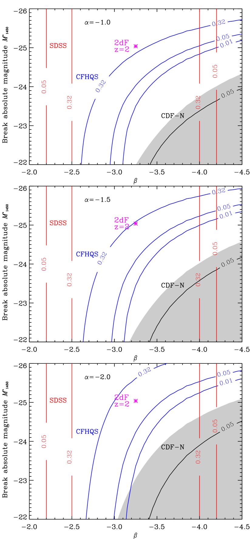
Figure 4.— Constraints on the $z=6$ quasar luminosity function from a variety of optical surveys. Each panel shows the constraints on the bright-end slope $\beta$ and break magnitude $M^{*}_{1450}$. The three panels assume values for the faint-end slope of $\alpha=-1$ (upper), $-1.5$ (middle) and $-2$ (lower). Confidence intervals are drawn for the CFHQS, SDSS and the CDF-N (Sec. 4). The best fit parameter values for the 2dF at $z=2$ (Croom et al. 2004) are shown for reference. The grey shaded region shows the values of parameters necessary for the $z=6$ quasar population to produce enough ionizing photons to reionize the universe as described in Sec 5.

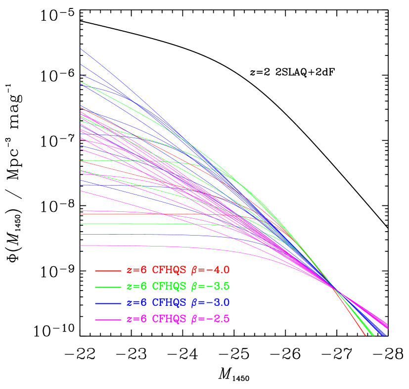
Figure 5.— Plausible double power-law parametrisations of the $z=6$ quasar optical luminosity function are shown as colored lines. Only those models with confidence levels $\geq 0.05$ based on the CFHQS and SDSS constraints are shown. These models are normalized to the SDSS results of Fan et al. (2004) which is why they have approximately the same density at $M_{1450}=-27$. The luminosity function at $z=2$ from the 2SLAQ + 2dF surveys (Richards et al. 2005) is shown as a black line. Our work finds that the large decrease in the space density of luminous quasars from $z=2$ to $z=6$ found by the SDSS also extends to lower luminosities ($M_{1450}\sim-24$).

The result of this analysis is shown in Fig. 4. Curves are plotted at confidence levels of $0.32,0.05$ and $0.01$. Separate panels show the different results obtained by assuming faint-end slopes of $\alpha=-1,-1.5,-2$. Since our survey is only sensitive to quasars brighter than $M_{1450}=-23$, our constraints depend weakly on $\alpha$ unless the break magnitude is very bright ($M^{*}_{1450}<-25$). The evolution in the 2dF quasar LF is fit by pure-luminosity evolution with the break evolving from $M^{*}_{1450}=-21$ at $z=0$ to $M^{*}_{1450}=-25$ at $z=2$ (Croom et al. 2004). Since the number density of luminous optically-selected quasars declines at redshifts beyond $2-3$ (Fan et al. 2004), continued pure-luminosity evolution would lead to a fainter $M^{*}_{1450}$ at $z=6$ than at $z=2$. Meiksin (2005) determined that a model with continued pure-luminosity evolution that fits the luminous SDSS $z=6$ sample would have $M^{*}_{1450}=-22.9$ at $z=6.0$. Although we do not necessarily expect the high-redshift evolution to be characterised by luminosity evolution, it is unlikely that the break magnitude would be brighter than it is at $z=2$, so we consider $M^{*}_{1450}=-25$ as a likely lower limit.

Barger et al. (2003) reported a negative search for $z>5.2$ quasars in the Chandra Deep Field-North (CDF-N). Their work goes deeper than our study (to $z^{\prime}=25.2$) but covers a much smaller area (0.031 sq. deg). We have therefore repeated our analysis of LF constraints using the lack of $5.8<z<6.4$ quasars in the CDF-N. The 0.05 confidence contour on $\beta$ and $M^{*}_{1450}$ from the CDF-N is plotted on Fig. 4. It can be seen that our constraint from CFHQS is considerably stronger than that from the CDF-N due to our survey volume being $\approx 100$ times greater. Also plotted on Fig. 4 are the constraints on $\beta$ from the luminosity distribution of the SDSS (Fan et al. 2004). The CFHQS provides much better lower limits on $\beta$ than the SDSS. For all the values of $\alpha$ considered, the 0.05 confidence limit is $\beta>-3.2$ if $M^{*}_{1450}=-24$ and $\beta>-3.1$ if $M^{*}_{1450}=-23$.

Fig. 5 shows the LF constraints from the CFHQS more directly. The colored curves correspond to LF models which are allowed at $\geq 0.05$ confidence. We can use the constrained LF parameters to place an upper limit on the space-density of quasars at $z=6$ brighter than a certain absolute magnitude limit. We adopt a limit of $M_{1450}<-23.5$ since at this magnitude cut there is almost no dependence of the density upper limit on $\alpha,\beta$, or $M^{*}_{1450}$. We find that $\rho(M_{1450}<-23.5)<1.7\times 10^{-7}\,{\rm Mpc}^{-3}$ at 95% confidence. This limit is a factor of 25 lower than the density at $z=2$ measured in the 2SLAQ + 2dF surveys (Richards et al. 2005). This confirms that the decline in the space-density of luminous quasars at $z\sim 6$ (Fan et al. 2004) is mirrored by the lower luminosity population. A decline in the space-density of low luminosity quasars has been seen in the range $z\sim 3-5$ (Barger et al. 2003; Wolf et al. 2003; Cristiani et al. 2004; Sharp et al. 2004), but the large volume and faint magnitude limit of our survey extends this result to $z\sim 6$.

5. A limit on the quasar contribution to the ionizing background at $z\sim 6$

If the high-redshift quasar LF can be fit by a double power-law with a break at $M^{*}_{1450}\raisebox{-2.58334pt}{$\,\stackrel{{\scriptstyle\raisebox{-0.60275pt}{$\textstyle<$}}}{{\sim}}\,$}-23$ and $\alpha>-2$, then a large fraction of the luminosity emitted by the quasar population will be emitted by quasars that we could have found in our survey. This means that our survey is useful for providing an upper limit to the number density of ionizing photons emitted by quasars at $z=6$.

To estimate the number of hydrogen-ionizing photons emitted by a quasar with a given $M_{1450}$, we assume the typical spectral shape determined for a large sample of quasars by Telfer et al. (2002). We assume that 100% of these photons escape from the host galaxy. The ionizing photon emission density is calculated by multiplying the photon emission rate per quasar by the number density of quasars and integrating over the range of quasar luminosities. We perform the integration down to quasars as faint as $M_{1450}=-18$.

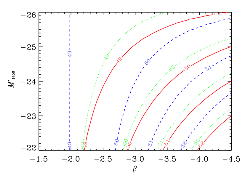
Figure 6.— The ionizing photon production rate density for the $z=6$ quasar population as a function of $\beta$ and $M^{*}_{1450}$. Contours are drawn for three values of the luminosity function faint-end slope: $\alpha=-1$ (solid), $-1.5$ (dotted) and $-2$ (dashed). Contours are plotted at $10^{49},10^{50},10^{51},10^{52}$ photons s^-1 Mpc^-3.

Fig. 6 shows the ionizing photon production rate density for the $z=6$ quasar population as a function of $\beta$ and $M^{*}_{1450}$. Contours are plotted for the three different values of $\alpha$ considered in the previous section. Note that the shape of the contours is quite similar to the shape of the confidence limits on these parameters determined from our survey for high-redshift quasars. This is due to the reason outlined previously that the main constraint from our survey is on the number density of quasars brighter than $M_{1450}=-23$ and such quasars dominate the ionizing photon budget unless $\alpha$ is very steep. We note that the ionizing photon production rate density in Fig. 6 is consistent with the calculations of Fan et al. (2001), but not with those of Yan & Windhorst (2004) who found a factor of 10 lower rate for the same quasar LF parameters. The reason for this discrepancy is unclear.

There is considerable debate about the photon density required to reionize the diffuse neutral hydrogen in the universe at $z=6$. The main uncertainty is due to recombination of ionized hydrogen atoms, which depends upon the clumpiness of the IGM. A detailed discussion of the clumpiness issue is beyond the scope of this paper. We follow Meiksin (2005) and assume that the clumpiness leads to 5 ionizing photons per hydrogen atom necessary for reionization at $z=6$. Note that this is substantially fewer than the 30 ionizing photons per hydrogen atom used by Madau et al. (1999) which has been widely used by other authors. Under our assumptions the ionizing photon production rate density necessary for reionizing the universe at $z=6$ is $3\times 10^{50}$ photons s^-1 Mpc^-3.

The region of $\beta-M^{*}_{1450}$ space where the quasar population alone can provide the necessary ionizing flux is shown by the grey shaded regions in Fig. 4. For any value of $\alpha$ the shaded region does not overlap with the CFHQS 0.05 confidence contours and quasars do not provide enough ionizing photons to reionize the universe. For $\alpha<-2$, the quasar emission is dominated by low luminosity quasars and a population with a break at $M^{*}_{1450}>-23$ could still reionize the universe, although the details then depend critically upon how far down the LF one integrates. All the evidence at intermediate redshifts points towards $\alpha\geq-1.8$ (Boyle et al. 2000; Croom et al. 2004; Hunt et al. 2004; Barger et al. 2005; Richards et al. 2005; but see Hao et al. 2005 for evidence that $\alpha\approx-2$ in the local universe) making it unlikely that $\alpha$ could be steeper than $-2$ at $z=6$. We conclude that a 95% confidence upper limit on the ionizing photon rate density provided by quasars at $z=6$ is $3\times 10^{50}$ photons s^-1 Mpc^-3.

6. Conclusions

We have used 3.83 sq. deg. of optical imaging with a magnitude limit of $z^{\prime}=23.35$ to search for high-redshift quasars. Near-infrared follow-up of candidates selected by their red $i^{\prime}-z^{\prime}$ colours all have $z^{\prime}-J$ colours consistent with being low mass stars: two are T dwarfs, four or five are L dwarfs, and the rest are late-M dwarfs scattered into our selection box by photometric errors.

The lack of quasars at $z>5.8$ in these data has been used to provide new constraints on the luminosity function. Several surveys underway at CFHT will image between $100-1000$ sq. deg. in multiple filters to somewhat shallower depths than the data in this paper. Assuming the bright-end slope is not much flatter than the value at $z=4$ of $\beta=-2.6$ (Fan et al. 2001), these surveys will allow the identification of many $z>5.8$ quasars giving a much more accurate determination of the luminosity function and provide targets for studying the ionization state of the IGM.

We have considered the ionizing photon output at $z=6$ and concluded that quasars provide $<3\times 10^{50}$ photons s^-1 Mpc^-3 at 95% confidence and assuming that the faint end slope $\alpha>-2$. The ionizing photon output from the $z\sim 6$ star-forming galaxy population is subject to significant uncertainties as outlined earlier, but the best estimates give a rate $\raisebox{-2.58334pt}{$\,\stackrel{{\scriptstyle\raisebox{-0.60275pt}{$\textstyle>$}}}{{\sim}}\,$}10^{51}$ photons s^-1 Mpc^-3 (Yan & Windhorst 2004; Bunker et al 2004; Stiavelli et al. 2004). Therefore quasars provide less than 30% as many ionizing photons as galaxies at $z\sim 6$. The evolution of the neutral hydrogen fraction inferred from quasar absorption spectra shows that the universe had been almost completely reionized by $z=6$ (Fan et al. 2004; Songaila 2004). Since something has to keep the universe reionized at this redshift, the most straightforward explanation is that the galaxy population is responsible.

References

- (1) Barger, A. J., Cowie, L. L., Capak, P., Alexander, D. M., Bauer, F. E., Brandt, W. N., Garmire, G. P., Hornschemeier, A. E. 2003, ApJ, 584, L61
- (2) Barger, A. J., Cowie, L. L., Mushotzky, R. F., Yang, Y., Wang, W.-H., Steffen, A. T., Capak, P. 2005, AJ, 129, 578
- (3) Barkana, R., Loeb, A. 2001, Phys. Rep., 349, 125
- (4) Bertin, E., Arnouts, S. 1996, A&AS, 117, 393
- (5) Boyle, B. J., Shanks, T., Croom, S. M., Smith, R. J., Miller, L., Loaring, N., Heymans, C. 2000, MNRAS, 317, 1014
- (6) Bouwens, R. J., et al. 2004, ApJ, 606L, 25
- (7) Bunker, A. J., Stanway, E. R., Ellis, R. S., McMahon, R. G. 2004, MNRAS, 355, 374
- (8) Burgasser A. J., et al. 2000, AJ, 120, 473
- (9) Chiu, K., et al. 2005, AJ, 130, 13
- (10) Comerford, J. M., Haiman, Z., Schaye, J. 2002, ApJ, 580, 63
- (11) Cristiani, S., et al. 2004, ApJ, 600L, 119
- (12) Croom, S. M., Smith, R. J., Boyle, B. J., Shanks, T., Miller, L., Outram, P. J., Loaring, N. S. 2004, MNRAS, 349, 1397
- (13) Dickinson, M., et al. 2004, ApJ, 600, L99
- (14) Dijkstra, M., Haiman, Z., Loeb, A. 2004, ApJ, 613, 646
- (15) Fan, X., et al. 2001, AJ, 122, 2833
- (16) Fan, X., et al. 2003, AJ, 125, 1649
- (17) Fan, X., et al. 2004, AJ, 128, 515
- (18) Haiman, Z., Abel, T., Madau, P. 2001, ApJ, 551, 599
- (19) Hao, L., et al. 2005, AJ, 129, 1795
- (20) Hunt, M. P., Steidel, C. S., Adelberger, K. L., Shapley, A. E. 2004, ApJ, 605, 625
- (21) Iliev, I. T., Shapiro, P. R., Raga, A. C. 2005, MNRAS, submitted, astro-ph/0408408
- (22) Kirkpatrick, J. D., et al. 2000, AJ, 120, 447
- (23) Knapp, G. R., et al. 2004, AJ, 127, 3553
- (24) Leggett, S. K., et al. 2002, ApJ, 564, 452
- (25) Madau, P., Haardt, F., Rees, M. J. 1999, ApJ, 514, 648
- (26) Madau, P., Rees, M. J., Volonteri, M., Haardt, F., Oh, S. P. 2004, ApJ, 604, 484
- (27) Meiksin, A. 2005, MNRAS, 356, 596
- (28) Oh, S. P., Haiman, Z. 2003, MNRAS, 346, 456
- (29) Reid, I. N., Burgasser, A. J., Cruz, K. L., Kirkpatrick, J. D., Gizis, J. E. 2001, AJ, 121, 1710
- (30) Richards, G. T., et al. 2002, AJ, 123, 2945
- (31) Richards, G. T., et al. 2004, AJ, 127, 1305
- (32) Richards, G. T., et al. 2005, MNRAS, 360, 839
- (33) Schlegel, D. J., Finkbeiner, D. P., Davis, M. 1998, ApJ, 500, 525
- (34) Sharp, R. G., Crampton, D., Hook, I. M., McMahon, R. G. 2004, MNRAS, 350, 449
- (35) Songaila, A. 2004, AJ, 127, 2598
- (36) Stiavelli, M., Fall, S. M., Panagia, N. 2004, ApJ, 610, L1
- (37) Telfer, R. C., Zheng, W., Kriss, G. A., Davidsen, A. F. 2002, ApJ, 565, 773
- (38) Tinney, C. G., Burgasser, A. J., Kirkpatrick, J. D. 2003, AJ, 126, 975
- (39) Tsvetanov, Z. I., et al. 2000, ApJ, 531, L61
- (40) Wolf, C., Wisotzki, L., Borch, A., Dye, S., Kleinheinrich, M., Meisenheimer, K. 2003, A&A, 408, 499
- (41) Wyithe, J. S. B., Loeb, A. 2002, ApJ, 577, 57
- (42) Wyithe, J. S. B. 2004, MNRAS, 351, 1266
- (43) Yan, H., Windhorst, R. A. 2004, ApJ, 600, L1