A fast method for computing strong-lensing cross sections: Application to merging clusters

Strong gravitational lensing by irregular mass distributions, such as galaxy clusters, is generally not well quantified by cross sections of analytic mass models. Computationally expensive ray-tracing methods have so far been necessary for accurate cross-section calculations. We describe a fast, semi-analytic method here which is based on surface integrals over high-magnification regions in the lens plane and demonstrate that it yields reliable cross sections even for complex, asymmetric mass distributions. The method is faster than ray-tracing simulations by factors of $\sim 30$ and thus suitable for large cosmological simulations, saving large amounts of computing time. We apply this method to a sample of galaxy cluster-sized dark matter haloes with simulated merger trees and show that cluster mergers approximately double the strong-lensing optical depth for lens redshifts $z_{\mathrm{l}}\gtrsim 0.5$ and sources near $z_{\mathrm{s}}=2$. We believe that this result hints at one possibility for understanding the recently detected high arcs abundance in clusters at moderate and high redshifts, and is thus worth further studies.

1 Introduction

Strong gravitational lensing by galaxy clusters is a highly non-linear effect which is very sensitive to the details of the lensing mass distribution. The cluster core densities, the asymmetries of their mass distribution, their substructures and their close neighbourhood all contribute to their lensing properties. The ongoing debate about whether the observed statistics of arcs is or is not compatible with the expectations in the standard $\Lambda$CDM cosmology shows that it is not sufficiently understood yet what aspects of the source and cluster populations as a whole determines the statistics of its strong-lensing effects (Bartelmann et al., 1998; Meneghetti et al., 2000, 2003b, 2003a; Wambsganss et al., 2004; Dalal et al., 2004; Li et al., 2005; Hennawi et al., 2005).

It is an obstacle for theoretical as well as observational studies that cross sections of galaxy clusters for strong lensing are costly to compute. So far, they require highly-resolved simulations tracing large numbers of light rays through realistically simulated cluster mass distributions, used for finding the images of sources which need to be classified automatically (Miralda-Escude, 1993; Bartelmann & Weiss, 1994). This needs to be done often, i.e. for different cosmological models and for many clusters in large cosmological volumes seen under many different angles, for the results to reach a reliable level. The recent finding that the enhanced tidal field around merging clusters substantially enhances strong-lensing cross sections (Torri et al., 2004) adds the necessity to study clusters with a time resolution which is sufficiently fine to resolve cluster merger events.

The increasing demands to be met by reliable strong-lensing calculations and the wish to carry them out for varying cosmological models calls for a substantially faster method than ray-tracing which should be equally reliable. We develop such a method here. It is based on the fact that highly elongated arcs occur near the critical curves in the lens plane, and that imaging properties near critical curves can be summarised by the eigenvalues of the Jacobian matrix of the lens mapping (see Schneider et al. (1992) and Sect. 2 for detail). This allows the reduction of the cross-section calculation to an area integral to be carried out on the lens plane itself. In that sense, the method is analytic, but the irregular shapes of the integration domains require it to be carried out numerically. Since the eigenvalues of the Jacobian matrix ideally describe imaging properties for infinitesimally small, circular sources, the method needs to be supplemented by techniques for taking extended, elliptical sources into account without losing computational speed.

The paper describes this method and its testing. After a brief summary of gravitational lensing in Sect. 2, we develop the new method and compare it to ray-tracing techniques in Sect. 3. We then describe in Sect. 4 its application to samples of cluster-sized halos whose evolution is described by merger trees. Results on cluster cross sections and optical depths are given in Sect. 5, and Sect. 6 provides summary and discussion.

2 Basic Gravitational Lensing

We briefly compile the basic equations of gravitational lensing necessary for quantifying the statistics of strong lensing events. Adopting the thin-lens approximation, the lensing mass distribution is projected perpendicular to the line of sight onto the lens plane, on which the physical coordinates $\@vec{\xi}=(\xi_{1},\xi_{2})$ are introduced. The coordinates on the source plane are $\@vec{\eta}=(\eta_{1},\eta_{2})$. Throughout this paper, we shall assume for simplicity that all sources are at the same redshift because their distribution in redshift is not relevant for developing our method. By means of the length scales $\xi_{0}$ and $\eta_{0}=(D_{\mathrm{s}}/D_{\mathrm{l}})\xi_{0}$ in the lens and source planes, respectively, we can introduce the dimension-less coordinates $\@vec{x}=\@vec{\xi}/\xi_{0}$ and $\@vec{y}=\@vec{\eta}/\eta_{0}$. The angular-diameter distances from the observer to the lens, the source, and from the lens to the source are $D_{\mathrm{l,s,ls}}$, respectively.

Source and image coordinates are related by the lens equation,

$$\@vec{y}=\@vec{x}-\@vec{\nabla}\psi(\@vec{x})=\@vec{x}-\@vec{\alpha}(\@vec{x})\;,$$ (1)

where $\@vec{\alpha}(\@vec{x})$ is the deflection angle, which is the gradient of the scalar lensing potential $\psi(\@vec{x})$ (see, e.g. Schneider et al. 1992). The Poisson equation

$$\Delta\psi(\@vec{x})=2\kappa(\@vec{x})=2\frac{\Sigma(\@vec{x})}{\Sigma_{\mathrm{cr}}}$$ (2)

relates the lensing potential to the (dimension-less) convergence $\kappa$, which is the surface-mass density $\Sigma$ in units of its critical value $\Sigma_{\mathrm{cr}}$.

The lens equation (1) defines a mapping from the lens to the source plane whose Jacobian matrix $\mathcal{A}(\@vec{x})$ describes how the shape of an infinitesimal source located at position $\@vec{y}$ is changed by the lens. It can be decomposed as

$$\mathcal{A}=\left(\begin{array}[]{cc}1-\kappa-\gamma_{1}&-\gamma_{2}\\ -\gamma_{2}&1-\kappa+\gamma_{1}\\ \end{array}\right)\;,$$ (3)

where the shear components $\gamma_{1,2}$ form a trace-less tensor quantifying the lensing distortion. The magnification of an image relative to the source is given by the inverse Jacobian determinant,

$$\mu(\@vec{x})=\frac{1}{\det\mathcal{A}(\@vec{x})}=\frac{1}{[1-\kappa(\@vec{x})]^{2}-\gamma_{1}^{2}(\@vec{x})-\gamma_{2}^{2}(\@vec{x})}\;.$$ (4)

Since the deflection angle is a gradient field, $\mathcal{A}(\@vec{x})$ is symmetric at any point on the lens plane (at least in the single-plane approximation which we are considering here), thus a coordinate rotation can always be found which diagonalises $\mathcal{A}$. Its two eigenvalues

$$\lambda_{\mathrm{t}}\equiv 1-\kappa-\gamma\;,\quad\lambda_{\mathrm{r}}\equiv 1-\kappa+\gamma$$ (5)

describe the distortion of an infinitesimal source in the tangential and radial directions relative to the lens’ centre and are thus called tangential and radial eigenvalues. At points in the lens plane where at least one of these two eigenvalues vanishes, the lens mapping becomes singular, yielding formally infinite magnifications for point sources. The set of all such points forms closed curves on the lens plane, the critical curves, whose images in the source plane are the caustic curves or caustics.

The central quantity describing the statistics of strongly distorted images with properties $p$ is the lensing cross section $\sigma_{p}$, defined as the area of the region on the source plane where a source with given characteristics has to lie in order to produce at least one image with properties $p$. The rest of this paper deals with images having length-to-width ratios exceeding a fixed threshold $d$. The respective cross section will be denoted as $\sigma_{d}$.

This lensing cross section quantifies the probability for a set of sources to be lensed by a given matter distribution into pronounced arc-like images. If we want to know how many arcs are expected to form on the entire sky (that is what we observe or can extrapolate from observations), we must sum the cross sections of all individual suitable lensing masses between us and the source plane, and then allow for variations of the source redshift. The lensing optical depth for sources at redshift $z_{\mathrm{s}}$ is

$$\tau_{d}(z_{\mathrm{s}})=\frac{1}{4\pi D_{\mathrm{s}}^{2}}\,\int_{0}^{z_{\mathrm{s}}}\int_{0}^{\infty}\,N(M,z)\,\sigma_{d}(M,z)\,\mathrm{d}M\mathrm{d}z\;,$$ (6)

where $N(M,z)dz$ is the total number of masses $M$ contained in the shell between redshifts $z$ and $z+\mathrm{d}z$. Denoting the differential mass function by $n(M,z)$ (Press & Schechter, 1974; Bond et al., 1991; Lacey & Cole, 1993, 1994; Sheth & Tormen, 1999, 2002) and the cosmic volume enclosed by a sphere of “radius” $z$ by $V(z)$, we can write

$$N(M,z)=\left|\frac{\mathrm{d}V(z)}{\mathrm{d}z}\right|\,n(M,z)\;.$$ (7)

If the number of sources with redshift between $z_{\mathrm{s}}$ and $z_{\mathrm{s}}+\mathrm{d}z_{\mathrm{s}}$ is $n_{\mathrm{s}}(z_{\mathrm{s}})\mathrm{d}z_{\mathrm{s}}$, the total number of gravitational arcs is

$$N_{d}=\int_{0}^{\infty}\,n_{\mathrm{s}}(z_{\mathrm{s}})\,\tau_{d}(z_{\mathrm{s}})\,\mathrm{d}z_{\mathrm{s}}\;.$$ (8)

In particular, if all sources are at the same redshift $z_{\mathrm{s}}$, the previous equation reduces to

$$N_{d}=n_{\mathrm{s}}(z_{\mathrm{s}})\,\tau_{d}(z_{\mathrm{s}})\;.$$ (9)

It is important for our discussion that the lensing cross section $\sigma(M,z)$ of a single structure depends sensitively on the source distribution and on the internal properties of the structure itself, in particular the slope of the inner density profile, the lumpiness and the asymmetries of the matter distribution (Bartelmann et al., 1995, 1998; Meneghetti et al., 2003b). These peculiarities of galaxy clusters are intimately linked with the formation and evolution histories of the respective dark-matter haloes, which in turn depend on cosmology (especially on the matter density parameter and the cosmological constant or dark energy). Moreover, the spatial volume per unit redshift, the source population and the cluster mass function also depend on cosmology (Lacey & Cole, 1993).

Given the importance of asymmetries in cluster mass distributions it is not promising to search an analytic expression for the function $\sigma(M,z)$, unless we consider highly symmetric (and thus unrealistic, see Meneghetti et al. 2003b) lens models. The alternative that we shall discuss in the next subsections is to use numerical or semi-analytic algorithms for calculating the lensing cross section of a set of model clusters that appropriately sample the mass and redshift range under consideration.

3 Lensing Cross Sections

So far, the most reliable method for calculating cross sections for long and thin arcs has been using fully numerical ray-tracing simulations. If performed adequately, such simulations return realistic cross sections, but with the disadvantage of being very expensive in terms of computational time. In view of cosmological applications, the mass and redshift ranges to be covered are large, in particular because the temporal sampling needs to be dense for properly resolving cluster merger events. The number of cross sections to be calculated can thus be very large. A reliable alternative to the costly ray-tracing simulations is therefore needed. We develop here a semi-analytic method which fairly reproduces fully numerical lensing cross sections, but at a computational cost which is lowered by factors of $\sim 30$. We believe this method to provide an elegant alternative to ray-tracing simulations for many applications of lensing statistics.

In the following subsections, we shall first describe the fully numerical method for reference, and then the semi-analytic method.

3.1 Ray-Tracing Simulations

Given the lensing mass distribution (which can be given as either an analytic density profile or a simulated density map) and the statistical properties of the source sample, strong-lensing cross sections are commonly estimated using fully numerical ray-tracing simulations. The method we use here was first described by Miralda-Escude (1993) and subsequently further developed and adapted to asymmetric, numerical lens models by Bartelmann & Weiss (1994). It has been widely used by Meneghetti et al. (2000, 2003b) and with several modifications by Puchwein et al. (2005). We only address its principal features here, referring the interested reader to the cited papers and the references given therein for further detail.

Briefly, a bundle of $n\times n$ light rays ($n=2048$ here) with an opening angle $\beta$ is sent from the observer through the lens. The opening angle depends on the lens’ properties and the distances involved, and must be large enough to encompass the entire region on the lens plane where strong lensing events may occur. The deflection angle is calculated from the surface-mass distribution at all points where light rays intersect the lens plane, thus allowing each ray to be propagated back to the source plane by means of the lens equation (1).

A set of sources is then placed on a regular and adaptive grid on the source plane. The sources are modelled as ellipses whose orientation angles and axis ratios (minor to major) are randomly drawn from the intervals $[0,\pi]$ and $[0.5,1]$, respectively, with the prescription each source has the area of a circle with $1$ arc second diameter. The source-grid resolution is iteratively increased near the caustics, i.e. where the magnification on the source plane is highest and undergoes rapid variations. This artificial increase in the probability of strong lensing events, must be corrected when calculating cross sections. We do so by assigning a statistical weight to each source which is proportional to the area of the grid cell which it represents.

The images of each source are found by identifying all rays of the bundle falling into the source. Simple geometrical shapes (ellipses, rectangles, and rings) are then fit to all images, and their characteristics (length, width, curvature radius, etc.) are determined. When an image has the property we are interested in (i.e. a length-to-width ratio equal to or greater than $d$), we increment the cross section by the pixel area of the source grid, times its statistical weight.

3.2 Semi-Analytic Method

3.2.1 Point Sources

We aim at determining cross sections for the formation of gravitational arcs with length-to-width ratio exceeding some fixed threshold $d$. Initially assuming infinitesimal (or point-like) sources, the discussion in Sect. 2 implies that such arcs will form where the ratio

$$R(\@vec{x})\equiv\max\left[\left|\frac{\lambda_{\mathrm{r}}(\@vec{x})}{\lambda_{\mathrm{t}}(\@vec{x})}\right|,\left|\frac{\lambda_{\mathrm{t}}(\@vec{x})}{\lambda_{\mathrm{r}}(\@vec{x})}\right|\right]$$ (10)

between the eigenvalues of the lens mapping satisfies

$$R(\@vec{x})\geq d\;.$$ (11)

We denote this region by $B_{l}=B_{l}(d)$. By means of the lens equation, $B_{l}$ can be mapped onto an equivalent region $B_{s}=B_{s}(d)$ on the source plane, whose area is by definition (see again Sect. 2) the cross section $\sigma_{d}$ we are searching for. Thus,

$$\sigma_{d}=\int_{B_{s}}\mathrm{d}^{2}\eta=\eta_{0}^{2}\int_{B_{s}}\mathrm{d}^{2}y\;.$$ (12)

The lens equation maps the infinitesimal area element on the lens plane to that on the source plane by means of the Jacobian determinant $\det\mathcal{A}(\@vec{x})$, thus

$$\sigma_{d}=\eta_{0}^{2}\int_{B_{l}}|\det\mathcal{A}(\@vec{x})|\mathrm{d}^{2}x=\eta_{0}^{2}\int_{B_{l}}\frac{\mathrm{d}^{2}x}{|\mu(\@vec{x})|}\;,$$ (13)

where Eq. (4) was used.

3.2.2 Extended Circular Sources

Although this line of reasoning is exact, it fails in reproducing simulated cross sections, for it does not account for real sources (and also the sources used in ray-tracing simulations) not being point-like. Extended sources are much more likely to produce strongly distorted images than point-like sources, and their imaging properties will only be approximated by the eigenvalue ratio $R(\@vec{x})$. This implies that the integral in (13) has to be extended beyond the region $B_{l}$, because an extended source can produce a long and thin arc even if it is centred where the eigenvalue ratio is less than $d$.

Introducing extended sources into the framework just outlined, we wish to convolve the eigenvalue ratio $R(\@vec{x})$ on the lens plane with a suitable function to be determined which significantly differs from zero only on the image of an extended source. For consistency with ray-tracing simulations, we assume circular sources with radius $\zeta=0.5^{\prime\prime}$ for now. Effects of source ellipticities will be included later.

The obvious problem with this approach is that the properties of the image vary wildly across the lens plane, thus the convolution should use a function which rapidly changes shape and extent across the lens plane. We can avoid this problem by transferring the calculations to the source plane. We first introduce the eigenvalue ratio on the source plane. Since multiple points $\@vec{x}_{i}$ on the lens plane may be mapped onto a single point $\@vec{y}$ on the source plane, we define it as $\bar{R}(\@vec{y})\equiv\max\{R[\@vec{y}(\@vec{x}_{i})]\}$. This ratio $\bar{R}(\@vec{y})$ is then convolved with a function $g(\@vec{y})$ which differs significantly from zero only on the circular area covered by a source, which is the same everywhere on the source plane. Let the convolution in the source plane be $\bar{h}(\@vec{y})\equiv\bar{R}(\@vec{y})*g(\@vec{y})$, then we put $h(\@vec{x})=\bar{h}[\@vec{y}(\@vec{x})]$ to obtain the convolved function on the lens plane, as desired. Again, we need to take into account that single points on the source plane may be mapped on multiple points in the lens plane. Assigning $R(\@vec{x})$ to $\bar{R}[\@vec{y}(\@vec{x})]$ now sets the convolved length-to-width ratio equal on all image points, which is not exact, but a tolerable error. The problem is now reduced to carrying out the convolution $\bar{h}(\@vec{y})$, which is discussed in the Appendix. As described there, we speed up the convolution by approximating it by a simple multiplication after essentially assuming that the eigenvalues of the lens mapping and their ratio do not change significantly across a single source.

Finally, what form should be chosen for the function $g(\@vec{y})$? A two-dimensional Gaussian of width $\zeta$ may appear intuitive, but the ray-tracing simulations we use for reference do not adopt a surface-brightness profile for sources because they simply bundle all rays falling into the ellipse representing a source. Thus, a choice for $g$ consistent with the ray-tracing simulations is a step function with width $\zeta$,

$$g(\@vec{y})=\left\{\begin{array}[]{l}(\pi\zeta^{2})^{-1}\quad\mbox{where}\quad\@vec{y}^{T}\mathcal{B}\@vec{y}\leq 1\\ 0\quad\mbox{else}\\ \end{array}\right.\;,$$ (14)

where $\mathcal{B}$ is a matrix describing the shape of the source. Since we are only considering circular sources of radius $\zeta$, $\mathcal{B}$ has the form $\mathcal{B}=\mathcal{I}/\zeta^{2}$, where $\mathcal{I}$ is the unit matrix. The factor $(\pi\zeta^{2})^{-1}$ in (14) normalises $g(\@vec{y})$ to unity. Substituting $h(x)$ for $R(x)$, we can again apply Eq. (11) to obtain a new region $B_{l}$ that will now of course be larger than before.

3.2.3 Extended Elliptical Sources

We finally have to account for elliptical rather than circular sources. It is quite obvious and was shown by many authors (e.g. Bartelmann et al. 1995; Keeton 2001) that elliptical sources are more likely to produce strongly distorted images.

We adopt the simple and elegant formalism by Keeton (2001). He showed that an elliptical source at position $\@vec{y}(\@vec{x})$ with axis ratio $q_{s}=a/b=q_{s}[\@vec{y}(\@vec{x})]$ and orientation angle $\theta=\theta[\@vec{y}(\@vec{x})]$ is imaged as an allipse with an axis ratio of

$$q_{\mathrm{obs}}=\sqrt{\frac{T+\sqrt{T^{2}-4D}}{T-\sqrt{T^{2}-4D}}}$$ (15)

where $T$ and $D$ are the trace and the determinant of the matrix that describes the image ellipse. They can be expressed as functions of the intrinsic source properties and of the (convolved) lensing distortion:

$$T=h^{2}+q_{s}^{2}+(h^{2}-1)(q_{s}^{2}-1)\,\cos^{2}\theta\;,\quad D=h^{2}q_{s}^{2}\;.$$ (16)

Again, $h(x)$ can be replaced by $q_{\mathrm{obs}}$ to obtain a modification of the region $B_{l}$, again larger than before, whose area is now a close approximation to the cross section we seek to determine, accounting for extended and elliptical sources.

3.2.4 Comparison to Ray-Tracing

As a final step, we test the accuracy of our calculations and approximations, especially those concerning the replacement of the convolution by a multiplication (cf. the Appendix), by comparing lensing cross sections obtained with the semi-analytic method to their fully numerical counterparts obtained by ray-tracing. Since the main purpose of this work is to estimate the effects of cluster mergers, we compare the cross sections as they evolve while two dark matter haloes merge. The halos are modelled as NFW profiles (see Navarro et al. 1995, 1996, 1997; Cole & Lacey 1996) whose lensing potential is elliptically distorted to have ellipticity $e=0.3$ (see Sect. 4 for detail). The results of the comparison are shown in Fig. 1 for various masses, redshifts and thresholds $d$.

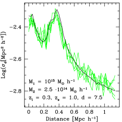
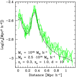
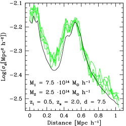
Figure 1: Lensing cross sections for long and thin arcs with length-to-width ratio exceeding $d$ as a function of the distance between the centres of two dark matter haloes, for two (lens and source) redshifts. The haloes are modelled as NFW density profiles with elliptically distorted lensing potential with ellipticity $e=0.3$ (see Sect. 4). Green lines show the results of ray-tracing simulations for five different realisations of the source distribution. Black lines are the results obtained with our semi-analytic method.

Figure 1 warrants one observation. The ray-tracing simulation was repeated five times for each modelled merger event, each time changing the seed for the random generation of source ellipticities and orientations. As the figure shows, this has quite a significant effect on the numerical cross sections, causing a substantial scatter. The reason can be easily understood. When a given source produces an arc, variations in the source’s intrinsic ellipticity and in the orientation with respect to the caustic structure can easily push the length-to-width ratio of the image arc below or above the chosen threshold $d$. This causes the irregular trend seen in Figure 1. It is worth noting that the same problem in principle also affects the semi-analytic results. In this case, however, ellipticity and orientation are assigned to each ray traced back through the lens plane simply to identify the the extended region over which we integrate. Since the number of rays is much larger than the number of individual sources used in the fully numerical algorithm, the random scatter in the semi-analytic results is very small. In fact, the fluctuations are of the order of the width of the black curve and thus omitted.

Moreover, it must be noted that the results given by the ray-tracing code we use might differ slightly from other codes using different resolution, different image finding algorithms and different ways to fit the image shapes.

Analysing Fig. 1, we can draw two interesting conclusions. The first is that, reassuringly, the numerical and the semi-analytic cross section agree excellently. This means that the approximations we made are substantially correct. There is, however, a small discrepancy for higher-redshift sources, shown in the lower panels. We believe that this discrepancy is due to the fact that the scale over which the lensing properties on the source plane change significantly is in this case comparable to the source dimension, thus one of the approximations we made in the Appendix fails, namely that the function $R[\@vec{y}(\@vec{x})]$ does not vary much across a source. Nonetheless, the discrepancy is nowhere larger than 20%, which is more than acceptable for our purposes, in particular in view of the considerable scatter in the ray-tracing results.

The second observation is that the behaviour of the cross sections (both numerical and semi-analytic) as a function of the distance between the haloes closely reflects that found by Torri et al. (2004). These authors studied the effect of a single merger process on the strong-lensing efficiency of a numerically simulated dark matter halo, using ray-tracing as described in Sect. 3. They found that, while the substructure is swallowed by the main halo, there is a first peak in the lensing cross section when the increasing shear field between the lumps causes the critical lines to merge, a local minimum while cusps disappear in the caustic branches, and another peak caused by the increased convergence when the two density profiles overlap. All these features are recovered in the panels of the Fig. 1.

This level of agreement between ray-tracing and semi-analytic cross sections show that the semi-analytic method developed above for cross-section calculations is essentially correct and constitutes a valid and useful, $\sim 30$ times faster alternative to the costly ray-tracing simulations.

4 Lensing Optical Depth

Given reliable lensing cross sections, lensing optical depths need to be determined following Eq. (6). For that purpose, we use the merger trees for a set of 46 numerically simulated dark-matter haloes, whose main properties are described in the next subsection. The merger tree of a dark-matter halo provides two types of information. First, we know how the mass of each halo evolves with time or redshift. Second, we know at which redshift merger events happen with substructures of known mass. Regarding this, it is worth recalling that the evolution of a dark-matter halo is characterised by the continuous accretion of infalling external material. We account for all mergers in which the main halo accretes a sub-haloes with at least 5% of the main halo’s mass. Nonetheless, it should be kept in mind that halos continuously accrete matter apart from merger events.

4.1 Halo Model

We base our study on the merger trees on a sample of 46 numerically simulated dark-matter haloes. These haloes were re-simulations at higher resolution of a large-scale cosmological simulation. The cosmological model used was a “concordance” $\Lambda$CDM model, having a cosmological constant of $\Omega_{\Lambda,0}=0.7$, a (dark) matter density of $\Omega_{\mathrm{m},0}=0.3$ and a Hubble constant of $h=0.7$. The power spectrum of the primordial density-fluctuation field is scale invariant (i.e. with a spectral index of $n=1$), and the rms linear density fluctuations on a comoving scale of $8\,h^{-1}\,\mathrm{Mpc}$ is $\sigma_{8}=0.9$, which is the typical value required to match the local abundance of massive galaxy clusters (White et al., 1993; Eke et al., 1996). The mass of dark-matter particles is $m=1.3\times 10^{9}\,h^{-1}\,M_{\odot}$. In Tab. 1 we list the present masses and virial radii for the three most massive and the tree least massive haloes in the sample.

Table 1: Present-day masses and virial radii for the three most massive and the three least massive haloes in our sample.

Halo Id.	Virial Mass	Virial Radius
	[$h^{-1}\,M_{\odot}$]	[$h^{-1}\,\mathrm{Mpc}$]
g8-a	2.289 $10^{15}$	2.146
g1-a	1.530 $10^{15}$	1.876
g72-a	1.374 $10^{15}$	1.810
g696-y	5.219 $10^{13}$	0.608
g696-z	5.171 $10^{13}$	0.607
g696-#	5.060 $10^{13}$	0.602

The present masses of the halo models vary between about $5\times 10^{13}\,h^{-1}\,M_{\odot}$ (just exceeding the mass of a massive cD galaxy) and more than $2\times 10^{15}\,h^{-1}\,M_{\odot}$, which is characteristic of a rich galaxy cluster.

We note in passing that, owing to the dependence of the cluster-evolution history on cosmology, the typical redshift of structure formation in the cosmological model used here is higher than in an Einstein-de Sitter universe, and lower than in an open low-density universe. Models of dark energy alternative to the cosmological constant typically shift this redshift towards higher redshifts, thus changing the contribution of cluster mergers to arc statistics. We are planning a future study to address this interesting property.

For describing specifically each individual merger process and its effects on gravitational-arc statistics, we model each dark-matter halo as NFW spheres. Their density profile is

$$\rho(r)=\frac{\rho_{\mathrm{s}}}{r/r_{\mathrm{s}}(1+r/r_{\mathrm{s}})^{2}}\;,$$ (17)

which fits the density profiles of numerically simulated dark-matter haloes and fairly describes dark structures over a wide range of masses and in different cosmologies. The scale density $\rho_{\mathrm{s}}$ and the scale radius $r_{\mathrm{s}}$ are linked by the halo concentration, $c=r_{200}/r_{\mathrm{s}}$, where $r_{200}$ is the radius enclosing a mean density of 200 times the closure density of the Universe. As a general trend, the concentration reflects the mean density of the Universe at the collapse redshift of the halo, thus it is higher for lower masses. Several ways to quantitatively relate the concentration to the halo mass have been proposed. We follow the prescription of Eke et al. (2001). The analytic fit (17) allows direct calculations of the main lensing properties. In particular, the projected density profile for a NFW lens is

$$\Sigma(x)=2\rho_{\mathrm{s}}r_{\mathrm{s}}\frac{f(x)}{x^{2}-1}\;,$$ (18)

and its deflection angle is

$$\alpha(x)=4\rho_{\mathrm{s}}r_{\mathrm{s}}\frac{g(x)}{x}\;,$$ (19)

where the functions $f(x)$ and $g(x)$ are

$$f(x) = \left\{\begin{array}[]{l}1-\frac{2}{\sqrt{x^{2}-1}}\arctan{\sqrt{\frac{x-1}{x+1}}}\quad\hbox{if}\quad x>1\\ 0\quad\hbox{if}\quad x=1\\ 1-\frac{2}{\sqrt{1-x^{2}}}\mbox{arctanh}{\sqrt{\frac{1-x}{1+x}}}\quad\mbox{else}\\ \end{array}\right.\;,$$ (23)

$$g(x) = \ln\frac{x}{2}+\left\{\begin{array}[]{l}\frac{2}{\sqrt{x^{2}-1}}\arctan{\sqrt{\frac{x-1}{x+1}}}\quad\mbox{if}\quad x>1\\ 1\quad\mbox{if}\quad x=1\\ \frac{2}{\sqrt{1-x^{2}}}\mbox{arctanh}{\sqrt{\frac{1-x}{1+x}}}\quad\mbox{else}\\ \end{array}\right.$$ (27)

(Bartelmann, 1996). Here and in the remainder of this sub-section, $x$ is the dimensionless distance from the lens’ centre. We additionally adopt elliptically distorted lensing potentials. Elliptical potentials are not equivalent to elliptical density distributions, but allow for much more straightforward calculations (Schneider et al., 1992), and the results are equally valid for our purposes (Golse & Kneib, 2002; Meneghetti et al., 2003b). In their work, Meneghetti et al. (2003b) also estimated the value of the ellipticity $e$ for the lensing potential that produces the best fit to the deflection-angle maps of simulated haloes. Following their result, we adopt $e=0.3$ throughout.

4.2 Modelling Halo Mergers

Once the redshift is fixed, the halo we consider may be isolated or in interaction with a substructure. In the first case the deflection angle can be obtained directly by means of equation (19). In the second, we can sum the deflection angles of the two structures at each point on the lens plane, owing to the linearity of the problem (Schneider et al., 1992; Torri et al., 2004). In both cases, the eigenvalues of the local mapping follow from the deflection-angle maps by differentiation, and can be applied in the semi-analytic method for calculating cross sections as described in Sect. 3.

Individual merger events are modelled as follows: The main halo and the substructure start at a mutual distance equal to the sum of their virial radii. Then the centres approach at a constant speed, calculated by the ratio of the initial distance to the typical time scale of a merger event, i.e. 0.9 Gyr (Torri et al., 2004; Tormen et al., 2004). The process is assumed to be concluded when the two density profiles overlap perfectly. The direction of approach, always assumed to be perpendicular to the observer’s line of sight, is parallel to the directions of the major axes of the lensing potential, which are also assumed to be parallel. This last assumption is well justified by recent work (Lee et al., 2005; Hopkins et al., 2005) pointing out, both with analytic models and numerical analyses, that there is an intrinsic alignment between a dark-matter halo and the surrounding haloes and sub-lumps due to the tidal field of the major halo itself. We note that assuming all mergers to proceed along directions perpendicular to the line-of-sight slightly underestimates the cumulative contribution of cluster mergers to the lensing optical depth, because if the merger direction is partially aligned with the line-of-sight, the time spent by the system in configurations leading to high cross sections is longer (see again Fig. 3). Several tests we made show however that this underestimation is typically of order 20%, thus we neglect it here.

Once we know for each halo at every redshift the cross section with and without the effect of mergers, we can compute lensing optical depths. Since we sample the mass range discretely, we cannot apply Eq. (6) directly, but need to approximate it as

$$\tau_{d}(z_{\mathrm{s}})=\int_{0}^{z_{\mathrm{s}}}\left[\sum_{i=1}^{n-1}\bar{\sigma}_{d,i}(z)\int_{M_{i}}^{M_{i+1}}N(M,z)\mathrm{d}M\right]\frac{\mathrm{d}z}{4\pi D_{\mathrm{s}}^{2}}\;,$$ (28)

where the masses $M_{i}$ ($1\leq i\neq n$) have to be sorted from the smallest to the largest at each redshift step, and the quantity $\bar{\sigma}_{d,i}(z)$ is defined as

$$\bar{\sigma}_{d,i}(z)=\frac{1}{2}\left[\sigma_{d}(M_{i},z)+\sigma_{d}(M_{i+1},z)\right]\;.$$ (29)

This is essentially equivalent to assigning to all structures with mass within $[M_{i},M_{i+1}]$ the average cross section of the haloes with masses $M_{i}$ and $M_{i+1}$, weighted with the number density of massive structures within that interval.

4.3 Mass Cut-Off

Since a sufficient condition for strong lensing is satisfied if the surface density of a lens exceeds the critical density somewhere, any lens model with a cuspy density profile such as the NFW profile will formally be a strong lens and thus produce critical curves and caustics. However, the caustics of low-mass halos will be smaller than the typical source galaxies. Averaging the local distortion due to a low-mass lens across an extended source will then lead to a small or negligible total distortion. This implies that the mass necessary for halos to cause large arcs is bounded from below by the requirement that the halo’s caustic must be sufficiently larger than the available sources.

This mass limit obviously depends on the lens and source redshifts due to the geometrical sensitivity of lensing. Higher masses are required at low and high redshifts for lensing effects comparable to lenses at intermediate redshifts. In addition, the caustic structures can change substantially during major halo mergers. As a sub-halo approaches the main halo, the initially separated caustics of the two merging components will increase and merge to form a larger caustic. Thus, even though the total mass is unchanged, the mass limit for strong lensing may decrease while a merger proceeds. Even halos which are individually not massive enough for arc formation may be pushed above the mass limit while they merge. In view of the exponentially dropping cluster mass function, this is potentially a huge effect.

Thus, we have to monitor the extent of the caustics as we compute the lensing optical depth of a halo sample, taking into account that the mass limit may change rapidly as halos merge with sub-halos. The lowest mass of a halo from our sample of 46 halos which still contributes to strong lensing is shown in Fig. 2 as a function of lens redshift with fixed source redshift $z_{\mathrm{s}}=2$.

Figure 2: Mass of the lowest-mass halo producing large arcs in the sample of 46 halos which we use here to compute the lensing optical depth. The source redshift is $z_{\mathrm{s}}=2$. The overall trend in the curve reflects the geometrical lensing sensitivity, while the fluctuations and the depth of the minimum reflect that mergers can lift low-mass halos above the strong-lensing threshold which would otherwise not be capable of strong lensing.

Following these prescriptions, we are able to calculate the strong-lensing cross section of each model halo at every redshift step of the simulation, first ignoring the effects of merger processes, then accounting for them. Thus, we sort the masses from the smallest to the largest at every redshift step and calculate the quantities $\sigma_{d,i}(z)$. Finally, we calculate the lensing optical depth with and without the effect of merger processes.

5 Results

5.1 Cross Sections

We calculate the optical depth for the formation of gravitational arcs with length-to-width ratio grater than an arbitrary threshold $d$. We used two choices, $d=7.5$ and $d=10$.

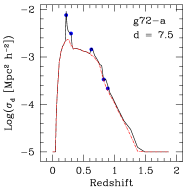
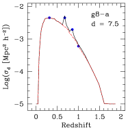
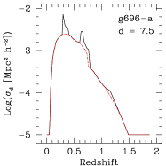
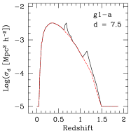
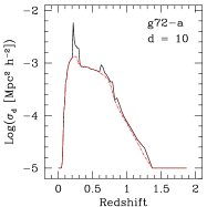
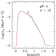
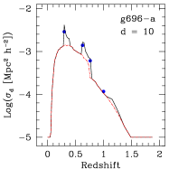
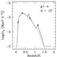
Figure 3: Evolution of the lensing cross section for gravitational arcs with length-to-width ratio equal to or greater than $d=7.5$ (top panels) and $d=10$ (bottom panels) for four of the most massive haloes in the sample. Sources are at redshift $z_{\mathrm{s}}=2$. Red-dashed lines show cross sections calculated without taking account of merger processes. Black lines show cross sections enhanced by cluster interactions. Filled blue dots are the counterparts of the black lines obtained from fully numerical ray-tracing simulations.

Before discussing the calculation of the optical depth it is interesting and useful to study the behaviour of lensing cross sections of individual haloes with redshift. In Fig. 3 we show the cross sections for four of the most massive haloes, both with $d=7.5$ (top panels) and $d=10$ (bottom panels). The sources are put at a fixed redshift $z_{\mathrm{s}}=2$. Apart from the obvious fact that cross sections for arcs with higher length-to-width ratio are smaller than those including shorter arcs, we see that all cross sections tend to zero when the redshift approaches zero or the source redshift. This “suppression” due to the lensing efficiency is caused by the geometry of the problem, and in particular by the fact that lenses very close to the sources or the observer have arbitrarily large critical density. Moreover we note that the increase in the cross section due to merger events can exceed half an order of magnitude in some cases. Torri et al. (2004) found an increase in the lensing cross section up to an order of magnitude, but here, even if mergers happen at redshifts with higher lensing efficiency ($z_{\mathrm{l}}\simeq 0.2-0.5$), the masses involved are lower, so we cannot reach such higher increases. In particular, high-redshift mergers are quite inefficient in boosting total lensing cross sections, both because of low involved masses and proximity to the source plane. To further test the reliability of our semi-analytic calculations we show as filled blue dots in Fig. 3 the cross sections obtained from ray-tracing simulations. The agreement is again reassuringly good.

5.2 Optical Depths

In Fig. 4 we show the optical depth per unit redshift, i.e. the contribution to the lensing optical depth given by structures in different redshift bins per unit lens redshift. In other words, the integrand of the redshift integral in Eq. (28) is shown. The integration over mass is carried out above the mass limit illustrated in Fig. 2, i.e. all halos are included which have caustic structures sufficiently larger than individual source galaxies. The two panels are for $d=7.5$ and $d=10$, respectively. Four curves are shown in each panel, obtained ignoring mergers (smooth, dashed curves) and taking mergers into account (solid curves). In both panels, the upper and lower curves refer to source redshifts $z_{\mathrm{s}}=2$ and $z_{\mathrm{s}}=1$, respectively.

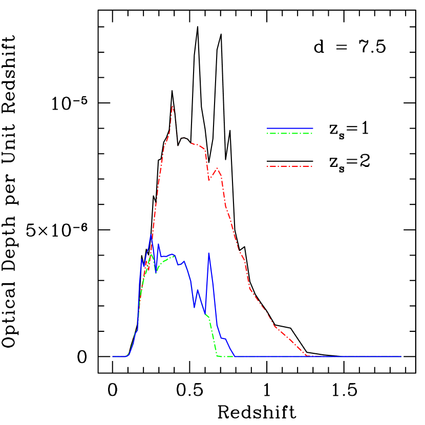
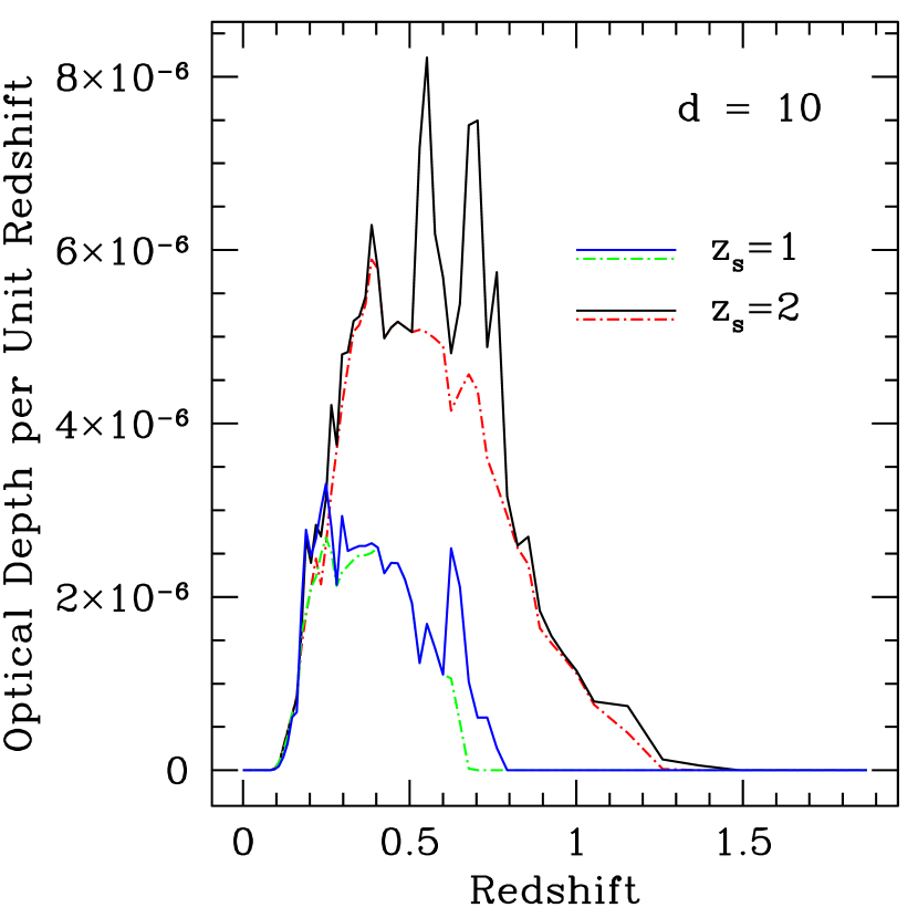
Figure 4: The evolution with redshift of the optical depth per unit redshift for gravitational arcs with length-to-width ratios equal to or larger than $d$. Solid lines include the effect of cluster mergers, while dashed lines do not. Upper curves refer to sources with $z_{\mathrm{s}}=2$ and lower curves to sources with $z_{\mathrm{s}}=1$.

The overall trend of the differential optical depth in Fig. 4 resembles individual cross sections, i.e. it drops to zero as the lenses approach the observer or the sources. The dashed (upper) curve for $z_{\mathrm{s}}=2$ broadly peaks at redshift $z_{p}\approx 0.4$, slightly larger than the typical redshift for the peak of the individual cross sections shown in Fig. 3. This is simply due to the fact that in the differential optical depth the lensing cross sections are weighted with the number density of structures within mass bins. It is interesting to note that the same peak occurs even in the corresponding solid curve, thus it is not due to dynamical processes in the cluster lenses, but rather to the combination of the mass evolution of the lenses with the particularly high lensing efficiency for clusters at that redshift.

Apart from that, the most remarkable result shown by the solid curves is that the impact of cluster mergers is important in particular at moderate and high redshifts, $0.5\lesssim z\lesssim 0.8$. The pronounced peaks in the differential optical depth seen there even after averaging over the halo sample indicate that cluster mergers can substantially increase the lensing optical depth of high-redshift clusters. Above redshift $0.5$, mergers almost double the optical depth.

Shifting the source plane from $z_{\mathrm{s}}=2$ to $z_{\mathrm{s}}=1$ significantly lowers the total optical depth as well as the impact of cluster mergers on the optical depth per unit redshift. The first effect is obviously due to the fact that for lower source redshift, the redshift interval of high lensing efficiency narrows. The second effect reflects that sources at lower redshift miss a significant part of the lensing haloes’ formation history and merger processes related with it.

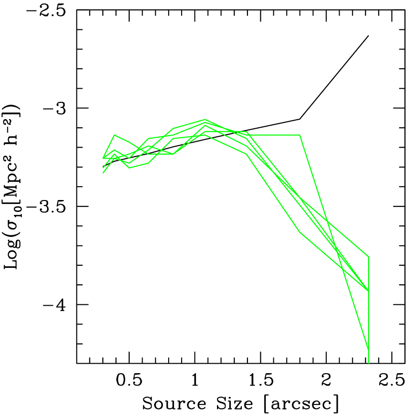
Figure 5: Cross section for gravitational arcs with length-to-width ratio exceeding $d=10$ for a dark-matter halo of $10^{15}\,M_{\odot}h^{-1}$ as a function of the source size in arc sec. Black and green lines show the results of the semi-analytic and of ray-tracing simulations, respectively, which are repeated with different random-number seeds for the ellipticities and the position angles of the sources, as in Fig. 1. The source redshift is $z_{\mathrm{s}}=1$, and the lens redshift is $z_{\mathrm{l}}=0.3$.

5.3 Sources Properties

A full analysis of the effect of various source properties on the cross sections of individual haloes is well beyond the scope of this paper. Moreover, the method we have outlined in the previous subsections is probably not the ideal tool for that purpose. For example, it would be of interest to check the variation of cross sections with the source size. Fig. 5 shows that numerical and semi-analytic cross sections agrees (as already shown) and initially increase with increasing source size. However, when the sources become too large compared to the size of the caustic structure, the assumption that the lensing properties are approximatively constant across the area of a source fails (see the Appendix for details). Thus, while numerical cross sections start to decrease because the sources are too large to be efficiently distorted, the semi-analytic cross section increases dramatically. We note that, as in the rest of this paper, dark matter haloes are modelled with NFW density profiles and elliptically distorted lensing potential.

Nonetheless, some testable effects can be briefly addressed here. The first is the influence of the shape (circular or elliptical) of the sources on the lensing efficiency. On this ground we can compare our results with Keeton (2001).

Figure 6: Cross section for gravitational arcs with length-to-width ratio exceeding $d=10$ for several haloes of increasing mass. Black and red lines refer to point-like or extended sources with area equal to that of a circle of radius $0.5^{\prime\prime}$, respectively. Short dashed lines indicate circular sources, long dashed lines refer to sources with random ellipticity drawn from the interval $[0,0.5]$ $\left(q_{s}\in[0.5,1]\right)$, and solid lines refer to sources with ellipticity $0.5$. Sources are at redshift $z_{\mathrm{s}}=1$ and the lens redshift is $z_{\mathrm{l}}=0.3$.

Fig. 6 shows the cross section of several dark-matter haloes of increasing mass as a function of the source ellipticity, as explained in the caption. We see in the Figure that the cross sections for small elliptical sources exceed those of small circular sources by a factor of $\approx 2$. This agrees with the findings of Keeton (2001). It is quite interesting to note that the corresponding increase is somewhat lower for larger sources. This is due to the fact that the cross section is on the average higher, thus the contribution from the source ellipticity is relatively less important.

Another quite important effect is the change of the cross section with the source redshift. Investigating this, we will keep the source size fixed at a radius of $0.5^{\prime\prime}$, since the angular diameter distance changes only a little over redshift 1.

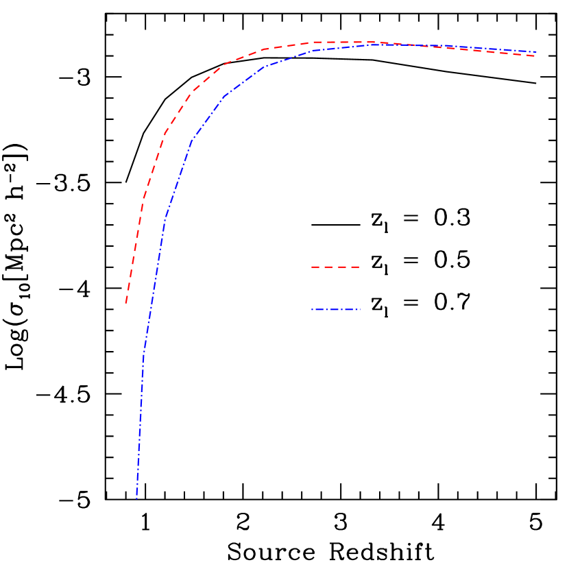
Figure 7: Cross section for arcs with length-to-width ratio exceeding $d=10$ for a dark matter halo of $10^{15}\,M_{\odot}h^{-1}$ as a function of the source redshift. Three different lens redshifts are considered, as labeled in the plot.

In Fig. 7 we plot the cross section for a single dark-matter halo of $10^{15}M_{\odot}h^{-1}$ as a function of the source redshift. We adopt three different lens redshifts, $0.3$, $0.5$ and $0.7$ respectively. The low-redshift end of that plot shows that the closer the lens is to the source, the lower the cross section is due to the geometrical suppression of the halo’s lensing efficiency (see the discussion in Sect. 5). The general trend is a rapid increase of the lensing cross section with increasing lens redshift followed by an almost constant phase and a slightly decreasing phase. This trend agrees with the general evolution of the lensing efficiency with the source redshift.

These few examples show how the influence of the source redshift and intrinsic properties on a cluster’s lensing efficiency is significant, in agreement with earlier work, and a deeper analysis of the consequences is certainly needed.

6 Summary and Discussion

We have described a novel method for semi-analytically calculating strong-lensing cross sections of galaxy clusters. The method first approximates the length-to-width ratio of images by the ratio of the eigenvalues of the Jacobian matrix of the lens mapping. The requirement that this ratio exceed a fixed threshold defines a stripe on both sides of the (tangential) caustic curve whose area approximates the cluster’s strong-lensing cross section.

This approach would be valid for infinitesimally small, circular sources. Extending it for elliptical sources is straightforward using the elegant technique developed by Keeton (2001). Extended sources can be taken into account after convolving the eigenvalue ratio with a suitable window function quantifying the source size. In order to speed up this convolution, we approximate it by a simple multiplication.

We have tested this method by detailed comparison with cross sections obtained from full ray-tracing simulations. We found excellent agreement within the (considerable) error bars of the ray-tracing results for a variety of lens masses and lens and source redshifts. Deviations occur for very weak lenses whose caustics are so small that the crucial assumption of the eigenvalue ratio’s not changing much across sources is no longer satisfied. In particular, our tests revealed that cross sections rapidly changing during merger events are well reproduced by our new method.

We then proceeded to apply the technique to a sample of halos whose history is described by simulated merger trees. The halos themselves are modelled as pseudo-elliptical halos with NFW density profile whose mass is given as a function of redshift by the merger tree. The merger trees are obtained from a sample of 46 cluster-sized halos numerically simulated in a cosmological volume. We followed the evolution of the halos by simulating merger events at times when the merger trees signal the accretion of a sub-halo with mass comparable to that of the main halo.

This technique allowed us to study the total optical depth for arc formation by the simulated cluster sample at a time resolution high enough for properly following merger events. Comparing the results to those obtained ignoring mergers, we found that the arc optical depth produced by clusters with moderated and high redshifts, $z\gtrsim 0.5$, is almost doubled by mergers.

The resuts just outlined may be potentially relevant in view of the high frenquency of arcs recently detected in clusters at moderate and high redshifts (Gladders et al., 2003; Zaritsky & Gonzalez, 2003). For example, Gladders et al. (2003) argue that some physical process must boost the lensing efficiency of high-redshift clusters which is likely connected with the dynamics and formation histories of the lensing clusters, as merger processes are. This conclusion was supported by (Horesh et al., 2005) after this paper was first submitted. Horesh et al. (2005) compare the lensing efficiency of matched observed and simulated (low-redshift) galaxy clusters with a realistic source population taken from the Hubble Deep Field. They find that real clusters are a little bit more efficient lenses than simulated ones, and though the difference is marginally significant, they argue it could be due to a selection effect connected with cluster mergers. In fact, cluster mergers increase not only the lensing efficiency, but also the $X$-ray luminosity (Randall et al., 2002), and the real clusters used by Horesh et al. (2005) are $X$-ray selected. In other words, the observed lensing clusters could be a biased sub-set of the entire cluster population.

The method described and developed here reduces computation times for strong-lensing cross sections by factors of $\sim 30$ compared to ray-tracing simulations. It thus becomes feasible to reliably compute strong-lensing probabilities describing an evolving cluster population by halos accreting mass as encoded by simulated merger trees, whose merging events can be studied at high time resolution. We shall apply this technique in forthcoming studies with special emphasis on the importance of cluster evolution for strong lensing.

Appendix A Approximate Convolution of a Function With a Step Function on the Source Plane

Consider an arbitrary function $\bar{R}(\@vec{y})$ defined on the source plane. Suppose we wish to convolve $\bar{R}(\@vec{y})$ with another function $g(\@vec{y})$, defined as in Eq. (14). The convolution is

$$h(\@vec{y})=(\bar{R}*g)(\@vec{y})=\int_{\mathbb{R}^{2}}\,\bar{R}(\@vec{z})\,g(\@vec{y}-\@vec{z})\mathrm{d}^{2}z\;.$$ (30)

Without loss of generality, any given point $\@vec{y}$ on the source plane can be chosen as the coordinate origin. This means that $y\equiv 0$, hence

$$h(0)=(\bar{R}*g)(0)=\int_{\mathbb{R}^{2}}\,\bar{R}(\@vec{z})\,g(\@vec{z})\mathrm{d}^{2}z\;.$$ (31)

Now, we choose a position $\@vec{u}$ on the lens plane such that $\@vec{z}=\@vec{z}(\@vec{u})$. Applying the lens mapping to the convolution above we obtain

$$h(0)=\int_{\mathbb{R}^{2}}\,R(\@vec{u})\,g(\@vec{u})\,\frac{\mathrm{d}^{2}u}{|\mu(\@vec{u})|}\;.$$ (32)

We assume that $\bar{R}(\@vec{y})$ does not vary much across a source. This assumption is satisfied in almost all interesting cases, except when the sources are at high redshift and the lens is close to them. In that case the critical curves are very small, thus the typical scale on which the lensing properties vary may be comparable with the angular extent of a source. However, even in that case the results of our method remain good, in particular in view of the substantial scatter in the ray-tracing results.

Within this assumption, we can expand the function $R(\@vec{x})$ into a Taylor series around zero, obtaining (summing over repeated indices)

$$h(0) \approx R(0)\int_{\mathbb{R}^{2}}\,g(\@vec{u})\,\frac{\mathrm{d}^{2}u}{|\mu(\@vec{u})|}+\frac{\partial R(0)}{\partial u_{i}}\int_{\mathbb{R}^{2}}u_{i}g(\@vec{u})\frac{\mathrm{d}^{2}u}{|\mu(\@vec{u})|}$$ (33)

$$+ \frac{1}{2}\frac{\partial^{2}R(0)}{\partial u_{i}\partial u_{j}}\int_{\mathbb{R}^{2}}u_{i}u_{j}g(\@vec{u})\frac{\mathrm{d}^{2}u}{|\mu(\@vec{u})|}\;.$$

The first integral is unity by normalisation, and the second vanishes because of the symmetry of $g(\@vec{x})$. Thus, Eq. (33) reduces to

$$h(\@vec{y}) \approx R(0)+\frac{1}{2}\frac{\partial^{2}R(0)}{\partial u_{i}\partial u_{j}}\int_{\mathbb{R}^{2}}u_{i}u_{j}g(\@vec{u})\frac{\mathrm{d}^{2}u}{|\mu(\@vec{u})|}$$ (34)

$$\equiv R(0)+\frac{1}{2}\frac{\partial^{2}R(0)}{\partial u_{i}\partial u_{j}}\Omega_{ij}\;.$$

Thus, we have to carry out the three integrals $\Omega_{11}$, $\Omega_{22}$ and $\Omega_{12}=\Omega_{21}$. We show the explicit calculation only for the first, as the others are quite similar:

$$\Omega_{11}\equiv\int_{\mathbb{R}^{2}}u_{1}^{2}g(\@vec{u})\frac{\mathrm{d}^{2}u}{|\mu(\@vec{u})|}=\frac{1}{\pi\zeta^{2}}\int_{D}u_{1}^{2}\frac{\mathrm{d}^{2}u}{|\mu(\@vec{u})|}\;,$$ (35)

where $D$ is the set of all positions $\@vec{x}$ on the lens plane where $\@vec{x}^{T}\Gamma\@vec{x}\leq 1$. The matrix $\Gamma$ defines the shape of the image formed from the source and can be written as $\Gamma=\mathcal{A}^{T}\mathcal{B}\mathcal{A}=\mathcal{A}^{T}\mathcal{A}/\zeta^{2}$. Obviously, the eigenvalues of $\Gamma$ are $\lambda_{\mathrm{t}}^{2}/\zeta^{2}$ and $\lambda_{\mathrm{r}}^{2}/\zeta^{2}$. We can now rotate into a reference frame in which $\mathcal{A}$ and thus also $\Gamma$ are diagonal. This is achieved by a rotating about an angle

$$\varphi=\frac{1}{2}\arctan\left(\frac{\gamma_{2}}{\gamma_{1}}\right)\;,$$ (36)

where $\gamma_{1}$ and $\gamma_{2}$ are the two shear components at the origin. This rotation is described by the orthogonal matrix

$$\mathcal{R}=\left(\begin{array}[]{cc}\cos\varphi&-\sin\varphi\\ \sin\varphi&\cos\varphi\\ \end{array}\right)\;.$$ (37)

With $\@vec{v}=R\@vec{u}$, this rotation, transforms Eq. (35) into

$$\Omega_{11} = \frac{1}{\pi\zeta^{2}}\int_{D}(v_{1}^{2}\cos^{2}\varphi+v_{2}^{2}\sin^{2}\varphi)\frac{\mathrm{d}^{2}v}{|\mu(\@vec{v})|}$$ (38)

$$+ \int_{D}(2v_{1}v_{2}\cos\varphi\sin\varphi)\frac{\mathrm{d}^{2}v}{|\mu(\@vec{v})|}$$

$$= \frac{\cos^{2}\varphi}{\pi\zeta^{2}}\int_{D}v_{1}^{2}\frac{\mathrm{d}^{2}v}{|\mu(\@vec{v})|}+\frac{\sin^{2}\varphi}{\pi\zeta^{2}}\int_{D}v_{2}^{2}\frac{\mathrm{d}^{2}v}{|\mu(\@vec{v})|}\;.$$

In the new coordinate system, $D$ is the set of all positions $\@vec{v}$ of the lens plane where

$$\frac{\lambda_{\mathrm{t}}^{2}}{\zeta^{2}}v_{1}^{2}+\frac{\lambda_{\mathrm{r}}^{2}}{\zeta^{2}}v_{2}^{2}\leq 1\;.$$ (39)

Now we can introduce polar elliptical coordinates $(\rho,\theta)$ by

$$v_{1}=\frac{\zeta}{|\lambda_{\mathrm{t}}|}\rho\cos\theta\;,\quad v_{2}=\frac{\zeta}{|\lambda_{\mathrm{r}}|}\rho\sin\theta\;,$$ (40)

in terms of which Eq. (38) becomes

$$\Omega_{11} = \frac{\zeta^{2}\cos^{2}\varphi}{\pi}\int_{0}^{2\pi}\int_{0}^{1}\rho^{3}\cos^{2}\theta\frac{\mathrm{d}\rho\mathrm{d}\theta}{\lambda_{\mathrm{t}}^{2}(\rho,\theta)}$$ (41)

$$+ \frac{\zeta^{2}\sin^{2}\varphi}{\pi}\int_{0}^{2\pi}\int_{0}^{1}\rho^{3}\sin^{2}\theta\frac{\mathrm{d}\rho\mathrm{d}\theta}{\lambda_{\mathrm{r}}^{2}(\rho,\theta)}\;.$$

As a second approximation, we shall assume that the tangential and radial eigenvalues do not vary much across a single image, so we can replace the eigenvalues by their mean values across the image. Then,

$$\Omega_{11} = \frac{\zeta^{2}\cos^{2}\varphi}{\pi\langle\lambda^{2}_{\mathrm{t}}\rangle}\int_{0}^{2\pi}\int_{0}^{1}\rho^{3}\cos^{2}\theta\mathrm{d}\rho\mathrm{d}\theta$$ (42)

$$+ \frac{\zeta^{2}\sin^{2}\varphi}{\pi\langle\lambda_{\mathrm{r}}^{2}\rangle}\int_{0}^{2\pi}\int_{0}^{1}\rho^{3}\sin^{2}\theta\mathrm{d}\rho\mathrm{d}\theta$$

$$= \frac{\zeta^{2}}{4}\left(\frac{\cos^{2}\varphi}{\langle\lambda_{\mathrm{t}}^{2}\rangle}+\frac{\sin^{2}\varphi}{\langle\lambda_{\mathrm{r}}^{2}\rangle}\right)\;.$$

Similarly, we find that

$$\Omega_{22}=\frac{\zeta^{2}}{4}\left(\frac{\cos^{2}\varphi}{\langle\lambda_{\mathrm{r}}^{2}\rangle}+\frac{\sin^{2}\varphi}{\langle\lambda_{\mathrm{t}}^{2}\rangle}\right)$$ (43)

and

$$\Omega_{12}=\frac{\zeta^{2}\sin\varphi\cos\varphi}{4}\left(\frac{1}{\langle\lambda_{\mathrm{r}}^{2}\rangle}-\frac{1}{\langle\lambda_{\mathrm{t}}^{2}\rangle}\right)$$ (44)

Substituting into Eq. (34), we obtain

$$h(0) \approx R(0)+\frac{1}{2}\frac{\partial^{2}R(0)}{\partial x_{1}^{2}}\left(\frac{\zeta^{2}\cos^{2}\varphi}{4\langle\lambda^{2}_{\mathrm{t}}\rangle}+\frac{\zeta^{2}\sin^{2}\varphi}{4\langle\lambda^{2}_{\mathrm{r}}\rangle}\right)$$ (45)

$$+ \frac{1}{2}\frac{\partial^{2}R(0)}{\partial x_{2}^{2}}\left(\frac{\zeta^{2}\cos^{2}\varphi}{4\langle\lambda^{2}_{\mathrm{r}}\rangle}+\frac{\zeta^{2}\sin^{2}\varphi}{4\langle\lambda^{2}_{\mathrm{t}}\rangle}\right)$$

$$+ \frac{\partial^{2}R(0)}{\partial x_{1}\partial x_{2}}\left(\frac{\zeta^{2}\cos\varphi\sin\varphi}{4\langle\lambda^{2}_{\mathrm{r}}\rangle}-\frac{\zeta^{2}\cos\varphi\sin\varphi}{4\langle\lambda^{2}_{\mathrm{t}}\rangle}\right)\;.$$

Within the framework of our approximations, we can thus replace the value of the function $R$ at a point of the lens plane with its convolution on the source plane at the corresponding point, represented by Eq. (45). In this way, we account for finite source sizes.

References

- Bartelmann (1996) Bartelmann, M. 1996, A&A, 313, 697
- Bartelmann et al. (1998) Bartelmann, M., Huss, A., Colberg, J., Jenkins, A., & Pearce, F. 1998, A&A, 330, 1
- Bartelmann et al. (1995) Bartelmann, M., Steinmetz, M., & Weiss, A. 1995, A&A, 297, 1
- Bartelmann & Weiss (1994) Bartelmann, M. & Weiss, A. 1994, A&A, 287, 1
- Bond et al. (1991) Bond, J., Cole, S., Efstathiou, G., & Kaiser, N. 1991, ApJ, 379, 440
- Cole & Lacey (1996) Cole, S. & Lacey, C. 1996, MNRAS, 281, 716
- Dalal et al. (2004) Dalal, N., Holder, G., & Hennawi, J. F. 2004, ApJ, 609, 50
- Eke et al. (1996) Eke, V., Cole, S., & Frenk, C. 1996, MNRAS, 282, 263
- Eke et al. (2001) Eke, V., Navarro, J., & Steinmetz, M. 2001, ApJ, 554, 114
- Gladders et al. (2003) Gladders, M., Hoekstra, H., Yee, H., Hall, P., & Barrientos, L. 2003, ApJ, 593, 48
- Golse & Kneib (2002) Golse, G. & Kneib, J.-P. 2002, A&A, 390, 821
- Hennawi et al. (2005) Hennawi, J., Dalal, N., Bode, P., & Ostriker, J. 2005, ArXiv Astrophysics e-prints; arXiv:astro-ph/0506171
- Hopkins et al. (2005) Hopkins, P., Bahcall, N., & Bode, P. 2005, ApJ, 618, 1
- Horesh et al. (2005) Horesh, A., Ofek, E., Maoz, D., et al. 2005, ApJ, accepted; preprint astro-ph/0507454
- Keeton (2001) Keeton, C. 2001, ApJ, 562, 160
- Lacey & Cole (1993) Lacey, C. & Cole, S. 1993, MNRAS, 262, 627
- Lacey & Cole (1994) Lacey, C. & Cole, S. 1994, MNRAS, 271, 676
- Lee et al. (2005) Lee, J., Kang, X., & Jing, Y. 2005, ApJ, 629, L5
- Li et al. (2005) Li, G., Mao, S., Jing, Y., et al. 2005, ArXiv Astrophysics e-prints; arXiv:astro-ph/0503172
- Meneghetti et al. (2003a) Meneghetti, M., Bartelmann, M., & Moscardini, L. 2003a, MNRAS, 346, 67
- Meneghetti et al. (2003b) Meneghetti, M., Bartelmann, M., & Moscardini, L. 2003b, MNRAS, 340, 105
- Meneghetti et al. (2000) Meneghetti, M., Bolzonella, M., Bartelmann, M., Moscardini, L., & Tormen, G. 2000, MNRAS, 314, 338
- Miralda-Escude (1993) Miralda-Escude, J. 1993, ApJ, 403, 497
- Navarro et al. (1995) Navarro, J., Frenk, C., & White, S. 1995, MNRAS, 275, 720
- Navarro et al. (1996) Navarro, J., Frenk, C., & White, S. 1996, ApJ, 462, 563
- Navarro et al. (1997) Navarro, J., Frenk, C., & White, S. 1997, ApJ, 490, 493
- Press & Schechter (1974) Press, W. & Schechter, P. 1974, ApJ, 187, 425
- Puchwein et al. (2005) Puchwein, E., Bartelmann, M., Dolag, K., & Meneghetti, M. 2005, A&A in press; preprint astro-ph/0504206
- Randall et al. (2002) Randall, S. W., Sarazin, C. L., & Ricker, P. M. 2002, ApJ, 577, 579
- Schneider et al. (1992) Schneider, P., Ehlers, J., & Falco, E. E. 1992, Gravitational Lenses (Springer Verlag, Heidelberg)
- Sheth & Tormen (1999) Sheth, R. & Tormen, G. 1999, MNRAS, 308, 119
- Sheth & Tormen (2002) Sheth, R. & Tormen, G. 2002, MNRAS, 329, 61
- Tormen et al. (2004) Tormen, G., Moscardini, L., & Yoshida, N. 2004, MNRAS, 350, 1397
- Torri et al. (2004) Torri, E., Meneghetti, M., Bartelmann, M., et al. 2004, MNRAS, 349, 476
- Wambsganss et al. (2004) Wambsganss, J., Bode, P., & Ostriker, J. 2004, ApJL, 606, 93
- White et al. (1993) White, S. D. M., Efstathiou, G., & Frenk, C. S. 1993, MNRAS, 262, 1023
- Zaritsky & Gonzalez (2003) Zaritsky, D. & Gonzalez, A. 2003, ApJ, 584, 691