VLT Diffraction Limited Imaging and Spectroscopy in the NIR: Weighing the black hole in Centaurus A with NACO

Abstract

We present high spatial resolution near-infrared spectra and images of the nucleus of Centaurus A (NGC 5128) obtained with NAOS-CONICA at the VLT. The adaptive optics corrected data have a spatial resolution of 0$\farcs$06 (FWHM) in K- and 0$\farcs$11 in H-band, four times higher than previous studies. The mean velocities and velocity dispersions of the ionized gas ([FeII]) are mapped along four slit positions. The [FeII] emission line width decreases from a central value of $\sigma\simeq 320$ km s^-1 to $\sigma\simeq 120$ km s^-1 at $\rm{r}\simeq 0\farcs 5$, and exceeds the mean rotation within this radial range. The observed gas motions suggest a kinematically hot disk which is orbiting a central object and is oriented nearly perpendicular to the nuclear jet. We model the central rotation and velocity dispersion curves of the [FeII] gas orbiting in the combined potential of the stellar mass and the (dominant) black hole. Our physically most plausible model, a dynamically hot and geometrically thin gas disk, yields a black hole mass of $\rm{M_{bh}=6.1^{+0.6}_{-0.8}\times 10^{7}M_{\sun}}$. As the physical state of the gas is not well understood, we also consider two limiting cases: first a cold disk model, which completely neglects the velocity dispersion, but is in line with many earlier gas disk models; it yields an $\rm{M_{bh}}$ estimate that is almost two times lower. The other extreme case is to model a spherical gas distribution in hydrostatic equilibrium through Jeans equation. Compared to the hot disk model the best-fit black hole mass increases by a factor of 1.5. This wide mass range spanned by the limiting cases shows how important the gas physics is even for high resolution data. Our overall best-fitting black hole mass is a factor of 2-4 lower than previous measurements. A substantially lower $\rm{M_{bh}}$ estimate when using higher resolution kinematics was also found for many other black hole mass measurements as HST data became available. With our revised $\rm{M_{bh}}$ estimate, Cen A’s offset from the $\rm{M_{bh}}$-$\sigma$ relation is significantly reduced; it falls above this relation by a factor of $\sim 2$, which is close to the intrinsic scatter of this relation.

1. INTRODUCTION

Galaxy merging, the formation of stellar spheroids, nuclear star-formation and the fueling of nuclear black holes appear to be all linked, forming a central theme in building galaxies. Most galaxies where these processes are currently acting, are so far away that the ‘sphere of influence’ of the black hole cannot be spatially resolved and that detailed studies of stellar populations are impossible. Yet, our own Galactic Center alone tells us that galaxy centers tend to become increasingly more interesting when observed at higher and higher spatial resolution (e.g. Schödel et al., 2002; Genzel et al., 2003). When zooming into the nucleus of Centaurus A (NGC 5128), recent HST imaging (NICMOS) and ISAAC observations have also revealed smaller and smaller ‘sub-systems’ (Schreier et al., 1998; Marconi et al., 2000, 2001). Cen A, the closest massive elliptical galaxy, the nearest recent merger, and one of the nearest galaxies with a significantly active nucleus provides a unique laboratory to probe the interconnection between these phenomena on scales that are contained in the central resolution element in any other object of its kind.
The intricate dust lane that hides the center of Cen A has not allowed optical high-resolution spectroscopy with HST. Infrared (IR) spectroscopy is thus increasingly important to open up the regime of dust shrouded nuclei and get accurate black hole mass measurements for these objects.
Cen A is especially interesting since the black hole mass deduced by Marconi et al. (2001) (M${}_{\rm{bh}}=2.0^{+3.0}_{-1.4}\times 10^{8}\rm{M}_{\odot}$) lies a factor of ten above the $\rm{M_{bh}}$-$\sigma$ relation (Ferrarese & Merritt, 2000; Gebhardt et al., 2000). This is the largest offset from the relation measured to date. It is important to check this value, since it can help us to understand the coevolution of black holes and their surrounding bulges in more detail.
We have initiated a program to study the central parsec of Cen A using NAOS/CONICA (Rousset et al., 1998; Lenzen et al., 1998) at the Very Large Telescope (VLT). The adaptive-optics assisted imager and spectrograph provides us with near infrared data from 1 to 5 $\mu$m at the diffraction limit of a 8m class telescope. The resolution is thus nearly fourfold that of HST in K-band.
The distance to Cen A is still under discussion. In a comprehensive review Israel (1998) gives a value of 3.40$\pm$0.15 Mpc. Tonry et al. (2001) finds a value of 4.2$\pm$0.3 Mpc from I-band surface brightness fluctuations, and recently, Rejkuba (2004) derived a distance of 3.84$\pm$0.35 Mpc from Mira period-luminosity relation and the luminosity of the tip of the red giant branch. Here, we assume a distance of D=3.5 Mpc to be consistent with the black hole mass measurements of Marconi et al. (2001) and Silge et al. (2005) that also used that value.
The paper is structured as follows: in Section 2 we present the observational strategy and the data reduction. Section 3 describes the treatment of the spectral data. Section 4 presents the dynamical modeling and the results for the black hole mass for Centaurus A, and Section 5 discusses the implications of these results.

2. OBSERVATIONS AND DATA REDUCTION

2.1. Adaptive Optics Observations

Near infrared observations were performed in 2004 March 28 and 31 with NAOS-CONICA (NACO) at the Yepun unit (UT4) of the very large telescope (VLT). NACO consists of the high-resolution near-infrared imager and spectrograph CONICA (Lenzen et al., 1998) and the Nasmyth Adaptive Optics System (NAOS) (Rousset et al., 1998). It provides adaptive-optics corrected observations in the range of 1-5 $\mu$m with 14$\arcsec$ to 54$\arcsec$ fields of view and 13 to 54 mas pixel scales.
The data were taken in visitor mode and seeing during observations was in the range 0$\farcs$3-0$\farcs$8 (as measured by the seeing monitor in V-band), with clear/photometric conditions.

Not seen in the visible, the active nucleus at the center of Centaurus A is an unresolved source in K-band of 10.9 mag as detected by Marconi et al. (2000). There are no potential reference stars bright enough ($m_{K}\leq$14 mag) for the wavefront correction at a distance of $\leq 30\arcsec$ to the nucleus, necessary for a good quality of correction at the nucleus. Therefore, we directly guided on the nucleus itself using the unique IR wavefront sensor implemented in NAOS. This strategy provides us the best possible wavefront correction in the vicinity of the active galactic nucleus (AGN). In fact we reach the diffraction limit of the VLT in K-band of FWHM $0\farcs 057$ and are not far off in H-band with $0\farcs 11$. During the observations the atmospheric conditions were stable and the performance of the IR wavefront sensor (WFS) was steadily very good. For observations in H-band we used the K-dichroic, i.e. all the nuclear K-band light for wavefront correction. While observing in K-band itself the only possibility to achieve a good performance of the WFS was to send 90% of the light to NAOS and only 10% to CONICA (i.e. use the N90C10 dichroic). This increases the exposure times by a factor of 10 and made it effectively impossible to go for spectroscopy in K-band.

2.2. K-Band Imaging

For the imaging we chose the strategy to jitter the field on five positions at a separation of 4$\arcsec$ and take a sky image at a dark position in the dust lane at a distance of $\sim$170$\arcsec$ South-East of the nucleus; this cycle was repeated 4 times. The on-chip exposure time was 120 s, yielding a total exposure time on the nucleus of 40 min. The resulting K-band image is shown in Figure 1.
The atmospheric conditions were stable and the seeing was $0\farcs 5$ at the start and $0\farcs 8$ at the end of the observations.

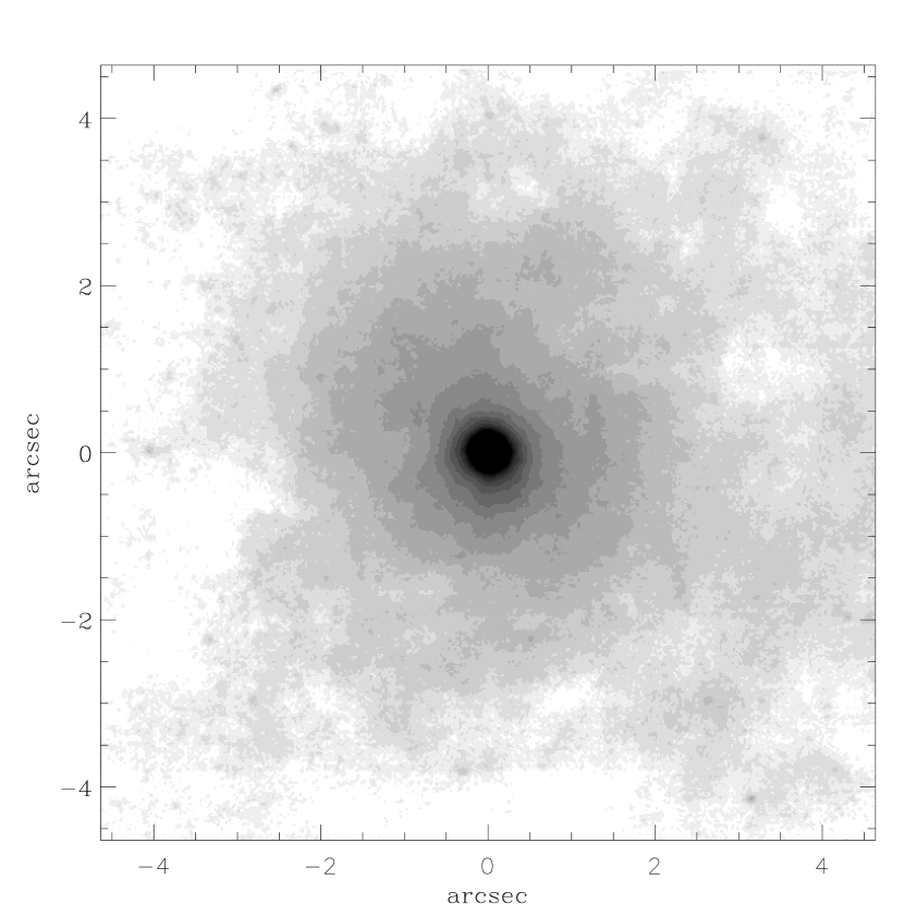
Figure 1.— K-band image taken with NACO. The nucleus is clearly visible as the unresolved source (FWHM=0$\farcs$06). North is up and East is to the left.

2.3. H-band spectroscopy

We took H-band spectra at 4 different position angles and chose three similar to Marconi et al. (2001) (P.A.= -44$\fdg$5, 32$\fdg$5, and 82$\fdg$5) in order to complement their findings with better spatial resolution. The fourth slit position (P.A.=70$\fdg$5) was chosen as to observe the nucleus and a foreground star simultaneously to monitor the point spread function (PSF) on a stellar reference. See Figure 2 for the positioning of the slits.
The observations were obtained with the $0\farcs 086$ slit and a grating with a wavelength range from $\lambda=1.37\mu$m to $1.84\mu$m. The pixel scale was $0\farcs 054$ leading to a slight under-sampling but shorter exposure times. The dispersion was 7.0 $\AA$ pixel^-1, yielding a resolution of R=1500 in H. At a given position angle, the observations went as follows: first, the loop for adaptive optics correction was closed. When a good performance of the WFS was reached, an acquisition image in H-band was taken. The slit was centered on the prominent nuclear peak with an accuracy of $\pm 0.2$pixel ($\pm 0\farcs 011$). The actual observations consisted of two sequences of exposures at 4 positions along the slit. This was done in order to perform sky subtraction and to avoid detector defects. The effective slit length is $14\arcsec$. The exposure time per frame was 300 s, leading to a total exposure time of 40 min per slit position angle.
Data reduction was performed using standard IRAF routines. The frames were first bias corrected and flat-fielded with spectroscopic lamp-flats. Then cosmic rays were rejected and the frames were wavelength calibrated and corrected for distortions using spectroscopic arc lamps.
To get the final 2-D spectrum the frames were aligned. This is done by shifting all frames to the same nuclear position. Finally, the frames were sorted by quality of wavefront correction, using both the width of the peak and the level of continuum flux.

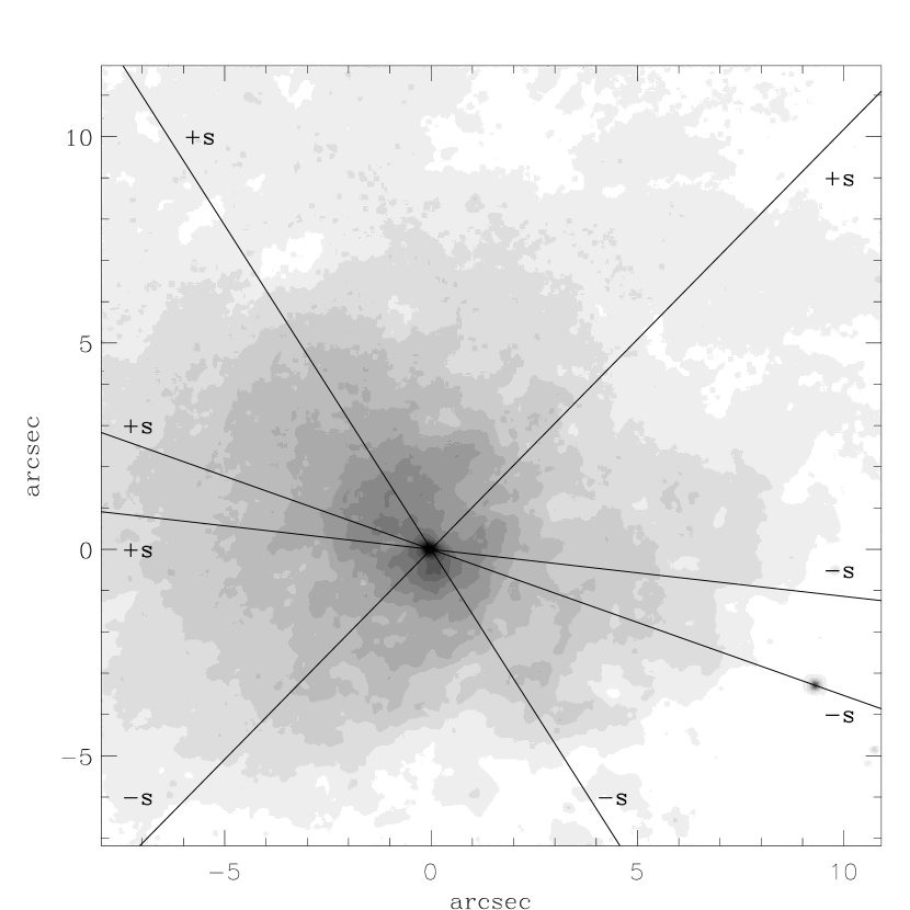
Figure 2.— Slit positions overlaid onto the H-band acquisition image. North is up and East is to the left. From North to South the slit positions are 32$\fdg$5, 70$\fdg$5, 82$\fdg$5, and -44$\fdg$5. The sign of the position along the slit used in the rotation curves is indicated by “+s” and “-s”. Note the foreground star that is in the slit at P.A.=70.5$\arcdeg$ in the lower right.

2.4. PSF-reconstruction

A difficult but crucial part of adaptive optics observations is the assessment of the point spread function (PSF). The PSF is highly dependent on the quality of the wavefront correction, quantified e.g. by the Strehl ratio. The Strehl ratio is set by the observable properties of the reference object (flux, size, contrast) but also by the atmospheric conditions (seeing, coherence time); it is therefore changing with time and needs to be monitored throughout the observations. In case of the K-band image a separate PSF reference star was observed directly after the nucleus with the same WFS setup. This star was chosen from the 2MASS point source catalogue (Cutri et al., 2003) to match Cen A’s nucleus as closely as possible: in angular proximity, magnitude and color.

Since the acquisition for NACO observations takes a non-negligible amount of time, going back and forth to the PSF star is a tedious and time-consuming task. On the other hand the measurement of a separate PSF-star at a given difference in time and position on the sky does not guarantee to give a good approximation on the actual on-source PSF. We therefore came to the conclusion that it is most suitable to measure the PSF in the science frame on the unresolved nucleus.

For emission line spectroscopy the strategy is to have the nucleus in the slit at all position angles and measure the PSF on this unresolved point-source for each frame. We tested this approach by choosing one position angle (P.A.$=70\arcdeg$) such that the nucleus plus a foreground star are simultaneously observed, and indeed, the widths of both light profiles are similar (compare Table 1).

We describe the normalized PSF empirically by a sum of two Gaussians; one narrow component describing the corrected/almost diffraction limited PSF core ($\sigma_{\rm{DL}}$) and one broader component which we later attribute to the seeing halo ($\sigma_{\rm{s}}$):

$$PSF(r)=\rm{\frac{F}{2\pi\sigma^{2}_{DL}}e^{-r^{2}/2\sigma^{2}_{DL}}+\frac{(1-F)}{2\pi\sigma^{2}_{s}}e^{-r^{2}/2\sigma^{2}_{s}},}$$

where F is the ratio of the flux of the narrow component and the total flux of the PSF (F = $\rm{flux_{DL}/flux_{total}}$). The quantity F provides a rough approximation of the Strehl ratio (S) which gives the quality of an optical system; S is defined as the observed peak flux divided by the theoretically expected peak flux of the Airy disk for the optical system (S = $\rm{peakflux_{DL}/peakflux_{Airy}}$). For the following analysis it is sufficient to measure the quantity F, which also gives an estimate of the quality of the adaptive optics correction.
The width of the fitted broad component can be compared with the seeing that is given in the header for each frame, as measured by the seeing monitor in V-band. One has to adjust the seeing estimates to the same wavelength, as the resolution $\theta$ depends on wavelength $\lambda$, as $\theta(\lambda)\sim\lambda^{-1/5}$. The individual components are given in Table 1 and are compared to the header information (adapted to H-band). The agreement between $\sigma_{\rm{s}}$ and $\sigma_{\rm{DIM}}$ is satisfactory in all cases. Notice also the good agreement between the width of the nucleus and the star at P.A.=70$\fdg$5. The adaptive optics correction is optimised for the position of the nucleus and is worse at the position of the star due to anisoplanetism.
Moreover it is obvious that the width of the narrow component depends on the seeing conditions.
Figure 4 shows the integrated flux over the two-component model PSF shown in Figure 3. Note that 50% of the flux lie within a radius of 0$\farcs$1 and 90% of the flux within 0$\farcs$3.
In the PSF model we did not account for the undersampling of the observed PSF, since the sampling problem is negligible compared to the general uncertainty in adaptive optics observations.

Table 1Reconstruction of the PSF

Object	P.A.	$\rm{FWHM_{DL}}$	$\rm{FWHM_{s}}$	$\rm{FWHM_{DIM(H)}}$	F
Nuc	32$\fdg$5	0$\farcs$11	0$\farcs$37	0$\farcs$37	0.23
Nuc	-44$\fdg$5	0$\farcs$15	0$\farcs$48	0$\farcs$48	0.18
Nuc	82$\fdg$5	0$\farcs$15	0$\farcs$53	0$\farcs$49	0.15
Nuc	70$\fdg$5	0$\farcs$11	0$\farcs$34	0$\farcs$35	0.22
Star	70$\fdg$5	0$\farcs$12	0$\farcs$36	0$\farcs$35	0.31

Figure 3.— Decomposition of the PSF for the slit position angle 82$\fdg$5. The data are over plotted by the 2-component PSF-model (solid line), where the dashed line indicates the corrected peak and the dotted line represents the uncorrected seeing halo. The bottom panel shows the residual between model and data.

Figure 4.— Integrated flux over the model PSF is shown for the slit position angle 82$\fdg$5 (to be compared with Figure 3).

3. RESULTS

3.1. Nuclear spectrum

A nuclear H-band spectrum centered on the continuum peak (Fig. 2) and extracted from a $0\farcs 054\times 0\farcs 086$ aperture is presented in Figure 5. The spectrum exhibits a power-law continuum with three [FeII] lines: $\lambda_{1}1.534\rm{\mu m}$, $\lambda_{2}1.644\rm{\mu m}$, and $\lambda_{3}1.677\rm{\mu m}$. We use the strongest line ($\lambda_{2}1.644\rm{\mu m}$) for our kinematical studies.

Figure 5.— Nuclear spectrum in H-band extracted from an aperture of $0\farcs 054\times 0\farcs 086$ at a slit position of 32$\fdg$5. The three [FeII] emission lines are indicated at the rest-frame wavelengths: $\lambda_{1}1.534\rm{\mu m}$, $\lambda_{2}1.644\rm{\mu m}$, and $\lambda_{3}1.677\rm{\mu m}$.

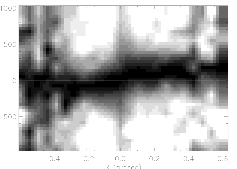
Figure 6.— Observed [FeII] $\lambda_{2}1.644\rm{\mu m}$ line on the NACO H-band spectrum at a slit position of -44$\fdg$5. To make the gas velocity curve more visible, each column of the spectrum was divided by the maximum value of the emission line in that column. The spectrum was then resampled on a 3 times finer grid by means of bilinear interpolation. The line indicates the systemic velocity of 532 km s^-1, which is shifted to zero for this plot.

Line-of-sight velocities, FWHMs, and surface brightnesses along each slit were obtained by fitting single Gaussians to the [FeII] emission line in each row of the continuum-subtracted two-dimensional spectra. The corresponding slit positions are shown in Figure 2 and listed in Table 1.

3.2. Gas Kinematics

We measure the gas kinematics on the ionised [FeII] line $\lambda 1.644\rm{\mu m}$ out to around $\pm 0\farcs 6$. Single Gaussians provide a good fit to the emission lines and are used to measure the position and width of the line. The fit is performed in IDL using a non-linear least squares fit to the line and the errors are the 1-$\sigma$ error estimates of the fit parameters. The center of the continuum peak is taken as a reference for the systemic velocity. We find a value of v_sys=532 km s^-1; in good agreement with the value v_sys=532$\pm$5km s^-1 measured by Marconi et al. (2001) from their gas kinematical data.
For the central 0$\farcs$3 only the four highest quality frames are considered in order to make use of the full resolution. The quality of the frames, i.e. their correction quality, is estimated on the basis of the width and the peak value of their continuum peak. Outside 0$\farcs$3, when the lineflux drops, all frames are taken into account and three pixels are binned to enhance the signal-to-noise ratio.
The rotation of the gas can be directly seen in Figure 6, where the line intensity was normalised by the peak intensity in each column. The rotation curves, velocity dispersion curves and emission-line surface brightness profiles are shown in Figure 7 for all slit positions.

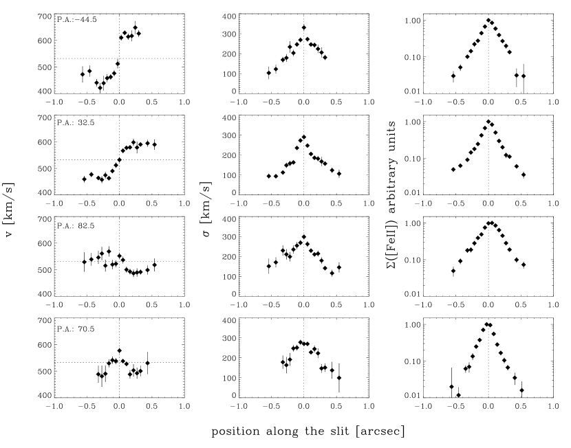
Figure 7.— Rotation curves (left panel), velocity dispersion profiles (middle panel) and emission line surface brightness profiles (right panel) along the 4 slit positions. For the position angles -44$\fdg$5 and 70$\fdg$5 some of the points shown in the surface brightness profile are missing for the v and $\sigma$ profiles.

The velocity dispersion is directly measured as the width of the lines. We corrected for instrumental broadening of 65 km s^-1, measured from the skylines.
The excellent spatial resolution of the NACO data is demonstrated in Figure 8 where we compare the NACO data points to the kinematical data published by Marconi et al. (2001) and Silge et al. (2005). The NACO velocity dispersions are often considerably smaller than the ISAAC velocity dispersions measured at the same location. The information given in Marconi et al. (2001) is not sufficient to find the reason for this discrepancy and we believe that our data points are correct.

Figure 8.— Comparison between the spatial resolution of the NACO data (filled diamonds), the ISAAC data (open triangles) (Marconi et al., 2001), and the GNIRS data (open squares) (Silge et al., 2005). The NACO and ISAAC data correspond to gas kinematics while the GNIRS data to stellar kinematics. In the left panel the rotational velocity is shown and in the right the velocity dispersion.

3.3. The Emission-Line Surface Brightness

The intrinsic surface brightness distribution of emission lines $\Sigma$ is an important ingredient in the model computations because it is the weight in the averaging of the observed quantities. It would be ideal to have an emission line image with higher spatial resolution than the spectra. Unfortunately, the resolution of the HST [FeII] narrow band image (Marconi et al., 2000) is not good enough to mimic the NACO data and therefore our approach is to match the emission-line fluxes as observed in the spectra. We extracted the emission line surface brightness from [FeII] directly from the spectra along the four slit positions (see Figure 7, right panels).
In order to get a parametrisation for the intrinsic surface brightness, we test different functional forms and convolve them with the PSF of the observations. The two-dimensional gas distribution is assumed to be a circular disk. We find that the intrinsic surface brightness of a disk is well fitted by a double exponential profile

$$\rm{I(r)=I_{0}e^{-r/r_{0}}+I_{1}e^{-r/r_{1}},}$$

where $\rm{r_{0}}$ and $\rm{r_{1}}$ are the scale radii, and $\rm{I_{0}}$ and $\rm{I_{1}}$ are the scale factors for the two components. This parametrisation was also used in Marconi et al. (2001). Since the observed emission line surface brightness along the slit at different position angles depends on the inclination of the circular gas disk (with respect to the observer) as well as on the PSF we fit the intrinsic emission-line fluxes for a median disk inclination of $45\arcdeg$ given the observational setup and conditions. The projected major axis of the [FeII] disk is at P.A.=$32\fdg 5$ (Marconi et al., 2000) and gets the highest weight in the fit, since the surface brightness along the major axis stays unchanged when the disk is inclined. The parameters that after PSF convolution best fit the surface brightness distribution along the different slit positions are I₁/I₀=0.018, r₀=0$\farcs$02, and r₁=0$\farcs$22. This parametrisation for the disk surface brightness is used in the dynamical models at all inclination angles. Compared to the fit values in Marconi et al. (2001) our scale radii are smaller due to higher spatial resolution. Given the shape of the [FeII] emission from the HST narrowband image (Marconi et al., 2000), the axis ratio of a possible gas disk is $\sim$1:2 which corresponds to an inclination angle of 60$\arcdeg$, given a circular disk structure. However, as found before by Marconi et al. (2001) there is a mismatch between the photometric major axis of the [FeII] gas disk and its kinematical major axis (line-of-nodes), which they find to lie between $-10\arcdeg>\zeta>-14\arcdeg$.

4. DYNAMICAL MODEL

In this section we outline the models describing the motions of the ionised gas in the combined gravitational potential of the (putative) central black hole and the stars. This modeling also requires a careful discussion of the gas geometry, as well as the physical state of the ionised gas, whose measured velocity dispersion far exceeds the expected thermal broadening.

4.1. The Stellar Mass Model

The first step in the dynamical modeling is to estimate the stellar contribution to the central potential from the stellar surface density. For the deprojection of the observed surface brightness distribution into the stellar luminosity density we applied the Multi-Gaussian expansion (MGE) method (Monnet, Bacon, & Emsellem, 1992; Emsellem, Monnet, & Bacon, 1994). Specifically, we obtained an MGE fit to a composite set of 2-dimensional K-band images using the method and software of Cappellari (2002). The MGE fit was performed using the NACO K-band image ($0^{\prime\prime}<r<7^{\prime\prime}$), the NICMOS F222M image (Schreier et al., 1998) ($2^{\prime\prime}<r<16^{\prime\prime}$), and the 2MASS Large galaxy atlas (LGA) K-band image (Jarrett et al., 2003) for larger radii ($8^{\prime\prime}<r<365^{\prime\prime}$).
The sky-subtraction was performed relative to the 2MASS LGA image, which is taken to be the sky-clean reference. The flux calibration of the NACO and NICMOS data is also referenced to the 2MASS image.

To get a parametrisation of the NACO K-band PSF we fit a full MGE model to the composite image of NGC 5128 (without giving the code a prior PSF estimate). We then selected the central four Gaussian components, that clearly described the unresolved nucleus, as the PSF. Its parametrisation is $\rm{PSF(R)=\sum_{i=1}^{N}G_{i}\,exp[-R^{2}/(2\sigma_{i}^{*2})]/(2\pi\sigma_{i}^{*2})}$, and the numerical values of the relative weights $G_{i}$ (normalised such that $\sum_{i=1}^{N}G_{i}=1$) and of the dispersions $\sigma_{i}^{*}$ are given in Table 2. This PSF was then fixed in the MGE fit to the composite image, where we neglected PSF convolution of the NICMOS and 2MASS images since these are only used at radii $r>2^{\prime\prime}$ and the NACO image has a much higher resolution.

Table 2MGE PSF parametrisation

i	$G_{i}$	$\sigma_{i}^{*}$	FWHM${}_{i}^{*}$
1…..	0.0004	0$\farcs$005	0$\farcs$012
2…..	0.1590	0$\farcs$031	0$\farcs$074
3…..	0.3034	0$\farcs$062	0$\farcs$145
4…..	0.5372	0$\farcs$143	0$\farcs$336

Figure 9 shows a comparison between the observed photometry and the MGE model along four different position angles in the galaxy, while Table 3 gives the corresponding numerical values of the analytically deconvolved MGE parametrisation of the galaxy surface brightness

$$\Sigma(x^{\prime},y^{\prime})=\sum_{i=1}^{N}\frac{L_{i}}{2\pi\sigma_{i}^{2}q^{\prime}_{i}}\exp\left[-\frac{1}{2\sigma_{i}^{2}}\left(x^{\prime 2}+\frac{y^{\prime 2}}{q^{\prime 2}_{i}}\right)\right],$$

where $(x^{{}^{\prime}},y^{{}^{\prime}})$ are the coordinates on the plane of the sky and N is the number of the adopted Gaussian components, having total luminosity $L_{i}$ , dispersion $\sigma_{i}$, and observed axial ratio 0.8$\leq q_{i}^{{}^{\prime}}\leq$1.0. In Table 3 the central unresolved component (which we attribute to the AGN) is removed. We only account for the stellar light distribution in the Multi-Gaussian expansion model.

Table 3MGE parametrisation of the deconvolved K-band surface brightness of Cen A

i	Li [$\times 10^{9}L_{\odot,K}$]		$\sigma_{i}$		q${}^{{}^{\prime}}_{i}$
1…..	0.	113	0$\farcs$	45	0.	882
2…..	0.	297	1$\farcs$	48	0.	812
3…..	1.	13	3$\farcs$	27	1.	000
4…..	1.	25	6$\farcs$	68	1.	000
5…..	5.	07	14$\farcs$	3	0.	879
6…..	15.	5	38$\farcs$	0	1.	000
7…..	19.	6	78$\farcs$	6	1.	000
8…..	23.	7	130$\farcs$	9	0.	807
9…..	5.	24	365$\farcs$	8	0.	800

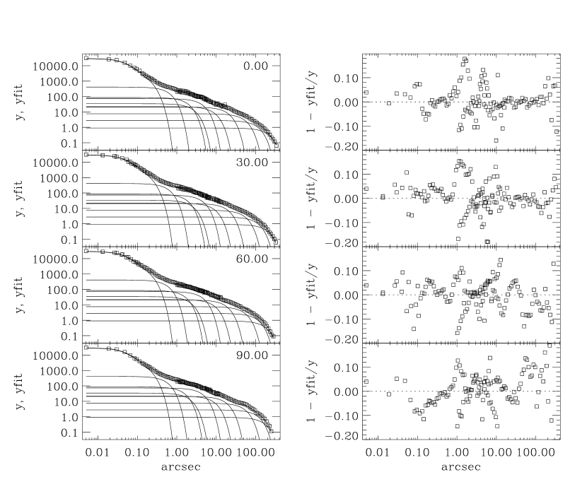
Figure 9.— Comparison between the NACO $(0^{\prime\prime}<R<7^{\prime\prime})$, NICMOS $(2^{\prime\prime}<R<16^{\prime\prime})$, and 2MASS LGA $(8^{\prime\prime}<R<365^{\prime\prime})$ K-band surface brightness (open squares) of Centaurus A and the corresponding best-fit MGE model (solid line) as a function of radius R. On the left the MGE fit is shown for inclination angles between $0\arcdeg$ and $90\arcdeg$, while the right panels show the corresponding residuals.

Using this radial profile of K-band (volume) emissivity, we fix the stellar mass-to-light ratio by constructing an isotropic spherical Jeans model and matching it over the radial range $3^{\prime\prime}<r<10^{\prime\prime}$ to the stellar kinematics ($\sqrt{v_{*}^{2}+\sigma_{*}^{2}}$) published recently by Silge et al. (2005). The innermost $3^{\prime\prime}$ are excluded from the fit to minimise the influence of the black hole. We find a best-fitting central mass-to-light ratio $\rm{M/L_{K}=(0.72\pm 0.04)}$ $\rm{M_{\odot}/L_{\odot}}$ in agreement with the best-fitting model of Silge et al. (2005). This agreement of the mass-to-light ratio from Schwarzschild and Jeans modeling is supported by the recent work of Cappellari et al. (2006).

4.2. Geometry and Kinematics of the [FeII] gas

The central [FeII] velocity curves (Figure 7) suggest that we see gas rotating in a flattened geometry around a central mass concentration, presumably dominated by a black hole. The velocity dispersion in the very center is quite high ($\sim$300 km s^-1 in the central pixel), well in excess of the mean rotation seen. In part this high dispersion may be attributed to rapid but spatially unresolved rotation.
As the underlying physical origin of the observed high gas dispersion is not clear a priori, we consider at least three geometric models:

1. the gas lies in a geometrically thin, kinematically cold disk and is in Keplerian motion around the black hole,
   

2. the gas forms a geometrically thin, kinematically hot disk that is in radial hydrostatic equilibrium,
   

3. the gas lies in a spherical distribution of collisionless cloudlets and can be modeled through Jeans equation.
   

Note that cases 1. and 3. are extreme physical assumptions and we consider them as limiting cases. In all three cases the gas is moving in the combined potential of the surrounding stars and of the central black hole; the self gravity of the gas is negligible (given the estimated mass of the ionised gas is $\sim 10^{3}M_{\odot}$ (Marconi et al., 2001) and the mass of the innermost Gaussian representing the stars is already $\sim 8\times 10^{7}M_{\odot}$ (see Table 3)). The underlying stellar mass distribution is the same in all models, with M/L fixed by the stellar kinematics at larger radii (see previous section).
The mismatch between the kinematical and photometric major axis of the gas disk, found before by Marconi et al. (2001) introduces a degeneracy between the inclination angle ($i$) of the gas disk and the position of its line-of-nodes ($\zeta$). We fear that our long-slit data will not be sufficient to constrain both $i$ and $\zeta$. We therefore make use of the inclination angle of the radio jet which sets the lower limit of the disk inclination in the standard picture of an orthogonal disk-jet geometry. Tingay et al. (1998) derived a value of $50\arcdeg<i<80\arcdeg$. Given this prior information, we set up our thin disk models.

4.3. Model 1: Thin cold disk model

We follow the widely used approach (e.g. Macchetto et al., 1997) which assumes the gas to lie in a thin disk around the black hole, moving on circular orbits; its observed velocity dispersion is assumed to be solely due to rotation. We constructed a model using the IDL software developed in Cappellari et al. (2002). This modeling can deal with multiple component PSFs, different PSFs for different data-subsets, and a general gas surface brightness distribution. Pixel binning and slit effects are taken into account to generate a two-dimensional model spectrum with the same pixel scale as the observations. Like in the data analysis, the rotational velocity and velocity dispersion is determined by fitting simple Gaussians to each row of the model spectrum. We make no velocity offset correction (van der Marel et al., 1997; Maciejewski & Binney, 2001; Barth et al., 2001), since the slit width ($0\farcs 086$) is comparable to the FWHM of the PSF.
The predicted velocity and velocity dispersion profiles of this model depend on the intrinsic surface brightness distribution of the emission lines, the PSF, plus the following parameters:

1. the inclination, $i$, of the gas disk ($i=0\arcdeg$ is face-on, 90$\arcdeg$ edge-on)
   

2. the angle between the projected major axis of the disk (line of nodes), $\zeta$, and the slit positions
   

3. the black hole mass, M_bh; the stellar mass profile is fixed.
   

We describe the “intrinsic velocity dispersion” of the gas in the model by a double exponential parametrisation of the form

$$\sigma_{R}=\sigma_{0}e^{-r/r_{0}}(1+\epsilon e^{-r/r_{1}}),$$

without using it in the dynamics. The parameters $\sigma_{0}$, $\epsilon$, $r_{0}$, and $r_{1}$ are fixed through comparison of the observed dispersion profile to a flux-weighted convolution of the intrinsic velocity dispersion profile with the PSF and the size of the aperture. The parameters that give a good fit to the velocity dispersion at all slit positions in the cold disk model are, $\sigma_{0}$=140 km s^-1 , $\epsilon\simeq 0.25$, $r_{0}=0\farcs 9$, and $r_{1}=0\farcs 2$. We do not know the source for this high velocity dispersion and simply ignore it in the kinematically cold disk model. To reduce the number of free parameters in the model we evaluate the rotation curves for three fixed inclinations ($45\arcdeg$, $60\arcdeg$, and $70\arcdeg$) and fixed the intrinsic surface brightness density of the gas disk beforehand (cf. Section 3.3).
In Table 4 we give the best-fitting black hole masses for each inclination angle individually; we also give the resulting $\chi^{2}$ values to get the overall best-fitting model. The $1\sigma$, $2\sigma$, and $3\sigma$ contours are shown in Figure 10 for the two degrees of freedom, black hole mass and line-of-nodes. The three sets of contours correspond to the relevant inclination angles of the gas disk (i=$45\arcdeg$,$60\arcdeg$, and $70\arcdeg$) where the best-fitting inclination angle, i=$45\arcdeg$, is indicated by a solid line.

Table 4Best Fit Values - Cold Disk Model

i	Mbh [$M_{\odot}$]	$\zeta$	$\chi^{2}_{\rm{tot}}$
45$\arcdeg$	$(4.0\pm 0.2)\times 10^{7}$	$-27\arcdeg\pm 4\arcdeg$	46.1
60$\arcdeg$	$(3.2\pm 0.2)\times 10^{7}$	$-28\arcdeg\pm 4\arcdeg$	47.1
70$\arcdeg$	$(3.2\pm 0.1)\times 10^{7}$	$-36\arcdeg\pm 2\arcdeg$	47.1

Figure 10.— Fitting a cold gas disk: the $\chi^{2}$ contours are shown for the two parameter fit of black hole mass vs. projected major axis $\zeta$ for the three inclination angles. The best cold model is at an inclination angle of $45\arcdeg$ and the corresponding contours are plotted in solid lines. The best-fitting values are $\zeta=-27\arcdeg\pm 4\arcdeg$ and M${}_{\rm{bh}}=(4.0\pm 0.2)\times 10^{7}M_{\odot}$. The three contours give the formal 68.3%, 95.4%, and 99.73% (thick) confidence levels.

The overall best-fitting cold gas model is obtained at an inclination angle of $45\arcdeg$. Figure 11 shows the observational data in comparison to the model. The parametrisation of the surface brightness, shown in the third row, is fixed beforehand and not included in the fit here (compare Section 3.3). The parameters that lead to this fit are $\zeta=-27\arcdeg$ and M${}_{\rm{bh}}=4.0\times 10^{7}M_{\odot}$.
However, the minimum $\chi^{2}$ values are comparable for all three cases, i.e. their differences are smaller than the 1$\sigma$ level, and we therefore cannot constrain the inclination angle of the gas disk with our long-slit data. We conclude that the black hole mass for a dynamically cold, geometrically thin disk model is M${}_{\rm{bh}}=(4.0^{+0.2}_{-1.0})\times 10^{7}M_{\odot}$.

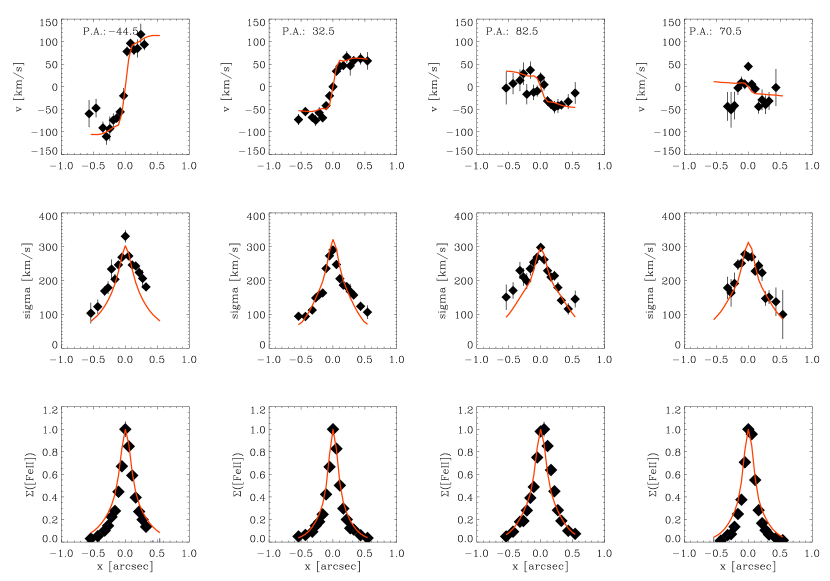
Figure 11.— The observational data is shown in comparison to the best fitting cold disk model at 45$\arcdeg$ inclination angle. The best-fitting parameters are $\zeta=-27\arcdeg$ and M${}_{\rm{bh}}=4.0\times 10^{7}M_{\odot}$. The velocity dispersion as well as the surface brightness are parametrised by a double exponential function which were fixed beforehand and not fitted here.

4.4. Model 2: Thin hot disk model

This model is identical to the previous one except that we now interpret the “intrinsic velocity dispersion” as a gas pressure component. As mentioned above, we do not know the physical origin of this high velocity dispersion of the gas, nevertheless, we include it in the dynamical analysis.
Any pressure support will require less rotation for dynamical equilibrium at a given black hole mass. In other words, the black hole mass needs to be larger to cause the same mean rotational velocity. The classic approach to account for velocity dispersion is to apply an asymmetric drift correction (e.g Barth et al. (2001)), but the approximate equations are only applicable if $\sigma/v$ is small. However, in the case of Cen A, $\sigma/v$ even exceeds unity and we therefore chose another approach: we assume the gas disk to be geometrically flat but with an isotropic pressure; on this basis we construct an axisymmetric Jeans model in hydrostatic equilibrium to model the observations.
We assume that the [FeII] surface brightness of the gas disk $\Sigma_{g}(x,y)$ reflects the tracer gas density $\rho_{g}(x,y)$, and that the gas moves in the joint potential $\Phi$ of the stars and the central black hole. The Jeans equation for this situation reads (Binney & Tremaine, 1987, Eq.4-64a):

$$\frac{R}{\rho_{g}}\frac{\partial(\rho_{g}\sigma_{R}^{2})}{\partial R}+R\frac{\partial\Phi}{\partial R}=\overline{v_{\Phi}}^{2},$$

where R is the projected radius, and $\sigma_{R}$ and $\overline{v_{\Phi}}$ are the radial velocity dispersion and the azimuthal velocity of the gas, respectively, and both are functions of R.
We again parametrise the gas dispersion profile by a double exponential function of the form:

$$\sigma_{R}=\sigma_{0}e^{-r/r_{0}}(1+\epsilon e^{-r/r_{1}}),$$

and we fit for the best set of parameters ($\sigma_{0}$=140 km s^-1, $\epsilon\simeq 0.25$, $r_{0}=0\farcs 9$, and $r_{1}=0\farcs 2$) to get the intrinsic dispersion profile.
The assumption that the gas disk is infinitesimally thin does most probably not reflect the real physical properties but was chosen to eliminate line-of-sight integrations through a 3-dimensional gas distribution.
Table 5 summarises the best fit parameters and the corresponding $\chi^{2}$ values for the different inclination angles of the “hot” gas disk model. The $1\sigma$, $2\sigma$, and $3\sigma$ contours are plotted in Figure 13.

Table 5Best Fit Values - Hot Disk Model

i	Mbh [$M_{\odot}$]	$\zeta$	$\chi^{2}_{\rm{tot}}$
45$\arcdeg$	$(6.1\pm 0.3)\times 10^{7}$	$-27\arcdeg\pm 3\arcdeg$	52.1
60$\arcdeg$	$(5.6\pm 0.3)\times 10^{7}$	$-25\arcdeg\pm 2\arcdeg$	54.0
70$\arcdeg$	$(6.4\pm 0.3)\times 10^{7}$	$-25\arcdeg\pm 2\arcdeg$	53.7

The best-fitting hot disk model favors a black hole mass of M${}_{\rm{bh}}=(6.1\pm 0.3)\times 10^{7}M_{\odot}$ and $\zeta=-27\arcdeg\pm 3\arcdeg$, at an inclination angle of $45\arcdeg$. It is shown in Figure 12 for comparison. The increased total $\chi^{2}$ value (compared to the cold disk model) can be explained by the reduced number of degrees of freedom, since in the hot disk model the velocity dispersion and the rotational velocity are coupled through Jeans equation. However, the difference between the two fits is small ($<2\sigma$ confidence level) and the large velocity dispersion lead us to consider this model a better description of the physical properties at the center of Centaurus A.

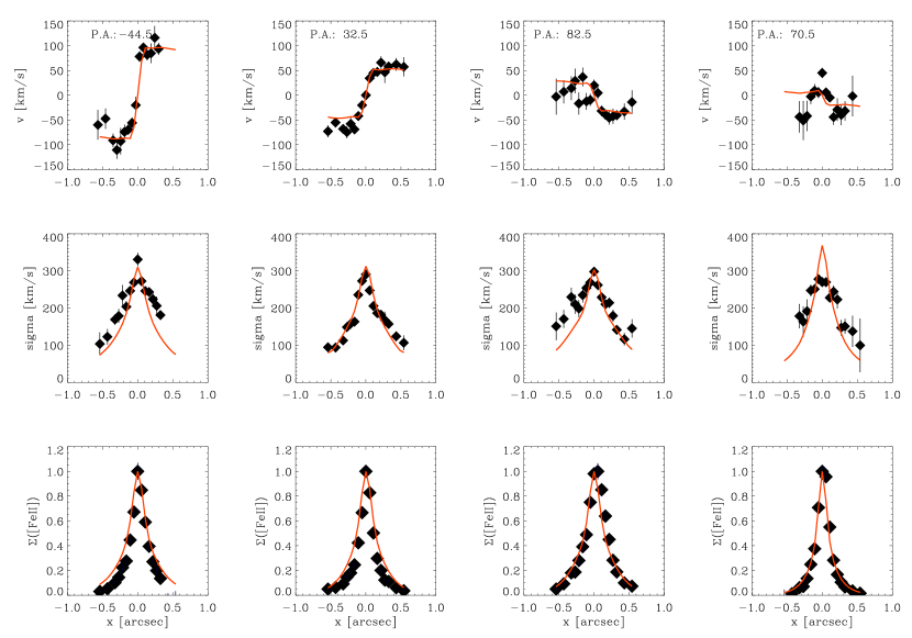
Figure 12.— The best-fitting hot disk model with parameters $\zeta=-27\arcdeg$ and M${}_{\rm{bh}}=6.1\times 10^{7}M_{\odot}$. In this model, $v$ and $\sigma$ are interwined through Jeans equation. Note that despite the higher black hole mass (compared to the cold disk model), the model curves drop beyond $0\farcs 3$ and match the observed data better. The model of the surface brightness is fixed beforehand and not fitted here.

Figure 13.— Fitting the ’hot’ gas disk: the $\chi^{2}$ contours are shown for the two parameter fit of black hole mass vs. projected major axis $\zeta$ for the three inclination angles. The best hot model is at an inclination angle of $45\arcdeg$ and the corresponding contours are plotted in solid lines. The best fitting values are $\zeta=-27\arcdeg\pm 3\arcdeg$ and M${}_{\rm{bh}}=(6.1\pm 0.3)\times 10^{7}M_{\odot}$. The three contours give the formal 68.3%, 95.4%, and 99.73% (thick) confidence levels.

4.5. Model 3: Spherical Jeans model

In this final modeling approach, we account for the fact that the high gas velocity dispersion is not consistent with the assumption of a thin disk. Alternatively, we assume the gas spherically symmetric distributed in individual clouds that move ballistically (i.e. t_coll$>>$t_dyn). Given the observational facts (rotation curves along certain slit positions, gas disk observed by Marconi et al. (2000)), this model is not very likely to describe the physical properties of the central region in Cen A. However, it gives an upper limit on the black hole mass, compared with disk models at non-extreme inclinations, and is implemented fairly easily. We construct a spherical Jeans model where we assume the following:

1. the gas density is given by its emissivity
   

2. the gas cloud distribution is spherical
   

3. the gas clouds move in the potential given by the stars and the possible central black hole
   

4. the stellar mass-to-light-ratio is constant throughout the relevant range ($<2^{\prime\prime}$)
   

5. the stars are in spherical symmetry.
   

Here, we construct a model with a Multi-Gaussian-expansion both for the stellar photometry and for the gas distribution. The gas surface brightness is given by the HST [FeII] narrow band image (Marconi et al., 2000) and fitted by an MGE model.
Following Tremaine et al. (1994) in the spherical case the solution of Jeans equation for the projected rms velocity reduces to

$$(v^{2}+\sigma^{2})_{p}(R)=\frac{2G}{\Upsilon\Sigma_{g}(R)}\int_{R}^{\infty}\frac{\rho_{g}(r)M_{tot}(r)}{r^{2}}(r^{2}-R^{2})^{1/2}dr,$$

where $\Upsilon$ is the stellar mass-to-light ratio, $\Sigma_{g}(R)$ is the surface brightness of the gas, $\rho_{g}(r)$ is the density of the gas and $M_{tot}(r)$ is the mass of the stellar body and the central dark object.
Again, the stellar mass-to-light ratio is fixed at a value of $\Upsilon=0.72\rm{M}_{\odot}/\rm{L}_{\odot}$, that we derived in section 4.1. The best fitting black hole mass that we find with the spherical Jeans model is $(1.0\pm 0.5)\times 10^{8}M_{\odot}$. The comparison between the measured and the modelled rms velocity ($\sqrt{v^{2}+\sigma^{2}}$) is shown in Figure 14.

Figure 14.— Comparison between the measured rms velocity (filled diamonds) and the spherical Jeans model (open diamonds) for the gas. The best fitting black hole mass is M${}_{\rm{bh}}=(1.0\pm 0.5)\times 10^{8}M_{\odot}$.

5. DISCUSSION

The availability of adaptive optics instrumentation opens up new realms of ground based observations. Drawing on kinematic data with unprecedented spatial resolution we present a dynamical model of the black hole in the nucleus of Centaurus A. The spatial resolution that we reach in our H-band spectra is $0\farcs 11$ (= 1.8 pc at a distance of 3.5 Mpc) that is a factor of 3 to 4 higher than from the previous ground based observations with ISAAC by Marconi et al. (2001). At large radii ($>0\farcs 3$) our data are in agreement with their gas kinematical data, but our high resolution data reveals the steep gradient of the rotation curve in much more detail (see e.g. Figure 7). The rotation curves show a smooth behavior and the slit position that shows the fastest rotation (P.A.=$-44\fdg 5$) is nearly perpendicular to the jet direction (P.A.$\sim 51\arcdeg$). This suggests the picture of gas orbiting in a flattened geometry (presumably a disk) around the central black hole, with the jet pointed along the disk angular momentum vector.

5.1. Black hole mass

In this paper we present three different dynamical modeling approaches to describe the gas kinematics in the central $\sim 2^{\prime\prime}\simeq$ 33pc of NGC5128. Two of the models are clearly conceptually inconsistent with the data, either neglecting the dominant velocity dispersion of the gas (Model 1; cold disk), or the disk-like geometry of the velocity field (Model 3; isotropic, spherical Jeans). We have laid out these extreme models as limiting cases, which would result in a broad mass range, $2.7\times 10^{7}M_{\odot}$ $<$ M_bh $<$ $1.5\times 10^{8}M_{\odot}$, and to demonstrate how important the gas physics is, even in light of high resolution data. Our physically most plausible model is a hot disk model at an inclination angle of $45\arcdeg$; the corresponding black hole mass is M${}_{\rm{bh}}=6.1^{+0.6}_{-0.8}\times 10^{7}M_{\odot}$ with a line-of-nodes at $\zeta=-27\arcdeg\pm 4\arcdeg$. We consider this model the best-fitting since it accounts for the high velocity dispersion of the gas combined with a disk-like gas structure, as suggested by the smooth rotation curves. The assumption of a geometrically thin disk is not physically motivated but was chosen to eliminate line-of-sight integrations through an underconstrained 3-dimensional gas distribution.

Our disk model meshes well with other constraints on the central geometry of NGC 5128: e.g. Tingay et al. (1998) derived a jet position angle of $\sim 51\arcdeg$. If we assume that the accretion disk and surrounding gas disk is at right angles, we would expect its line-of-nodes to be at $\sim-39\arcdeg$. Moreover, from the direction of the jet and counter-jet they derived a value for the jet inclination of $50\arcdeg<i<80\arcdeg$ with respect to the line-of-sight. Our best-fitting inclination angle of $45\arcdeg$ is close to their lower value, but our long-slit data do not tightly constrain the inclination angle. This was also the main source of uncertainty for the black hole mass in the previous study by Marconi et al. (2001). If we were to consider a gas disk inclination to be as face-on as 25$\arcdeg$ (inconsistent with the jet inclination), the black hole mass would increase to $\sim 1.2\times 10^{8}M_{\odot}$ in the hot disk case.

The unsettled question of inclination will presumably be solved with the analysis of integral field spectroscopy data taken with SINFONI at the VLT. The full 2-D velocity field data provide an excellent means of modelling black hole masses from gas as well as stellar kinematics.

Our best-fit value for the line-of-nodes is only $\sim 12\arcdeg$ away from the “expected” value of $\sim-39\arcdeg$, much closer than the value derived by Marconi et al. (2001), $-10\arcdeg>\zeta>-14\arcdeg$. Nonetheless, this confirms that the kinematical line-of-nodes does not coincide with the projected major axis of the gas disk (P.A.$\simeq 33\arcdeg$) seen in Pa$\alpha$ and [FeII] with NICMOS (Schreier et al., 1998; Marconi et al., 2000).
The value that we derived for the black hole mass from the best-fitting hot disk model ($6.1^{+0.6}_{-0.8}\times 10^{7}M_{\odot}$) is significantly lower than the values both from stellar kinematics presented by Silge et al. (2005) (M${}_{\rm{bh}}=1.8^{+0.4}_{-0.4}\times 10^{8}M_{\odot}$ for i=45$\arcdeg$) and the previous gas kinematical study of Marconi et al. (2001) (M${}_{\rm{bh}}=2.0^{+3.0}_{-1.4}\times 10^{8}M_{\odot}$) obtained at 3-4 times lower resolution. This decrease in black hole mass estimate with higher resolution data is in line with the decrease in derived black hole masses when HST data became available. Our limiting case model of a spherical gas distribution modeled through Jeans equation gives a black hole mass of M${}_{\rm{bh}}=(1.0\pm 0.5)\times 10^{8}M_{\odot}$ which agrees both with Silge et al. (2005) and Marconi et al. (2001). However, in their gas dynamical model Marconi et al. (2001) assumed a cold thin disk and did not account for the pressure support of the gas; assuming a cold disk model, we find the best-fitting black hole mass to be M${}_{\rm{bh}}=(4.0^{+0.2}_{-1.0})\times 10^{7}M_{\odot}$, which is almost a factor of 7 lower than their value.

5.2. Relation of black hole mass versus galaxy properties

This confirmation of a fairly high black hole mass compared to a fairly low stellar velocity dispersion of $\sigma_{*}=138$ km s^-1 (Silge et al., 2005) quantitatively reduces but qualitatively confirms the offset of Centaurus A from the M_bh-$\sigma$ relation (Ferrarese & Merritt, 2000; Gebhardt et al., 2000). The black hole mass predicted by this relation would be around $3\times 10^{7}M_{\odot}$ and our best-fitting black hole mass lies a factor of $\sim 2$ above this. This offset is close to the observed scatter of the M_bh-$\sigma$ which is a factor of 1.5 (0.2dex) (Ferrarese & Merritt, 2000; Gebhardt et al., 2000). In the case of the lowest black hole mass supported by our cold disk model (M${}_{\rm{bh}}=(4.0^{+0.2}_{-1.0})\times 10^{7}M_{\odot}$) the black hole falls nicely onto this relation.
To compare the black hole mass to the bulge mass of Centaurus A, we applied a spherical Jeans model to the whole galaxy as seen in K-band, using the stellar kinematics (v_∗ and $\sigma_{*}$) of Silge et al. (2005) out to $\sim 100\arcsec$ and derived a total mass of the spheroid of M${}_{\rm{sph}}=(2.5\pm 1)\times 10^{11}M_{\odot}$. This mass is in agreement with the value M${}_{\rm{sph}}=(4\pm 1)\times 10^{11}M_{\odot}$ derived by Hui et al. (1993) and Mathieu & Dejonghe (1999). Given this spheroid mass, Cen A lies below the M_bh-M_Bulge relation (e.g. Häring & Rix, 2004) (i.e. it has a fairly low black hole mass compared to its bulge mass) but is not a striking outlier in this relation. Taken together, it seems that Cen A foremost has a very high M_sph/$\sigma_{*}$ ratio among ellipticals (which implies a very low concentration), rather than being an outlier in the relations to M_bh. This low concentration may be explained by the fact that Cen A is known to be a z$\simeq$0 merger (Israel, 1998).

This paper demonstrates that near-IR adaptive optics instrumentation provide excellent data and make it possible to explore the central regions of dust enshrouded galaxies. With a spatial resolution of $\sim 0\farcs 06$ in K-band and $\sim 0\farcs 11$ in H-band we are now able to resolve the radius of influence of black holes even in more distant galaxies from the ground.

References

- Barth et al. (2001) Barth, A. J., Sarzi, M., Rix, H., Ho, L. C., Filippenko, A. V., & Sargent, W. L. W. 2001, ApJ, 555, 685
- Binney & Tremaine (1987) Binney, J., & Tremaine, S. 1987, Princeton, NJ, Princeton University Press
- Cappellari (2002) Cappellari, M. 2002, MNRAS, 333, 400
- Cappellari et al. (2002) Cappellari, M., Verolme, E. K., van der Marel, R. P., Kleijn, G. A. V., Illingworth, G. D., Franx, M., Carollo, C. M., & de Zeeuw, P. T. 2002, ApJ, 578, 787
- Cappellari et al. (2006) Cappellari, M., et al. 2006 MNRAS in press, (astro-ph/0505042)
- Cutri et al. (2003) Cutri, R. M., et al. 2003, VizieR Online Data Catalog, 2246, 0
- Emsellem, Monnet, & Bacon (1994) Emsellem, E., Monnet, G., & Bacon, R. 1994, A&A, 285, 723
- Ferrarese & Merritt (2000) Ferrarese, L., & Merritt, D. 2000, ApJ, 539, L9
- Gebhardt et al. (2000) Gebhardt, K., et al. 2000, ApJ, 539, L13
- Genzel et al. (2003) Genzel, R., et al. 2003, ApJ, 594, 812
- Häring & Rix (2004) Häring, N., & Rix, H. 2004, ApJ, 604, L89
- Hui et al. (1993) Hui, X., Ford, H. C., Ciardullo, R., & Jacoby, G. H. 1993, ApJ, 414, 463
- Israel (1998) Israel, F. P. 1998, A&A Rev., 8, 237
- Jarrett et al. (2003) Jarrett, T. H., Chester, T., Cutri, R., Schneider, S. E., & Huchra, J. P. 2003, AJ, 125, 525
- Lenzen et al. (1998) Lenzen, R., Hofmann, R., Bizenberger, P., & Tusche, A. 1998, Proc. SPIE, 3354, 606
- Macchetto et al. (1997) Macchetto, F., Marconi, A., Axon, D. J., Capetti, A., Sparks, W., & Crane, P. 1997, ApJ, 489, 579
- Maciejewski & Binney (2001) Maciejewski, W., & Binney, J. 2001, MNRAS, 323, 831
- Marconi et al. (2000) Marconi, A., Schreier, E. J., Koekemoer, A., Capetti, A., Axon, D., Macchetto, D., & Caon, N. 2000, ApJ, 528, 276
- Marconi et al. (2001) Marconi, A., Capetti, A., Axon, D. J., Koekemoer, A., Macchetto, D. and Schreier, E. J. 2001, ApJ, 549, 915
- Mathieu & Dejonghe (1999) Mathieu, A., & Dejonghe, H. 1999, MNRAS, 303, 455
- Monnet, Bacon, & Emsellem (1992) Monnet, G., Bacon, R., & Emsellem, E. 1992, A&A, 253, 366
- Rejkuba (2004) Rejkuba, M. 2004, A&A, 413, 903
- Rousset et al. (1998) Rousset, G., et al. 1998, Proc. SPIE, 3353, 508
- Schödel et al. (2002) Schödel, R., et al. 2002, Nature, 419, 694
- Schreier et al. (1998) Schreier, E. J., et al. 1998, ApJ, 499, L143
- Silge et al. (2005) Silge, J. D., Gebhardt, K., Bergmann, M., & Richstone, D. 2005, AJ, 130, 406
- Tingay et al. (1998) Tingay, S. J., et al. 1998, AJ, 115, 960
- Tonry et al. (2001) Tonry, J. L., Dressler, A., Blakeslee, J. P., Ajhar, E. A., Fletcher, A. B., Luppino, G. A., Metzger, M. R., & Moore, C. B. 2001, ApJ, 546, 681
- Tremaine et al. (1994) Tremaine, S., Richstone, D. O., Byun, Y., Dressler, A., Faber, S. M., Grillmair, C., Kormendy, J., & Lauer, T. R. 1994, AJ, 107, 634
- van der Marel et al. (1997) van der Marel, R. P., de Zeeuw, P. T., & Rix, H. 1997, ApJ, 488, 119