Chandra sample of nearby relaxed galaxy clusters: mass, gas fraction, and mass-temperature relation

Abstract

We present gas and total mass profiles for 13 low-redshift, relaxed clusters spanning a temperature range 0.7–9 keV, derived from all available Chandra data of sufficient quality. In all clusters, gas temperature profiles are measured to large radii (Vikhlinin et al.) so that direct hydrostatic mass estimates are possible to nearly $r_{500}$ or beyond. The gas density was accurately traced to larger radii; its profile is not described well by a beta-model, showing continuous steepening with radius. The derived $\rho_{\text{tot}}$ profiles and their scaling with mass generally follow the Navarro-Frenk-White model with concentration expected for dark matter halos in $\Lambda$CDM cosmology. However, in three cool clusters, we detect a central mass component in excess of the NFW profile, apparently associated with their cD galaxies. In the inner region ($r<0.1~{}r_{500}$), the gas density and temperature profiles exhibit significant scatter and trends with mass, but they become nearly self-similar at larger radii. Correspondingly, we find that the slope of the mass-temperature relation for these relaxed clusters is in good agreement with the simple self-similar behavior, $M_{500}\propto T$ where $\alpha=(1.5-1.6)\pm 0.1$, if the gas temperatures are measured excluding the central cool cores. The normalization of this $M-T$ relation is significantly, by $\approx 30\%$, higher than most previous X-ray determinations. We derive accurate gas mass fraction profiles, which show increase both with radius and cluster mass. The enclosed $f_{\text{gas}}$ profiles within $r_{2500}\simeq 0.4\,r_{500}$ have not yet reached any asymptotic value and are still far (by a factor of $1.5-2$) from the Universal baryon fraction according to the CMB observations. The $f_{\text{gas}}$ trends become weaker and its values closer to Universal at larger radii, in particular, in spherical shells $r_{2500}<r<r_{500}$.

1. Introduction

Observations of galaxy clusters offer a number of well-established cosmological tests (see Voit 2005 for a recent review). Many of these tests rely on the paradigm in which clusters are composed mostly of collisionless cold dark matter (CDM), and virialized objects form from scale-free, Gaussian initial density perturbations. Numerical simulations of cluster formation in CDM cosmology are used to calibrate essential theoretical ingredients for cosmological tests, such as the detailed shape of mass function models (Sheth & Tormen, 1999; Jenkins et al., 2001) or the average baryon bias within clusters. The CDM paradigm and numerical simulations make clear predictions for the structure of clusters, for example that they should have a universal density profile (Dubinski & Carlberg, 1991; Navarro et al., 1996), that their observable properties should exhibit scaling relations, and so on. Confrontation of these predictions with the results of high-quality observations is a necessary consistency check. Any significant disagreement, beyond that attributable to variations of an underlying cosmology, indicates either that the theoretical models are not sufficiently accurate (e.g., they do not include important non-gravitational processes) or that there are significant hidden biases in the observational studies. Both possibilities are red flags for the application of cluster-based cosmological tests in the present “era of precision cosmology”.

The above underscores the need for high-quality observational studies of representative cluster samples. Of particular importance are measurements of the distribution of the dark matter and the dominant baryonic component, the hot intracluster medium (ICM). The mass distribution in dynamically relaxed clusters can be reconstructed using several approaches, of which the X-ray method is one of the most widely used (a recent review of the mass determination techniques can be found, e.g., in Voit 2005). X-ray telescopes directly map the distribution of the ICM. The ICM in relaxed clusters should be close to hydrostatic equilibrium and then the spatially-resolved X-ray spectral data can be used to derive the total mass as a function of radius (e.g., Mathews, 1978; Sarazin, 1988).

Using X-ray cluster observations for cosmological applications has a long history. Early determinations of the amplitude of density fluctuations can be found in Frenk et al. (1990), Henry & Arnaud (1991), Lilje (1992), and White et al. (1993a). Henry & Arnaud also used the shape of the cluster temperature function to constrain the slope of the perturbation spectrum on cluster scales. Oukbir & Blanchard (1992) proposed that $\Omega_{m}$ can be constrained by evolution of the temperature function, and this test was applied to $z\approx 0.3-0.4$ clusters by Henry (1997) and Eke et al. (1998). Along a different line of argument, White et al. (1993b) obtained the first determination of $\Omega_{m}$, assuming that the baryon fraction in clusters approximates the cosmic mean. Attempts to use the gas fraction as a distance indicator were made in papers by Rines et al. (1999) and Ettori & Fabian (1999). The common limitation of these early studies is the rather uncertain estimates of the cluster total mass. Accurate cluster mass measurements at large radii are challenging with any technique. The X-ray method, for example, requires that the ICM temperature be measured locally in the outer regions; the hydrostatic mass estimate is only as accurate as $T$ and $dT/dr$ at radius $r$.

Spatially resolved cluster temperature measurements first became possible with the launch of ASCA and Beppo-SAX (e.g., Markevitch et al., 1998; De Grandi & Molendi, 2002). Truly accurate temperature profiles are now provided by Chandra and XMM-Newton. Chandra results on the mass distribution in the innermost cluster regions were reported by David et al. (2001), Lewis et al. (2003), Buote & Lewis (2004), and Arabadjis et al. (2004), and within $\sim 1/4$ of $r_{200}$ in a series of papers by Allen et al. (2004, and references therein). The XMM-Newton mass measurements at large radii ($\sim 0.5\,r_{200}$) in 10 low-redshift clusters were recently published by Pointecouteau et al. (2005) and Arnaud et al. (2005).

Table 1Cluster Sample

Cluster	$z$	$r_{\text{min}}$	$r_{\text{det}}$	ROSAT
A133	0.0569	40	1100	+
A262	0.0162	10	450	+
A383	0.1883	25	800	$\cdots$
A478	0.0881	30	2000	+
A907	0.1603	40	1300	$\cdots$
A1413	0.1429	20	1800	$\cdots$
A1795	0.0622	40	1500	+
A1991	0.0592	10	1000	+
A2029	0.0779	20	2250	+
A2390	0.2302	80	2500	$\cdots$
RXJ 1159+5531	0.0810	10	600	$\cdots$
MKW4	0.0199	5	550	+
USGC S152	0.0153	20	300	$\cdots$

In this paper, we present the mass measurements in a sample of 13 low-redshift clusters whose temperature profiles were derived in (Vikhlinin et al., 2005, Paper I hereafter; Table 1). These clusters were observed with sufficiently long Chandra exposures that the temperature profiles can be measured to $0.75\,r_{500}$ ($\sim 0.5\,r_{200}$) in all objects and in 5 cases, can be extended outside $r_{500}$. All these objects have a very regular X-ray morphology and show only weak signs of dynamical activity, if any. Even though the present sample is not a statistically complete snapshot of the cluster population, it represents an essential step towards reliable measurements of the cluster properties to a large fraction of the virial radius.

The Paper is organized as follows. Our approach to 3-dimensional modeling of the observed projected quantities is described in § 3. Results for individual clusters are presented in § 4 and self-similarity of their temperature and density profiles is discussed in § 5 and 6. Our data lead to accurate determination of the $M-T$ relation for relaxed clusters (§ 7). In § 8, we discuss the observed systematic variations of ICM mass fraction with radius and cluster mass.

To compute all distance-dependent quantities, we assume $\Omega_{M}=0.3$, $\Lambda=0.7$, $h=0.71$. Uncertainties are quoted at 68% CL. Cluster masses are determined at radii $r_{500}$ and $r_{2500}$, corresponding to overdensities 500 and 2500 relative to the critical density at the cluster redshift.

2. X-ray Data Analysis

The main observational ingredients for the present analysis are radial profiles of the projected temperature and X-ray surface brightness. We refer the reader to Paper I for an extensive description of all technical aspects of the Chandra data reduction and spectral analysis and discuss here only the X-ray surface brightness profile measurements.

First, we detected and masked out small-scale X-ray sources detectable in either soft (0.7–2 keV) or hard (2–7 keV) energy bands. Detection was performed using the wavelet decomposition algorithm described in Vikhlinin et al. (1998). Detection thresholds were chosen to allow 1–2 false sources per field of view. The results were hand-checked for each cluster and exclusion radii adjusted if needed. Source detection for one of our clusters (Fig. 1) is illustrated in Fig. 1. Note that in addition to point sources, we detected and excluded small-scale extended X-ray sources (a typical example of a source of this type is shown by the red circle in Fig. 1). This should remove at least the brightest of the cold gas clumps associated with groups and individual galaxies which are present in the cluster volume (Motl et al., 2004; Nagai et al., 2003; Dolag et al., 2004b) and could bias measurements of the global cluster parameters (Rasia et al., 2005). The typical limiting flux for detection of compact extended sources is $\sim 3\times 10^{-15}$ erg s^-1 cm^-2 in the 0.5–2 keV band; this corresponds to a luminosity of $\sim 1.5\times 10^{42}$ erg s^-1 for the median redshift of our sample, $z=0.06$.

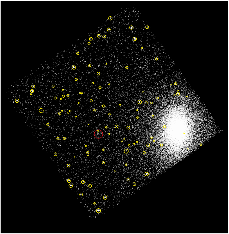
Figure 1.— Detected sources in the Chandra ACIS-I field of A1413. Yellow circles mark point sources. The only detectable extended X-ray source (other than A1413) is marked by the red circle. ACIS-I field of view is $16^{\prime}\times 16^{\prime}$.

The surface brightness profiles are measured in the 0.7–2 keV energy band, which provides an optimal ratio of the cluster and background flux in Chandra data. The blank-field background is subtracted from the cluster images, and the result is flat-fielded using exposure maps that include corrections for CCD gaps and bad pixel, but do not include any spatial variations of the effective area. We then subtract any small uniform component corresponding to adjustments to the soft X-ray foreground that may be required (see Paper I for details of background modeling). This correction is done separately for the back-illuminated (BI) and front-illuminated (FI) CCDs because they have very different low-energy effective area.

We then extracted the surface brightness profiles in narrow concentric annuli ($r_{\text{out}}/r_{\text{in}}=1.05$) centered on the cluster X-ray peak and computed the area-averaged Chandra effective area for each annulus (see Paper I for details on calculating the effective area). Using the effective area and observed projected temperature and metallicity as a function of radius, we converted Chandra count rate in the 0.7–2 keV band into integrated emission measure, $\mathit{EM}=\int n_{e}\,n_{p}\,dV$, within the cylindrical shell. We have verified that these “physical” cluster brightness profiles derived from BI and FI CCDs are always in excellent agreement in the overlapping radial range. The profiles from both CCD sets and different pointings were combined using the statistically optimal weighting. Poisson uncertainties of the original X-ray data were propagated throughout this procedure.

For lower-redshift clusters in our sample, the statistical accuracy of the surface brightness at large radii is limited mostly by the Chandra field of view. The analysis in such cases can benefit from also using data from the ROSAT PSPC pointed observations. We used flat-fielded ROSAT images in the 0.7–2 keV band produced using S. Snowden’s software (Snowden et al., 1994) and reduced as described in Vikhlinin et al. (1999). ROSAT surface brightness profiles were converted to projected emission measure and were used as a second independent dataset in modeling the gas density distribution. We did not use the ROSAT data in the central $2^{\prime}$ from the cluster center, because this region can be affected by the PSPC angular resolution ($\sim 25^{\prime\prime}$ FWHM). At larger radii, we always find excellent agreement between Chandra and ROSAT PSPC surface brightness data (an example is shown in Fig. 2). Below, we used the combined Chandra and ROSAT analysis for those clusters with sufficiently deep PSPC exposures — A133, A262, A478, A1795, A1991, A2029, and MKW4.

3. Modeling of temperature and surface brightness profiles

We model the observed X-ray surface brightness and projected temperature profiles using the following general approach. The 3D profiles of gas density and temperature are represented with analytic functions which are smooth, but have freedom to describe a wide range of the possible profiles. The models are projected along the line of sight and fit to the data. The best fit 3D model is used to derive all interesting cluster parameters, such as the total gravitating mass. Measurement uncertainties for all quantities are estimated using Monte-Carlo simulations in which random statistical errors are added to the data and the full analysis is repeated using these simulated data as an input.

Reliability of this modeling approach was tested by applying our Chandra data analysis procedures to “observations” of clusters from high-resolution numerical simulations (Nagai et al., in preparation). This analysis demonstrated that the three-dimensional gas density and temperature profiles of relaxed clusters are reconstructed within a few percent.

Table 2Best Fit Parameters for Gas Density Profiles

Cluster	$r_{\text{det}}$	$n_{0}$	$r_{c}$	$r_{s}$		$\beta$	$\varepsilon$	$n_{02}$	$r_{c2}$	$\beta_{2}$	ROSAT
	(kpc)	$10^{-3}$ cm-3	(kpc)	(kpc)				$10^{-1}$ cm-1
A133	1100	02.968	142.7	1423.3	0.996	0.575	5.000	0.276	33.44	0.980	+
A262	450	03.434	45.2	350.8	1.674	0.333	1.806	$\cdots$	$\cdots$	$\cdots$	+
A383	800	07.000	115.2	422.3	2.018	0.583	0.740	1.014	00.08	1.000	$\cdots$
A478	2000	08.169	177.1	3148.2	1.493	0.715	5.000	0.584	24.00	1.000	+
A907	1300	06.257	136.9	1885.1	1.554	0.594	4.986	$\cdots$	$\cdots$	$\cdots$	$\cdots$
A1413	1800	05.526	186.3	2077.1	1.217	0.651	4.991	$\cdots$	$\cdots$	$\cdots$	$\cdots$
A1795	1500	14.993	72.8	1030.8	1.060	0.545	3.474	$\cdots$	$\cdots$	$\cdots$	+
A1991	1000	09.373	44.4	998.2	1.516	0.501	5.000	0.999	05.00	1.165	+
A2029	2250	16.469	80.7	870.6	1.131	0.539	1.650	3.741	05.00	1.000	+
A2390	2500	03.069	353.6	1200.0	1.917	0.696	0.240	$\cdots$	$\cdots$	$\cdots$	$\cdots$
RXJ 1159+5531	600	00.198	613.8	961.5	1.762	1.215	4.939	0.416	12.66	1.000	$\cdots$
MKW4	550	00.280	488.6	1081.6	1.628	1.224	0.000	0.189	11.08	0.661	+
USGC S152	300	17.450	8.1	467.5	2.644	0.453	3.280	$\cdots$	$\cdots$	$\cdots$	$\cdots$

Note. — Derived densities and radii scale with the Hubble constant as $h^{1/2}$ and $h^{-1}$, respectively.

3.1. Gas Density Model

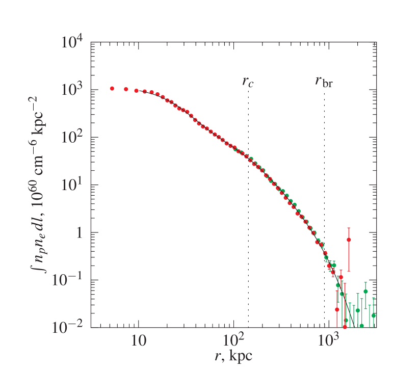
Figure 2.— Observed projected emissivity profile for A133. Chandra and ROSAT PSPC data are shown in red and green, respectively. Solid line shows the best fit to the 3D gas density model (eq. [3]). The slope of the emissivity profile steepens by $1$ at radius $r_{\text{br}}=r_{s}(\varepsilon-1)^{-1/\gamma}$.

The analytic expression we use for the 3D gas density distribution is obtained by modifying the traditionally used $\beta$-model (Cavaliere & Fusco-Femiano, 1978). Modifications are designed to represent essential features of the observed X-ray surface brightness profiles. Gas density in the centers of relaxed clusters, such as ours, usually has a power law-type cusp instead of a flat core and so the first modification is

$$\frac{n_{0}^{2}}{(1+r^{2}/r_{c}^{2})^{3\beta}}\quad\longrightarrow\quad\frac{n_{0}^{2}\;(r/r_{c})^{-\alpha}}{(1+r^{2}/r_{c}^{2})^{3\beta-\alpha/2}}.$$ (1)

This model was also used by, e.g., Pointecouteau et al. (2004).

At large radii, the observed X-ray brightness profiles often steepen at $r>0.3\,r_{200}$ relative to the power law extrapolated from smaller radii (Vikhlinin et al., 1999). This change of slope can be modeled as

$$\frac{n_{0}^{2}}{(1+r^{2}/r_{c}^{2})^{3\beta}}\quad\longrightarrow\quad\frac{n_{0}^{2}}{(1+r^{2}/r_{c}^{2})^{3\beta}}\,\frac{1}{(1+r^{\gamma}/r_{s}{}^{\gamma})^{\varepsilon/\gamma}},$$ (2)

where the additional term describes a change of slope by $\varepsilon$ near the radius $r_{s}$ and the parameter $\gamma$ controls the width of the transition region. Finally, we add a second $\beta$-model component with small core-radius to increase modeling freedom near the cluster centers. The complete expression for the emission measure profile is

$$\begin{split}n_{p}\,n_{e}=n_{0}^{2}\;\frac{(r/r_{c})^{-\alpha}}{(1+r^{2}/r_{c}^{2})^{3\beta-\alpha/2}}\;&\frac{1}{(1+r^{\gamma}/r_{s}{}^{\gamma})^{\varepsilon/\gamma}}\\ &+\frac{n_{02}^{2}}{(1+r^{2}/r_{c2}^{2})^{3\beta_{2}}}.\end{split}$$ (3)

All our clusters can be fit adequately by this model with a fixed $\gamma=3$. All other parameters were free. The only constraint we used to exclude unphysically sharp density breaks was $\varepsilon<5$. The analytic model [3] has great freedom and can fit independently the inner and outer cluster regions. This is important for avoiding biases in the mass measurements at large radii and also for more realistic uncertainty estimates. The best-fit model for the observed surface brightness in A133 is shown by a solid line in Fig. 2.

Parameters in eq. [3] are strongly correlated and therefore their individual values are degenerate. This is not a problem because our goal is only to find a smooth analytic expression for the gas density which is consistent with the observed X-ray surface brightness throughout the radial range of interest.

3.2. Temperature Profile Model

Several previous studies used a polytropic law, $T(r)\propto[\rho_{\text{gas}}(r)]^{\gamma-1}$, to model non-constant cluster temperature profiles (Markevitch et al., 1999; Finoguenov et al., 2001; Pratt & Arnaud, 2002). We take a different approach because the polytropic model is in fact a poor approximation of the temperature profiles at large radii (Markevitch et al., 1998; De Grandi & Molendi, 2002), which is apparent in our more accurate Chandra measurements.

The projected temperature profiles for all our clusters show similar behavior (see Fig. 15 in Paper I and Fig. 3–15 below). The temperature has a broad peak near 0.1–0.2 of $r_{200}$ and decreases at larger radii in a manner consistent with the results of earlier ASCA and Beppo-SAX observations (Markevitch et al., 1998; De Grandi & Molendi, 2002), reaching approximately 50% of the peak value near $0.5\,r_{200}$. There is also a temperature decline towards the cluster center probably because of the presence of radiative cooling. We construct an analytic model for the temperature profile in 3D, in such a way that it can describe these general features. Outside the central cooling region, the temperature profile can be adequately represented as a broken power law with a transition region:

$$t(r)=\frac{(r/r_{t})^{-a}}{(1+(r/r_{t})^{b})^{c/b}}.$$ (4)

The temperature decline in the central region in most clusters can be described as

$$t_{\text{cool}}(r)=(x+T_{\text{min}}/T_{0})/(x+1),\quad x=(r/r_{\text{cool}})^{a_{\text{cool}}},$$ (5)

(Allen, Schmidt & Fabian, 2001b). Our final model for the 3D temperature profile is the product of eq. [4] and [5],

$$T_{\mathrm{3D}}(r)=T_{0}\times t_{\text{cool}}(r)\times t(r).$$ (6)

Our model has great functional freedom (9 free parameters) and can adequately describe almost any type of smooth temperature distribution in the radial range of interest.

This model is projected along the line of sight to fit the observed projected temperature profile. This projection requires proper weighting of multiple temperature components. We use the algorithm described in Vikhlinin (2005) that very accurately predicts the single-temperature fit to multi-component spectra over a wide range of temperatures. The inputs for this algorithm are the 3D profiles of the gas temperature, density, and metallicity. The only missing ingredient in our case is the 3D metallicity profile. We use instead the projected metallicity distributions presented in Paper I. The difference between the projected and 3D abundance profiles leads to very small corrections in the calculation of the project temperature that are negligible for our purposes. We also note that the 3D temperature fit at large radii is rather insensitive to the choice of weighting algorithm. For example, we tested the commonly used method of weighting $T$ with the square of the gas density and obtained very similar results. The primary reason for stability of the $T_{\text{proj}}$ calculations is that the ICM emissivity is a strongly decreasing function of radius and most of the emission observed at a projected distance $b$ comes from a narrow radial range near $r=b$.

In several cases, the cluster X-ray brightness is detected beyond the outer boundary of the Chandra temperature profile. Typical examples are A262 where the ROSAT PSPC profile extends to $50^{\prime}$, well beyond the Chandra FOV, and A383 where the X-ray brightness is detectable in the Chandra image to 1300 kpc, while the temperature profile is sufficiently accurate only within the central 750 kpc. Detection of ICM emission at large radii sets a lower limit to the temperature and thus provides additional information for the $T(r)$ modeling. We required that the 3D temperature model exceeds 0.5 keV at $r=r_{\text{det}}$, the radius where the X-ray brightness is at least $3\sigma$ significant ($r_{\text{det}}$ are reported in Table 1).

We excluded from the fit the data within the inner cutoff radius, $r_{\text{min}}$ (listed in Table 1), which was chosen to exclude the central temperature bin (10–20 kpc) because the ICM is likely to be multi-phase at these small radii. In A133 and A478, $r_{\text{min}}$ was increased to exclude substructures associated with activity of the central AGN. The cutoff radius was increased also in A1795, A2390, and USGC S152, because our analytic model is a poor fit to the inner temperature profile in these clusters. The choice of $r_{\text{min}}$ is unimportant because we are primarily interested in the cluster properties at large radii.

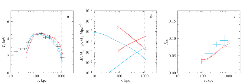
Figure 3.— Results for A133. (a) — Temperature profile. Observed projected temperatures are shown by crosses. Solid red and blue lines show the best fit 3D model and the corresponding projected profile, respectively. Dotted lines indicate the 68% CL uncertainty interval obtained from Monte-Carlo simulations (see text). Models are shown in the radial range $r_{\text{min}}-r_{\text{det}}$ (see text). (b) — Mass and density profiles. $M(r)$ increases with radius and $\rho(r)$ decreases. Red and blue lines show results for the total mass and gas mass, respectively. (c) — Gas mass fraction as a function of radius. Lines show the enclosed $f_{\text{gas}}=M_{\text{gas}}(<r)/M_{\text{tot}}(<r)$. The local gas fraction ($\rho_{\text{gas}}/\rho_{\text{tot}}$) in the radial range directly covered by the Chandra temperature data is shown by crosses. The vertical line shows the radius $r_{500}$ derived from the best fit mass model.

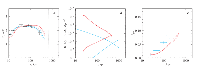
Figure 4.— Results for A262. See caption to Fig. 3.

3.3. Uncertainties

Our analytic models for the gas density and temperature profiles have many free parameters and strong intrinsic degeneracies between parameters. Therefore, uncertainty intervals for all quantities of interest were obtained from Monte-Carlo simulations. The simulated data were realized by scattering the observed brightness and temperature profiles according to a Gaussian distribution with a dispersion equal to measurement uncertainties. The surface brightness and temperature models were fit to the simulated data and the full analysis repeated. The uncertainty on all quantities of interest were obtained by analyzing the distribution derived from 1000–4000 simulated profiles we generated for each cluster.

3.4. Mass Derivation

Given 3D models for the gas density and temperature profiles, the total mass within the radius $r$ can be estimated from the hydrostatic equilibrium equation (e.g., Sarazin, 1988):

$$M(r)=-3.71\times 10^{13}\,M_{\odot}\,T(r)\;r\left(\frac{d\,\log\rho_{g}}{d\,\log r}+\frac{d\,\log T}{d\,\log r}\right),$$ (7)

where $T$ is in units of keV and $r$ is in units of Mpc. Given $M(r)$, we can calculate the total matter density profile, $\rho(r)=(4\pi r^{2})^{-1}\,dM/dr$. We also compute the total mass at several overdensity levels, $\Delta$, relative to the critical density at the cluster redshift, by solving equation

$$M_{\Delta}(r_{\Delta})=\Delta\,4/3\,\pi\,r_{\Delta}^{3}\,\rho_{c}(z),$$ (8)

(see, e.g., White 2001 for discussion of different cluster mass definitions).

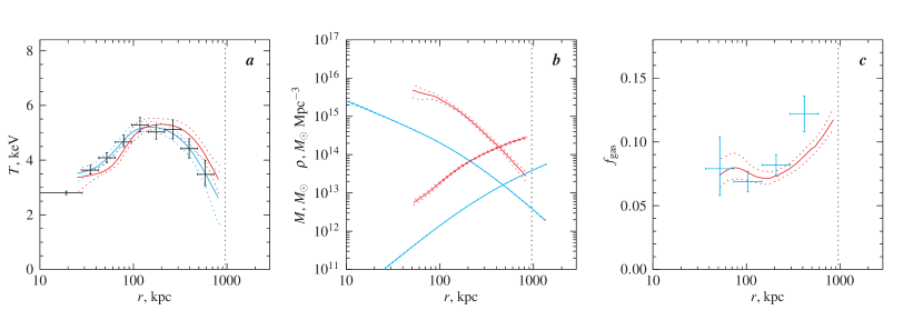
Figure 5.— Results for A383. See caption for Fig. 3.

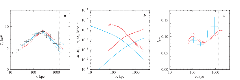
Figure 6.— Results for A478. See caption for Fig. 3.

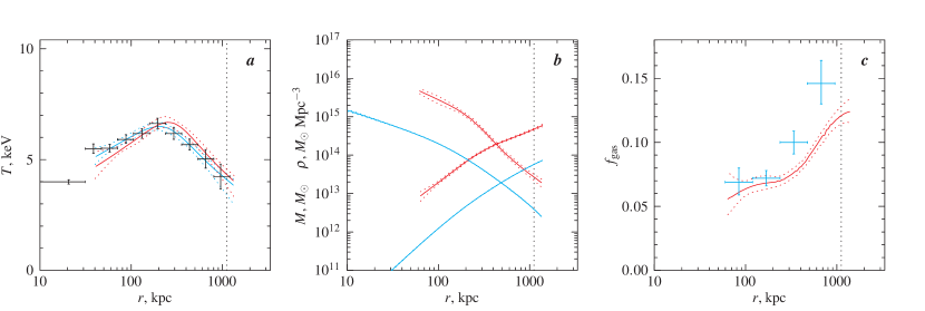
Figure 7.— Results for A907. See caption for Fig. 3.

The ICM particle number density profile is given directly by the analytic fit to the projected emission measure profile (§ 3.1) and it is easily converted to the gas density. For the cosmic plasma with the He abundance from Anders & Grevesse (1989), $\rho_{g}=1.252\,m_{p}\,(n_{p}n_{e})^{1/2}$.

The total mass derived from eq. [7] is a complex combination of parameters which define our $T(r)$ and $\rho_{g}(r)$ models. Its uncertainties are best derived via Monte-Carlo simulations as described in § 3.3. We used the best fit $T(r)$ model obtained for each realization of the temperature profile to compute all quantities of interest ($M_{\Delta}$, $M_{g}$, gas mass fraction, etc.). The peak in the obtained distribution corresponds the most probable value (“best fit”) and the region around the peak containing 68% of all realizations is the 68% CL uncertainty interval.

Our analytic model for $T(r)$ allows very steep gradients. In some cases, such profiles are formally consistent with the observed projected temperatures because projection washes out steep gradients. However, large values of $dT/dr$ often lead to unphysical mass estimates, for example the profiles with $\rho<0$ at some radius. We eliminated this problem in the Monte-Carlo simulations by accepting only those realizations in which the best-fit $T(r)$ leads to $\rho_{\text{tot}}>\rho_{\text{gas}}$ in the radial range covered by the data, $r_{\text{min}}<r<r_{\text{det}}$. Finally, we checked that the temperature profiles corresponding to the mass uncertainty interval are all convectively stable, $d\ln T/d\ln\rho_{g}<2/3$.

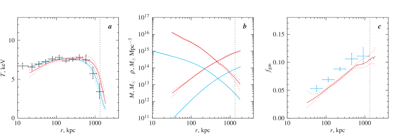
Figure 8.— Results for A1413. See caption for Fig. 3.

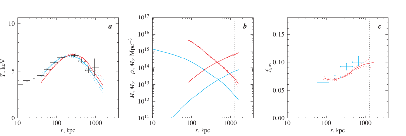
Figure 9.— Results for A1795. See caption for Fig. 3.

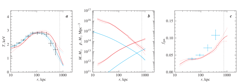
Figure 10.— Results for A1991. See caption for Fig. 3.

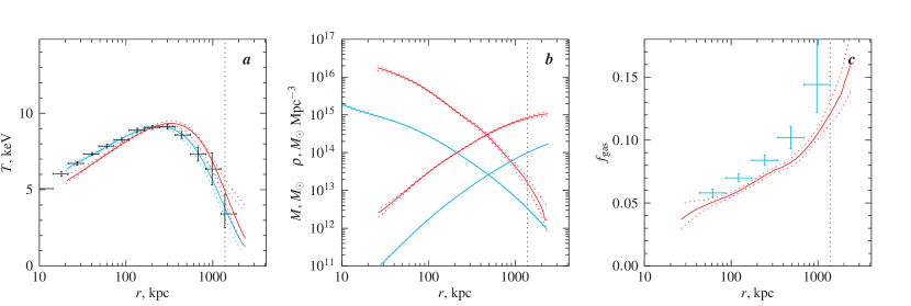
Figure 11.— Results for A2029. See caption for Fig. 3.

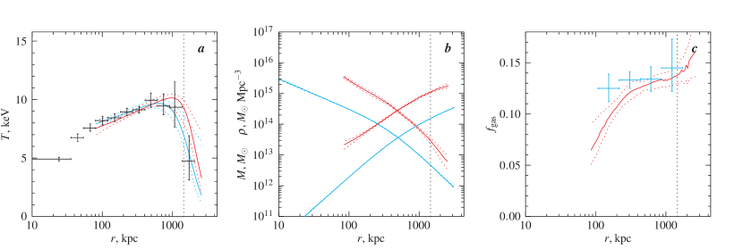
Figure 12.— Results for A2390. See caption for Fig. 3.

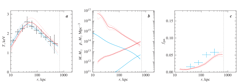
Figure 13.— Results for RXJ 1159+5531. See caption for Fig. 3.

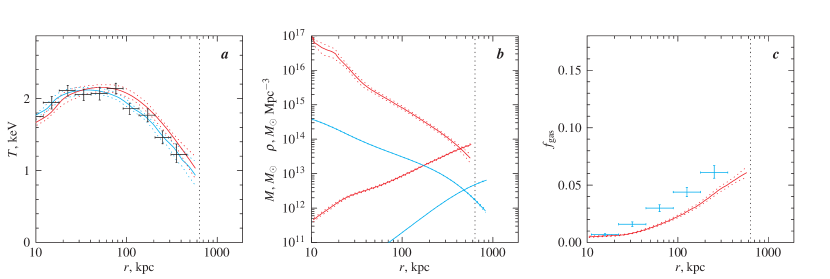
Figure 14.— Results for MKW4. See caption for Fig. 3.

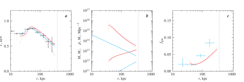
Figure 15.— Results for USGC S152. See caption for Fig. 3.

3.5. Average Temperatures

We also computed average temperatures for each cluster using different weightings of the 3D temperature models. The temperatures were averaged in the radial range $70\,\text{kpc}<r<r_{500}$. The central 70 kpc were excluded because temperatures at these radii can be strongly affected by radiative cooling and thus not directly related to the depth of the cluster potential well. The averages we compute are:

$T_{mg}$ — weighted with $\rho_{\text{gas}}(r)$. $T_{mg}$ is needed, e.g., to compute the integrated SZ (Sunyaev & Zeldovich, 1972) signal. $T_{mg}$ should be more directly related to the cluster mass than X-ray emission-weighted temperatures.

$T_{\text{spec}}$ — a value that would be derived from the single-temperature fit to the total cluster spectrum, excluding the central region. $T_{\text{spec}}$ is obtained by integrating a combination of $T(r)$ and $\rho_{\text{gas}}^{2}(r)$ as described in Vikhlinin (2005). $T_{\text{spec}}$ is one of the primary X-ray observables.

Measurement uncertainties for the average temperatures are derived via Monte-Carlo simulations (§ 3.3 and 3.4).

4. Results for individual clusters

Best fit parameters for the gas density distribution are listed in Table 2. We do not provide measurement uncertainties for the individual parameters because they are strongly degenerate. Monte-Carlo simulations show that for each cluster, the statistical uncertainties of the gas density are below 9% everywhere in the radial range $5\,\text{kpc}-r_{\text{det}}$. However, extrapolations of the gas density far beyond $r_{\text{det}}$ are unreliable. The main derived cluster parameters are reported in Table 3, and temperature, mass, and gas fraction profiles for individual clusters are presented in Fig. 3–15.

The observed temperature profile and the best-fit models are shown in panels (a). The models are shown in the radial range $r_{\text{min}}-r_{\text{det}}$. Note that our analytic function successfully describes a wide range of shapes for the observed temperature profiles and the corresponding projected profiles (shown by blue lines) are always excellent fits to the data. The 3D models (red lines) go above the data in the outer region, and below the data in the center — just as expected from projection of the temperature gradients along the line of sight.

Dotted lines show 68% CL uncertainties for the model at each radius derived from Monte-Carlo simulations. The uncertainty intervals are smaller than the errorbars of the raw measurements because the model effectively smoothes the data over 3–4 adjacent bins (and therefore uncertainties in the neighboring bins are correlated). However, the difference is not very large and the derived uncertainties are clearly realistic in the sense that they include a typical range of smooth models that could be drawn through the data.

Panels (b) present the derived density and enclosed mass profiles. Results for the total and gas masses are shown by red and blue lines, respectively. $M(r)$ increases with radius and $\rho(r)$ decreases. The derived total mass profile is used to estimate the radius, $r_{500}$ (vertical dotted lines). If $r_{500}$ is outside the radial range covered by the X-ray data, we find it from extrapolation of our best fit gas density and/or temperature models. Large extrapolations are required only for A262, RXJ 1159+5531, and USGC S152. In other cases, Chandra temperature measurements extend almost to $r_{500}$ or beyond.

Dotted lines show 68% CL uncertainties for the mass and density derived from Monte-Carlo simulations for a subset of physically meaningful realizations (see § 3.4). Uncertainties are shown also for the gas mass but they are very small and almost indistinguishable from the best fit model in these plots.

Gas fraction profiles are presented in panels (c). The enclosed gas fraction is shown by red lines. The local gas fraction, $\rho_{\text{gas}}/\rho_{\text{tot}}$, in the radial range directly covered by the Chandra temperature data, is shown by crosses.

Abell 2390 deserves a special note. Its deep Chandra image reveals large-scale cavities in the X-ray surface brightness extending $\sim 400$ kpc from the center where a sharp break in the surface brightness profile was reported by Allen et al. (2001a). The cavities are likely produced by bubbles of radio plasma emitted by the central AGN, as observed in several other clusters (McNamara et al., 2005). The ICM in the central region is not spherically symmetric nor expected to be in hydrostatic equilibrium. This should result in underestimation of the total mass and overestimation of the gas mass. The results at small radii for A2390 should be treated with caution. There are no detectable structures outside 500 kpc and so the results at large radii (e.q., at $r_{500}$) should be reliable.

5. Average Temperature Profile

We noted in Paper I that the temperature profiles for our clusters are self-similar when scaled to the same overdensity radius, in good agreement with the earlier studies by Markevitch et al. (1998) and De Grandi & Molendi (2002). We return to this subject here because results for individual clusters can be compared more accurately using the reconstructed 3-dimensional temperature profiles and the overdensity radii determined from the mass model rather than estimated from the average temperatures as in Paper I.

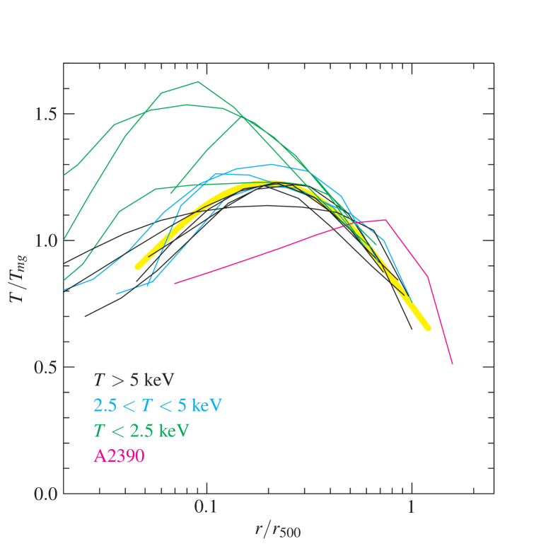
Figure 16.— Scaled 3-dimensional temperature profiles. The mean temperature is the gas mass-weighted average. The thick yellow line shows an approximation to the average profile for $T>2.5$ keV clusters (eq. [9]).

Figure 16 shows the reconstructed 3-dimensional temperature profiles, normalized to the gas mass-weighted average temperature, $T_{mg}$, and plotted as a function of $r/r_{500}$. The model for each cluster is plotted in the radial range directly covered by the Chandra spectral measurements and our 3D modeling, from $r_{\text{min}}$ to the outer bin in Fig. 3a–15a. We normalize the profiles to the gas mass-weighted temperature because it is less sensitive than, e.g., $T_{\text{spec}}$ to the properties of the central regions where the ICM temperature can be significantly affected by non-gravitational processes.

Table 3Masses, Average Temperatures, Concentration parameter, Gas Fractions

Cluster	$r_{500}$	$T_{\text{spec}}$	$T_{\text{mg}}$	$c_{500}$	$M_{2500}$	$M_{500}$	$f_{\text{g, 2500}}$	$f_{\text{g, 500}}$	$f_{\text{g, 2500-500}}$
	(kpc)	(keV)	(keV)		($10^{14}\,M_{\odot}$)	($10^{14}\,M_{\odot}$)
A133	$998\pm 37$	$4.15\pm 0.07$	$3.68\pm 0.11$	$3.31\pm 0.27$	$1.24\pm 0.08$	$3.14\pm 0.36$	$0.065\pm 0.002$	$0.084\pm 0.006$	$0.095^{+0.014}_{-0.013}$
A262	$663\pm 19$	$2.08\pm 0.06$	$1.92\pm 0.09$	$3.58\pm 0.27$	$0.34\pm 0.05$	$\cdots$	$0.067\pm 0.003$	$\cdots$	$\cdots$
A383	$956\pm 33$	$4.80\pm 0.12$	$4.36\pm 0.18$	$4.36\pm 0.35$	$1.68\pm 0.15$	$3.10\pm 0.32$	$0.090\pm 0.005$	$0.122\pm 0.007$	$0.149^{+0.035}_{-0.024}$
A478	$1359\pm 60$	$7.95\pm 0.14$	$7.34\pm 0.32$	$3.75\pm 0.28$	$4.23\pm 0.26$	$7.83\pm 1.04$	$0.096\pm 0.004$	$0.118\pm 0.011$	$0.130^{+0.031}_{-0.026}$
A907	$1117\pm 31$	$5.96\pm 0.08$	$5.44\pm 0.13$	$3.56\pm 0.31$	$2.30\pm 0.16$	$4.71\pm 0.39$	$0.090\pm 0.003$	$0.121\pm 0.005$	$0.145^{+0.020}_{-0.016}$
A1413	$1339\pm 48$	$7.38\pm 0.12$	$6.76\pm 0.20$	$3.06\pm 0.16$	$3.08\pm 0.19$	$7.78\pm 0.83$	$0.092\pm 0.003$	$0.104\pm 0.007$	$0.112^{+0.014}_{-0.014}$
A1795	$1283\pm 46$	$6.10\pm 0.06$	$5.52\pm 0.11$	$3.73\pm 0.17$	$2.66\pm 0.15$	$6.57\pm 0.69$	$0.088\pm 0.003$	$0.098\pm 0.007$	$0.099^{+0.017}_{-0.013}$
A1991	$753\pm 39$	$2.59\pm 0.06$	$2.23\pm 0.09$	$4.66\pm 0.32$	$0.60\pm 0.07$	$1.28\pm 0.20$	$0.068\pm 0.004$	$0.099\pm 0.009$	$0.103^{+0.050}_{-0.017}$
A2029	$1380\pm 31$	$8.46\pm 0.09$	$7.59\pm 0.19$	$4.13\pm 0.24$	$4.41\pm 0.23$	$8.29\pm 0.79$	$0.090\pm 0.003$	$0.121\pm 0.007$	$0.144^{+0.033}_{-0.021}$
A2390	$1448\pm 49$	$8.90\pm 0.17$	$9.35\pm 0.39$	$1.65\pm 0.18$	$3.50\pm 0.28$	$10.88\pm 1.05$	$0.127\pm 0.005$	$0.138\pm 0.008$	$0.141^{+0.014}_{-0.014}$
RXJ 1159+5531	$695\pm 60$	$1.80\pm 0.10$	$1.58\pm 0.09$	$1.89\pm 0.35$	$0.31\pm 0.04$	$\cdots$	$0.042\pm 0.002$	$\cdots$	$\cdots$
MKW4	$635\pm 27$	$1.65\pm 0.05$	$1.40\pm 0.05$	$2.69\pm 0.17$	$0.30\pm 0.03$	$0.74\pm 0.09$	$0.044\pm 0.002$	$0.063\pm 0.005$	$0.073^{+0.014}_{-0.013}$
USGC S152	$\cdots$	$0.69\pm 0.02$	$0.59\pm 0.03$	$\cdots$	$0.07\pm 0.00$	$\cdots$	$0.043\pm 0.001$	$\cdots$	$\cdots$

Note. — The derived quantities scale with the Hubble constant as $r_{500}\propto h^{-1}$, $M\propto h^{-1}$, $f_{\text{gas}}\propto h^{-3/2}$.

At $r\gtrsim 0.05\,r_{500}$, the scaled 3-dimensional temperature for all but one of our $T>2.5$ keV clusters are within $\pm 15\%$ from the average profile which can be approximated with eq. [6],

$$\frac{T(r)}{T_{mg}}=1.35\;\frac{(x/0.045)^{1.9}+0.45}{(x/0.045)^{1.9}+1}\;\frac{1}{(1+(x/0.6)^{2})^{0.45}},$$ (9)

where $x=r/r_{500}$. This average model is shown in Fig.16 by thick yellow line. The only deviation is A2390, in which the inner temperature profile and overall normalization appear to be distorted by activity of the central AGN (see above). The profiles of the low-temperature clusters, $T<2.5$ keV (green lines in Fig. 16), follow the average profile at $r\gtrsim 0.3\,r_{500}$ but are significantly different and show large scatter at small radii. They show a stronger temperature increase to the center, and the central cooler regions seem to be confined to a smaller fraction of the virial radius than in the more massive clusters.

The observed radial temperature variations imply that the average cluster temperature cannot be defined uniquely. A possible difference between different definitions (spectroscopic, emission-weighted, gas mass-weighted etc.) should be kept in mind. Also, the aperture size used for integration of the X-ray spectrum is important. Our average 3-dimensional profile [9] implies the following approximate relation between the peak, spectroscopic average, and gas mass-weighted temperatures (all measured in the radial range $70~{}\text{kpc}-r_{500}$):

$$T_{\text{peak}}:T_{\text{spec}}:T_{mg}=1.21:1.11:1.$$ (10)

Comparing our temperature profiles with the compilation of XMM-Newton results presented in Arnaud et al. (2005), we note a general agreement at small radii. However, the results at large radii seem to be different — the temperature decline is generally not present in these XMM-Newton clusters. Discussion of this discrepancy is beyond the scope of this paper. The arguments for validity of our measurements and detailed comparison with the Arnaud et al. results for several clusters in common can be found in Paper I.

6. Total and Gas Density Profiles

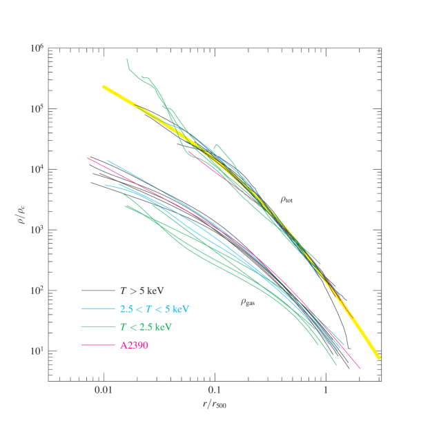
Figure 17.— Scaled density profiles. Total density profiles are plotted within the radial range covered by the temperature profile. Gas density profiles are extended to $r_{\text{det}}$ (see Table 2). Thick yellow line shows the NFW model with $c_{500}=3$, a typical value for CDM halos in our mass range (§ 6.1, see Fig. 18).

One of the key theoretical predictions of the hierarchical CDM models is the universal density distribution within dark matter halos (Navarro et al., 1996, 1997, hereafter NFW). Specifically, the shape of the radial density profiles of Cold Dark Matter halos is characterized by a gradually changing slope $\alpha=d\log\rho/d\log r$ from $\alpha\approx-1$ in the inner regions to $\alpha\approx-3$ at large radii (Dubinski & Carlberg, 1991, NFW). The profiles are characterized by concentration, $c_{\Delta}$, defined as the ratio of the halo virial radius and the scale radius, $r_{s}$: $c_{\Delta}\equiv r_{\Delta}/r_{s}$. The scale radius is defined as the radius where the logarithmic slope of the density profile is $\alpha=-2$. Concentrations of CDM halos are tightly correlated with the characteristic epoch of object formation (Wechsler et al., 2002). The mean concentration is only a weakly decreasing function of the virial mass, $c_{\Delta}\propto M_{\Delta}^{0.1}$, (Navarro et al., 1997; Bullock et al., 2001; Eke et al., 2001). Therefore, within a limited range of masses, the mean concentration is approximately constant and the density profiles are approximately self-similar.

Such self-similarity is indeed observed in our data. In Fig.17, we plot the derived total density profiles, scaled to $\rho_{c}(z)$, as a function of radius in units of $r_{500}$. The scatter of individual clusters around a mean profile is small and consistent with that found in numerical simulations (see § 6.1 below). The average total density profile in our clusters agrees well with the NFW model with the concentration expected for objects of this mass (thick yellow line in Fig.17).

The $\rho_{\text{tot}}$ profiles for 3 clusters with $T<2.5$ keV have central steepening at $r<0.05\,r_{500}\approx 30$ kpc, which is statistically significant. Such sharp steepening is not expected in purely CDM halos. We associate these components with the stellar material of the central cD galaxies, which start to dominate the total mass at small radii. Indeed, our derived masses within 30 kpc for these objects, $\sim 2\times 10^{12}\,M_{\odot}$ (see Fig.3) are similar to the stellar mass estimates in large central cluster galaxies (e.g., Lin & Mohr, 2004).

Self-similarity is also observed in the ICM distribution at large radii. The lower set of profiles in Fig. 17 shows the gas densities, also scaled to $\rho_{c}(z)$. The scaled gas density near $r_{500}$ is within $\pm 15\%$ of the mean for most clusters. Some of this scatter is caused by uncertainties in the total mass estimates — a typical uncertainty of 3–5% in $r_{500}$ (Table 3) translates into 7–12% scatter in the scaled densities for a typical slope of $\rho_{\text{gas}}(r)$ near $r_{500}$. The scatter in the gas density profiles becomes significantly larger in the inner region, which was already noted in the previous studies (e.g., Neumann & Arnaud, 1999; Vikhlinin et al., 1999).

There is also a trend for lower-temperature clusters to have lower gas densities and flatter profiles in the central region. This trend is responsible for flat gas density slopes derived for galaxy groups and low-mass clusters in the previous analyses using the $\beta$-model approximations (e.g., Helsdon & Ponman, 2000; Finoguenov et al., 2001; Sanderson et al., 2003). However, we observe that at large radii, the gas density in cold clusters approaches the average profile defined by $T>5$ keV clusters. Also, the gas density profiles often steepen at $r\simeq 0.7\,r_{500}$ so that the slopes near $r_{500}$ are similar for all clusters. Further discussion of this issue and its impact on the hydrostatic mass estimates is presented in Appendix A.

Below, we compare the concentration parameters for our $\rho_{\text{tot}}$ profiles with those expected for CDM halos. Comparison of the gas density distributions with the results of numerical simulations will be presented in a future paper.

6.1. Concentration parameters

As discussed above, the $\Lambda$CDM paradigm makes a firm theoretical prediction for concentrations of the dark matter halos. It is interesting to compare our measurements with these predictions. We define the concentration as $c_{500}\equiv r_{500}/r_{s}$ because our mass measurements typically extend to $\sim r_{500}$. The scale radius $r_{s}$ was determined by fitting the NFW model to values of the total density at six radii equally log-spaced in the range $0.05\,r_{500}-r_{\text{det}}$. The range $r<0.05\,r_{500}$ is excluded because at these radii there are separate mass components associated with the stellar material in cD galaxies (see above); such components are found in a similar radial range in numerical simulations, which include cooling and star formation (e.g., Gnedin et al., 2004). The uncertainties for $c_{500}$ are derived from the Monte-Carlo simulations described in § 3. The resulting $c_{500}$ determinations are reported in Table 3 and plotted as a function of measured $M_{500}$ in Fig.18.

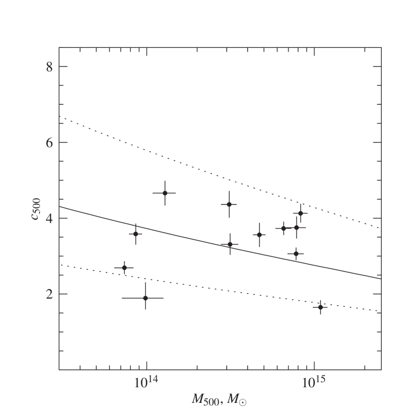
Figure 18.— Concentration parameters of the NFW model, $c_{500}=r_{500}/r_{s}$, as a function of cluster mass. Solid points with error bars are our measurements. Solid line shows the average concentration of CDM halos from simulations by Dolag et al. (2004a). Dotted lines show 2-$\sigma$ scatter of log-normal distribution of concentrations at a fixed mass, found in simulations.

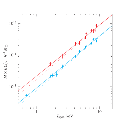
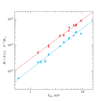
Figure 19.— Total mass within $r_{500}$ (red) and $r_{2500}$ (blue), as a function of X-ray spectroscopic temperature, $T_{\text{spec}}$, and gas mass-weighted temperature, $T_{mg}$. Solid lines show the best fit power laws with parameters listed in Table 4. Dotted lines in the $T_{\text{spec}}$ plot show the best fit relations from Arnaud et al. (2005). Note that $M_{500}$ measurements are not plotted for clusters which required large extrapolations of the temperature profiles (A262, RXJ 1159+5531, USGC S152).

The measurements are compared with the expected $c(M)$ relation suggested by the cluster simulations of Dolag et al. (2004a, see their eq. 13 and Table 2) in the “concordance” $\Lambda$CDM cosmology, $\Omega_{0}=1-\Omega_{\Lambda}=0.3$, $\sigma_{8}=0.9$ (solid line in Fig. 18). Note that we converted the concentrations and masses from the definitions used by Dolag et al. to $c_{500}$ and $M_{500}$ used in our analysis (e.g., Hu & Kravtsov, 2003). We also show (dotted lines) the 2-$\sigma$ scatter of concentrations typically found in numerical simulations, $\sigma_{\ln c}=0.22$ (Jing, 2000; Bullock et al., 2001; Wechsler et al., 2002; Tasitsiomi et al., 2004; Dolag et al., 2004a).

Clearly, both the typical values and scatter of concentrations determined for our clusters are in general agreement with the simulation results. It can be argued that for massive clusters, most of our measurements are slightly higher than the theoretical average. If this effect is real, it can be caused by several factors. First, our sample contains only a highly relaxed sub-population of galaxy clusters which are expected to sample the high tail of the concentration distribution (Wechsler et al., 2002). Second, radiative cooling of baryons and the associated galaxy formation are expected to modify the density profiles of parent CDM halos. These processes are expected to steepen the mass distribution in the inner regions of clusters, due to buildup of the central cluster galaxy (Gnedin et al., 2004) and make the mass distribution considerably more spherical on scales as large as $r_{500}$ (Kazantzidis et al., 2004). The amplitude of this effect, determined from a sample of simulated clusters described in Kravtsov, Nagai & Vikhlinin (2005) with two additional massive Coma-size objects, is $\Delta c_{500}=0.5-1$ (Kravtsov et al., in preparation). This is similar to the possible systematic enhancement of concentration we observe for $M>2\times 10^{14}\,M_{\odot}$ clusters.

Table 4Power Law Fit to Mass-Temperature Relation

	$T_{\text{spec}}$				$T_{\text{mg}}$
Overdensity	$M_{5}$,  $h^{-1}M_{\odot}$	$r_{5}$,  $h^{-1}$ Mpc			$M_{5}$,  $h^{-1}M_{\odot}$	$r_{5}$,  $h^{-1}$ Mpc
$\Delta=500$	$(2.93\pm 0.16)\times 10^{14}$	$0.796\pm 0.015$	$1.61\pm 0.11$		$(3.41\pm 0.18)\times 10^{14}$	$0.837\pm 0.015$	$1.51\pm 0.10$
$\Delta=2500$	$(1.28\pm 0.05)\times 10^{14}$	$0.354\pm 0.005$	$1.64\pm 0.06$		$(1.48\pm 0.07)\times 10^{14}$	$0.371\pm 0.006$	$1.58\pm 0.07$

Note. — We use a power law fit of the form $h(z)\,M=M_{5}\times(T/5\,\text{keV})$, where $M=M_{500}$ or $M_{2500}$ and temperatures are either X-ray spectral or gas mass-weighted averages (see § 3.5). Scaling of the corresponding overdensity radii with temperature is of the form [13].

The main conclusion from this analysis is that there is good overall agreement between theoretical expectations and the measured concentration parameters in our cluster sample. A similar conclusion was reached by Pointecouteau et al. (2005) from the XMM-Newton analysis of 10 clusters.

7. Mass-Temperature Relation

A tight relation between the cluster temperature and total mass is expected on theoretical grounds, which is indeed observed at least for the hydrostatic mass estimates (Nevalainen et al., 2000; Horner et al., 1999; Finoguenov et al., 2001; Xu et al., 2001; Sanderson et al., 2003). Recent determinations of the $M-T$ relation from Chandra and XMM-Newton observations were presented in Allen et al. (2001b) and Arnaud et al. (2005), respectively (Allen et al. derived masses for the critical overdensity 2500 and Arnaud et al. also presented measurements at larger radii, including extrapolation to $r_{200}$). We can significantly improve over these previous measurements because our temperature profiles extend to large radii and therefore we do not use simplifying assumptions such as that $T(r)$ is constant or polytropic. Also, we have high-quality X-ray surface brightness measurements for all clusters at radii well beyond $r_{500}$, and do not use the common $\beta$-model approximation to derive the gas densities.

We measure total masses for two often-used critical overdensity levels, $\Delta=2500$, and $\Delta=500$. The $\Delta=500$ level is particularly useful because it approximately delineates the inner cluster region where the bulk ICM velocities are small and therefore the hydrostatic mass estimates are meaningful (Evrard, Metzler & Navarro, 1996). The corresponding radius, $r_{500}$, is 0.5–0.67 of the virial radius, depending on $\Omega_{m}$ (Eke et al., 1996; Bryan & Norman, 1998). The $\Delta=2500$ overdensity level encompasses the bright central region where X-ray temperature profile measurements are feasible with Chandra even in high-redshift clusters (Allen et al., 2004).

We do not consider the masses for lower overdensities because this would require extrapolation far beyond the radius covered by the Chandra data, and because the ICM is not expected to be fully in hydrostatic equilibrium at large radii. Mass measurements are sometimes extrapolated from the inner region to, e.g., $r_{200}$ assuming the NFW model for the matter density profile. Such extrapolations are highly model-dependent and lead to underestimated measurement uncertainties for $M_{200}$. It is more appropriate to scale the theoretical models to $r_{500}$, where direct measurements are now available. Scaling of mass of CDM halos to any overdensity level is straightforward (Hu & Kravtsov, 2003).

The measured values of $M_{2500}$ and $M_{500}$ are reported in Table 3. We do not compute $M_{500}$ for three clusters for which the temperature profile measurements have to be extrapolated too far (A262, RXJ 1159+5531, and USGC S152). For A2390, $M_{2500}$ should be treated with caution because $r_{2500}$ is near the boundary of the central non-hydrostatic region (see § 4).

In Fig.19, we plot the measured masses as a function of the X-ray spectroscopic and gas mass-weighted temperatures. The self-similar evolution of the normalization of the $M-T$ relation is expected to follow

$$M_{\Delta}/T^{3/2}\propto E(z)^{-1},\quad E(z)=H(z)/H_{0},$$ (11)

(e.g., Bryan & Norman, 1998). Even though the effect of evolution is small within our redshift interval, we applied the corresponding corrections by multiplying the measured masses by $E(z)$ computed for our preferred cosmology, thus “adjusting” all measurements to $z=0$.

We fit the observed $M-T$ relation with a power law,

$$M=M_{5}\,(T/5\,\text{keV}).$$ (12)

The relation is normalized to $T=5$ keV because this is approximately the median temperature for our sample and therefore the estimates for $M_{5}$ and should be nearly independent. The fit is performed using the bisector modification of the Akritas & Bershady (1996, and references therein) linear regression algorithm that allows for intrinsic scatter and nonuniform measurement errors in both variables. The uncertainties were evaluated by bootstrap resampling (e.g., Press et al., 1992), while simultaneously adding random measurement errors to $M$ and $T$.

The best fit slopes and normalizations for different variants of the $M-T$ relations are reported in Table 4. We find flatter slopes ($\alpha\simeq 1.5-1.6$) than many previous studies (typically, $\alpha=1.7-1.8$ when low-temperature clusters were included). Some of the difference can be traced to slightly different definitions of the cluster temperature in individual studies and different procedures for scaling the measurements to $z=0$. However, the major effects are accurate measurements of the temperature gradient at large radii and correct modeling of the steepening in the gas density profiles at large radii. The comparison with other works discussed in detail in Appendix A.

The $M-T$ relation implies the following scaling of the overdensity radii with temperature

$$r_{\Delta}\,h\,E(z)=r_{5}\,(T/5\,\text{keV})^{\alpha/3},$$ (13)

with coefficients $r_{5}$ provided in Table 4.

As seen in Fig.19, the scatter of the individual $M$ and $T$ measurements around the best fit power law approximations is very small. Note that in our case, unlike many previous studies, this is not just a trivial consequence of the approximate similarity of the cluster X-ray surface brightness profiles (Neumann & Arnaud, 1999) because we do not use overly-constrained models for $T(r)$. To characterize the scatter, we compute the rms deviations in mass and subtract the expected contribution from the measurement errors,

$$(\delta M/M)^{2}=\frac{1}{N-2}\sum\frac{(M_{i}-M_{5}(T_{i}/5))^{2}-\Delta M_{i}^{2}}{M_{i}^{2}},$$ (14)

where $\Delta M_{i}$ are measurement errors and $\delta M/M$ is the estimated scatter in the relation (the $1/(N-2)$ factor accounts for 2 degrees of freedom in the power law fit). We find that the observed scatter is consistent with zero, and the 90% upper limits for intrinsic scatter are $\delta M/M\simeq 0.15$ for both $M_{500}$ and $M_{2500}$, and for both definitions of the mean temperature, $T_{\text{spec}}$ and $T_{mg}$. Note the scatter is likely to be larger for the whole cluster population including non-relaxed objects.

Our normalizations of the $M-T$ relation are higher than most of the previous X-ray determinations based on ASCA and ROSAT analyses (see Appendix A for detailed discussion). There is, however, a very good agreement with the XMM-Newton measurements by Arnaud et al. (2005, their results are shown by dotted lines in Fig.19), although this appears to be a result of a chance cancellation of systematic differences between our analyses (Appendix A.2).

Our normalization of the $M-T$ relation is also in good agreement with those derived from recent high-resolution numerical simulations (e.g., Borgani et al., 2004) that attempt to model non-gravitational processes in the ICM (radiative cooling, star formation, feedback from SN). Detailed comparison of our measurements with the results of numerical simulations will be presented elsewhere.

The primary goal of observationally calibrating the $M-T$ relation is for use in fitting cosmological models to the cluster temperature function. Given the good agreement of our results with some other recent measurements (Arnaud et al., 2005) and results of realistic cluster numerical simulations, it is tempting to conclude that observational determinations of the $M-T$ normalization have finally converged to the true value. We, however, caution against direct application of our normalizations to fitting the published cluster temperature functions (Markevitch, 1998; Henry, 2000; Ikebe et al., 2002) for several reasons. First, the definitions of the mean cluster temperature in these papers is not identical to ours. Second, our determination of the $M-T$ relation uses only the most relaxed clusters at the present epoch and it can be significantly different for mergers (Randall et al., 2002). Even for relaxed clusters in the present sample, our analysis neglects potential deviations from hydrostatic equilibrium (e.g., caused by ICM turbulence) or deviations from spherical symmetry. A detailed study of these effects will be presented in Nagai et al. (in preparation); they can lead to $\sim 10\%$ underestimation of the total masses in our analysis (e.g., Evrard et al., 1996; Rasia et al., 2004; Kay et al., 2004; Faltenbacher et al., 2005).

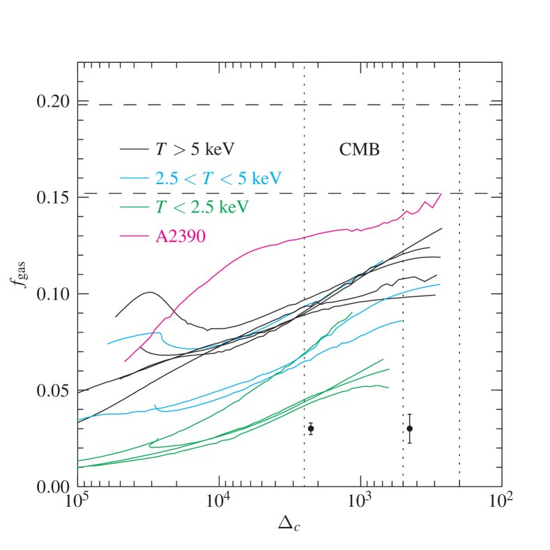
Figure 20.— Enclosed gas fraction as a function of overdensity, defined with respect to the critical density at the cluster redshift. Dashed lines show the range $\Omega_{b}/\Omega_{m}=0.175\pm 0.023$ constrained by CMB observations. Points with error bars show typical measurement uncertainties at two radii.

8. Gas fractions

Finally, we present determinations of the ICM mass fractions in our clusters. Such measurements, especially within a large fraction of the cluster virial radius, are of great cosmological significance because they provide an independent test for $\Omega_{M}$ assuming that the baryon fraction in clusters is close to the cosmic mean (White et al., 1993b).

The derived ICM mass fractions, $f_{\text{gas}}$, as a function of radius are shown for individual clusters in Fig. 3c–15c. We present results for both enclosed gas fractions (continuous lines) and local fractions within several spherical shells (crosses). In almost all clusters there is a significant increase of $f_{\text{gas}}$ with radius, in qualitative agreement with a number of previous measurements that used spatially-resolved temperatures (e.g., Markevitch & Vikhlinin, 1997; Markevitch et al., 1999; Pratt & Arnaud, 2002; Allen et al., 2004).

Comparison of observed gas fractions for individual clusters as a function of overdensity (Fig.20) gives further insights. At $\Delta<10^{4}$, the gas fraction increases with radius as a power law of overdensity. Except for maybe in three clusters, no flattening of $f_{\text{gas}}(r)$ is observed, at least within $r_{500}$. The average ratio of $f_{\text{gas}}$ within $r_{2500}$ and $r_{500}$ is $f_{2500}/f_{500}=0.84$ in massive clusters.

There is also a significant trend of increasing $f_{\text{gas}}$ with cluster mass. The effect is the strongest at small radii, but even within $r_{500}$, $f_{\text{gas}}(M)$ is not constant. In Fig.21, we plot the enclosed gas fractions within $r_{2500}$ and $r_{500}$ as a function of cluster temperature. The gas fraction at $r_{2500}$ increases approximately linearly with temperature from $f_{2500}\simeq 0.04$ for three $T<2$ keV clusters to $f_{2500}\simeq 0.10-0.11$ for the most massive clusters. Another possibility is that there is a flattening at $f_{2500}\simeq 0.09$ at $T>5$ keV and that the measurement for the highest-temperature cluster, A2390, is strongly biased (see § 4). We cannot distinguish these possibilities because of significant object-to-object scatter and the small sample size.

The global baryon fraction in the Universe is constrained by CMB observations to be $\Omega_{b}/\Omega_{m}=0.175\pm 0.023$ (Readhead et al., 2004; Spergel et al., 2003). Therefore, the observed gas fraction within $r_{2500}$, even in the most massive of our clusters, is significantly lower, by a factor of $\sim 0.6$, than the cosmic mean. A similar level of baryonic deficit was previously noted by Ettori (2003) and its systematic variation with mass was obtained indirectly by Arnaud & Evrard (1999) and Mohr et al. (1999). This deficit, and cluster-to-cluster variations of $f_{2500}$ can, at least in part, be explained by conversion of ICM into stars. Contribution of the stars to the total baryon budget should be most important in the cluster centers because of the presence of cD galaxies. Indeed, the largest cD galaxies have K-band luminosities $(1-2)\times 10^{12}\,L_{\odot}$ (Lin & Mohr, 2004). Assuming a stellar mass-to-light ratio in the K-band of $\sim 1$ (Bell et al., 2003), we can estimate that just the cD, not counting other galaxies, can contribute from $0.07$ to $0.01$ to the baryon fraction within $r_{2500}$, depending on the cluster mass. Therefore, the stellar mass in the cluster centers is significant and it should be determined individually in each cluster. Another important process that can affect $f_{\text{gas}}$ in the cluster centers — and otherwise break the self-similarity of the gas properties — is energy output from central AGNs (Nulsen et al., 2005).

The stellar contribution to the total baryon mass and relative energetics of non-gravitational processes should be less important within larger radii. Indeed, we observe that $f_{\text{gas}}$ increases between $r_{2500}$ and $r_{500}$, by factors of 1.2–1.4. Also, the trend of $f_{500}$ with temperature is weaker than that for $f_{2500}$. It is consistent with both a linear increase of $f_{\text{gas}}$ with $T$ and flattening at $T>5$ keV.

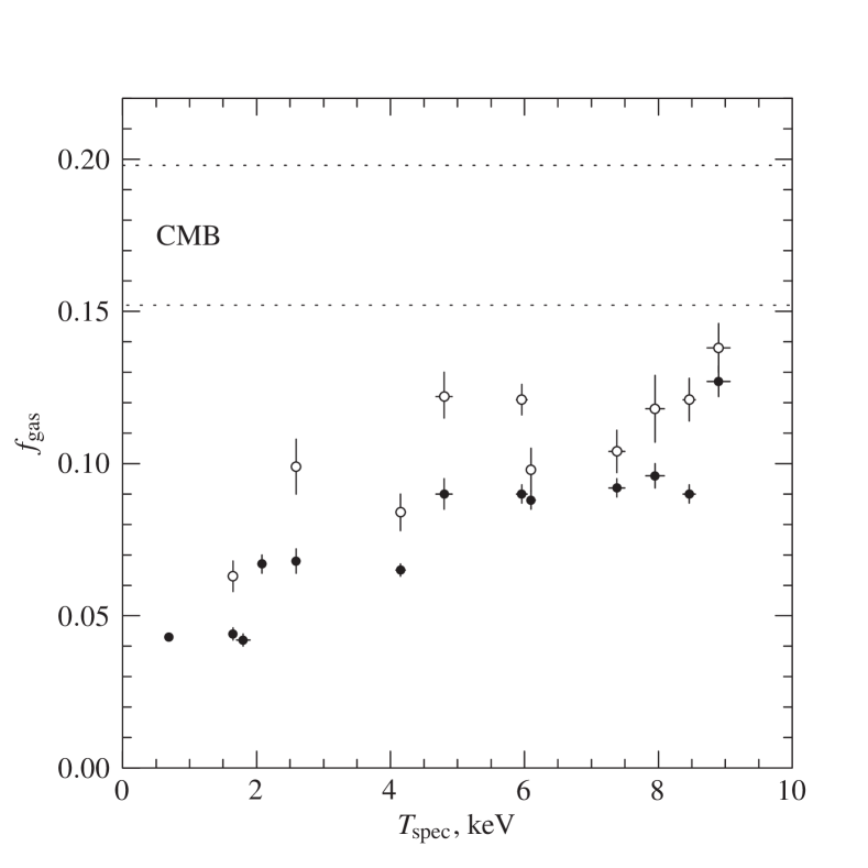
Figure 21.— Observed gas fractions within $r_{2500}$ and $r_{500}$ (solid and open circles, respectively). We do not compute $f_{500}$ for A262, RXJ 1159+5531, and USGC S152 because this requires large extrapolations of the mass model. The $f_{2500}$ value for A2390 ($T=8.9$ keV), can be biased (§ 4).

Note, however, that typically, 40–50% of the total mass within $r_{500}$ is contained within the region $r<r_{2500}$ affected by stellar contribution and non-gravitational heating by AGNs. One can hope that a greater uniformity is observed if this central region is removed entirely from the calculation of $f_{\text{gas}}$. In Fig.22, we plot gas fractions measured in the $r_{2500}$–$r_{500}$ shell. The gas fractions in the shell increase still further relative to $f_{500}$. In fact, they become consistent (albeit within larger uncertainties) with an average of $f_{\text{gas}}\simeq 0.13$ for all clusters, except for the lowest-temperature object (MKW 4). A reasonable correction for the stellar contribution, 10–15% of the ICM mass (e.g., Lin, Mohr & Stanford, 2003; Sanderson & Ponman, 2003; Voevodkin & Vikhlinin, 2004), should then bring the gas fractions within the shell $r_{2500}$–$r_{500}$ into agreement with the Universal value determined from CMB studies.

To summarize, the observed gas fraction shows smaller variations between individual objects, and is closer to the Universal value, when determined at larger radii. This is in line with the general tendency for our clusters to become more self-similar at large radii, as manifested by the 3-dimensional temperature and density profiles, and the $M-T$ relation. The regularity of $f_{\text{gas}}$ determined in the shell $r_{2500}$–$r_{500}$ gives hope that these measurements can be used to determine $\Omega_{m}$ using the classical baryon fraction test (White et al., 1993b). We defer application of this test to a future work because this involves small but important corrections, such as stellar contribution, baryon depletion, accuracy of hydrostatic assumption etc., which are beyond the scope of this paper.

We finally mention that gas fractions within $r_{2500}$ derived from Chandra observations of relaxed clusters were recently used for cosmological constraints in a series of papers by Allen et al. (2004, and references therein). There are significant differences in the $f_{2500}$ derived in our analysis and those reported by Allen et al., as outlined in Appendix B.

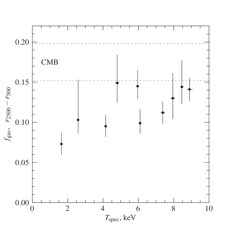
Figure 22.— Observed gas fractions within the shell $r_{2500}$–$r_{500}$. We do not compute $f_{\text{gas}}$ for A262, RXJ 1159+5531, and USGC S152 because this requires large extrapolations of the mass model.

9. Summary and future work

We presented total mass and gas profiles of low-redshift, relaxed clusters using the best available observations with Chandra. The cluster sample (13 objects) spans a range of temperatures of 0.7–9 keV and masses $M_{500}=(0.5-10)\times 10^{14}\,M_{\odot}$. The total masses are derived assuming hydrostatic equilibrium of the ICM in the cluster potential. Our modeling method makes few additional assumptions and allows us to reconstruct the cluster properties relatively model-independently, thus avoiding biases and producing realistic uncertainties on the derived quantities. The main results are summarized below.

1. The shape of the total density profiles in our clusters and their scaling with mass are in good agreement with predictions of $\Lambda$CDM model. They approximately follow the universal density profile with the concentration expected for CDM-dominated halos in this cosmology. The gas density and temperature profiles at large radii are also nearly self-similar, although in the inner region (within $\approx 0.1~{}r_{500}$) there is significant scatter and systematic trend with cluster mass.

2. Correspondingly, we find that the slope of the mass-temperature relation is in good agreement with the simple self-similar behavior, $M_{500}\propto T$ where $\alpha=(1.5-1.6)\pm 0.1$, if the average temperature is measured at radii not affected by the central cool core. We derive an accurate normalization of the $M-T$ relation for relaxed clusters. Our normalization is $\approx 30\%$ higher than most previous X-ray determinations.

3. The gas density profiles are generally not described by a $\beta$-model or its common modifications, even at large radii. The profiles steepen continuously and this behavior can be approximated as a smooth break in the power law index around $(0.5-0.7)\,r_{500}$. Near $r_{500}$, the effective slope of the gas density profile, $-\frac{1}{3}\,d\log\rho_{g}/d\log r\simeq 0.78$, with no detectable dependence on cluster mass.

This behavior of the gas density at large radii is missed by $\beta$-model fits because they are primarily sensitive to the data in the bright inner region. Insufficiently accurate modeling of the gas distribution at large radii, in addition to using polytropic approximations to $T(r)$, explains the lower normalizations of the $M-T$ relation derived in previous studies.

4. We present accurate measurements of the gas mass fraction as a function of radius. We observe strong systematic variations of $f_{\text{gas}}$ both with radius and with cluster mass. The gas fractions within $r_{2500}$ are significantly lower than the Universal baryon fraction suggested by the CMB observations. However, the trends become weaker and the absolute values of $f_{\text{gas}}$ are closer to the Universal value at $r>r_{2500}$.

In future work, we will use these accurate measurements of the gas fractions to constrain $\Omega_{m}$. This requires the inclusion of small but important effects, such as stellar mass, baryon depletion, and correction for biases in the mass measurements, which are beyond of the scope of this paper. We will also present a detailed comparison of the Chandra results on the cluster mass, temperature, and $f_{\text{gas}}$ profiles with high-resolution cosmological simulations.

Appendix A Comparison with previous determinations of the $M-T$ relation

The main differences of our analysis with the previous work on cluster masses is in the more accurate measurements of the gas temperature and density gradients at large radii. Comparison between different studies is facilitated by formulation of the the hydrostatic equlibrium equation ([7]) using effective slopes of the density and temperature profiles.

Let us define the effective bas density slope as $\beta_{\text{eff}}=-\frac{1}{3}\,d\log\rho/d\log r$; for the $\beta$-model, $\beta_{\text{eff}}=\beta\,(r/r_{c})^{2}/(1+(r/r_{c})^{2})\rightarrow\beta$ at large radii. The equivalent quantity for the temperature profile is $\beta_{t}=-1/3\,d\log T/d\log r$. For polytropic parameterization of the temperature profile, $\beta_{\text{eff}}$ and $\beta_{t}$ are related via

$$\frac{d\log T}{d\log r}=(\gamma-1)\frac{d\log T}{d\log r}\quad\text{or}\quad\beta_{t}=(\gamma-1)\,\beta{{}_{\text{eff}}}$$ (A1)

The hydrostatic equilibrium equation [7] can now be rewritten as $M(r)\propto r\times T(r)\times(\beta_{\text{eff}}+\beta_{t})$. To compute the overdensity mass, we solve equation of the type $M(r_{\Delta})/r_{\Delta}^{3}=C$, or $r_{\Delta}^{-2}\,T(r)\,(\beta_{\text{eff}}+\beta_{t})=C$. Therefore, the overdensity mass estimate scales as

$$M_{\Delta}\propto T_{0}^{3/2}\,(T(r)/T_{0})^{3/2}(\beta_{\text{eff}}+\beta_{t})^{3/2},$$ (A2)

where $T_{0}$ is an average temperature, and normalization of the $M-T$ relation scales as

$$A=M_{\Delta}/T_{0}^{3/2}\propto(T(r)/T_{0})^{3/2}(\beta_{\text{eff}}+\beta_{t})^{3/2}$$ (A3)

The quantities $\beta_{\text{eff}}$ and $\beta_{t}$ derived for our clusters at $r_{500}$ are shown in Fig.23.

A.1. ASCA Measurements by Nevalainen et al. and Finoguenov et al.

Nevalainen et al. (2000) and Finoguenov et al. (2001) use ASCA temperature profiles which agree with our Chandra measurements. However, their normalizations for the $M_{500}-T$ relation for $T=5$ keV clusters are lower — $2.2\times 10^{14}\,h^{-1}\,M_{\odot}$ and $2.3\times 10^{14}\,h^{-1}\,M_{\odot}$ in Nevalainen et al. and Finoguenov et al., respectively, compared with our value of $2.93\times 10^{14}\,h^{-1}\,M_{\odot}$ (Table 4, for $T_{\text{spec}}$). There are subtle differences between these studies in how the average temperatures are defined and how the measurements are scaled to $z=0$. The most significant effect, however, is steepening of the gas density profile at large radii that is clearly present in high-quality Chandra data and was hard to detect with earlier X-ray telescopes. This steepening was effectively missed by Nevalainen et al. and Finoguenov et al. because they used pure $\beta$-model fits determined mainly by the data in the inner regions. Indeed, the average $\beta_{\text{eff}}$ at $r_{500}$ is $0.78$ for our clusters (Fig. 23), while it is $\approx 0.65$ for $T>3$ keV clusters in Finoguenov et al. (see their Fig. 5). The average $\beta_{t}$ for our clusters is 0.17, while the Finoguenov et al. value is 0.11 from their average polytropic index of $\gamma\approx 1.17$ for hot clusters (see eq. [A1]). These differences in the slopes should lead (eq. [A2]) to a mismatch in mass estimates by a factor of $(0.78+0.15)^{3/2}/(0.65+0.11)^{3/2}\simeq 1.35$, explaining the offset between our $M-T$ normalizations. We note here that undetected steepening of the gas density profiles at large radii was suggested by Borgani et al. (2004) as a possible reason for low normalization of the Finoguenov et al. $M-T$ relation.

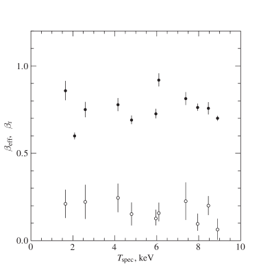
Figure 23.— Effective slopes of gas density and temperature profiles at $r_{500}$

We find no detectable trends in either $\beta_{\text{eff}}$ or $\beta_{t}$ with cluster temperature (Fig. 23). The gas density profiles of cool clusters are indeed flatter in the inner region but they steepen significantly at $r\sim 0.5\,r_{500}$ (Fig. 17). This absence of trends in $\beta_{\text{eff}}$ and $\beta_{t}$ is in fact the main reason why our slopes of mass-temperature relation are close to $1.5$ (cf. eq. [A2]). In contrast, earlier studies based on $\beta$-model fits to the X-ray brightness profiles consistently found very flat density slopes for 1–2 keV clusters. For example, the average $\beta_{\text{eff}}$ for such clusters is $\simeq 0.5$ in Finoguenov et al., while for $T\sim 10$ keV clusters, they find $\beta_{\text{eff}}\approx 0.7$. It follows from eq. [A2] that such a trend in $\beta_{\text{eff}}$ should steepen the slope of the $M-T$ relation from $\alpha=1.5$ to $\alpha\sim 1.72$.

A.2. XMM-Newton Measurements of Arnaud et al.

Our normalization of the $M-T$ relation is very close to that derived by Arnaud et al. (2005) using XMM-Newton data. Given the systematic difference in the temperature profiles at large radii between our two studies (see the discussion in § 5), this is not expected and merits a clarification. In the Arnaud et al. works, temperature profiles are generally interpreted to be consistent with constant at large radii (Pointecouteau et al., 2005). Therefore, the quantities to use in eqs. (A2-A3), $\beta_{t}\simeq 0$ and $T(r)/T_{0}\simeq 1$ near $r_{500}$ for the XMM-Newton masses. E. Pointecouteau and M. Arnaud kindly provided the average gas density slope for their sample, $\langle\beta_{\text{eff}}\rangle=0.71$, only slightly below our value. For our sample, the relevant quantities at $r_{500}$ are $\langle\beta_{\text{eff}}\rangle=0.78$, $\langle\beta_{t}\rangle=0.17$, and $\langle T(r)/T_{0}\rangle=0.67$, where $T_{0}$ is the spectroscopic average temperature (see § 3.5). From eq. [A3] we would then expect the XMM-Newton $M_{500}-T$ normalization to be a factor of $1.18$ higher than our value, while in fact it is slightly lower (Fig.19).

The reason is that for the $M-T$ relation, Arnaud et al. used cluster masses derived by fitting an NFW model to the data within $\sim r_{1000}$, their maximum radius of observation. This gives systematically lower masses at $r\gtrsim r_{500}$ than the values obtained by direct hydrostatic derivation using extrapolation of the isothermal temperature profiles (E. Pointecouteau & M. Arnaud, private communication). In effect, the masses from the NFW fit imply declining temperature profiles at large radii, such as those observed by Chandra. To summarize, the agreement between our $M-T$ normalizations is somewhat a coincidence.

Note also that the XMM-Newton cluster temperatures are systematically lower than those from Chandra (see e.g., Vikhlinin et al., 2005)), but this does not change the normalization of the $M-T$ relation as it moves the clusters along the relation.

We also used the results from the Pointecouteau et al. (2005) sample to check our mass derivation algorithm. The published XMM-Newton temperature and density profiles were used as input to our procedure. The obtained mass profiles were nearly identical to those from Pointecouteau et al.

Appendix B Comparison with $f_{\text{gas}}$ measurements of Allen et al.

Gas fractions within $r_{2500}$ derived from Chandra observations of relaxed clusters were recently used for cosmological constraints in a series of papers by Allen et al. (2004, and references therein). There are significant differences in the $f_{\text{gas},2500}$ derived in our analysis and in Allen et al., as outlined below.

For all our $T>5$ keV clusters except A2390, we derive lower values of $f_{\text{gas}}$. Our average value for these clusters is $f_{\text{gas}}=0.091\pm 0.002$, compared to an average of $0.117\pm 0.002$ in Allen et al. (same temperature range and same cosmology). The same $\sim 25\%$ difference holds for the four clusters common in both samples, A2029, A478, A1413, and A383 (see Table 2 in Allen et al. 2004 and our Table 3).

We also do not observe flattening of $f_{\text{gas}}(r)$ at radii within $r_{2500}$ as reported, e.g., in Allen, Schmidt & Fabian (2002). Note, however, that a larger sample presented in Allen et al. (2004) shows more variety in the behavior of $f_{\text{gas}}(r)$ profiles.

Profiles for individual clusters in the Allen et al. sample were either not published or published prior to significant Chandra calibration updates. Therefore, we are unable to perform a more detailed object-to-object comparison.

References

- Akritas & Bershady (1996) Akritas, M. G. & Bershady, M. A. 1996, ApJ, 470, 706
- Allen et al. (2001a) Allen, S. W., Ettori, S., & Fabian, A. C. 2001a, MNRAS, 324, 877
- Allen et al. (2004) Allen, S. W., Schmidt, R. W., Ebeling, H., Fabian, A. C., & van Speybroeck, L. 2004, MNRAS, 353, 457
- Allen et al. (2001b) Allen, S. W., Schmidt, R. W., & Fabian, A. C. 2001b, MNRAS, 328, L37
- Allen et al. (2002) Allen, S. W., Schmidt, R. W., & Fabian, A. C. 2002, MNRAS, 334, L11
- Anders & Grevesse (1989) Anders, E. & Grevesse, N. 1989, Geochim. Cosmochim. Acta, 53, 197
- Arabadjis et al. (2004) Arabadjis, J. S., Bautz, M. W., & Arabadjis, G. 2004, ApJ, 617, 303
- Arnaud & Evrard (1999) Arnaud, M. & Evrard, A. E. 1999, MNRAS, 305, 631
- Arnaud et al. (2005) Arnaud, M., Pointecouteau, E., & Pratt, G. W. 2005, A&A, submitted (astro-ph/0502210)
- Bell et al. (2003) Bell, E. F., McIntosh, D. H., Katz, N., & Weinberg, M. D. 2003, ApJS, 149, 289
- Borgani et al. (2004) Borgani, S., et al. 2004, MNRAS, 348, 1078
- Bryan & Norman (1998) Bryan, G. L. & Norman, M. L. 1998, ApJ, 495, 80
- Bullock et al. (2001) Bullock, J. S., Kolatt, T. S., Sigad, Y., Somerville, R. S., Kravtsov, A. V., Klypin, A. A., Primack, J. R., & Dekel, A. 2001, MNRAS, 321, 559
- Buote & Lewis (2004) Buote, D. A. & Lewis, A. D. 2004, ApJ, 604, 116
- Cavaliere & Fusco-Femiano (1978) Cavaliere, A. & Fusco-Femiano, R. 1978, A&A, 70, 677
- David et al. (2001) David, L. P., Nulsen, P. E. J., McNamara, B. R., Forman, W., Jones, C., Ponman, T., Robertson, B., & Wise, M. 2001, ApJ, 557, 546
- De Grandi & Molendi (2002) De Grandi, S. & Molendi, S. 2002, ApJ, 567, 163
- Dolag et al. (2004a) Dolag, K., Bartelmann, M., Perrotta, F., Baccigalupi, C., Moscardini, L., Meneghetti, M., & Tormen, G. 2004a, A&A, 416, 853
- Dolag et al. (2004b) Dolag, K., Jubelgas, M., Springel, V., Borgani, S., & Rasia, E. 2004b, ApJ, 606, L97
- Dubinski & Carlberg (1991) Dubinski, J. & Carlberg, R. G. 1991, ApJ, 378, 496
- Eke et al. (1996) Eke, V. R., Cole, S., & Frenk, C. S. 1996, MNRAS, 282, 263
- Eke et al. (1998) Eke, V. R., Cole, S., Frenk, C. S., & Henry, J. P. 1998, MNRAS, 298, 1145
- Eke et al. (2001) Eke, V. R., Navarro, J. F., & Steinmetz, M. 2001, ApJ, 554, 114
- Ettori (2003) Ettori, S. 2003, MNRAS, 344, L13
- Ettori & Fabian (1999) Ettori, S. & Fabian, A. C. 1999, MNRAS, 305, 834
- Evrard et al. (1996) Evrard, A. E., Metzler, C. A., & Navarro, J. F. 1996, ApJ, 469, 494
- Faltenbacher et al. (2005) Faltenbacher, A., Kravtsov, A. V., Nagai, D., & Gottlöber, S. 2005, MNRAS, 358, 139
- Finoguenov et al. (2001) Finoguenov, A., Reiprich, T. H., & Böhringer, H. 2001, A&A, 368, 749
- Frenk et al. (1990) Frenk, C. S., White, S. D. M., Efstathiou, G., & Davis, M. 1990, ApJ, 351, 10
- Gnedin et al. (2004) Gnedin, O. Y., Kravtsov, A. V., Klypin, A. A., & Nagai, D. 2004, ApJ, 616, 16
- Helsdon & Ponman (2000) Helsdon, S. F. & Ponman, T. J. 2000, MNRAS, 315, 356
- Henry (1997) Henry, J. P. 1997, ApJ, 489, L1
- Henry (2000) Henry, J. P. 2000, ApJ, 534, 565
- Henry & Arnaud (1991) Henry, J. P. & Arnaud, K. A. 1991, ApJ, 372, 410
- Horner et al. (1999) Horner, D. J., Mushotzky, R. F., & Scharf, C. A. 1999, ApJ, 520, 78
- Hu & Kravtsov (2003) Hu, W. & Kravtsov, A. V. 2003, ApJ, 584, 702
- Ikebe et al. (2002) Ikebe, Y., Reiprich, T. H., Böhringer, H., Tanaka, Y., & Kitayama, T. 2002, A&A, 383, 773
- Jenkins et al. (2001) Jenkins, A., Frenk, C. S., White, S. D. M., Colberg, J. M., Cole, S., Evrard, A. E., Couchman, H. M. P., & Yoshida, N. 2001, MNRAS, 321, 372
- Jing (2000) Jing, Y. P. 2000, ApJ, 535, 30
- Kay et al. (2004) Kay, S. T., Thomas, P. A., Jenkins, A., & Pearce, F. R. 2004, MNRAS, 355, 1091
- Kazantzidis et al. (2004) Kazantzidis, S., Kravtsov, A. V., Zentner, A. R., Allgood, B., Nagai, D., & Moore, B. 2004, ApJ, 611, L73
- Kravtsov et al. (2005) Kravtsov, A. V., Nagai, D., & Vikhlinin, A. A. 2005, ApJ, 625, 588
- Lewis et al. (2003) Lewis, A. D., Buote, D. A., & Stocke, J. T. 2003, ApJ, 586, 135
- Lilje (1992) Lilje, P. B. 1992, ApJ, 386, L33
- Lin & Mohr (2004) Lin, Y. & Mohr, J. J. 2004, ApJ, 617, 879
- Lin et al. (2003) Lin, Y., Mohr, J. J., & Stanford, S. A. 2003, ApJ, 591, 749
- Markevitch (1998) Markevitch, M. 1998, ApJ, 504, 27
- Markevitch et al. (1998) Markevitch, M., Forman, W. R., Sarazin, C. L., & Vikhlinin, A. 1998, ApJ, 503, 77
- Markevitch & Vikhlinin (1997) Markevitch, M. & Vikhlinin, A. 1997, ApJ, 491, 467
- Markevitch et al. (1999) Markevitch, M., Vikhlinin, A., Forman, W. R., & Sarazin, C. L. 1999, ApJ, 527, 545
- Mathews (1978) Mathews, W. G. 1978, ApJ, 219, 413
- McNamara et al. (2005) McNamara, B. R., Nulsen, P. E. J., Wise, M. W., Rafferty, D. A., Carilli, C., Sarazin, C. L., & Blanton, E. L. 2005, Nature, 433, 45
- Mohr et al. (1999) Mohr, J. J., Mathiesen, B., & Evrard, A. E. 1999, ApJ, 517, 627
- Motl et al. (2004) Motl, P. M., Burns, J. O., Loken, C., Norman, M. L., & Bryan, G. 2004, ApJ, 606, 635
- Nagai et al. (2003) Nagai, D., Kravtsov, A. V., & Kosowsky, A. 2003, ApJ, 587, 524
- Navarro et al. (1996) Navarro, J. F., Frenk, C. S., & White, S. D. M. 1996, ApJ, 462, 563
- Navarro et al. (1997) Navarro, J. F., Frenk, C. S., & White, S. D. M. 1997, ApJ, 490, 493
- Neumann & Arnaud (1999) Neumann, D. M. & Arnaud, M. 1999, A&A, 348, 711
- Nevalainen et al. (2000) Nevalainen, J., Markevitch, M., & Forman, W. 2000, ApJ, 532, 694
- Nulsen et al. (2005) Nulsen, P. E. J., Hambrick, D. C., McNamara, B. R., Rafferty, D., Birzan, L., Wise, M. W., & David, L. P. 2005, ApJ, 625, L9
- Oukbir & Blanchard (1992) Oukbir, J. & Blanchard, A. 1992, A&A, 262, L21
- Pointecouteau et al. (2004) Pointecouteau, E., Arnaud, M., Kaastra, J., & de Plaa, J. 2004, A&A, 423, 33
- Pointecouteau et al. (2005) Pointecouteau, E., Arnaud, M., & Pratt, G. W. 2005, A&A, 435, 1
- Pratt & Arnaud (2002) Pratt, G. W. & Arnaud, M. 2002, A&A, 394, 375
- Press et al. (1992) Press, W. H., Teukolsky, S. A., Vettering, W. T., & Flannery, B. P., Numerical Recipes (Cambridge: Cambridge Univ. Press, 1992)
- Randall et al. (2002) Randall, S. W., Sarazin, C. L., & Ricker, P. M. 2002, ApJ, 577, 579
- Rasia et al. (2005) Rasia, E., Mazzotta, P., Borgani, S., Moscardini, L., Dolag, K., Tormen, G., Diaferio, A., & Murante, G. 2005, ApJ, 618, L1
- Rasia et al. (2004) Rasia, E., Tormen, G., & Moscardini, L. 2004, MNRAS, 351, 237
- Readhead et al. (2004) Readhead, A. C. S., et al. 2004, Science, 306, 836
- Rines et al. (1999) Rines, K., Forman, W., Pen, U., Jones, C., & Burg, R. 1999, ApJ, 517, 70
- Sanderson & Ponman (2003) Sanderson, A. J. R. & Ponman, T. J. 2003, MNRAS, 345, 1241
- Sanderson et al. (2003) Sanderson, A. J. R., Ponman, T. J., Finoguenov, A., Lloyd-Davies, E. J., & Markevitch, M. 2003, MNRAS, 340, 989
- Sarazin (1988) Sarazin, C. L., X-ray Emission from Clusters of Galaxies (Cambridge: Cambridge University Press, 1988)
- Sheth & Tormen (1999) Sheth, R. K. & Tormen, G. 1999, MNRAS, 308, 119
- Snowden et al. (1994) Snowden, S. L., McCammon, D., Burrows, D. N., & Mendenhall, J. A. 1994, ApJ, 424, 714
- Spergel et al. (2003) Spergel, D. N., et al. 2003, ApJS, 148, 175
- Sunyaev & Zeldovich (1972) Sunyaev, R. A. & Zeldovich, Y. B. 1972, Comments on Astrophysics and Space Physics, 4, 173
- Tasitsiomi et al. (2004) Tasitsiomi, A., Kravtsov, A. V., Gottlöber, S., & Klypin, A. A. 2004, ApJ, 607, 125
- Vikhlinin (2005) Vikhlinin, A. 2005, ApJ submitted (astro-ph/0504098)
- Vikhlinin et al. (1999) Vikhlinin, A., Forman, W., & Jones, C. 1999, ApJ, 525, 47
- Vikhlinin et al. (2005) Vikhlinin, A., Markevitch, M., Murray, S. S., Jones, C., Forman, W., & Van Speybroeck, L. 2005, ApJ, in press, astro-ph/0412306 (Paper I)
- Vikhlinin et al. (1998) Vikhlinin, A., McNamara, B. R., Forman, W., Jones, C., Quintana, H., & Hornstrup, A. 1998, ApJ, 502, 558
- Voevodkin & Vikhlinin (2004) Voevodkin, A. & Vikhlinin, A. 2004, ApJ, 601, 610
- Voit (2005) Voit, G. M. 2005, Reviews of Modern Physics, 77, 207
- Wechsler et al. (2002) Wechsler, R. H., Bullock, J. S., Primack, J. R., Kravtsov, A. V., & Dekel, A. 2002, ApJ, 568, 52
- White (2001) White, M. 2001, A&A, 367, 27
- White et al. (1993a) White, S. D. M., Efstathiou, G., & Frenk, C. S. 1993a, MNRAS, 262, 1023
- White et al. (1993b) White, S. D. M., Navarro, J. F., Evrard, A. E., & Frenk, C. S. 1993b, Nature, 366, 429
- Xu et al. (2001) Xu, H., Jin, G., & Wu, X. 2001, ApJ, 553, 78