Chandra Observations of Shock Kinematics in Supernova Remnant 1987A

Abstract

We report the first results from deep X-ray observations of the SNR 1987A with the Chandra LETG. Temperatures inferred from line ratios range from $\sim 0.1-2$ keV and increase with ionization potential. Expansion velocities inferred from X-ray line profiles range from $\sim 300-1700$  km s^-1 , much less than the velocities inferred from the radial expansion of the radio and X-ray images. We can account for these observations with a scenario in which the X-rays are emitted by shocks produced where the supernova blast wave strikes dense protrusions of the inner circumstellar ring, which are also responsible for the optical hot spots.

1 Introduction

With the rapidly developing impact of the debris of Supernova 1987A with its inner circumstellar ring, we have an unprecedented opportunity to witness the birth of a supernova remnant, SNR1987A (McCray 2005). This event, the first hint of which was the 1995 appearance of Spot 1, a rapidly brightening optical ‘hotspot’ on the ring, has now evolved to the stage that the ring is encircled by hotspots (Sugerman et al. 2002). Additionally, an annular source of X-ray emission correlated with the locations of the hotspots has brightened at an accelerating rate (Park et al. 2004). Evidently, the optical hotspots appear where the supernova blast wave encounters fingers of relatively dense gas protruding inwards from the ring. In such a situation, a complex hydrodynamic interaction ensues (cf. Borkowski, Blondin & McCray 1997a,b). The optical emission from the spots comes from relatively slow ($V_{S}\leq 200$ km s^-1) shocks which have had time to undergo radiative cooling (Pun et al. 2002). The X-ray emission must come from gas heated by faster ($V_{S}\geq 1000$ km s^-1) shocks, either transmitted shocks entering the protrusions or shocks reflected from the protrusions.

Michael et al. (2002) reported the first observation of a dispersed X-ray spectrum of SNR 1987A, taken in October 1999 with HETG on the Chandra observatory. The X-ray emission was dominated by shock-heated gas having electron temperature $kT_{e}\approx 2.6$ keV. Due to the poor photon statistics, only a composite line profile was constructed by stacking the profiles of the individual observed lines. From the measured FWHM ($\approx 5000$ km s^-1), they inferred that the X-ray emitting gas was moving with radial velocity $\approx 3500$ km s^-1, roughly the same as that inferred from the observed proper motion of the non-thermal radio source (Manchester et al. 2002) and the X-ray source (Park et al. 2004).

From October 1999 to September 2004, the X-ray source SNR1987A has brightened by a factor $\sim 10$ (Park et al. 2005). As a result, it has become possible with Chandra to obtain dispersed X-ray spectra with very high counting statistics. In this Letter, we report the first results from the analysis of such observations.

2 Observations and Data Reduction

SNR 1987A was observed with Chandra in the configuration LETG-ACIS-S in five consecutive runs during Aug 26 – Sep 5, 2004, providing a total effective exposure of 289 ksec. We extracted positive and negative first-order LETG spectra for each of the five observations. Then, we merged the resultant spectra into one spectrum each for the positive and negative LETG arms with respective total counts of 9,241 and 6,057 in the energy range 0.4 - 7 keV. The difference in photon statistics is a result of the different sensitivities of the respective CCD detectors. We also extracted the pulse-height spectrum from the zeroth-order image with a total number of 16,557 counts in the 0.4 - 7 keV range. Figure 1 demonstrates the enormous scientific advantage of the dispersed spectrum over the pulse-height spectrum.

We fitted the strong emission line triplets of various He-like ions by a sum of three Gaussians and constant local continuum. The ratio of line centers of the triplet components were held fixed according to the values given by the Chandra atomic database¹ and all components shared the same full width at half maximum (FWHM). Thus, free parameters were the intensities of their components, the line center wavelength of one of the components, FWHM, and the local continuum. Likewise, we fitted the strong emission doublets of the H-like species but the component intensities were fixed through their atomic data values. We found that the centroid shifts for the strong emission lines were consistent with the red-shift of the Large Magellanic Cloud, and that the line fluxes derived from the positive and negative first-order spectra agreed within expected statistical uncertainties. Therefore, we assumed that all the line centers had the same Doppler shift, $V_{D}=286$ km s^-1 , and fitted the positive and negative first-order spectra simultaneously.

3 Line Fluxes and Ratios

Table 1 lists the fluxes of all the emission lines and multiplets that could be measured with acceptable photon statistics. Given the excellent spectral resolution and photon statistics, we can for the first time derive reliable intensities and ratios of various X-ray emission lines from SNR 1987A. As we shall discuss in § 5, we expect the actual conditions in the plasma to be sufficiently complex that we can only use the line strengths and ratios to infer typical conditions of the plasma responsible for the emission by a given ion. The ratio of He-like(K_α)/H-like(Ly_α) from a given element is sensitive to both temperature and ionization state of the gas. The same is true for the ‘G-ratio’ of the He-like triplet lines ($G=\frac{f+i}{r}$ where ‘f’, ‘i’ and ‘r’ stand for forbidden, intercombination and recombination lines, respectively) since these lines are produced not only by electron impact excitation of the He-like ions but also by K-shell ionization of the Li-like ions (Mewe 1999; Liedahl 1999).

Since we expect that shocks are responsible for heating and ionizing the X-ray emitting gas, we can compare our measured line ratios to those resulting from the XSPEC code, which provides models of the time-dependent ionization and X-ray emission from plane-parallel shocks (Borkowski, Lyerly, & Reynolds 2001). In such models, the line ratios are functions of the post-shock temperature and the ionization age, $n_{e}t$, defined as the time since the gas first entered the shock times the postshock electron density. The X-ray emitting plasma in SNR 1987A is in NEI (nonequilibrium ionization), and so inner-shell ionization and excitation contribute importantly to emission line ratios. Indeed, if these processes are not included, the theoretical G-ratios cannot match the observed ones.

In Figure 2, the curves define those regions in the parameter space of electron temperature and ionization age, $n_{e}t$, for which the observed line ratios agree with the ratios that would result from a plane parallel shock. Except for a very narrow range of $n_{e}t$, the inferred temperatures are likely to be in the range 0.1–2 keV. We see immediately that no single combination of electron temperature and ionization age is consistent with all the observed ratios. Instead, for any given ionization age, the inferred electron temperature increases tentatively with ionization potential. Evidently, the X-ray emission comes from a distribution of shocks having a range of ionization ages and post-shock temperatures.

4 Line Profiles

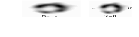
Figure 3: A schematic view of the LETG observational situation for SNR 1987A using the deconvolved zeroth-order total image. The X-ray source is assumed to be an inclined ring, the northern (N) side of which is blue-shifted and the southern (S) side of which is red-shifted. Shown are the zeroth-order image ($m=0$), as well as the positive ($m=+1$) and negative ($m=-1$) images in an arbitrary spectral line. The dispersion direction is horizontal.

The excellent spatial and spectral resolution of Chandra allows us for the first time to observe the kinematics of the X-ray emitting gas through the line profiles. The method is illustrated by Figure 3. We assume that the X-ray source lies on a circular ring having angular radius $\theta_{R}$ and that this ring is expanding with constant radial velocity, $V_{R}$. We also assume that the X-ray source has, like the optical inner circumstellar ring, inclination angle $i=44-45^{\circ}$, with the near side to the north and minor axis at P.A. $\approx 354^{\circ}$  (Sugerman et al. 2002). The roll angle was chosen so that the negative ($m=-1$) arm of the dispersion axis was aligned at P.A. $\approx 345^{\circ}$, thus, the north side of the ring will be blue-shifted and the south side will be red-shifted. The dispersed images of the ring will be distorted by these Doppler shifts.² In the $m=-1$ image, the N side of the ring will be displaced to the left, and the S side will be displaced toward the right. Thus, the minor axis of the $m=-1$ image will be compressed. Likewise, the minor axis of the $m=+1$ image will be stretched.

This behavior is exactly what we see in the measured line profiles. We fitted Gaussian profiles (as explained in § 2) to each emission line or multiplet independently in the $m=+1$ and $m=-1$ first-order spectra. In every case, the width of a given emission line in the $m=+1$ arm is greater than the corresponding width in the $m=-1$ arm (Fig. 1). The actual line profile will likely differ from a Gaussian due to the complex spatial-spectral effects. However, the Gaussian approximation is sufficient for the analysis presented here (resulting in a reduced $\chi^{2}\approx 1$ for each of the line-profile fits).

There are two major sources of line broadening in the dispersed images. One is the spatial extent of the image itself, which can be expressed as an equivalent line broadening, independent of wavelength. The second is the broadening due to the bulk motion of the shocked gas. We express the net line width (FWHM) broadening as:

$$\Delta\lambda_{tot}=2\Delta\lambda_{0}\pm 2z_{0}(\lambda/\lambda_{0})^{\alpha}\lambda\,,~{}$$ (1)

where the plus (minus) sign refers to the $m=+1$ ($m=-1$) spectrum, respectively. The two sources of broadening are represented respectively by the first and second term on the right hand side of equation (1). The power-law function of wavelength allows for the possibility that the mean bulk velocity of shocked gas emitting a given line may depend on the excitation or ionization stage of the emitting ion. The parameter $z_{0}$ determines the line broadening at some fiducial wavelength, $\lambda_{0}$, and the power-law index $\alpha$ is to be determined.

We then fit equation (1) to the data in Figure 1. We consider two models. In the first (constant velocity) model, we assume that all emitting ions have the same mean bulk velocity ($\alpha=0$). In that case, we find a best-fit value $z_{0}=0.0006$. In the second (stratified) model, we allow the values of $\alpha$ and $z_{0}$ to vary. In that case, we find a best-fit value $\alpha=-1.3$. Note that such a negative value of $\alpha$ implies that emission lines with shorter wavelength are produced by gas having greater radial velocity, as expected. The stratified model provides a slightly better fit to the data than the constant velocity model ($\chi^{2}/dof=22/19$ vs. $25/20$), but the data are not good enough to distinguish between the models with confidence. We may translate the fitting parameters into an equivalent mean radial bulk velocity, $V_{r}$, of an expanding circular ring by adopting an average value for the azimuthal $\phi$ ($\overline{\sin\phi}=2/\pi~{},0\leq\phi\leq\pi/2$) and a value ($i=45^{\circ}$) for the inclination of the inner ring. This yields a value $V_{r}=397$ km s^-1. In the case of a strong radial shock with adiabatic index $\gamma=5/3$, the corresponding shock velocity must be $V_{S}=4V_{r}/3=530$ km s^-1 . The corresponding shock velocity in the stratified case is given by $V_{S}(\lambda)=920~{}(\lambda/10$Å)^-1.3 km s^-1 . Finally, we note that in the both models the derived source half-size of $\Delta\lambda_{0}=0.047$ Å  or $\theta_{R}=0\farcs 84$ is consistent with the SNR 1987A size from an X-ray image-deconvolution technique (Burrows et al. 2000). Thus, we are confident that the simplified treatment presented here gives reliable results.

5 Discussion and Conclusions

The most surprising result of this observation is the relatively low velocity of the X-ray emitting gas as determined from the line profiles. When we proposed to do this observation, we expected to see kinematic velocities in the range $\sim 2500-3000$ km s^-1 , as we saw in the composite line profile measured with the Chandra HETG in October 1999 (Michael et al. 2002) and in the radial expansion rate of the X-ray image (Park et al 2004). At the very least, we would expect to see velocities comparable to the velocity of gas behind a shock moving sufficiently fast to heat the electrons to temperatures inferred from the X-ray line ratios. For a shock of high Mach number entering stationary gas with velocity $V_{S}$, the maximum electron temperature is: $kT_{e}=\frac{3}{16}\mu V_{S}^{2}=1.4(V_{S}/1000~{}\mathrm{km~{}s^{-1}})^{2}\hskip 14.22636pt$ keV. The value $V_{S}=530$ km s^-1 inferred for the constant velocity model then implies a post-shock temperature $kT_{e}\leq 0.39$ keV. This value is inconsistent with the temperatures required to account for the $K_{\alpha}/L_{\alpha}$ line ratios observed for Mg and Si (Fig. 2). On the other hand, the electron temperatures inferred from the line profiles in the stratified model may be consistent with the observed line ratios ($kT_{e}=0.15-4.0$ keV for $V_{S}=340-1,700$ km s^-1 ).

How do we reconcile the relatively low gas velocities inferred from the line profiles with the much greater velocities inferred from the radial expansion rate of the X-ray image? We have in mind a picture in which a blast wave of velocity $V_{B}\sim 3000$ km s^-1 propagates through the low atomic density ($n_{0}\sim 100$ cm^-3) gas inside the circumstellar ring. A zone of enhanced X-ray emission appears when the blast wave strikes a finger of relatively dense ($n_{1}\sim 3\times 10^{3}-3\times 10^{4}$ cm^-3) gas protruding inward from the ring. A transmitted shock propagates into the protrusion at velocity reduced by a factor $\sim(n_{1}/n_{0})^{1/2}$, while a reflected shock propagates backwards. The latter increases the density and temperature of the circumstellar matter to values substantially greater than those caused by the original blast wave, and it also reduces the radial velocity of the doubly-shocked circumstellar gas. The enhanced X-ray emission comes from the gas behind the transmitted shock and from the gas behind the reflected shock, with the proportional contributions depending on the details of the hydrodynamics. But, the lower velocity of the transmitted shock and the high density behind it ensure a short cooling timescale and eventually increased optical emission. At each point of impact with a protrusion, a new zone of enhanced X-ray emission appears. Thus, the mean radius of the enhanced X-ray emission appears to move outward at a substantial fraction of the blast wave velocity, while the gas responsible for most of the X-ray emission may be moving much more slowly. This picture assumes that only a small fraction of the blast wave area is covered by protrusions at the present time. It also implies that the radial expansion of the X-ray image should slow down rapidly as the blast wave overtakes the entire equatorial ring.

The scenario that we have described here accounts in a natural way for several properties observed by Chandra images and spectra of SNR 1987A: (1) the correlation of the rapid X-ray brightening with the appearance of the optical hotspots; (2) the correlation of the X-ray image with the optical hotspots; (3) the relatively rapid expansion of the X-ray image compared to the relatively slow bulk velocity of the X-ray-emitting gas; and (4) the correlation of the inferred electron temperature and expansion velocity of the shocked gas with excitation potential of X-ray emission lines.

There is much more to be learned from the Chandra spectroscopic data beyond the brief summary that we have presented here. By fitting global models for the entire X-ray spectrum, we can infer element abundances and the distribution of emission measure with temperature. By simulating the actual 2-dimensional images in the dispersed spectra (e.g., with the MARX software), we can refine our models of the kinematics and spatial distribution of the shocked gas. By constructing simulations of the hydrodynamics of the impact of the blast wave with the protrusions, we hope to provide a more refined interpretation of the observations than the analysis presented here.

Figure 1: Left panel: The background-subtracted LETG first ($+1$, solid) and zeroth-order (dashed) spectra. Right panel: Measured line widths (FWHM) for the positive (diamonds) and negative (squares) LETG arms, respectively. The solid curve represents the resolving power of the LETG ($E/\Delta~{}E\approx 20\lambda$). The dashed and dotted curves correspond to the line broadening parameter in the cases with and without shock stratification (see § 4).

Figure 2: Isolines of the G-ratios (dots) and the K_α/L_α ratios (dashes) for O, Ne, Mg and Si. Note that the G-ratios include the line contribution from inner-shell processes (see text). The three curves for each ratio correspond to the measured value and $\pm 1\sigma$. The K_α/L_α ratios have been corrected for differential X-ray absorption assuming N${}_{H}=1.6\times 10^{21}$ cm^-2. The observed G-ratios are: $1.44\pm 0.47$ (O); $0.87\pm 0.11$ (Ne); $0.79\pm 0.09$ (Mg); $1.17\pm 0.23$ (Si).

Table 1: SNR 1987A: Line Fluxes

Line	IPa	$\lambda_{lab}$b	Flux c	Counts d
S XV Kα	3.22	5.0387	5.14 $\pm$ 2.15	87.5 $\pm$ 36.6
Si XIV Lα	2.67	6.1804	2.22 $\pm$ 0.46	102.7 $\pm$ 21.3
Si XIII Kα	2.44	6.6479	11.86 $\pm$ 1.19	522.7 $\pm$ 52.4
Mg XII Lα	1.96	8.4192	7.33 $\pm$ 0.96	250.6 $\pm$ 32.8
Mg XI Kα	1.76	9.1687	18.09 $\pm$ 1.11	475.7 $\pm$ 29.2
Ne X Lα	1.36	12.1321	36.40 $\pm$ 2.40	552.3 $\pm$ 36.4
Ne IX Kα	1.20	13.4473	60.68 $\pm$ 3.82	838.2 $\pm$ 52.8
Fe XVIIe	1.27	15.0140	38.10 $\pm$ 3.20	450.4 $\pm$ 37.7
O VIII Lβ	0.87	16.0055	19.90 $\pm$ 2.40	204.7 $\pm$ 24.7
Fe XVIIe	1.27	16.7800	24.14 $\pm$ 3.18	336.4 $\pm$ 37.8
O VIII Lα	0.87	18.9671	50.80 $\pm$ 4.00	377.3 $\pm$ 29.7
O VII Kα	0.74	21.6015	35.20 $\pm$ 5.77	162.8 $\pm$ 26.7
N VII Lα	0.67	24.7792	44.90 $\pm$ 5.20	203.7 $\pm$ 23.6

References

- A (1) Borkowski, K.J., Blondin, J.M., & McCray, R. 1997a, ApJ, 476, L31
- A (2) Borkowski, K.J., Blondin, J.M., & McCray, R. 1997b, ApJ, 477, 281
- A (3) Borkowski, K.J., Lyerly, W.J., & Reynolds, S.P., 2001, ApJ, 548, 820
- A (5) Burrows, D.N. et al. 2000, ApJ, 543, L149
- A (7) Liedahl, D.A. 1999, in X-ray Spectroscopy in Astrophysics, eds. J. van Paradijs and J.A.M. Bleeker, Lecture Notes in Physics, 520, 189
- A (8) Manchester, R.N., Gaensler, B.M., Wheaton, V.C., Staveley-Smith, L., Tzioumis, A.K., Bizunok, N.S., Kesteven, M.J., & Reynolds, J.E. 2002, PASA, 19, 207
- (7) McCray, R. 2005, in Cosmic Explosions, IAU Colloquium #192, eds. J. M. Marcaide and K. W. Weiler (Heidelberg: Springer Verlag), 77
- A (9) Mewe, R. 1999, in X-ray Spectroscopy in Astrophysics, eds. J. van Paradijs and J.A.M. Bleeker, Lecture Notes in Physics, 520, 109
- A (10) Michael, E. et al. 2002, ApJ, 574, 166
- (10) Park, S., Zhekov, S. A., Burrows, D. N., Garmire, G. P., & McCray, R. 2004, ApJ, 610, 275
- (11) Park, S., Zhekov, S. A., Burrows, D. N., Garmire, G. P., & McCray, R. 2005, Adv. Sp. Res. , in press (astro-ph/0501561)
- A (12) Pun, C.S.J. et al. 2002, ApJ, 572, 906
- A (15) Sugerman, B.E.K., Lawrence, S.S., Crotts, A.P.S., Bouchet, P., & Heathcote, S.R. 2002, ApJ, 572, 209