A Search for Untriggered GRB Afterglows with ROTSE-III

Abstract

We present the results of a search for untriggered gamma-ray burst (GRB) afterglows with the Robotic Optical Transient Search Experiment-III (ROTSE-III) telescope array. This search covers observations from September 2003 to March 2005. We have an effective coverage of $1.74\,\mathrm{deg}^{2}\,\mathrm{yr}$ for rapidly fading transients that remain brighter than $\sim 17.5$ magnitude for more than 30 minutes. This search is the first large area survey to be able to detect typical untriggered GRB afterglows. Our background rate is very low and purely astrophysical. We have found 4 previously unknown cataclysmic variables (CVs) and 1 new flare star. We have not detected any candidate afterglow events or other unidentified transients. We can place an upper limit on the rate of fading optical transients with quiescent counterparts dimmer than $\sim\,20^{th}$ magnitude at a rate of less than $1.9\,\mathrm{deg}^{-2}\,\mathrm{yr}^{-1}$ with 95% confidence. This places limits on the optical characteristics of off-axis (orphan) GRB afterglows. As a byproduct of this search, we have an effective $\sim 52\,\mathrm{deg}^{2}\,\mathrm{yr}$ of coverage for very slowly decaying transients, such as CVs. This implies an overall rate of outbursts from high galactic latitude CVs of $0.1\,\mathrm{deg}^{-2}\,\mathrm{yr}^{-1}$.

1. Introduction

There is much circumstantial evidence that gamma-ray burst (GRB) outflows are highly relativistic and collimated. An achromatic break has been seen in light curves for several GRB afterglows, with the canonical example being GRB 990510. (Harrison et al., 1999; Stanek et al., 1999) These breaks are naturally explained by a geometric constraint on the outflow. The jet opening angle has been inferred for GRB 990510 and several other GRBs, and appears to range from $2^{\circ}$ to $30^{\circ}$. (Frail et al., 2001; Panaitescu & Kumar, 2001) Therefore, the true rate of GRBs must be $\gtrsim 100$ times that detected by satellite experiments such as BATSE, HETE-2, INTEGRAL, and Swift. Although the Earth will not receive $\gamma$-ray emission from these bursts, they might be detectable at longer wavelengths. It remains an open question what these off-axis “orphan” afterglows should look like. In the simplest model, an orphan afterglow looks like a standard afterglow, except that it becomes visible after a delay of $\sim 0.5\,\mathrm{day}$. As the ejecta cools, the relativistic beaming angle increases until the afterglow can be seen off-axis, long after the $\gamma$-rays have ceased. (Rhoads, 1997) However, this assumes that there is no significant optical emission outside the $\gamma$-ray beaming angle. Nakar & Piran (2003) have suggested that the beaming angle of the optical emission might be different than that of the $\gamma$-ray emission. They refer to these afterglows as “on-axis orphan afterglows.” A detectable rate of orphan afterglows gives an orthogonal approach to measuring typical GRB collimation.

Whether or not orphan (off-axis) afterglows are detectable, there must be untriggered afterglows from normal GRBs that have simply not been seen by a $\gamma$-ray satellite. The Swift satellite can detect approximately two GRBs per week in its field of view, while an extrapolation of the BATSE event trigger rate for the entire sky suggests that there are around 2 GRBs per day visible to the Earth, corresponding to $0.018\,\mathrm{deg}^{-2}\,\mathrm{yr}^{-1}$. Fenimore et al. (1993) How much solid angle would a survey need to cover to observe an untriggered GRB afterglow serendipitously? We know from ROTSE-I and LOTIS prompt follow-ups to BATSE triggers that the preponderance of early afterglows do not get as bright as $14^{th}$ magnitude. (Akerlof et al., 2000; Kehoe et al., 2001; Park et al., 1999) Currently, we do not have enough data on early afterglows with deeper imaging to provide any firm predictions of the rate of detectable bursts. We expect this to change now that Swift is operational. Rapid follow-up to a small number of HETE-2 triggers has shown that approximately 50% of bursts might be brighter than $\sim 18.5$ for 30 minutes or more. (Lamb et al., 2004) Thus, around $9\times 10^{-3}\,\mathrm{bursts}\,\mathrm{deg}^{-2}\,\mathrm{yr}^{-1}$ should be visible to an instrument capable of reaching this magnitude, such as ROTSE-III. Thus, an exposure of $\sim 110\,\mathrm{deg}^{2}\,\mathrm{yr}$ is required for a high probability of finding an afterglow independent of any $\gamma$-ray trigger.

To date, there have only been a few published searches for untriggered and orphan GRBs and other short duration transients. These searches have all probed different magnitude ranges and timescales. In general, the wide-field instruments cover more solid angle but cannot go very deep. The ROTSE-I transient search covered $3.5\,\mathrm{deg}^{2}\,\mathrm{yr}$, to a limiting magnitude of 15.7. (Kehoe et al., 2002) The RAPTOR array covers the entire visible sky several times each night to a limiting magnitude of 12, and is sensitive to very fast transients, on the order of minutes. (Vestrand et al., 2004) The Deep Lens Survey (DLS) transient search covered $0.01\,\mathrm{deg}^{2}\,\mathrm{yr}$ with sensitivity to $24^{th}$ magnitude, and found a couple of tantalizing unidentified transients. (Becker et al., 2004) In spite of the relatively rapid detection of these transients, they were too faint for spectroscopic follow-up and could not be positively identified as extragalactic or associated with GRBs. Vanden Berk et al. (2002) performed a color-selected transient search with the Sloan Digital Sky Survey to a limiting magnitude of 19 and detected one unusual AGN.

The search reported in this paper was specifically designed to detect untriggered and orphan GRB afterglows. This search is based upon the assumption that an orphan afterglow might have an optical behavior similar to that of observed afterglows. As a result, we search for transients which meet two criteria: first, the quiescent counterpart or host galaxy would have $m_{R}>20$, and would not be detectable by ROTSE-III; second, the transient must be brighter than our limiting magnitude for at least 30 minutes. Other known astrophysical sources fall into this category, including: cataclysmic variables (CVs) and novae in the galactic halo that burst by $>2$ magnitudes; faint flare stars that brighten on short timescales by several magnitudes; and active galactic nuclei (AGN), blazars, and quasars that display optically violent variability (OVV), occasionally flaring by several magnitudes on very short timescales.

The rapid identification of new transients is essential for a search of this nature. Only spectroscopic follow-up can positively identify an orphan afterglow or a new type of astrophysical phenomenon. As ROTSE-III can identify transients while they are still relatively bright, this enables follow-up with telescopes with modest apertures.

2. Observations & Data Reduction

The ROTSE-III systems are described in detail in Akerlof et al. (2003). The ROTSE-III telescopes are installed at four sites around the globe: Coonabarabran, Australia; Ft. Davis, Texas; Mt. Gamsberg, Namibia; and Bakirlitepe, Turkey. They have a wide ($1\fdg 85\times 1\fdg 85$) field of view imaged onto an E2V $2048\times 2048$ back-illuminated thinned CCD, and operate without filters. The camera has a fast readout cycle of 6 s. The limiting magnitude for a typical 60 s exposure is around $m_{R}\sim 18.5$, which is well suited for study of GRB afterglows during the first hour or more. The typical FWHM of the stellar images is $<2.5$ pixels ($8\farcs 1$).

In September 2003 we initiated analysis of our nightly sky patrol images for rapid identification of fast transients. The region patrolled includes $370\times 3.4\,\mathrm{deg}^{2}$ fields in the equatorial stripe with declination of $|\delta|<2\fdg 64$. To avoid field crowding and galactic opacity, all the fields are at high galactic latitude with $|b|>30^{\circ}$. Because asteroids were a significant background early in our search, after May 2004 we only imaged fields with ecliptic latitudes of $|\beta|>10^{\circ}$. These fields were chosen for two primary reasons. First of all, they are visible to all four ROTSE-III locations, two of which are in the northern hemisphere, and two of which are in the southern hemisphere. Furthermore, this region has public Sloan Digital Sky Survey (SDSS) data with 5 color imaging to well below our limiting magnitude. (Abazajian et al., 2005) This allows calibration of our fields to a set of well-measured stars, as well as providing easy identification of flares from objects such as CVs and quasars.

Our standard observing sequence includes a pair of closely spaced 60 s exposures, followed after 30 minutes by a second pair of 60 s exposures. We define a set of images as four consecutive images taken with this interval. The second image of each pair is offset by $\sim 10$ pixels to reduce the impact of bad pixels. During bright moon conditions (lunar illumination $>70\%$) we reduce the exposure length to 20 s to prevent the background sky from saturating the images. The 30 minute interval was chosen to enhance sensitivity to rapidly fading transients while still allowing a large solid angle coverage.

After each image is recorded, it is dark subtracted and flat fielded by an automated pipeline. Twilight flats are generated every night, and are updated for the pipeline on a monthly basis. Our back illuminated thinned CCD imager, combined with broadband filterless optics, consequently imposes an interference fringe pattern on all images. We therefore must correct for these fringing effects. The pattern is stable, although the amplitude varies with the brightness of night sky lines. We have created a fringe map for each CCD by comparing a twilight flat image, which does not display a fringe pattern, with a sky flat image, which does display a fringe pattern. After flat fielding, the sky pixels in the central subregion of the image are fit via linear regression with the corresponding pixels in the fringe pattern. The fringe pattern is then scaled accordingly and subtracted from the image. If the fit is poor (reduced $\chi^{2}>3$), due to scattered moonlight or clouds in the image, the fringe pattern is not subtracted. In the worst case, the fringe pattern can introduce photometric errors as large as $5\%$, and can produce occasional false detections of faint objects.

The pipeline then runs SExtractor (Bertin & Arnouts, 1996) to perform initial object detection, measure centroid positions, and determine aperture magnitudes. A separate pipeline program written in IDL (idlpacman) correlates the object list with stars brighter than $15^{th}$ magnitude in the USNO A2.0 catalog to determine an astrometric solution as well as an approximate magnitude zero-point for the field.

The limiting magnitude of each image is estimated from the background noise, FWHM of the point spread function (PSF), and the zero-point offset, which is essentially a measure of the transparency of the sky. With these three values, we can estimate the magnitude at which we can detect a star 90% of the time with our SExtractor cuts in an uncrowded region of sky. As will be shown below in § 3, our detection efficiency declines very rapidly in crowded regions.

After each pair of images is calibrated, we pair-match the object lists. Objects that are detected in both of the pair of images are considered real. All objects that are detected only in a single image are rejected. This strategy removes most spurious detections caused by cosmic rays, pixel defects, satellite glints, and noise spikes. However, some backgrounds still remain: noise spikes usually due to imperfect fringe subtraction when the sky is not fully transparent; some cosmic ray coincidences; and asteroids.

One of the great difficulties in calibrating a large area survey of this type is the lack of standard stars uniformly distributed across the sky. The USNO A2.0 catalog provides excellent astrometric solutions for any field as there are typically $>1000$ stars with $R<15$. However, the photometric zero-points as determined from USNO A2.0 $R$-band magnitudes have typical systematic errors of up to $0.30$ magnitude (Monet et al., 1998) making field-to-field comparisons difficult.

For around 90% of our fields, we have significant overlap with SDSS 5-color data. We have thus decided to recalibrate all of our fields relative to the SDSS $r^{\prime}$-band, as the field-to-field variations are around 2%. (Abazajian et al., 2005) For each of our overlapping fields we compare all ROTSE-III template stars that have counterparts in SDSS between $15<r^{\prime}<17$ with $g^{\prime}-r^{\prime}<1.0$. We find that the typical offset is $0.22\pm 0.16$ when converting from $m_{\mathrm{ROTSE(USNO)}}$ to $m_{\mathrm{ROTSE(SDSS)}}$. The scatter in offsets is primarily due to systematic errors in the USNO A2.0 $R$-band zero points. For the remaining $\sim$10% of sky patrol fields without SDSS calibration data, we have offset the zero-points obtained from USNO A2.0 calibration by $0.22$ magnitudes. For the remainder of this paper, the magnitudes quoted are calibrated relative to the SDSS $r^{\prime}$-band.

Through March 2005 we have searched over 23000 sets of images for new transients as described in § 1. Figure 1 is a histogram of the number of sets searched as a function of limiting magnitude at the second (return) epoch. Since we demand that a new transient be present in an entire set, the limiting magnitude at the second epoch is the primary constraint for detecting rapidly fading transients. The solid histogram describes all sets imaged, and the dashed histogram describes the contribution from 20 s exposures taken during bright lunar phases.

Figure 1.— Histogram of number of sets searched as a function of limiting magnitude ($m_{\mathrm{ROTSE(SDSS)}}$) at the second (return) epoch. The limiting magnitude at the second epoch is the primary constraint for detecting quickly fading transients. The solid histogram describes all sets imaged, and the dashed histogram describes the contribution from 20 s exposures taken during bright lunar phases.

3. Analysis

We have chosen to identify transients by the appearance of a new object compared to a template list of ROTSE-III objects. This strategy has distinct advantages for our survey relative to image subtraction. As most of our fields are relatively uncrowded, we only lose $\sim 4\%$ of our solid angle to direct starlight. Due to bandwidth limitations at our remote observatory sites, we need a strategy that is fast and has relatively few false positives. Image subtraction routines are very sensitive to variations in point spread function (PSF) which are difficult to keep absolutely steady in an automated telescope over a wide range of conditions. Finally, as will be shown below, our solid angle efficiency is over 80% for detection of transients in most of our high galactic latitude fields, comparable to the search strategy employed by the DLS. (Becker et al., 2004)

Our basic detection algorithm is quite simple. We demand that a new object is detected in at least four consecutive images, or an entire set. The position resolution of each of the images must be less than 0.3 pixels ($1^{\prime\prime}$). This removes images that are out of focus, and images with anomalously large point spread functions common on windy nights. The new object must be more than 5 pixels ($16\farcs 2$) from the nearest ROTSE-III template object. We have no cuts on the shape of the light curve so as not to limit the types of transient we can detect, although we do demand that the brightest detection is brighter than $18^{th}$ magnitude. For each candidate we examine its PSF to ensure that it is comparable to the PSF of its neighbors. We next place an aperture at the same location in two of our best template images to check if there is an object that had not been properly deblended by SExtractor.

After these cuts have been performed, typically $\ll$1 transient remains in each set. Occasionally there are more detections, usually due to instrumental effects such as artifacts near saturated stars, or due to deblending problems caused by bad focus or wind-degraded images. Therefore, if more than 5 transient candidates remain in a set, then it is rejected as a bad set.

Thumbnail images of the remaining transient candidates are then copied to a web page at the University of Michigan for hand scanning. These candidates are usually faint stars that are just at our detection threshold, and are clearly visible in the MAST Digitized Sky Survey. (Lasker, 1998) Occasionally there is a minor planet near opposition that has a proper motion of $<1^{\prime\prime}$ during the 30 minute interval between exposure pairs. These minor planets are usually in the Minor Planet Center MPChecker database, allowing easy exclusion.

In order to measure our overall efficiency, we must be able to parameterize our coverage for each field. We have used typical test fields to estimate the detection efficiency as a function of distance to the nearest template star and thus derive the effective solid angle covered for each of our sky patrol fields. We can also calculate the probability of detecting a transient relative to the limiting magnitude of the field.

Figure 2 shows the detection efficiency as a function of distance to the nearest template star. To obtain this plot we ran a Monte Carlo simulation. 50000 objects were uniformly distributed in magnitude from 10.0 to 19.0 at random positions in a pair of sample images. The objects were generated with the IDL astronomy library function psf_gaussian, with the median FWHM of a star in the field. We then added the pixel counts at the appropriate positions in the image. These new images were reprocessed in the standard analysis pipeline. Only simulated objects that were detected in each of the pair of images were considered. For this plot, any object that is within 2 pixels of a template star is vetoed; in our actual search we place the cut at 5 pixels which incurs a minimal penalty in solid angle coverage while greatly decreasing the number of false detections from deblending issues. The solid histogram describes simulated objects more than 0.5 magnitudes brighter than the limiting magnitude. The dashed histogram describes simulated objects within 0.5 magnitudes of the limiting magnitude, where the detection efficiency is reduced by $\sim$20%.

Figure 2.— Detection efficiency in a pair of images vs. distance from nearest template star. The solid line describes simulated objects more than 0.5 magnitude brighter than the limiting magnitude; the dashed line describes simulated objects within 0.5 magnitude of the limiting magnitude, where our detection efficiency is reduced.

Figure 3 shows a histogram of the available solid angle coverage for each of our sky patrol fields. To determine these values, we calculated the distance from each pixel to the nearest template star in each field. The solid angle lost in each field is primarily due to the 5 pixel exclusion radius around each template star. Additional pixels are masked out in the wings of very bright stars and saturation bleed trails from bright stars. These typically cover $\sim$1% of each field. In most of our fields the efficiency is greater than 80%. The low-coverage tail comprises dense fields including those containing globular clusters.

Figure 3.— Histogram of solid angle coverage for our sky patrol fields. The maximum available solid angle in our field is $3.42\,\mathrm{deg}^{2}$, and the efficiency in most of the fields is $>$80%.

4. Results

4.1. Transient Detections

Through March 2005, we have found three new cataclysmic variables, one flare star, and one blazar. This is a comprehensive list of all of our transient detections that were not identified as asteroids. Each of these objects was well below our detection limits in quiescence. A brief description of these objects follows.

• CV ROTSE3 J151453.6+020934.2: This CV was detected by ROTSE-IIIb on 28 March, 2004, at 16^th magnitude, over 3 magnitudes brighter than quiescence. It remained around 17^th magnitude for two weeks before fading below our detection threshold. During quiescence we obtained $UBVI$ measurements from the MDM Hiltner 2.4m telescope on Kitt Peak, Arizona. Its colors were consistent with a dwarf nova at minimum light (Rykoff et al., 2004a).

• CV ROTSE3 J221519.8-003257.2: This CV was detected by ROTSE-IIId on 8 July, 2004, at 17.5 magnitude, around 3 magnitudes brighter than quiescence. The outburst lasted over two days before fading below our detection threshold. As with the previous CV, its colors during quiescence were consistent with a dwarf nova at minimum light. (Rykoff et al., 2004a) This CV burst again on 4 October, 2004. It was detected by ROTSE-IIId at 17.2 magnitude, and was again discovered by our transient detection pipeline.

• Flare Star ROTSE3 J220806.9+023100.3: This flare star was detected by ROTSE-IIIb on 12 November, 2004, at $16^{th}$ magnitude. It faded by 0.8 magnitudes in 30 minutes, mimicking our expected signature of an untriggered GRB afterglow. However, the counterpart was clearly visible in 2MASS at $J\sim 15$. In addition, the $J-H$ and $H-K$ colors of 0.65 and 0.32 respectively, suggest a very red object. Finally, the USNO B-1.0 catalog measured proper motion of the quiescent counterpart of $32\,\mathrm{mas}/\mathrm{yr}$. These observations are consistent with a flare from a nearby M-Dwarf type star.

• CV 2QZ J142701.6-012310: This CV was detected by ROTSE-IIIc on 23 January, 2005, at $15^{th}$ magnitude, around 5 magnitudes brighter than quiescence. It remained bright around $16^{th}$ magnitude for about 7 days before fading below our detection threshold. A spectrum previously had been obtained during quiescence by the 2dF redshift survey. In addition, a spectrum of the object during outburst was obtained by the Hobby-Eberly Telescope (HET) at McDonald Observatory on 25 January, which showed a blue contiuum with no obvious emission or absorption features. (Rykoff, 2005) Follow-up observations of the object during quiescence at the University of Cape Town revealed this to be a rare Am CVn type doubly-degenerate helium transferring binary. (Woudt et al., 2005)

• CV ROTSE3 J100932.2-020155: This CV was detected by ROTSE-IIIc on 20 February 2005, at $14^{th}$ magnitude, around 6 magnitudes brighter than quiescence. It faded slowly over the next 27 days before dropping below our detection threshold. Two spectra had previously been obtained during quiescence by the 2dF redshift survey. A spectrum from the HET on 21 February displays prominent H-alpha emission expected from a CV, and the object is consistent with a SU UMa Dwarf Nova during a super outburst. (Rykoff & Quimby, 2005)

4.2. Transient Detection Efficiency

We calculate our detection efficiency using different methods for two different types of transients. The first method is suitable for slowly decaying transients such as cataclysmic variables and other novae that rise rapidly and are roughly constant over our observation interval. These objects typically stay brighter than our limiting magnitude for over 1 day. Our effective time coverage for these transients is therefore quite high.

In the second method, suitable for short duration (rapidly fading) transients, we parameterize the transients as GRB afterglows with a simple decaying power law. This determines our sensitivity to rapidly varying transients but describes a relatively small effective time coverage. Specifically, the time that the transient is brighter than our limiting magnitude must be $>30$ minutes.

To calculate our sensitivity for slowly decaying transients, we examine the limiting magnitudes of each set of images. First, we account for the solid angle covered, as plotted in Figure 3. We then generate 5000 simulated transients uniformly distributed from 9.5 to $20^{th}$ magnitude. If an object is $>$ 0.5 magnitudes brighter than the limiting magnitude in an individual image it is considered a detection. If it is $<$ 0.5 magnitudes brighter than the limiting magnitude there is a 90% chance that it will be detected. An object must be detected in all four of a set of images, and at least one detection must be brighter than $m_{ROTSE}=18.0$. This decreases our efficiency for faint CVs, but greatly decreases the false detections as well as simplifying the interpretation of the data.

Figure 4 shows our total solid angle coverage for new slowly decaying sources. The detection efficiency before cuts is shown with the dashed histogram. After we apply saturation cuts and our magnitude cut, the result is the solid histogram. This plot was made using all of our sets with limiting magnitudes deeper than $\sim$17, with over $47000\,\mathrm{deg}^{2}$ of coverage. For transients that remain roughly constant for over 0.5 days, this results in $\sim 52\,\mathrm{deg}^{2}\,\mathrm{yr}$ of coverage for CVs that peak between $13^{th}$ and $16^{th}$ magnitude.

Figure 4.— Histogram of total solid angle coverage for new slowly decaying sources. The solid histogram describes objects that pass our cuts. The dashed histogram describes objects that are detected but do not pass our cuts, either due to saturation at the bright end or due to falling below our magnitude threshold.

To calculate our sensitivity to short duration transients, we parameterize each transient as a fading powerlaw, $f=f_{0}t^{-\alpha}$. Each transient is assigned a peak magnitude, $m_{60}$, at $t=t_{0}+60$s, and a decay constant $\alpha$. The effective coverage time for each set is the time period when a transient outburst would be detected in our search. We have decided to assume an effective coverage time of 30 m for each set of four observations, although our efficiency depends on peak magnitude and decay constant for each transient. The effective coverage time refers to the preceding 30 minute interval, as our search is insensitive to to transients that appear between our two observation epochs. In order to achieve $\sim 100\%$ efficiency for a transient type in our observation window, it must remain above our limiting magnitude for at least 1 hour.

As before with slowly decaying transients, we first account for the solid angle covered in each field. We ran a Monte Carlo simulation with 5000 objects per set. The peak magnitude $m_{60}$ was uniformly distributed from 7.5 to 18.5, the decay constant $\alpha$ was uniformly distributed from 0.3 to 2.5, and the burst time $t_{0}$ was set at a random time at most 30 minutes prior to the first image in the set. Essentially, we are calculating the detection efficiency when assuming that our coverage time is 30 minutes for each set. As mentioned above, objects $<$ 0.5 magnitudes brighter than the limiting magnitude have a 90% chance of detection.

Figure 5 shows our detection efficiency for all the sets in the search with limiting magnitudes at the second epoch deeper than 17.5, assuming 30 minutes of coverage. The integrated coverage is $1.74\,\mathrm{deg}^{2}\,\mathrm{yr}$ for these sets. The 20%, 50%, and 90% contours are shown. The contour lines roll over at the bright end where our saturation cuts take effect – these extraordinarily bright transients would be vetoed in our pipeline. However, the ROTSE-I transient search covered much of this parameter space (shaded in gray) without finding any candidate afterglows with approximately twice as much coverage. (Kehoe et al., 2002) Overplotted are approximate peak magnitudes and decay slopes, averaged over the first hour after the burst time, for ten of the twelve GRB afterglows that have been detected in the first hour after the burst. The remaining two bursts are too faint to be placed on this plot. We are sensitive to $\sim 40\%$ of these afterglows, which have been detected for $\sim 50\%$ of all promptly localized GRBs. Also plotted is an inferred peak magnitude and decay slope for the flare star ROTSE3 J220806.9+023100.3, which is contained in the locus of afterglow points.

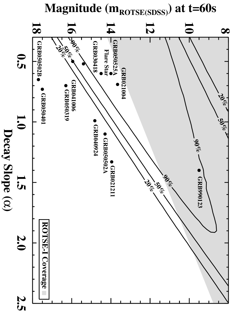
Figure 5.— Detection efficiency for fading transients, parameterized by their peak magnitude at $t=t_{0}+60$s, $m_{60}$, and their decay constant $\alpha$. The efficiencies calculated assume 30 minutes of effective coverage for each set for an integrated coverage of $1.74\,\mathrm{deg}^{2}\,\mathrm{yr}$. All sets with limiting magnitudes deeper than 17.5 were used for this plot. The contours describe our 20%, 50%, and 90% efficiency levels. The contours roll over at the bright end where many transients would be saturated and rejected. The gray area describes the coverage in the ROTSE-I transient search. Overplotted are approximate peak magnitudes and decay constants (averaged over the first hour) for six GRB afterglows with early detections. (Akerlof et al., 1999; Fox et al., 2003; Fox, 2004; Li et al., 2003; Rykoff et al., 2004b, 2005a, 2005b, 2005c; Yost et al., 2005; Falcone et al., 2005)

5. Discussion

To date, this is the deepest wide-field search for untriggered and orphan GRBs. With a total coverage of $1.74\,\mathrm{deg}^{2}\,\mathrm{yr}$, we have not found any candidate afterglows or other unknown transients. The primary reason we have been able to positively identify each of our transient candidates is the 5-color SDSS data of the fields in our search. Other transient searches such as the DLS that can image much deeper do not have this advantage.

We have also determined that the backgrounds for a search of this type are purely astrophysical. We have not had any difficulty from satellite glints or any mysterious terrestrial flashes. Our primary background consists of asteroids with small proper motion, but the MPChecker database combined with follow-up observations can eliminate these. Outside the solar system, but within the galaxy, we see a small but measurable rate of CVs and flare stars, as well as one extragalactic blazar. The flare star ROTSE3 J220806.9+023100.3 is the only object that we have found that had a light curve that mimicked our expected signature of an untriggered GRB afterglow.

We can place an upper limit on the rate of fading optical transients with quiescent counterparts dimmer than $\sim 20^{th}$ magnitude, as described by our 90% coverage region shown in Figure 5. To calculate an upper limit on the rate of transients in this region, we follow the method of Becker et al. (2004). The observed rate is

$$\eta=\frac{N}{{\langle}{\cal E}{\rangle}E}\,\mathrm{events}\,\mathrm{deg}^{-2}\,\mathrm{yr}^{-1},$$ (1)

where $N$ is the number of events, $E$ is the exposure, and ${\langle}{\cal E}{\rangle}$ is the efficiency. With the observed number of transients $N_{\mathrm{obs}}=0$, Poisson statistics place an upper limit of $N_{\mathrm{max}}<3.0$ with 95% confidence. Therefore, we can place a 95% confidence upper limit of $\eta_{\mathrm{max}}<1.9\,\mathrm{deg}^{-2}\,\mathrm{yr}^{-1}$ in our coverage region.

The launch of Swift will allow us to probe the early afterglow phase of GRBs far more systematically than has been achieved to date. We have learned some details from the variety of early afterglows detected so far. It is clear that very bright prompt flashes like that from GRB 990123 (Akerlof et al., 1999) are not the norm. It also appears that extrapolating late time afterglows to the early time generally over-predicts the brightness, as with GRB 030418 and GRB 030723. (Rykoff et al., 2004b) These data certainly make our search more difficult, as only $\sim 20\%$ of GRBs have afterglows that fall within our sensitivity region.

If we assume that the $\gamma$-ray emission of GRBs is confined within a double jet with a cone half-angle of $\theta_{\mathrm{max}}$, while the optical emission is isotropic, then a given GRB is visible in a small fraction of the sky approximated by $\theta^{2}/2$. Therefore, the true rate of GRB events within the observable universe must be $\sim 1500/\theta_{\mathrm{max}}^{2}\,\mathrm{events}\,\mathrm{yr}^{-1}$. The 95% confidence limit of $<78000\,\mathrm{events}\,\mathrm{yr}^{-1}$ is for a region that is sensitive to $\sim 20\%$ of GRBs, and therefore our assumption of isotropic optical emission is tenable as long as $\theta_{\mathrm{max}}>3.6^{\circ}$. As this is an approximate estimate of the GRB jet angle, the present limits cannot set stringent bounds on the properties of these objects. However, if programs such as ours continue to reduce the upper bounds for the orphan afterglow rate, the isotropic emission hypothesis will become incompatible with what we know about the structure of GRB jets. Although this is not an enormous surprise, it does represent a sanity check of the accepted model of GRBs by completely independent reasoning.

Our search has also detected several previously unknown high galactic latitude cataclysmic variables with dim quiescent counterparts. We have detected 3 new CVs with $\sim 52\,\mathrm{deg}^{2}\,\mathrm{yr}$ of coverage for slow decay transients that peak between $13^{th}$ and $16^{th}$ magnitude. This implies a rate of $0.06\,\mathrm{deg}^{-2}\,\mathrm{yr}^{-1}$. Assuming Poisson statistics, the 95% confidence upper limit on the rate is $0.17\,\mathrm{deg}^{-2}\,\mathrm{yr}^{-1}$. We have found 1 new CV with $\sim 25\,\mathrm{deg}^{2}\,\mathrm{yr}$ of coverage for CVs that peak between $16^{th}$ to $18^{th}$ magnitude. This implies a rate of $0.04\,\mathrm{deg}^{-2}\,\mathrm{yr}^{-1}$. Assuming Poisson statistics, the 95% confiedence upper limit on the rate is $0.21\,\mathrm{deg}^{-2}\,\mathrm{yr}^{-1}$. If we extrapolate the rate over the whole sky, this would produce $\sim 2000$ high galactic latitude CV outbursts every year. In the “Living Edition” catalog of CVs there are only $\sim 130$ CVs in our sensitivity range as of March 2005. (Downes et al., 2001) None of the CVs detected by ROTSE-III had been known previously. Our search results imply that many more CVs remain to be discovered.

The ROTSE-III transient search is an ongoing project. We expect to continue to patrol the sky over the lifetime of the Swift instrument (at least 2 years), as we wait for GRB triggers. We will thus gain another factor of 2-3 in coverage, and will achieve a modest improvement towards the goal of $\sim 110\,\mathrm{deg}^{2}\,\mathrm{yr}$, the threshold for having a high probability of finding an untriggered afterglow. In this paper, we have demonstrated that such a search is feasible, as the background rate of unknown transients is very low.

References

- Abazajian et al. (2005) Abazajian, K., et al. Mar. 2005, AJ, 129, 1755
- Akerlof et al. (1999) Akerlof, C., et al. 1999, Nature, 398, 400
- Akerlof et al. (2000) Akerlof, C., et al. Mar. 2000, ApJ, 532, L25
- Akerlof et al. (2003) Akerlof, C. W., et al. Jan. 2003, PASP, 115, 132
- Becker et al. (2004) Becker, A. C., et al. Aug. 2004, ApJ, 611, 418
- Bertin & Arnouts (1996) Bertin, E. & Arnouts, S. June 1996, A&AS, 117, 393
- Downes et al. (2001) Downes, R. A., Webbink, R. F., Shara, M. M., Ritter, H., Kolb, U., & Duerbeck, H. W. June 2001, PASP, 113, 764
- Falcone et al. (2005) Falcone, A., et al. 2005, GCN Circ. No. 3330
- Fenimore et al. (1993) Fenimore, E. E., et al. Nov. 1993, Nature, 366, 40
- Fox (2004) Fox, D. B. 2004, GCN Circ. No. 2741
- Fox et al. (2003) Fox, D. W., et al. Mar. 2003, Nature, 422, 284
- Frail et al. (2001) Frail, D. A., et al. Nov. 2001, ApJ, 562, L55
- Harrison et al. (1999) Harrison, F. A., et al. Oct. 1999, ApJ, 523, L121
- Kehoe et al. (2001) Kehoe, R., et al. 2001, ApJ, 554, L159
- Kehoe et al. (2002) Kehoe, R., et al. Oct. 2002, ApJ, 577, 845
- Lamb et al. (2004) Lamb, D. Q., et al. Apr, 2004, New Astronomy Review, 48, 423
- Lasker (1998) Lasker, B. M. May 1998, Bulletin of the American Astronomical Society, 30, 912
- Li et al. (2003) Li, W., Filippenko, A. V., Chornock, R., & Jha, S. Mar. 2003, ApJ, 586, L9
- Monet et al. (1998) Monet, D. B. A., et al. Oct. 1998, VizieR Online Data Catalog, 1252, 0
- Nakar & Piran (2003) Nakar, E. & Piran, T. Feb. 2003, New Astronomy, 8, 141
- Panaitescu & Kumar (2001) Panaitescu, A. & Kumar, P. Oct. 2001, ApJ, 560, L49
- Park et al. (1999) Park, H. S., et al. 1999, A&AS, 138, 577
- Rhoads (1997) Rhoads, J. E. 1997, ApJ, 487, L1
- Rykoff (2005) Rykoff, E. Jan. 2005, The Astronomer’s Telegram, 403, 1
- Rykoff & Quimby (2005) Rykoff, E. & Quimby, R. Feb. 2005, The Astronomer’s Telegram, 423, 1
- Rykoff et al. (2005a) Rykoff, E., Schaefer, B., & Quimby, R. 2005, GCN Circ. No. 3116
- Rykoff et al. (2004a) Rykoff, E. S., et al. Aug. 2004, Informational Bulletin on Variable Stars, 5559, 1
- Rykoff et al. (2004b) Rykoff, E. S., et al. Feb. 2004, ApJ, 601, 1013
- Rykoff et al. (2005b) Rykoff, E. S., Yost, S. A., & Smith, D. A. 2005, GCN Circ. No. 3165
- Rykoff et al. (2005c) Rykoff, E. S., Yost, S. A., & Swan, H. 2005, GCN Circ. No. 3465
- Stanek et al. (1999) Stanek, K. Z., Garnavich, P. M., Kaluzny, J., Pych, W., & Thompson, I. Sept. 1999, ApJ, 522, L39
- Vanden Berk et al. (2002) Vanden Berk, D. E., et al. Sept. 2002, ApJ, 576, 673
- Vestrand et al. (2004) Vestrand, W. T., et al. 2004, Astronomische Nachrichten, 325, 549
- Woudt et al. (2005) Woudt, P. A., Warner, B., & Rykoff, E. May 2005, IAU Circ., 8531, 3
- Yost et al. (2005) Yost, S. A., Swan, H., Schaefer, B. A., & Alatalo, K. 2005, GCN Circ. No. 3322