Pulse-phase spectroscopy of SMC X-1 with Chandra
and XMM-Newton: reprocessing by a precessing disk?

Abstract

We present pulse-phase X-ray spectroscopy of the high-mass X-ray pulsar SMC X-1 from five different epochs, using Chandra X-ray Observatory ACIS-S and XMM-Newton EPIC-pn data. The X-ray spectrum consistently shows two distinct components, a hard power law and a soft blackbody with $kT_{\rm BB}\sim 0.18$ keV. For all five epochs the hard component shows a simple double-peaked pulse shape, and also a variation in the power law slope, which becomes harder at maximum flux and softer at minimum flux. For the soft component, the pulse profile changes between epochs, in both shape and phase relative to the power law pulses. The soft component is likely produced by reprocessing of the hard X-ray pulsar beam by the inner accretion disk. We use a model of a twisted inner disk, illuminated by the rotating X-ray pulsar beam, to simulate pulsations in the soft component due to this reprocessing. We find that for some disk and beam geometries, precession of an illuminated accretion disk can roughly reproduce the observed long-term changes in the soft pulse profiles.

1. Introduction

The general picture of accretion onto X-ray pulsars, consisting of a flow in a disk to the magnetosphere and along the dipole field to the magnetic poles of the neutron star, has been known for decades (see Nagase, 1989, and references therein). However, despite extensive study, some important aspects of this process remain mysterious. In particular, the details of accretion near the magnetosphere, where the neutron star’s magnetic field begins to dominate the flow, is a complex and challenging problem (Elsner & Lamb, 1977; Ghosh et al., 1977; Ghosh & Lamb, 1978).

1.1. Superorbital variation in X-ray pulsars

One way to explore an accretion flow observationally is with systems where the shadow of the disk causes the X-ray source to vary with time. There are now $\sim$20 known accreting binary systems that exhibit superorbital periods, some of which are caused by shadowing of the source flux by an accretion disk (see Clarkson et al., 2003, and references therein). Of these systems, a small group of X-ray pulsars (SMC X-1, LMC X-4 and Hercules X-1) show luminous, pulsing X-ray emission which allows for study of the accretion flow in unusual detail. These systems each show a 30–60 d superorbital variation, attributed to a warped, precessing accretion disk (Tananbaum et al., 1972; Jones & Forman, 1976; Katz, 1973; Lang et al., 1981; Levine et al., 1996; Gruber & Rothschild, 1984; Wojdowski et al., 1998).

In the low-mass system Her X-1, the precessing disk has been studied extensively. Regular 35-day variations have been observed in the X-ray flux, pulse profiles, and spectrum, as well as optical and UV features (e.g., Vrtilek et al., 1994; Deeter et al., 1998, and references therein). In particular, occulation by the disk produces variations in the pulse profile shapes, which can be used to infer the overall warped disk geometry (Leahy, 2002; Scott et al., 2000).

SMC X-1 and LMC X-4 differ from Her X-1 in that they have high-mass (O and B star) companions, hence we expect the accretion mechanism to be somewhat different due to the presence of powerful stellar winds. However, the high X-ray luminosities of SMC X-1 and LMC X-4 ($>10^{38}$ ergs s^-1) require Roche lobe overflow in addition to accretion from the wind, and there is evidence for persistent, warped accretion disks.

For example, in LMC X-4, precession of the disk is believed to cause changes in the X-ray power-law slope and flourescent iron line flux as a function of superorbital phase (Naik & Paul, 2003, 2002), as well as variations in the ultraviolet spectra (Preciado et al., 2002). For SMC X-1, observations of X-ray spectra (Wojdowski et al., 1998) and photoionized lines in the UV and X-ray (Vrtilek et al., 2001, 2005) give evidence for shadowing of the central neutron star by the precessing disk. From the observed line features, Vrtilek et al. (2005) conclude that the occulation of the source is caused by the inner regions of the disk, near the magnetospheric radius $\sim$$10^{8}$ cm.

1.2. Disk reprocessing and the soft X-ray emission

In Her X-1, reprocessing of the hard X-rays from the neutron star by the inner accretion disk produces a soft ($<1$ keV) X-ray component that pulses out of phase with the hard ($>2$ keV) pulses (e.g. Endo et al., 2000; Ramsay et al., 2002). Thus the X-ray beam from the neutron star acts as a “flashlight” that illuminates the inner disk (Fig. 1).

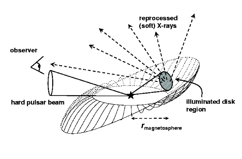
Figure 1.— Schematic of disk reprocessing in X-ray pulsars. The hard (power law spectrum) X-ray beam sweeps around and illuminates the accretion disk, which re-radiates a soft X-ray (blackbody) component. The observer sees pulses from both the power law and blackbody components, but these differ in pulse shape and phase.

Many luminous X-ray pulsars, including LMC X-4 and SMC X-1, have similar soft spectral components that are likely also caused by disk reprocessing (Hickox et al., 2004). We expect the flux of such a soft component to pulsate as the pulsar beam sweeps around and illuminates the disk. The soft pulses will have the same period as those from the hard X-ray beam, but will have a different shape and relative phase. Moreover, precession of the accretion disk will change the observer’s view of the inner region, and so the shape and phase of the reprocessed component should vary with superorbital period. Hints of such an effect have been seen in Her X-1: Zane et al. (2004) showed using XMM data that the phase offset between the soft (0.3–0.7 keV) and hard (3–10 keV) pulse profiles vary with time, and appears to be correlated with precession of the disk. A soft component that pulsates separately from the hard component has also been seen in LMC X-4 (Naik & Paul, 2004b) and SMC X-1 (Paul et al., 2002; Naik & Paul, 2004a).

1.3. SMC X-1

SMC X-1 was first identified as a point source in Uhuru observations by Leong et al. (1971). Eclipses were discovered by Schreier et al. (1972) and X-ray pulsations by Lucke et al. (1976). The optical counterpart is Sk 160, a B0 I supergiant (Webster et al., 1972; Liller, 1973). The orbit is close to circular, with orbital period $\sim$3.9 days and pulse period 0.7 s. The source has a high X-ray luminosity, $L_{\rm X}\sim 3\times 10^{38}$ ergs s^-1, in the bright state.

In SMC X-1 the period of the superorbital cycle oscillates from 40 to 60 days (Wojdowski et al., 1998), a variation that may itself be periodic on the order of years (Clarkson et al., 2003). The high-state, out-of-eclipse X-ray spectrum is usually fitted as a cutoff power law with $\Gamma\sim 0.9$, an iron line at $\sim$6.4 keV, and a soft component modeled as a broken power law, thermal bremsstrahlung, or a blackbody with $kT_{\rm BB}\sim 0.16$ keV. Paul et al. (2002) fit four different models to the soft component and found that all gave satisfactory fits. They found that the soft component flux pulses roughly sinusoidally, out of phase with the sharper-peaked pulses from the power law. Neilsen et al. (2004) created hard and soft pulse profiles for ROSAT, Chandra, and XMM data of SMC X-1, and found that for different epochs the the soft pulse shapes vary while the hard pulses remain similar.

In this paper we seek to explore the variation in these spectral components further, by performing pulse-phase spectroscopy for SMC X-1 at several epochs. We have also constructed a model to simulate hard and soft pulse profiles that would be produced by an X-ray pulsar beam illuminating a warped, precessing accretion disk, and compare the results with observations.

2. Observations and data reduction

Figure 2.— RXTE ASM lightcurve for SMC X-1 with arrows designating several observations. Quick-look results as provided by the RXTE/ASM team.

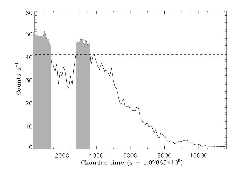
Figure 3.— XMM EPIC-pn light curve (0.15–12 keV) for observation X101, showing entrance to eclipse. Times with flux $>41$ cts s^-1 (shaded) were included in the spectral analysis.

We have used three Chandra and two XMM observations of SMC X-1, taken in the high state of the superorbital cycle. Details of the observations are given in Table 1. Pulse profile analysis for these data are presented in Neilsen et al. (2004), and we will use their abbreviations to denote the observations (C102, X101, etc.). Fig. 2 shows the observations on the long-term light curve of SMC X-1 from the All Sky Monitor (ASM) on RXTE. From this we estimate the superorbital phases given in Table 1, taking $\phi_{\rm SO}=0$ at the start of the superorbital high state. These estimates have uncertainty of $\pm$ a few days or $\phi_{\rm SO}\sim 0.05$, because the superorbital intensity variation in SMC X-1 is quasi-periodic in nature and hence does not have a well-defined ephemeris.

Table 1Chandra and XMM observations of SMC X-1

Observation ID	Mission	Start Time	Total	$\phi_{\rm orb}$	$\phi_{\rm SO}$	Fluxes ($10^{-10}$ ergs cm-2 s-1)
(Reference)		(JD-2400000)	Exp. (ks)			Power law	Blackbody	Total
400102 (C102)	Chandra	51832.17	06.2	0.19	0.16	9.3	0.9	10.2
400103 (C103)	Chandra	51833.34	06.1	0.49	0.16	9.1	1.6	10.7
400104 (C104)	Chandra	51834.31	06.5	0.74	0.16	9.2	1.4	10.6
0011450101 (X101)	XMM	52060.59	27.9	0.89	0.37	6.5	0.4	6.9
0011450201 (X201)	XMM	52229.65	01.6	0.34	0.42	10.1	1.3	11.4

The Chandra observations were each $\sim$6 ks in duration, and they were taken with the ACIS-S3 chip in Continuous Clocking (CC) mode, in which charge is continually read out down the chip. This allows for 3.5 ms time resolution, but one dimension of spatial information is lost so that the X-ray image is simply a straight line. There are no other bright sources within the ACIS field of view near SMC X-1, so we can determine source and background regions from the 1-D image and extract events normally. For each observation the source region was a rectangle of size $0\farcs 49\times 1\farcs 97$ centered on the source. Background events came from two rectangles $0\farcs 49\times 9\farcs 84$ on either side of the source.

For the XMM observations we have used data from the EPIC-pn CCD camera, which has the highest time resolution of the EPIC cameras. X201 had a clean exposure of $\sim$27 ks in duration, and was taken in Small Window mode, which has 6 ms time resolution. For this observation we have extracted source events from a circle of radius $51\farcs 2$. X101 was taken in Full Window mode, which has 73.5 ms time resolution. While the total exposure for X101 was 40 ks, the bulk of this observation was during full eclipse, with only the first few ks showing substantial flux. Neilsen et al. (2004) analyzed the first 4.9 ks of data, which consisted of the entire entrance into eclipse. However, they found that a partial covering absorption model was needed to explain the X-ray spectrum, perhaps due to occultation by the outer layers of the star. To avoid this complication, we restricted the present analysis to the 1.6 ks of data for which the 0.15-12 keV count rate was $>41$ counts s^-1 (see Fig. 3). The background surface brightness for the XMM data was $<0.1$% of the source brightness, so we did not perform background subtraction.

3. Data Analysis

3.1. Dealing with event pileup

In high count-rate data such as these, the X-rays measured by CCD detectors are affected by pileup, caused when two or more photons are coincident on one event-detection cell during one time-resolution element, or frame time (Davis, 2001). In this case the detector cannot distinguish the multiple events and instead detects a single event with a pulse height roughly equal to the sum of the pulse heights from the individual photons. Pileup has several effects on the detected X-ray events, most importantly that the overall detected count rate is lowered, and the spectrum is shifted from lower to higher energies, due to the absence of real lower energy events and the addition of “fake” higher-energy events.

There is also an effect on the “grade” of the detected events. The grade of an X-ray event is a number that refers to how the charge cloud from a photon hitting a CCD pixel is spread across neighboring pixels. Real X-ray events have characteristic grades that can be used to distinguish them from unwanted events such as particle background interactions. However, when two or more photons are piled up, they often result in grades that do not match those of individual photons, and so are thrown away by this filtering, thus decreasing the count rate. Taking into account this “grade migration” is an important part of modeling pileup. For a discussion of these effects in detail, see Davis (2001).

In this study we deal with pileup in three different ways: short frame times, excluding events from the center of the PSF (for XMM), and pileup modeling (for Chandra). All five observations have short frame times $<$75 ms, which mitigate pileup by reducing the likelihood that multiple photons will be coincident in one time resolution element.

For the XMM data, we tested for pileup using the SAS tool epatplot, which compares the distribution of events of different grades with that expected for no pileup. When events from the full PSF were included, these distributions differed significantly, indicating pileup. However, because count rates (and thus pileup effects) are greatest at the center of the PSF, we found that by excluding events from the central 1/3 radius of the source region, we could eliminate any significant pileup effects.

For the Chandra data we could not simply exclude the inner extraction region. Because the PSF is smaller than for the XMM  and because the use of CC mode concentrates all the events along one dimension, most source events are concentrated in a few pixels. Therefore, we fit the data in the ISIS package using the pileup kernel, which models and corrects for pileup effects in spectral fitting (Davis, 2001). This kernel includes a grade migration parameter $\alpha$ which can be allowed to float to best characterize the effect that pileup has on the grade selection of the observation. On average 17% of the photons in the ACIS spectra are piled up. This level of pileup can be corrected using the ISIS kernel while measuring the spectral parameters.

3.2. Pulse-phase spectroscopy

Pulse phase-resolved spectra were extracted in the range 0.6–10 keV. For the Chandra data we excluded the energy range 1.7–2.8 keV in our spectral fits (as in Neilsen et al., 2004), to avoid instrumental effects near the Au and Si edges. For both XMM and Chandra, we cleaned the data for flaring episodes before spectral extraction.

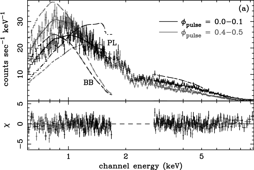
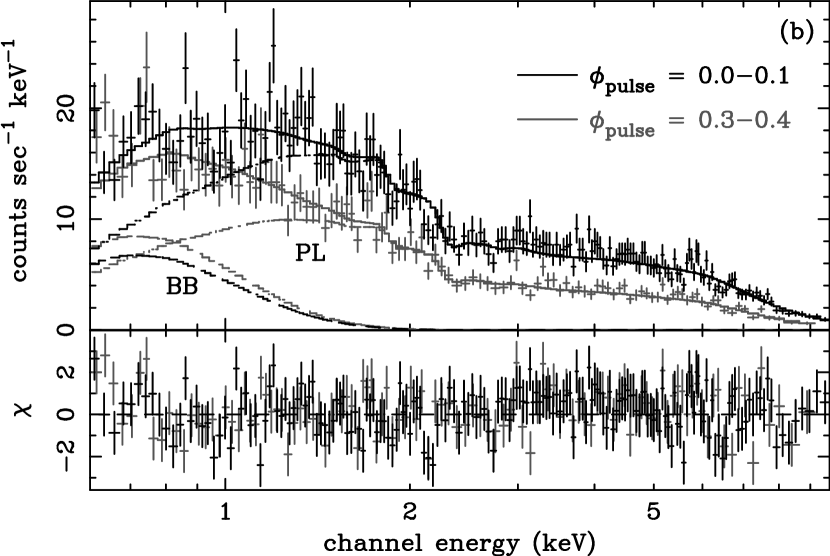
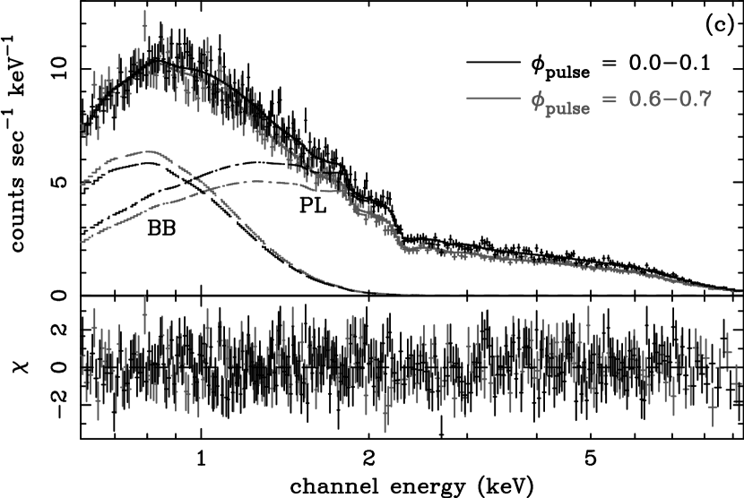
Figure 4.— Pulse phase-resolved spectra for SMC X-1, for (a) C103 (b) X101, (c) X201. For each observation two spectra are shown, from pulse phases that show substantial differences in the spectral parameters. The individual blackbody (BB) and power law (PL) components are also shown. In the Chandra data, these individual components do not add to the total, because of the effect of the pileup model. Also note that the energy range 1.7–2.8 keV was excluded from the Chandra fits.

The best fit spectral models for the Chandra and XMM observations consisted of a power law ($\Gamma\sim 0.9$) plus blackbody $kT_{\rm BB}\sim 0.18$, both modified by neutral absorption. We also included a high-energy exponential cutoff on the power law, as has been seen in Ginga and ASCA observations (Woo et al., 1995; Paul et al., 2002). X201 was the only observation with sufficient high-energy counts to constrain this cutoff, so for the other observations we fixed the parameters to the phase-averaged value for X201 ($E_{\rm cut}=6.1$ keV and $E_{\rm fold}=6.8$ keV). The models can be written as:

Chandra:

$f(E)=K_{\rm pile}\otimes{e^{-\sigma(E)N_{\rm H}}[f_{\rm BB}(E)+f_{PL}(E)f_{\rm cut}(E)]}$

XMM:

$f(E)=e^{-\sigma(E)N_{\rm H}}[f_{\rm BB}(E)+f_{PL}(E)f_{\rm cut}(E)]$

where $f_{\rm BB}$, $f_{PL}$, $f_{\rm cut}$, are the standard XSPEC blackbody, power law, and high-$E$ cutoff models. $K_{\rm pile}$ is the ISIS pileup kernel.

In general, for phase-averaged spectral parameters we use the results of fits by Neilsen et al. (2004). However for X101 we performed a new phase-averaged fit, because we have revised the time interval over which the spectrum was extracted (see § 2). We fixed the high-energy cutoff as above, giving $N_{\rm H}=1.3\times 10^{21}$ cm^-2, $kT_{\rm BB}=0.17$ keV, and $\Gamma=0.79$, with XSPEC normalizations $K_{\rm BB}=8.8\times 10^{-4}$ (in units of $8.3\times 10^{-8}$ ergs cm^-2 s^-1) and $K_{\rm PL}=3.5\times 10^{-2}$ (photons keV^-1 cm^-2 s${-1}$ at 1 keV).

To extract phase-resolved spectra, we first corrected the photon arrival times for the motion of the Earth and the observatory, as well as the orbital motion of SMC X-1 using the ephemeris found by Wojdowski et al. (1998). Using the pulse periods found by Neilsen et al. (2004), we extracted spectra in 10 bins of $\phi_{\rm pulse}$ for each of the observations. We fit the spectra in ISIS for Chandra and XSPEC for XMM, using the models given above. For the Chandra fits, we fixed the grade migration parameter $\alpha$ at its phase-averaged value.

Figure 5.— Pulse phase variation of spectral parameters for SMC X-1, for (a) Chandra: solid: C102, dashed: C103, dot-dashed: C104 (b) X101, (c) X201. Shown are the relative fluxes from the power law and blackbody components, the power law index $\Gamma$, and the blackbody temperature $kT_{\rm BB}$ in keV (note that the temperature was fixed in the X101 fits). Two pulses are shown for clarity. Errors are 1$\sigma$, and typical error bars for Chandra are given to the left of the plots. The average fluxes in the power law and blackbody components are given in Table 1.

For each fit we set the initial parameters to the phase-averaged values, and fixed the $N_{\rm H}$ and high energy cutoff while allowing the other parameters to vary. For X101, the limited statistics required that we also fix the blackbody temperature, $kT_{\rm BB}$, in order to measure the variation in the soft component. Sample phase-resolved spectra for C103, X101, and X201 are shown in Fig. 4, for which changes in shape between spectra at different $\phi_{\rm pulse}$ are clearly visible. The phase-resolved fits have $\chi^{2}_{\nu}$ values of 0.8–1.0 for Chandra, 1.0–1.3 for X101, and 0.9–1.2 for X201.

We found that the best-fit spectral parameters vary significantly with $\phi_{\rm pulse}$. For each phase we calculated the 0.5–10 keV unabsorbed flux in both the blackbody and (cutoff) power law components. The $\phi_{\rm pulse}$ variation of the fluxes, along with $\Gamma$ and $kT_{\rm BB}$, are shown in Fig. 5. We find that:

1. At every epoch, the power law flux shows the familiar double peaked profile, similar to the hard pulse profile observed many times previously. The phase offset and relative intensities of the two peaks vary slightly between epochs.

   

   Figure 6.— Pulse-phase variation in spectral parameters for C103, using a blackbody (histogram) and a thermal bremsstrahlung (dashed line) soft component model. Note that the hard and soft flux profiles do not differ significantly for the two models.

2. The power law photon index varies significantly, inversely with the power law flux. The spectrum gets harder as the power law flux increases, and softer as the flux decreases.

3. For all observations, the blackbody flux shows a single main peak, and in the Chandra observations there is a shoulder after the main peak.

4. The shapes and relative phases of the blackbody pulses change with time. However the three Chandra observations (at $\phi_{\rm orb}=0.19$, 0.49, and 0.74) have very similar soft pulses. This implies that the changes in the soft profiles are not correlated with orbital motion of the source, and occur on timescales longer than a few days.

To test whether the observed variation is dependent on the particular choice of soft component model, we repeated the pulse-phase spectroscopy using a thermal bremsstrahlung (TB) model in place of the blackbody. This fits are acceptable for $kT_{TB}\sim 0.3$ keV, with very similar $\chi^{2}$ to the blackbody fits. This is not a physical model, because a large, diffuse thermal gas cloud could not produce the luminous, pulsing soft emission observed (Hickox et al., 2004), but it allows us to check that the measurement of variation in the soft component is robust. The soft and hard component flux profiles for this model for one observation (C103) are given in Fig. 6, and are compared to those for the blackbody model. The shapes of the profiles differ by $\lesssim 0.5\sigma$, for the two models, except for the soft profile in C102, for which they differ by $\simeq 1.2\sigma$. Since these differences are not highly significant, we conclude that the hard and soft flux profiles are essentially independent of the model chosen for the soft component.

4. Photon index variation

The observed changes in the power law index with pulse phase have not been previously reported for SMC X-1; the ASCA study of Paul et al. (2002) found that $\Gamma\simeq 1.0$ for four different pulse phases. We have investigated the possibility that this variation may not be real, but an instrumental effect due to pileup. This is possible in principle because pileup increases with flux and serves to lower soft count rates and increase hard count rates, any residual pileup for which we have not accounted could cause a “hardening” of the spectrum as flux increases. However after detailed testing we conclude that the variation is not due to pileup effects, because:

1. Modeling of pileup in the Chandra data using the ISIS pileup kernel (Davis, 2001) shows that the $\sim$50% changes in the flux that we observe can only change the power law slope by 0.01, which is much smaller than the observed variation in the Chandra spectrum.

2. Variation in $\Gamma$ is also observed in the XMM observations, for which piled-up events have been removed. If we use all the events (including piled-up ones) in the X201 analysis, we find that the average value of $\Gamma$ is flatter by $\sim$0.1 due to pileup effects, but the variation in $\Gamma$ of $\pm$0.5 remains the same.

Therefore the pulse variation in the power law index appears to be independent of any pileup. We treat this effect as real and consider physical interpretations.

Power-law index variation with pulse phase has been observed in a number of X-ray pulsars. We searched the sample of bright pulsars in Table 2 of Hickox et al. (2004) for those with existing pulse-phase spectroscopy. We find that many sources show variations in $\Gamma$, and these tend to be correlated with the pulse intensity. Some sources, such as LMC X-4 (Woo et al., 1996), Cen X-3 (Burderi et al., 2000), Vela X-1 (Kretschmar et al., 1997), and 4U 1626–67 (Pravdo et al., 1979), become harder with increasing intensity, as we have observed for SMC X-1. However, Her X-1 (Ramsay et al., 2002), V0332+53 (Unger et al., 1992), and 4U 1538–52 (Clark et al., 1994) become softer with increasing flux. XTE J0111.2–7317 (Yokogawa et al., 2000), RX J0059.2–7138 (Kohno et al., 2000) , and GX 301–2 (Endo et al., 2000) show no variation in $\Gamma$.

Because of this variety of behaviors, it is difficult to present a universal physical picture for the pulse-phase changes in the power law spectra of X-ray pulsars. In the standard picture of spectral formation in luminous pulsar beams, the accretion column is stopped by a radiatively driven shock. If photons in the brightest part of the beam are generated in strongest shock, they will have been scattered with larger Compton $y$ parameter and so preferentially emerge at higher energies. This would make the center of the pulse harder and the outside softer, as observed for SMC X-1. A mechanism for a softening with pulse flux is not immediately clear. We would like to stress, however, that variation in $\Gamma$ with pulse phase is very common, and so must be addressed by successful models of X-ray pulsar spectral formation.

5. Reprocessing by a warped disk

The soft component pulses observed are roughly consistent with the picture argued by Hickox et al. (2004) and Neilsen et al. (2004) that double-peaked power law pulses come from near the neutron star’s accreting polar caps, while the soft pulses come from a much larger radius, at the irradiated inner region of the accretion disk.

We seek to test this possibility by comparing the observed hard and soft pulse profiles to a relatively simple model, in which a warped, twisted inner accretion disk is illuminated by a rotating X-ray pulsar beam.

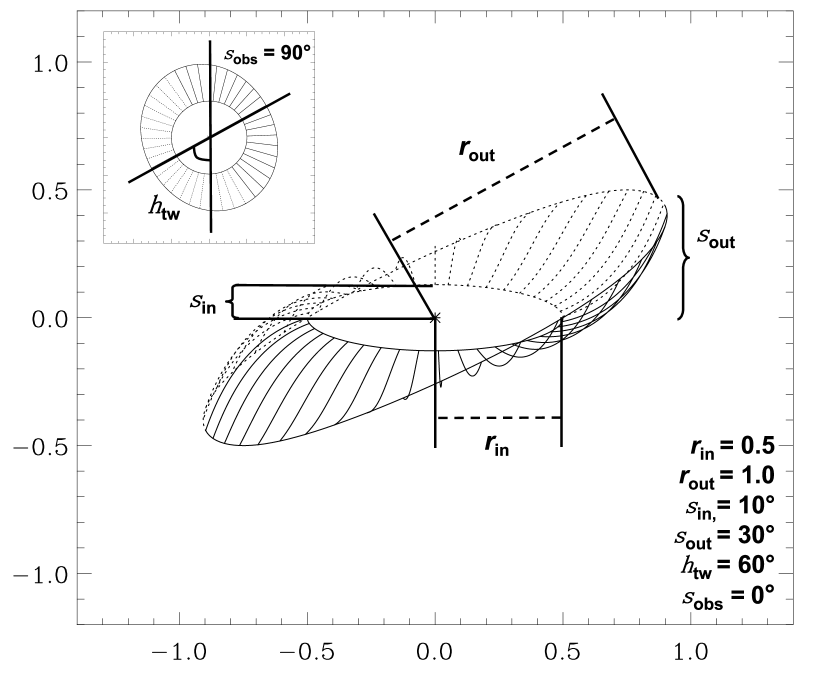
Figure 7.— Diagram of the twisted disk model, showing the relevant parameters. The disk is viewed at elevation $\theta_{\rm obs}=0^{\circ}$. Inset: the same disk viewed at $\theta_{\rm obs}=90^{\circ}$, showing the disk twist angle $\phi_{\rm tw}$.

5.1. Illuminated disk model

Our model does not describe the entire disk, but only the region close to the magnetosphere where the bright reprocessed component must be emitted. The disk model consists of a series of concentric circles with varying tilt and twist relative to each other with distance from the center (see Fig. 7. A similar shape has been inferred for the large-scale structure of the disk in Her X-1, from changes in the pulse profiles with superorbital phase (Scott et al., 2000; Leahy, 2002). Warped and twisted structures have also resulted from numerical simulations of warped disks (Wijers & Pringle, 1999) and of gas-magnetosphere interaction (Romanova et al., 2003).

Table 2Parameters for disk models

	Model ranges		Best fit
Parameter	Pencil beam	Fan beam	Pencil beam	Fan beam
$L_{X}$ (ergs s-1)	$3\times 10^{38}$	$3\times 10^{38}$	$3\times 10^{38}$	$3\times 10^{38}$
$R_{\rm in}$ ($10^{8}$ m)	0.8	0.8	0.8	0.8
$R_{\rm out}$ ($10^{8}$ m)	1	1	1	1
Outer angle $\theta_{\rm out}$ (deg)	30	30	30	30
Inner angle $\theta_{\rm in}$ (deg)	10	10	10	10
Twist angle $\phi_{\rm tw}$ (deg)	-90, 90, 135	90	90	90
$\theta_{\rm b1}$ (deg)	35, 45	0, 45	35	45
$\theta_{\rm b2}$ (deg)	-10, 0, 10, 20	0, 45	-10, 10	0
$\phi_{\rm b1}$ (deg)	0	0	0,	0
$\phi_{\rm b2}$ (deg)	210, 225, 240	180, 210, 225	225, 210	180, 210
Beam half-width $\sigma_{\rm b}$ (deg)	30	15	30	15
Fan opening angle $\theta_{\rm fan}$ (deg)	0	45, 60, 90	0	60
Observer elevation $\theta_{\rm obs}$ (deg)	20	20	20	20

In our calculations we place this surface (we will refer to it simply as the “disk”) at roughly the location of the magnetosphere ($\sim$$10^{8}$ cm), and test if precession of such a surface around the disk axis can create changing soft-component profiles similar to those observed. The shape of the surface is determined by the radii and tilt angles of the inner and outer circle ($r_{\rm in}$, $r_{\rm out}$, $\theta_{\rm in}$ and $\theta_{\rm out}$), and the offset angle or “twist” between them ($\phi_{\rm tw}$). Letting $\theta_{\rm d}$ be the angle of the disk above the rotation plane at any point ($r,\phi$), we use the simple approximation:

$$\theta_{\rm d}(r,\phi)=-(\theta_{\rm in}+(\theta_{\rm out}-\theta_{\rm in})\frac{r-r_{\rm in}}{r_{\rm out}-r_{\rm in}})\sin{(\phi-\phi_{\rm tw})},$$

which is valid for $\theta\lesssim 30^{\circ}$.

It is also necessary to define a beam pattern from the neutron star. Complex beam shapes have been proposed for some X-ray pulsars; for example Her X-1’s emission has been modeled as a central pencil beam surrounded by a fan beam (Blum & Kraus, 2000), or even a reverse-pointing fan beam, emitted from above the neutron star’s surface (Scott et al., 2000). However, since we are modeling coarse pulse profiles with only 10 bins of pulse phase, it is impossible to constrain such complex models, so we use a simple beam shape.

The beam is described by two two-dimensional gaussians, superposed on an isotropic component which is required since the hard pulse fraction for SMC X-1 is only $\sim$50%. We define the beam pattern in spherical coordinates, with the poles aligned with the rotational axis and $\theta=0$ at the equator. We set the neutron star’s rotation to be parallel to the disk axis. Each gaussian is specified by its width ($\sigma_{\rm b}$), its angle from the rotational plane ($\theta_{\rm b}$), and its azimuthal angle ($\phi_{\rm b}$). We also define a fan opening angle ($\theta_{\rm fan}$), which we set to zero to model “pencil” beams, and to $\geq 45$^∘ to model “fan” beams.

We set the peak intensity of each gaussian equal to 3 times the intensity of the isotropic component. Note that this normalization is somewhat arbitrary; when we fit the output model profiles to the data we allow the intensity of the pulses to vary. The beam pattern is given by:

$$F_{\rm b}(\theta,\phi)=1+3e^{-(\alpha_{1}-\theta_{\rm fan1})^{2}/2\sigma_{1}^{2}}+3e^{-(\alpha_{2}-\theta_{\rm fan2})^{2}/2\sigma_{2}^{2}}$$

where $\alpha_{1,2}$ is the angular distance between ($\theta,\phi$), and ($\theta_{\rm b1,2},\phi_{\rm b1,2}$). This beam pattern is normalized to a total hard emission luminosity of $L_{\rm X}=3\times 10^{38}$ ergs s^-1.

This beam pattern is then swept around the disk. We take the disk to be opaque and calculate the luminosity absorbed by each patch of the disk surface. We assume that all this energy is re-radiated as a blackbody spectrum, with temperature

$$T=(\textrm{d}L/(4\pi\sigma\textrm{d}A))^{1/4}.$$

Only those regions of the disk that are directly visible from the neutron star are illuminated. Finally, we calculate which of the illuminated regions are visible to the observer, and are not blocked by parts of the disk in front.

We assume that the heated disk immediately re-radiates its thermal energy, so that there is no time lag between illumination by the X-ray beam and emission from the disk. This assumption requires that both the light-crossing time for the system and the cooling time for the heated disk are much shorter than the pulse period. In our model the illuminated region is at $R\sim 10^{8}$ cm, so the light crossing time is $\sim$10 ms.

A rough estimate for the cooling timescale is given by Endo et al. (2000), and is simply the total thermal energy of the heated disk divided by its luminosity. The disk’s thermal energy is the volume of the heated region times its thermal energy density. If we treat the disk as a partial spherical shell presenting solid angle $\Omega$ to the neutron star, we have

$$E_{\rm BB}=\Omega 4\pi R_{\rm BB}^{2}d\left(\frac{3}{2}nkT_{\rm BB}\right),$$

where $d$ is the penetration depth of hard X-rays into the heated region. We assume that most X-rays penetrate no more than a few Compton depths, so that $nd\sim 3/\sigma_{\rm T}\sim 10^{25}$ cm^-2. For $R_{\rm BB}=10^{8}$ cm, $\Omega/4\pi\sim 0.1$, and $kT_{\rm BB}=0.18$ keV, we have $E_{\rm BB}\sim 10^{32}$ erg. The cooling timescale is simply $t_{\rm cool}=E_{\rm BB}/L_{\rm soft}$, which for $L_{\rm soft}\sim 10^{37}$ ergs s^-1 gives $t_{\rm cool}\sim 10^{-5}$ s.

Since both these timescales are much shorter than the pulse period, we can treat the reprocessing as instantaneous. For each neutron star rotation phase, we calculate the total luminosity visible to the observer for the hard emission from the neutron star, appropriate to the observer’s view of the given beam pattern. We also sum the observable reprocessed emission from the disk. We thus obtain “hard” and “soft” model pulse profiles that we can compare to observations.

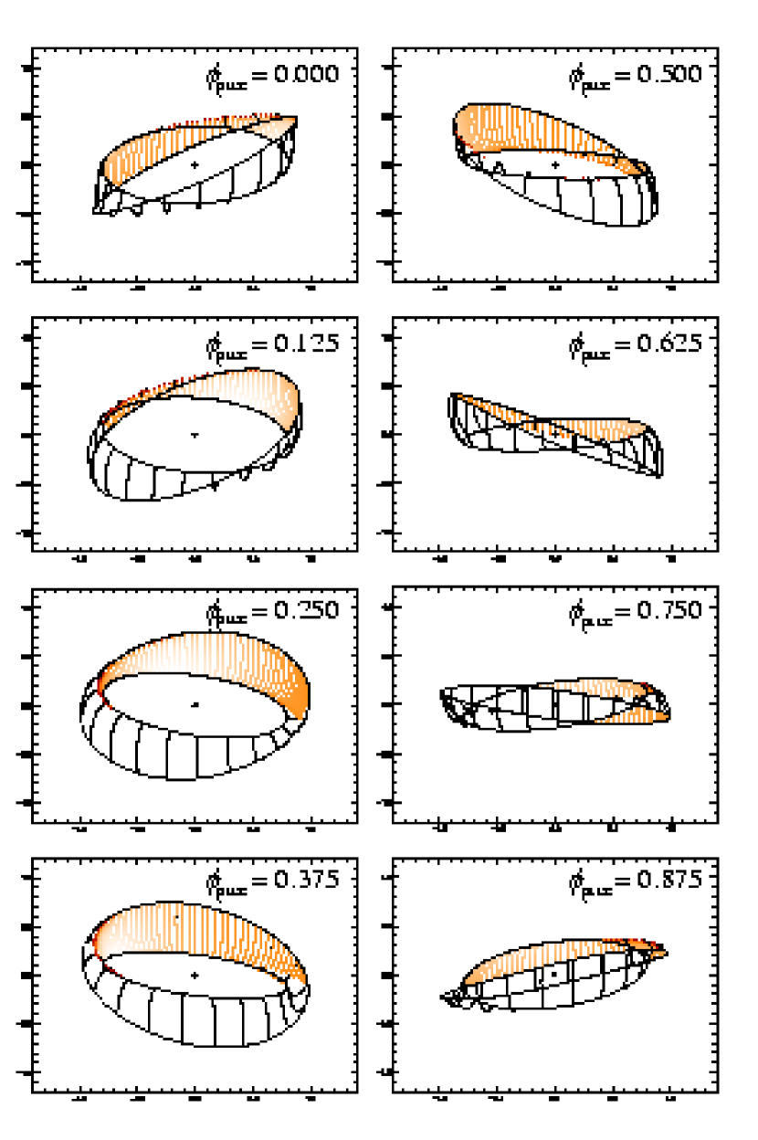
Figure 8.— Model twisted, tilted accretion disk as used in our reprocessing calculations. Shown is the model which allows the best fit to the observed (see Table 2). The shaded regions show areas on the disk which are illuminated by the central source and are visible to the observer. Lengths are in $10^{8}$ cm.

5.2. Model output

We have created a number of illuminated disk models, varying the disk shape ($\theta_{\rm in},\theta_{\rm out},\phi_{\rm tw}$), the beam pattern ($\theta_{\rm b1},\theta_{\rm b2},\phi_{\rm b2},\theta_{\rm fan}$), and the observer’s elevation angle $\theta_{\rm obs}$. Because the model is computationally intensive, we did not perform a systematic study of the whole range of possible configurations. We initially ran the model for a broad variety of disk shapes and beam patterns, then limited our systematic study to those parameters that could roughly reproduce the observed properties of SMC X-1. These parameter ranges are given in Table 2. We set the outer disk to be inclined at 30^∘, which is consistent with disk inclination estimates of 25^∘–58^∘(Lutovinov et al., 2004), and set the inner disk at a somewhat smaller inclination of 10^∘. This disk shape results in 20–30% of the neutron star luminosity being reprocessed. We set the elevation angle of the observer, with respect to the neutron star’s rotation plane, to be $\theta_{\rm obs}=20$^∘. If the neutron star spins in the plane of its orbit, this corresponds to an orbital inclination $i=70$^∘. This is consistent with the estimated range of $i\simeq 65$–70^∘ from optical studies, assuming approximately Roche geometry for the companion star (Reynolds et al., 1993; Hutchings et al., 1977). To obtain the observed blackbody temperature of $\sim$0.18 keV, we placed the reprocessing region between $r_{\rm in}=0.8\times 10^{8}$ cm and $r_{\rm out}=1\times 10^{8}$ cm.

The model disks consisted of a grid on $(r,\phi)$ of 100 elements in each dimension. For each disk shape we calculated the emission at 30 separate pulse phases and 8 disk precession phases. The observer’s views of the disk at several precession phases are shown in Fig. 8. In the upper left panel of Fig. 8, the neutron star has just emerged from behind the precessing disk, which corresponds to the start of the high superorbital intensity state for which $\phi_{\rm SO}=0$. Therefore we set $\phi_{\rm prec}=0$ for this model disk orientation and define the other precession phases accordingly. For each model beam and $\phi_{\rm prec}$, we calculated the observed pulse profiles for the direct emission from the neutron star (the hard profile) and the reprocessed emission from the disk surface (the soft profile).

5.3. Pencil beam models

We begin by examining pencil beam shapes, for which $\theta_{\rm fan}=0$. To reproduce the hard pulse profiles observed, we found that the two beams could not be anitipodal, that is $\theta_{\rm b1}\neq\theta_{\rm b2}$ and $\phi_{\rm b2}\neq 180$^∘(with $\phi_{\rm b1}=0$^∘). The observed hard pulse peaks are not exactly 180^∘ out of phase, so we varied $\phi_{\rm b2}$ between 210^∘ and 240^∘. To produce the relative heights of the two hard pulses, we set $\theta_{\rm b1}$ to 35^∘ or 45^∘ and varied $\theta_{\rm b2}$ between -10^∘ and 20^∘.

While these represent only a small subset of the possible disk/beam configurations, they allow us to test whether, in principle, reprocessing by a precessing disk can reproduce the observed pulse profiles. The model results for pencil beams show that:

1. Most disk configurations display some kind of variation in the shape and phase of the pulses in the soft, reprocessed component.

2. The relative shapes of the hard and soft pulses vary most strongly with the shape of the illuminating beams, and less strongly with the detailed shape of the disk.

For our array of models, we performed $\chi^{2}$ fits of the model pulses to the observed power law and blackbody flux profiles (shown in Fig. 5) for each observation. We allowed the normalization of the calculated pulses to vary, in order to account for any differences in pulse fraction between the observed pulses and our model.

For each model we first fit the hard profiles to the observed power-law profiles, allowing the scale and the phase offset of the model profiles to vary. This achieved a reasonable fit ($\chi^{2}_{\nu}\lesssim 2$) for many pencil-beam models. We next attempted to fit the blackbody pulses by varying only the amplitude of the model profiles; the phase was fixed to that from the hard profile fit. For most model parameters, the shape and phase offset of the model soft pulses do not match those in the data, and no good fit is achieved.

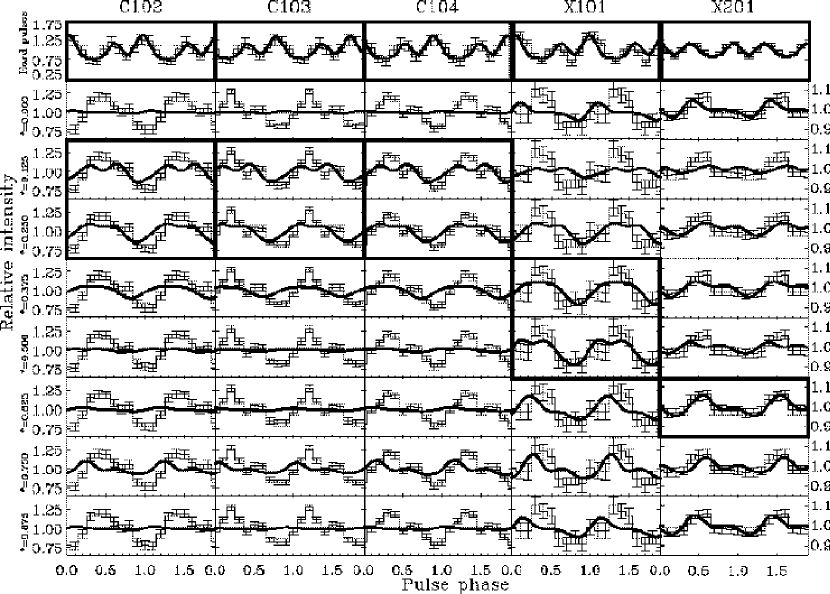
Figure 9.— Hard and soft pulse profiles output by the disk reprocessing model, fitted to the observed profiles for the five observations. The disk and beam parameters are given in Table 2. Each column shows observed spectral component pulses (as in Fig. 5) from one of the five observations. The top row shows the power law profiles fitted by the pulses from the neutron star, and the lower rows show blackbody profiles fitted by the model reprocessed pulses. Reprocessing for 8 disk precession phases $\phi_{\rm prec}$ are shown. Note that the observed soft pulses vary in phase and shape with $\phi_{\rm prec}$. Highlighted in bold are the profiles that best fit for the observed power-law pulses (top) and reprocessed pulses (below). This disk and beam configuration fits the Chandra data best at $\phi_{\rm prec}=0.125$–0.25 and X101 best at $\phi_{\rm prec}=0.375$–0.5. The X201 pulses require a slightly different beam pattern (see Table 2) and fit the data well for $\phi_{\rm prec}=0.625$. Note that the X201 soft pulses are weaker than the other four, and are shown using a different scale.

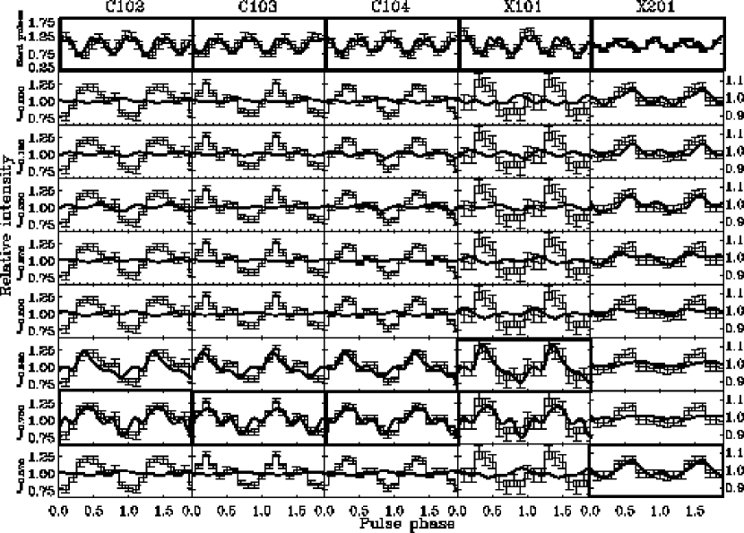
Figure 10.— Same as Fig. 8, for a fan rather than a pencil beam shape. The profiles correspond to the fan beam configuration that best fit the observations, with parameters given in Table 2.

However, for one particular disk shape (Fig. 8, parameters given in Table 2), we have achieved reasonable fits to the hard and soft profiles for all five observations (see Fig. 9). Between the observations we needed to change only: (1) the precession phase of the disk, and (2) for X201, the beam orientation ($\theta_{\rm b2}$ and $\phi_{\rm b2}$). The reduced $\chi^{2}$ values for the individual fits are given in Table 3. Note that for the Chandra soft pulses, even the best fits have $\chi^{2}_{\nu}>5$ due to the complex shapes and small errors on the observed pulses. Qualitatively, however, the soft profiles have roughly the right features and phase offset, so we consider the fits satisfactory. The values in Table 3 show that for each observation, there is a clear minimum in the $\chi^{2}$ values as a function of $\phi_{\rm prec}$. This occurs because the reprocessed pulse profiles vary as the disk precesses and thus fit the observations for only specific disk orientations.

The soft component pulses are fit best for $\phi_{\rm prec}=0.125$–0.25 for Chandra, 0.375–0.5 for X101, and 0.75 for X201 (corresponding to the bold boxes in Fig. 9). For Chandra and X101 these are consistent with the $\phi_{\rm SO}$ estimates of 0.16 and 0.37. There is not good agreement for X201, for which $\phi_{\rm SO}=0.42$. However we note that X201 is also fit reasonably well for other phases including $\phi_{\rm prec}=0.375$, which would be consistent with its observed superorbital phase.

5.4. Fan beam models

We have also used our model to examine reprocessing of a fan-shaped pulsar beam, for $\theta_{\rm fan}\geq 45$^∘. For the pencil beam we found that disk parameters do not strongly affect the reprocessed pulse profiles, so for the fan beam we fixed the disk parameters at the best-fit values for the pencil-beam case. We then varied the beam parameters with the values given in Table 2, setting the fan opening angles equal for both beams ($\theta_{\rm fan1}=\theta_{\rm fan2}=\theta_{\rm fan}$). In general, the fan beam is less successful than the pencil beam in reproducing the observed hard pulses, because in most cases the fan beam produces three or four peaks in the hard profile as both edges of each fan sweep past the observer.

However, in the cases where we view the edge of each fan, or when there is only one fan ($\theta_{\rm fan}=90$^∘), we see only two hard pulses. For one beam configuration, we find fits that are roughly comparable to those for our best-fit pencil beam case (see Fig. 10 and Table 3). As for the pencil beam case, the fits to X201 require a slightly different beam configuration ($\phi_{\rm b2}=210$^∘ rather than 180^∘).

Again we find that the best model fits occur for different $\phi_{\rm prec}$ for different observations, but in this case the best fits are for models with late disk precession phases ($\phi_{\rm prec}=0.625$ for X101, 0.75 for Chandra, and 0.875 for X201). This is not consistent with these observed $\phi_{\rm SO}$, which range from 0.16 to 0.42. In fact late precession phases correspond to the low state of the superorbital cycle, when the disk would be covering the neutron star (Fig. 8). Therefore we do not expect that these model parameters give a realistic description of the system. However, this result does suggest that in principle a fan beam, like a pencil beam, might produce the changing soft profiles observed.

6. Discussion

We have constructed a model of reprocessed pulses from a warped, precessing X-ray pulsar disk, and have succeeded in roughly reproducing the changing power law and blackbody pulse profiles observed in SMC X-1. This suggests that reprocessing by the accretion disk is a plausible explanation for the observed X-ray pulses in SMC X-1, and is supported by the fact that other possible origins of the soft component can be ruled out on physical grounds (Hickox et al., 2004). Because our model has a number of adjustable parameters, we cannot place realistic constraints on the disk and beam geometries. However, we can conclude that the long-term evolution of the SMC X-1 spectral behavior is consistent with precession of an illuminated inner disk.

It remains unclear whether the long-term behavior of the power law and blackbody pulse profiles for SMC X-1 is in fact correlated with the superorbital period. In an XMM study of Her X-1, Zane et al. (2004) found that changes in the phase offset between the hard and soft pulses may vary monotonically with superorbital period, and so may be directly related to the disk precession. We are unable to say this for SMC X-1, because our determination of the superorbital phases is uncertain and because we only have data from a few epochs. Additional data would be very useful for solving this problem. Of the existing data taken since the launch of RXTE (which is required to determine $\phi_{\rm SO}$) there is only one high-state observation, with BeppoSAX, 2 March 1997 for which pulse phase-resolved spectroscopy has been performed (Naik & Paul, 2004a). This observation was taken at $\phi_{\rm SO}\sim 0.5$, and shows the familiar two-peaked power law profile and a wide blackbody pulse, offset from the power law pulses, which is broadly consistent with the observations presented here. Other studies, such as pulse-phase spectroscopy performed with ASCA (Paul et al., 2002), show similar behavior but have no clear determination for $\phi_{\rm SO}$.

A future observational program, comprising 6–8 exposures taken at regular intervals in $\phi_{\rm SO}$ across the high state in a single superorbital cycle, would be ideal in allowing us to characterize the long-term evolution by studying gradual changes in the X-ray emission. In addition, a few exposures at redundant $\phi_{\rm SO}$ in neighboring superorbital cycles would help test the periodicity of these variations. It would be also interesting to perform a more limited study, similar to the present one, for LMC X-4. If that source shows long-term variation in the soft profiles which is also consistent with a disk reprocessing model, this will give support to a consistent picture of the accretion processes in this group of systems.

Table 3Reduced $\chi^{2}$ values for model profile fits

$\phi_{\rm prec}$	C102	C103	C104	X101	X201
		Pencil Beam
Hard	00.9	00.8	00.7	5.0	1.9
0.000	11.3	15.9	15.1	2.8	1.4
0.125	05.9	10.2	08.0	3.0	2.4
0.250	06.2	10.3	07.9	2.2	1.8
0.375	09.2	13.4	11.6	1.5	1.3
0.500	10.7	15.1	14.0	1.3	2.0
0.625	10.9	15.4	14.1	2.1	0.4
0.750	09.5	13.9	11.7	2.2	1.5
0.875	11.3	15.9	14.9	2.6	0.9
		Fan Beam
Hard	01.7	01.2	01.1	0.7	5.0
0.000	12.0	16.9	16.7	4.0	1.1
0.125	10.6	15.4	13.8	3.5	1.8
0.250	10.1	15.2	13.8	3.1	1.0
0.375	11.8	16.5	15.4	3.6	1.8
0.500	12.6	17.6	16.9	3.9	2.4
0.625	06.1	07.3	06.3	0.6	2.4
0.750	04.8	06.2	05.3	1.4	2.6
0.875	12.8	17.5	17.5	4.0	0.7

For the parameter ranges we have chosen, the pencil beam model succeeds better than the fan beam in matching the pulse profile data at the known superorbital phases. However the beam models are simple and there is much of parameter space that we have not explored, which makes any preference of a pencil beam tentative at best. On theoretical grounds, the beam shape depends on the details of the accretion column, with polar cap emission from the neutron star’s surface producing a pencil beam, and emission from the sides of the accretion column producing a fan beam (e.g. Nagase, 1989; Meszaros & Riffert, 1988). $L_{\rm X}$ for SMC X-1 is close to or at the Eddington limit ($L_{\rm Edd}=1.8\times 10^{38}$ ergs s^-1 for a 1.4 $M_{\sun}$ neutron star), which suggests that in the accretion column, where the accretion flow will be most intense, radiation cannot escape out the top of the column and so a fan beam is required (e.g. Becker, 1998; Becker & Wolff, 2005). However, any realistic prescription for pulsar beams involves a detailed description of the accretion flow as well as effects such as gravitational light-bending (Meszaros & Riffert, 1988; Leahy, 2003). These can create complex beam patterns that may involve both pencil and fan shapes, and are beyond the scope of our simple model.

While the present work cannot place strong constraints on the beam geometry, we note that our best-fit pulsar beam for both pencil and fan shapes is highly inclined with respect to the neutron star’s rotation, and one beam is offset from the antipodal position of the other beam. This may suggest that the magnetic field is inclined from the rotation axis and is not exactly dipole. Distorted dipole fields have also been suggested for Her X-1 (Blum & Kraus, 2000) and Cen X-3 (Kraus et al., 1996) from detailed analysis of pulse shapes, and this possibility will be interesting to test with future observations.

7. Summary

We have performed pulse-phase spectroscopy of SMC X-1 from several epochs and have found that:

1. The spectra are well fit by a soft blackbody plus hard power-law spectrum, and the soft and hard components vary separately with pulse phase.

2. The shapes of pulses in the hard component remain essentially the same at different epochs, but the soft component pulses change on timescales $>$ a few days.

3. These varying soft profiles can be explained, in principle, by a model in which the soft emission comes from reprocessing of the rotating pulsar beam by a warped inner accretion disk that precesses with time. Precession of such a disk is believed to cause the known superorbital periodicity in SMC X-1.

4. Further observations are required to establish whether the long-term changes in the hard and soft pulses of SMC X-1 are in fact correlated to the superorbital period, and to determine the precise disk and beam geometries.

References

- Becker (1998) Becker, P. A. 1998, ApJ, 498, 790
- Becker & Wolff (2005) Becker, P. A. & Wolff, M. T. 2005, ApJ in press, astro-ph/0505129
- Blum & Kraus (2000) Blum, S. & Kraus, U. 2000, ApJ, 529, 968
- Burderi et al. (2000) Burderi, L., Di Salvo, T., Robba, N. R., La Barbera, A., & Guainazzi, M. 2000, ApJ, 530, 429
- Clark et al. (1994) Clark, G. W., Woo, J. W., & Nagase, F. 1994, ApJ, 422, 336
- Clarkson et al. (2003) Clarkson, W. I., Charles, P. A., Coe, M. J., Laycock, S., Tout, M. D., & Wilson, C. A. 2003, MNRAS, 339, 447
- Davis (2001) Davis, J. E. 2001, ApJ, 562, 575
- Deeter et al. (1998) Deeter, J. E., Scott, D. M., Boynton, P. E., Miyamoto, S., Kitamoto, S., Takahama, S., & Nagase, F. 1998, ApJ, 502, 802
- Elsner & Lamb (1977) Elsner, R. F. & Lamb, F. K. 1977, ApJ, 215, 897
- Endo et al. (2000) Endo, T., Nagase, F., & Mihara, T. 2000, PASJ, 52, 223
- Ghosh & Lamb (1978) Ghosh, P. & Lamb, F. K. 1978, ApJ, 223, L83
- Ghosh et al. (1977) Ghosh, P., Pethick, C. J., & Lamb, F. K. 1977, ApJ, 217, 578
- Gruber & Rothschild (1984) Gruber, D. E. & Rothschild, R. E. 1984, ApJ, 283, 546
- Hickox et al. (2004) Hickox, R. C., Narayan, R., & Kallman, T. R. 2004, ApJ, 614, 881
- Hutchings et al. (1977) Hutchings, J. B., Cowley, A. P., Osmer, P. S., & Crampton, D. 1977, ApJ, 217, 186
- Jones & Forman (1976) Jones, C. & Forman, W. 1976, ApJ, 209, L131
- Katz (1973) Katz, J. I. 1973, Nature, 246, 87
- Kohno et al. (2000) Kohno, M., Yokogawa, J., & Koyama, K. 2000, PASJ, 52, 299
- Kraus et al. (1996) Kraus, U., Blum, S., Schulte, J., Ruder, H., & Meszaros, P. 1996, ApJ, 467, 794
- Kretschmar et al. (1997) Kretschmar, P., Pan, H. C., Kendziorra, E., Maisack, M., Staubert, R., Skinner, G. K., Pietsch, W., Truemper, J., Efremov, V., & Sunyaev, R. 1997, A&A, 325, 623
- Lang et al. (1981) Lang, F. L., Levine, A. M., Bautz, M., Hauskins, S., Howe, S., Primini, F. A., Lewin, W. H. G., Baity, W. A., Knight, F. K., Rotschild, R. E., & Petterson, J. A. 1981, ApJ, 246, L21
- Leahy (2002) Leahy, D. A. 2002, MNRAS, 334, 847
- Leahy (2003) —. 2003, ApJ, 596, 1131
- Leong et al. (1971) Leong, C., Kellogg, E., Gursky, H., Tananbaum, H., & Giacconi, R. 1971, ApJ, 170, L67+
- Levine et al. (1996) Levine, A. M., Bradt, H., Cui, W., Jernigan, J. G., Morgan, E. H., Remillard, R., Shirey, R. E., & Smith, D. A. 1996, ApJ, 469, L33+
- Liller (1973) Liller, W. 1973, ApJ, 184, L37+
- Lucke et al. (1976) Lucke, R., Yentis, D., Friedman, H., Fritz, G., & Shulman, S. 1976, ApJ, 206, L25
- Lutovinov et al. (2004) Lutovinov, A. A., Tsygankov, S. S., Grebenev, S. A., Pavlinsky, M. N., & Sunyaev, R. A. 2004, Astronomy Letters, 30, 50
- Meszaros & Riffert (1988) Meszaros, P. & Riffert, H. 1988, ApJ, 327, 712
- Nagase (1989) Nagase, F. 1989, PASJ, 41, 1
- Naik & Paul (2002) Naik, S. & Paul, B. 2002, Journal of Astrophysics and Astronomy, 23, 27
- Naik & Paul (2003) —. 2003, A&A, 401, 265
- Naik & Paul (2004a) —. 2004a, A&A, 418, 655
- Naik & Paul (2004b) —. 2004b, ApJ, 600, 351
- Neilsen et al. (2004) Neilsen, J., Hickox, R. C., & Vrtilek, S. D. 2004, ApJ, 616, L135
- Paul et al. (2002) Paul, B., Nagase, F., Endo, T., Dotani, T., Yokogawa, J., & Nishiuchi, M. 2002, ApJ, 579, 411
- Pravdo et al. (1979) Pravdo, S. H., White, N. E., Szymkowiak, A. E., Boldt, E. A., Holt, S. S., Serlemitsos, P. J., Swank, J. H., Tuohy, I., & Garmire, G. 1979, ApJ, 231, 912
- Preciado et al. (2002) Preciado, M. E., Boroson, B., & Vrtilek, S. D. 2002, PASP, 114, 340
- Ramsay et al. (2002) Ramsay, G., Zane, S., Jimenez-Garate, M. A., den Herder, J., & Hailey, C. J. 2002, MNRAS, 337, 1185
- Reynolds et al. (1993) Reynolds, A. P., Parmar, A. N., & White, N. E. 1993, ApJ, 414, 302
- Romanova et al. (2003) Romanova, M. M., Ustyugova, G. V., Koldoba, A. V., Wick, J. V., & Lovelace, R. V. E. 2003, ApJ, 595, 1009
- Schreier et al. (1972) Schreier, E., Giacconi, R., Gursky, H., Kellogg, E., & Tananbaum, H. 1972, ApJ, 178, L71+
- Scott et al. (2000) Scott, D. M., Leahy, D. A., & Wilson, R. B. 2000, ApJ, 539, 392
- Tananbaum et al. (1972) Tananbaum, H., Gursky, H., Kellogg, E. M., Levinson, R., Schreier, E., & Giacconi, R. 1972, ApJ, 174, L143+
- Unger et al. (1992) Unger, S. J., Norton, A. J., Coe, M. J., & Lehto, H. J. 1992, MNRAS, 256, 725
- Vrtilek et al. (1994) Vrtilek, S. D., Mihara, T., Primini, F. A., Kahabka, P., Marshall, H., Agerer, F., Charles, P. A., Cheng, F. H., Dennerl, K., La Dous, C., Hu, E. M., Rutten, R., Serlemitsos, P., Soong, Y., Stull, J., Truemper, J., Voges, W., Wagner, R. M., & Wilson, R. 1994, ApJ, 436, L9
- Vrtilek et al. (2001) Vrtilek, S. D., Raymond, J. C., Boroson, B., Kallman, T., Quaintrell, H., & McCray, R. 2001, ApJ, 563, L139
- Vrtilek et al. (2005) Vrtilek, S. D., Raymond, J. C., Boroson, B., & McCray, R. 2005, ApJ, 626, 307
- Webster et al. (1972) Webster, B. L., Martin, W. L., Feast, M. W., & Andrews, P. J. 1972, Nature Physical Science, 240, 183
- Wijers & Pringle (1999) Wijers, R. A. M. J. & Pringle, J. E. 1999, MNRAS, 308, 207
- Wojdowski et al. (1998) Wojdowski, P., Clark, G. W., Levine, A. M., Woo, J. W., & Zhang, S. N. 1998, ApJ, 502, 253
- Woo et al. (1995) Woo, J. W., Clark, G. W., Blondin, J. M., Kallman, T. R., & Nagase, F. 1995, ApJ, 445, 896
- Woo et al. (1996) Woo, J. W., Clark, G. W., Levine, A. M., Corbet, R. H. D., & Nagase, F. 1996, ApJ, 467, 811
- Yokogawa et al. (2000) Yokogawa, J., Paul, B., Ozaki, M., Nagase, F., Chakrabarty, D., & Takeshima, T. 2000, ApJ, 539, 191
- Zane et al. (2004) Zane, S., Ramsay, G., Jimenez-Garate, M. A., Willem den Herder, J., & Hailey, C. J. 2004, MNRAS, 350, 506