Collapse and Fragmentation of Rotating Magnetized Clouds. I.
Magnetic Flux - Spin Relation

Abstract

We discuss evolution of the magnetic flux density and angular velocity in a molecular cloud core, on the basis of three-dimensional numerical simulations, in which a rotating magnetized cloud fragments and collapses to form a very dense optically thick core of $>\,5\times 10^{10}\,{\rm cm}^{-3}$. As the density increases towards the formation of the optically thick core, the magnetic flux density and angular velocity converge towards a single relationship between the two quantities. If the core is magnetically dominated its magnetic flux density approaches $1.5(n/5\times 10^{10}\,\,{\rm cm}^{-3})^{1/2}$ mG, while if the core is rotationally dominated the angular velocity approaches $2.57\times 10^{-3}\,(n/5\times 10^{10}\,\,{\rm cm}^{-3})^{1/2}$ yr^-1, where $n$ is the density of the gas. We also find that the ratio of the angular velocity to the magnetic flux density remains nearly constant until the density exceeds $5\times 10^{10}\,{\rm cm}^{-3}$. Fragmentation of the very dense core and emergence of outflows from fragments are shown in the subsequent paper.

1 Introduction

It has long been recognized that magnetic field and rotation affect collapse of a molecular cloud, and accordingly, star formation. The magnetic and centrifugal forces, as well as the pressure force, oppose the self-gravity of the cloud and delay star formation. Magnetic field and rotation are coupled. Magnetic field is twisted and amplified by rotation. The twisted magnetic field brakes cloud rotation and launches outflows.

In spite of its importance, only a limited number of numerical simulations have been performed for the coupling of magnetic field and rotation in a collapsing molecular cloud. The first numerical simulation of self-gravitating rotating magnetized clouds were performed by Dorfi (1982). He found formation of bar-like structure for a cloud rotating perpendicular to the magnetic field and that of ring-like structure for an aligned rotator. However, the grid resolution was limited so that the simulation was stopped when the density increased by 200 times from the initial value. The spatial resolution was limited also in other simulations in 1980’s by Phillips & Monaghan (1985) and Dorfi (1989), who studied the cloud with toroidal magnetic field and that with oblique magnetic field, respectively. The spatial resolution was improved greatly by Tomisaka (1998, 2002). He considered an initially filamentary cloud of $n_{\rm max}\,=\,10^{4}\,\,{\rm cm}^{-3}$ and followed the evolution up to the emergence of magnetically driven outflows from the first core of $n_{\rm max}\,>\,10^{11}\,\,{\rm cm}^{-3}$, where $n_{\rm max}$ denotes the maximum density. However, his computation was two dimensional and could not take account of asymmetry around the rotation axis. Basu & Mouschovias (1994, 1995a, 1995b) and Nakamura & Li (2002, 2003); Li & Nakamura (2002) have got rid of the symmetry around the axis but introduced the thin disk approximation. The magnetic braking could not be taken into account in these simulations because of the thin disk approximation. Although Boss (2002) has performed three-dimensional simulations, he has employed approximate magnetohydrodynamical equations. The approximation neglects torsion of the magnetic field and replaces magnetic tension with the dilution of the gravity. A fully three-dimensional numerical simulation has just been initiated by Machida, Tomisaka & Matsumoto (2004a), Hosking & Whitworth (2004), and Matsumoto &Tomisaka (2004).

The recent fully three-dimensional simulations have demonstrated that fragmentation of the cloud depends on the magnetic field strength. When the magnetic field is weak, a rotating cloud fragments after the central density exceeds the critical density, $5\times 10^{10}\,{\rm cm}^{-3}$, i.e., after the formation of Larson’s first core (Larson, 1969). The magnetic field changes its direction and strength during the collapse of the cloud. Thus it is important to study how strong a magnetic field the first core has.

In this and subsequent papers, we show 144 models in which a filamentary cloud collapses to form a magnetized rotating first core. All the models are constructed using the fully three-dimensional numerical simulation code used in Machida, Tomisaka & Matsumoto (2004a, hereafter MTM04). This paper shows the evolution by the first core formation stage, i.e., the stages before the maximum density reaches the critical density, $5\times 10^{10}\,{\rm cm}^{-3}$. The later stages, i.e., fragmentation of the first core and emergence of outflows, are shown in the subsequent paper (Machida, Matsumoto, Hanawa & Tomisaka, 2004c, hereafter PaperII).

From analysis of 144 models, we find two variables which characterize the evolution of magnetic field and rotation. The first one is the ratio of the angular velocity to the magnetic field. This remains nearly constant while the maximum density increases from $5\times 10^{2}\,{\rm cm}^{-3}$ to $5\times 10^{10}\,{\rm cm}^{-3}$. The second characteristic variable is the sum of the ratio of the magnetic pressure to the gas pressure and the square of the angular velocity in units of the freefall timescale. This variable converges to a certain value. We refer to the convergence as the magnetic flux - spin ($B-\Omega$) relation in the following. We discuss the evolution of the magnetic flux density and angular velocity by means of these two characteristic variables.

This paper is organized as follows: Section 2 denotes the framework of our models and the assumptions employed. Section 3 describes methods of numerical simulations. Section 4 presents typical models in the first four subsections and compares various models in the last subsection. Section 5 discusses implications of the magnetic flux - spin relation and some applications of our models to observations.

2 Model

We consider formation of protostars through fragmentation of a filamentary molecular cloud by taking account of its magnetic field and self-gravity. The magnetic field is assumed to be coupled with the gas for simplicity although the molecular gas is only partially ionized. Then the dynamics of the cloud are described by the ideal magnetohydrodynamical (MHD) equations,

$${\displaystyle\frac{\partial\rho}{\partial t}}+\nabla\cdot(\rho\mbox{\boldmath$v$})=0,$$ (1)

$$\rho{\displaystyle\frac{\partial\mbox{\boldmath$v$}}{\partial t}}+\rho(\mbox{\boldmath{v}}\cdot\nabla)\mbox{\boldmath$v$}=-\nabla P-{\displaystyle\frac{1}{4\pi}}\mbox{\boldmath$B$}\times(\nabla\times\mbox{\boldmath$B$})-\rho\nabla\phi,$$ (2)

$${\displaystyle\frac{\partial\mbox{\boldmath$B$}}{\partial t}}=\nabla\times(\mbox{\boldmath$v$}\times\mbox{\boldmath$B$}),$$ (3)

$$\nabla^{2}\phi=4\pi\rm{G}\rho,$$ (4)

where $\rho$, $v$, $P$, $B$, and $\phi$ denote the density, velocity, pressure, magnetic flux density and gravitational potential, respectively. The ideal MHD approximation is fairly good as long as the gas density is lower than $\sim 10^{11}$ cm^-3 (Nakano, 1988; Nakano, Nishi & Umebayashi, 2002). The gas pressure is assumed to be

$$P=c_{s}^{2}\rho\left[1+\left({\displaystyle\frac{n}{n_{\rm cri}}}\right)^{2/5}\right],$$ (5)

where $n$ denotes the number density and is related to the mass density $\rho$ by

$$\rho=2.3\times 1.67\times 10^{-24}\times n.$$ (6)

The critical number density is set to be $n_{\rm cri}=5\times 10^{10}\,{\rm cm}^{-3}$ (Masunaga & Inutsuka, 2000) and the sound speed is assumed to be $c_{s}=0.19$ km s^-1. Thus, this equation of state means that the gas is isothermal at $T=10$K for $n\ll n_{\rm cri}$ and adiabatic for $n\gg n_{\rm cri}$.

Our initial model is the same as that of Tomisaka (2002) except for the azimuthal perturbation. It is expressed as

$$\rho = \rho_{\rm c,0}\left[1+(r^{2}/8H^{2})\right]^{-2}\left[1+\delta\rho_{z}(z)\right]\left[1+\delta\rho_{\varphi}(r,\varphi)\right],$$ (7)

$$v = r\,\Omega_{\rm c,0}\left[1+(r^{2}/8H^{2})\right]^{-1/2}\mbox{\boldmath$e$}_{\varphi},$$ (8)

$$B = B_{\rm c,0}\left[1+(r^{2}/8H^{2})\right]^{-1}\left[1+\delta B_{z}(r,\varphi)\right]\mbox{\boldmath$e$}_{z},$$ (9)

where

$$H^{2}={\displaystyle\frac{c_{s}^{2}+B_{c}^{2}/8\pi\rho_{c}}{4\pi G\rho_{\rm c,0}-2\Omega_{c}^{2}}}\ .$$ (10)

in the cylindrical coordinates, $(r,\,\varphi,\,z)$. This initial model denotes a magnetohydrodynamical equilibrium (Stodółkiewicz, 1963) when $\delta\rho_{z}(z)$, $\delta\rho_{\varphi}(r,\,\varphi)$ and $\delta B_{z}(r,\varphi)$ are not taken into account. The initial density is $n_{\rm c,0}=5\times 10^{2}$ cm^-3 on the axis ($r\,=\,0$). The filamentary cloud is supported in part by the magnetic field and rotation. This equilibrium is unstable against fragmentation in the $z$-direction. The perturbation in the $z$-direction is assumed to be

$$\delta\rho_{z} = {A_{z}}\cos\left(2\pi z/\lambda_{\rm max}\right),$$ (11)

where

$$\lambda_{\rm max}\simeq\left[{\displaystyle\frac{c_{s}}{(4\pi G\rho_{\rm c,0})^{1/2}}}\right]{\displaystyle\frac{2\pi(1+\alpha/2+\beta)^{1/2}}{0.72\left[(1+\alpha/2+\beta)^{1/3}-0.6\right]}},$$ (12)

and

$$\beta\equiv 2\omega_{c}^{2}H^{2}/c_{s}^{2}.$$ (13)

The symbol, $\lambda_{\rm max}$, denotes the wavelength of the fastest growing perturbation (Matsumoto et al., 1994).

The azimuthal perturbation is assumed to be

$$\delta\rho_{\varphi},\delta B_{\varphi} = \left\{\begin{array}[]{ll}{A_{\varphi}}(r/H)^{m}\cos(m\varphi),\hskip 5.0pt\ \rm{for}\ \it{r_{c}\leq H},\\ {A_{\varphi}}\cos(m\varphi),\ \hskip 36.0pt\rm{for}\ \it{r_{c}>H},\end{array}\right.$$ (16)

where the azimuthal wavenumber is assumed to be $m$ = 2. The radial dependence is chosen so that the density perturbation remains regular at the origin ($r\,=\,0$) at one time step after the initial stage. The ratio of density to the magnetic flux density is constant in the $\varphi$-direction for a given $r$ and $z$ [see equations (7) and (9) ].

The initial model is characterized by four nondimensional parameters: twice the magnetic-to-thermal pressure ratio,

$$\alpha=B_{\rm zc,0}^{2}/(4\pi\rho_{\rm c,0}c_{\rm s,0}^{2}),$$ (17)

the angular velocity normalized by the free-fall timescale,

$$\omega=\Omega_{\rm c,0}/\sqrt{4\pi{\rm G}\rho_{\rm c,0}},$$ (18)

the amplitude of the perturbation in the $z$-direction, ${A_{z}}$, and that of the non-axisymmetric perturbation, ${A_{\varphi}}$. The former two specify the equilibrium model, while the later two do the perturbations. We made 144 models by combining values listed in Table 1. The results depend little on the values of ${A_{z}}$, thus ${A_{z}}$ is fixed to be 0.1 in most models.

3 Numerical Method

We employed the same 3D MHD nested grid code as that used in MTM04. It incorporates the 3D nested grid code of Matsumoto & Hanawa (2003b) for a hydrodynamical simulation and the approximate Riemann solver for the MHD equation (Fukuda & Hanawa, 1999). This 3D MHD nested grid code integrates equations (1) through (5) numerically, with a finite difference scheme on the Cartesian coordinates. The solution is a second order accurate, both in space and in time by virtue of the Monotone Upstream Scheme for Conservation Law (see e.g., Hirsh 1990). The Poisson equation is solved by the multigrid iteration (Matsumoto & Hanawa, 2003a). We have used Fujitsu VPP 5000, vector-parallel supercomputers, for 40 hours to make a typical model shown in this paper.

The nested grid consists of concentric hierarchical rectangular subgrids to gain high spatial resolution near the origin. Each rectangular grid has the same cell number ($=128\times 128\times 32$) but a different cell width, $h(\ell)\,\equiv\,2^{-\ell-5}\,\lambda_{\rm max}$, where $\ell$ denotes the level of the grid and ranges from 1 to $\ell_{\rm max}$. Thus the coarsest rectangular grid of $\ell\,=\,1$ covers the whole computation region of $-\lambda_{\rm max}\,\leq\,x\,\leq\lambda_{\rm max}$, $-\lambda_{\rm max}\,\leq\,y\leq\lambda_{\rm max}$, and $0\,\leq\,z\leq\lambda_{\rm max}/2$. The solution in $z\,<\,0$ is constructed from that in $z\,\geq\,0$ by the mirror symmetry with respect to $z\,=\,0$. The maximum level number is set at $\ell_{\rm max}\,=\,3$ at the initial stage ($t\,=\,0$). A new finer subgrid is generated whenever the minimum local Jeans length $\lambda_{\rm J}$ becomes smaller than $h(\rm\ell_{\rm max})/8$. Since the density is highest always in the finest subgrid, the generation of the new subgrid ensures the Jeans condition with a margin of a factor of 2 (c.f. Truelove et al., 1997). We have adopted the hyperbolic divergence cleaning method of Dedner et al. (2002) to obtain the magnetic field of $\mbox{\boldmath$\nabla$}\cdot\mbox{\boldmath$B$}$ free.

4 Results

We have followed all the models shown in this paper until the central density exceeds $n_{\rm c}\,\ga\,10^{15}\,{\rm cm}^{-3}$. This paper describes the first half of the evolution for each model, i.e., the stages of $n_{\rm c}\,\leq\,n_{\rm cr}\,=\,5\times 10^{10}\,{\rm cm}^{-3}$. The second half is described in the subsequent paper (Paper II).

Our models are characterized mainly by the strength of the magnetic field ($\alpha$) and the angular velocity ($\omega$). They are classified into four groups: (A) models having small $\alpha\,(<0.1)$ and small $\omega\,(<0.1)$, (B) those having large $\alpha(\geq 0.1)$ and small $\omega\,(<0.1)$, (C) those having small $\alpha\,(<0.1)$ and large $\omega\,(\geq 0.1)$, and (D) those having large $\alpha\,(\geq 0.1)$ and large $\omega\,(\geq 0.1)$. In other words, the model cloud has a weak magnetic field and rotates slowly in group A, while it has a relatively strong magnetic field and relatively large angular momentum in group D. Each group is described separately in the following subsections, in each of which two typical models of ${A_{\varphi}}\,=\,0.01$ (S) and 0.2 (L) are shown. The typical models are named after the group (A, B, C, or D) and ${A_{\varphi}}$ (S or L). Model AS has $\alpha\,=\,0.01$, $\omega$ = 0.01, and ${A_{\varphi}}$ = 0.01, for example. Table 2 shows the values of $\alpha$, $\omega$, ${A_{z}}$, and ${A_{\varphi}}$ for the 8 typical models shown in the following subsections. It also shows the initial magnetic field ($B_{zc,0}$), the initial angular velocity ($\Omega_{c0}$), the wavelength of the perturbation in the $z$-direction ($\lambda_{\rm max}$), the mass ($M$) of the gas contained in the region of $|z|\,\leq\,\lambda_{\rm max}/2$, and the epoch at which the density becomes infinity ($t_{\rm f}$).

4.1 Weak Magnetized and Slowly Rotating Cloud

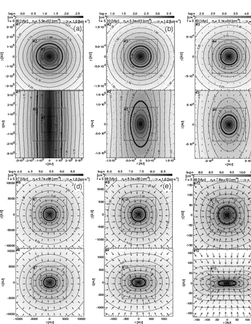
Figure 1: The density (grey-scale and contour) and velocity distributions (arrows) in model AS [($\alpha$, $\omega$, ${A_{\varphi}}$)=(0.01, 0.01, 0.01)]. Panels (a) through (f) are snapshots at the stages of (a) $n_{c}=5.5\times 10^{2}\,{\rm cm}^{-3}$ ($l=1,2$),  (b) $5.3\times 10^{3}\,{\rm cm}^{-3}$ ($l=2,3$),  (c) $5.1\times 10^{4}\,{\rm cm}^{-3}$ ($l=3,4$),  (d) $9.7\times 10^{6}\,{\rm cm}^{-3}$ ($l=6,7$),  (e) $8.3\times 10^{8}\,{\rm cm}^{-3}$($l=9,10$),  and  (f) $7.6\times 10^{10}\,{\rm cm}^{-3}$($l=12,13$), where $l$ denotes the level of subgrid. The level of the subgrid is shown in the upper left corner of each solid square which denotes the outer boundary of the subgrid. The upper and lower panels show the cross sections at $z$=0 and $y$=0 planes, respectively. The grey-scale is different for each panel as shown above the panels. Thick contours denote the density of $n=1/10\,n_{c}$, where $n_{c}$ means density at the center. The elapsed time, density at the center and arrow scale are denoted in each panel.

This subsection displays model AS as a typical model having a weak magnetic field and slow rotation. Model AS has parameters $\alpha=0.01$, $\omega=0.01$ and ${A_{\varphi}}=0.01$. Fig. 1 shows the cloud evolution in model AS by a series of cross sections.

As shown in Fig. 1, a gas cloud is transformed from a prolate one to an oblate one on the $y=0$ plane (see lower panels), while it maintains a round shape on the $z=0$ plane (upper panels) in the period of $5.5\times 10^{2}\,{\rm cm}^{-3}<n_{c}<7.6\times 10^{10}\,{\rm cm}^{-3}$. The velocity field is almost spherically symmetric while the central density increases from $5\times 10^{5}\,{\rm cm}^{-3}$ to $2\times 10^{9}\,{\rm cm}^{-3}$. The dense cloud is prolate and elongated in the $z$-direction in the lower panel of Fig. 1 (b), while it is nearly spherical in the lower panel of Fig. 1 (c). In this early collapse phase, the cloud contracts along the major axis (i.e. $z$-axis), regardless of the magnetic field and rotation as discussed in Bonnell et al. (1996). An oblate core is seen in panel Fig. 1 (e) and a thin disk is seen in the lower panel of Fig. 1 (f). The collapse is dynamical at the stages shown in Fig. 1 (c) through Fig. 1 (f). The radial infall velocity reaches $v_{r}$ = $-0.52$ km s^-1 on the $z\,=\,0$ plane in Fig. 1 (e), while the vertical infall velocity does $v_{z}\,=\,\pm 0.58$ km s^-1 on the $z$-axis. The rotation velocity is $v_{\varphi}$ = 0.047 km s^-1 at maximum and much smaller than the infall velocities. This means gas contracts spherically in this phase. The difference between the radial and vertical infall velocities is still small ($|v_{r,{\rm max}}|\,=\,0.61$ km s^-1 and $|v_{z,{\rm max}}|\,=\,0.8$ km s^-1) in Fig. 1 (f) although a high density disk is formed.

The density increase is well approximated by $\rho_{\rm c}\,=\,2.2/[4\pi G\,(t\,-\,t_{\rm f})^{2}]$ in the period of $5\times 10^{4}\,{\rm cm}^{-3}\,\leq\,n\,\leq\,10^{9}\,{\rm cm}^{-3}$ as shown by the thick solid curve in Fig. 2. The offset is taken to be $t_{\rm f}\,=\,5.96\times 10^{6}$yr so that the central density increases in proportion to the inverse square of the time in the widest span in $\log\rho_{\rm c}$, as shown in Larson (1969). Remember that the similarity solution of Larson (1969) and Penston (1969) gives $\rho_{\rm c}\,=\,1.667/[4\pi G\,(t\,-\,t_{\rm f})^{2}]$ for spherical collapse of a non-magnetized non-rotating isothermal cloud. We have checked that the density increase is well approximated by $\rho_{\rm c}\,\simeq\,1.65/[4\pi G\,(t\,-\,t_{\rm f})^{2}]$ in a non-magnetized and non-rotating cloud of our test calculation. The density increase is 15 % slower in model AS than in the similarity solution, since $(2.2/1.667)^{1/2}\,\simeq\,1.15$. This small difference is due to the rotation and magnetic field.

To evaluate the change in the core shape shown in Fig. 1, we measure the moment of inertia for the high density gas of $\rho\,\geq\,0.1\rho_{\rm c}$. We derive the major axis ($h_{l}$), minor axis ($h_{s}$), and $z$-axis ($h_{z}$) from the moment of inertia according to Matsumoto & Hanawa (1999). The oblateness is defined as $\varepsilon_{\rm ob}\,\equiv\,(h_{l}h_{s})^{1/2}/h_{z}$ and the axis ratio is defined as $\varepsilon_{\rm ar}\,=\,h_{l}/h_{s}\,-\,1$.

The oblateness is denoted by the thick solid curve as a function of time in Fig. 3 (a) and as a function of the central density in Fig. 3 (b). The oblateness is nearly constant at $\varepsilon_{\rm ob}=0.27$ in the period of $t\ \la 4\times 10^{6}$yr (or $5\times 10^{2}\,{\rm cm}^{-3}\la n_{c}\la 5\times 10^{3}\,{\rm cm}^{-3}$). It increases and reaches $\varepsilon_{\rm ob}=1$ at the stage of $n_{c}=2\times 10^{6}\,{\rm cm}^{-3}$, which is shown in the lower panel of Fig. 1 (c). The oblateness reaches $\varepsilon_{\rm ob}=2.9$, when the disk-like structure is formed at $n_{c}=7.6\times 10^{10}\,{\rm cm}^{-3}$ as shown in the lower panel of Fig. 1 (f). The increase in $\varepsilon_{\rm ob}$ is monotonic in the period of $n_{\rm c}>5\times 10^{3}\,{\rm cm}^{-3}$.

The axis ratio is denoted by the thick solid curve as a function of time in Fig. 3 (c) and as a function of the central density in Fig. 3 (d). The axis ratio decreases from $\varepsilon_{\rm ar}$ = 0.01 to $7\times 10^{-4}$ after oscillating once over the period of $t\leq 5\times 10^{6}$ yr ( or $n_{\rm c}<5\times 10^{3}\,{\rm cm}^{-3}$). It increases in proportion to $n_{\rm c}^{1/6}$ over the period of $n_{\rm c}>5\times 10^{3}\,{\rm cm}^{-3}$. The growth rate of $\varepsilon_{\rm ar}$ coincides with that of the bar mode growing in the spherical runaway collapse (Hanawa & Matsumoto 1999). The axis ratio grows up to $3.5\times 10^{-3}$ in the isothermal collapse phase as shown in Fig. 3 (d). In order to examine dependence on the axis ratio, we compare models AS and AL, of which model parameters are the same except for the amplitude of the non-axisymmetric perturbation, ${A_{\varphi}}$. The value of $\varepsilon_{\rm ar}$ is 20 times larger in model AL than in model AS at a given stage and reaches $\varepsilon_{\rm ar}=6.8\times 10^{-2}$ at $n_{\rm c}\,=\,n_{\rm cri}$. The axis ratio is proportional to ${A_{\varphi}}$. The oblateness is nearly the same in models AS and AL. The non-axisymmetric perturbation grows linearly in models AS and AL.

The magnetic flux density increases as the density increases. The left panel of Fig. 4 shows the square root of the ratio of the magnetic pressure to the gas pressure, $B_{\rm zc}/(8\pi\rho_{\rm c}c_{\rm s}^{2})^{1/2}$, as a function of $n_{\rm c}$. Note that the ordinate is normalized by the initial value. It increases in proportion to one sixth the power of the density, i.e., $B_{\rm zc}/(8\pi\rho_{\rm c}c_{\rm s}^{2})^{1/2}\propto n_{\rm c}^{1/6}$, in the period of $10^{6}\,{\rm cm}^{-3}\leq n_{\rm c}\leq 10^{9}\,{\rm cm}^{-3}$. This means that the magnetic field increases in proportion to $B_{\rm zc}\,\propto\,n_{\rm c}^{2/3}$. This increase in $B_{\rm zc}$ is consistent with the spherical collapse of the core. When the collapse is spherically symmetric, the density and magnetic field increase inversely proportional to the cubic and square of the radius, respectively, since the magnetic field is frozen in the gas. Hence, the magnetic field is proportional to two thirds the power of the density, $B_{\rm zc}\propto\rho_{\rm c}^{2/3}$.

After the central density exceeds $10^{9}\,{\rm cm}^{-3}$, the growth of the magnetic field slows down. This slowdown coincides with the change in the core shape. The core is significantly oblate in the period of $n_{\rm c}>10^{9}\,{\rm cm}^{-3}$. Remember that the magnetic field is proportional to the square root of the density ($B_{\rm zc}\propto n_{c}^{1/2}$) when a magnetized disklike gas cloud collapses (Scott & Black 1980). This is because the disk is nearly in a hydrostatic equilibrium in the $z$-direction and the isothermal disk has the relation $n\propto\Sigma^{2}$. We use the terminology, the “disk collapse”, for this radial collapse of a disklike gas cloud. In the disk collapse, the magnetic flux density increases in proportion to the surface density ($B_{\rm zc}\propto\Sigma_{\rm c}$) since the gas is frozen in a magnetic flux tube. The relations, $n_{\rm c}\propto\Sigma_{\rm c}^{2}$ and $B_{\rm zc}\propto\Sigma_{\rm c}$, yield $B_{\rm zc}\propto n_{\rm c}^{1/2}$. In the period of $n_{\rm c}>10^{9}\,{\rm cm}^{-3}$, the growth rate of the magnetic field is intermediate between those for the spherical collapse and for the disk collapse. This is consistent with the density change over the same period.

As well as the magnetic flux density, the angular velocity of the core increases as the density increases. The right panel of Fig. 4 shows the ratio of the angular velocity to the magnetic field ($\Omega_{\rm c}/B_{\rm zc}$) normalized by the initial value ($\Omega_{\rm c,0}/B_{zc,0}$) as a function of $n_{\rm c}$. The ratio is nearly constant at the initial value. This is because both the specific angular momentum ($j$) and the magnetic flux ($\Phi$) are conserved for a central magnetic flux tube. Both the angular velocity and magnetic field increase proportionally to the inverse square of the tube radius. Hence the ratio is constant in both the spherical and the disk collapse. The conservation of the specific angular momentum implies that none of the magnetic torque, gravitational torque, and $\varphi$-component of the pressure force are significant.

Since $\Omega_{\rm c}/B_{\rm zc}$ is nearly constant, the angular velocity increases in proportion to $n_{\rm c}^{2/3}$ in the period of $10^{6}\,{\rm cm}^{-3}\leq n_{\rm c}\leq 10^{9}\,{\rm cm}^{-3}$ and the growth of $\Omega_{\rm c}$ slows down in the period of $n_{\rm c}>10^{9}\,{\rm cm}^{-3}$. When measured in units of the free fall timescale, the angular velocity increases in proportion to $\Omega_{\rm c}(4\pi G\rho_{\rm c})^{-1/2}\propto n_{\rm c}^{1/6}$ in the former period. The angular velocity in units of the free fall timescale denotes the square root of the ratio of the centrifugal force to the gravitational force. The magnetic field and rotation strengthen in the same manner during the spherical collapse, since both $B_{\rm zc}(8\pi\rho_{\rm c}c_{\rm s}^{2})^{-1/2}$ and $\Omega_{\rm c}(4\pi G\rho_{\rm c})^{-1/2}$ increase in proportion to $\rho_{\rm c}^{1/6}$.

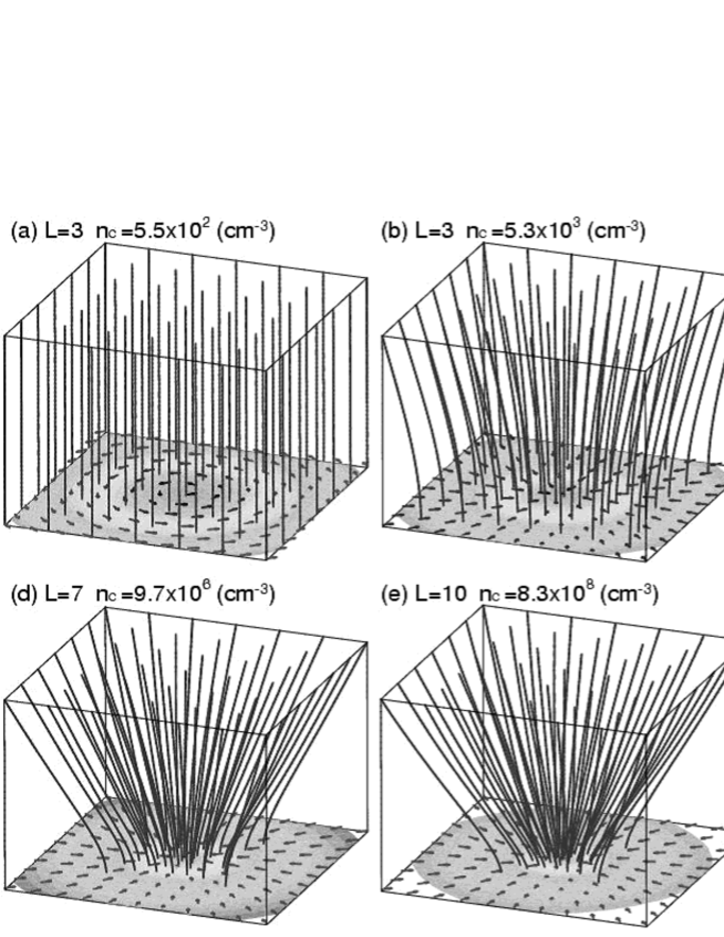
Figure 5: The magnetic field lines are shown from a bird’s eye view for model AS. Panels (a) through (f) denote the same epoch as those of Fig. 1 (a) $-$ (f), respectively. The density (gray scale) and velocity (arrows) in $z=0$ plane are also shown on the bottom. The level of subgrid and central density are shown in the upper section of each panel. Each frame denotes a cube with side lengths of (a) $1.7\times 10^{5}$ AU, (b) $1.7\times 10^{5}$ AU, (c) $8.4\times 10^{4}$ AU, (d) $1.1\times 10^{4}$ AU, (e) $1.3\times 10^{3}$ AU, and (f) $1.6\times 10^{2}$ AU, respectively.

Model AS is similar to model B of Matsumoto et al. (1997), although our model AS includes a very weak magnetic field. The magnetic field influences little the cloud collapse. Fig. 5 shows that the magnetic field is not twisted but pinched at the stages of $n_{\rm c}\,\geq\,10^{6}$ cm^-3 as shown in panels (d) - (f) of Fig. 5. Each panel denotes the magnetic field lines for the corresponding stage shown in each panel of Fig. 1. This weak magnetic field has no significant effect. When $\alpha\,<\,0.1$ and $\omega\,<0.1$, the effects of magnetic field and rotation are very small.

4.2 Strongly Magnetized and Slowly Rotating Cloud

Model BL is shown as a typical example of models in this subsection having large $\alpha$ and small $\omega$. Model BL has parameters $\alpha=0.1$, $\omega=0.01$ and ${A_{\varphi}}=0.2$. The parameters of model BL are the same as those of model AL except for $\alpha$, which is 0.01 for model AL and 0.1 for BL (Table 2). When $\alpha\,\geq\,0.1$, the magnetic pressure becomes comparable to the gas pressure in the course of cloud collapse and decelerates the radial collapse significantly. The magnetic braking is also effective in models BL and BS.

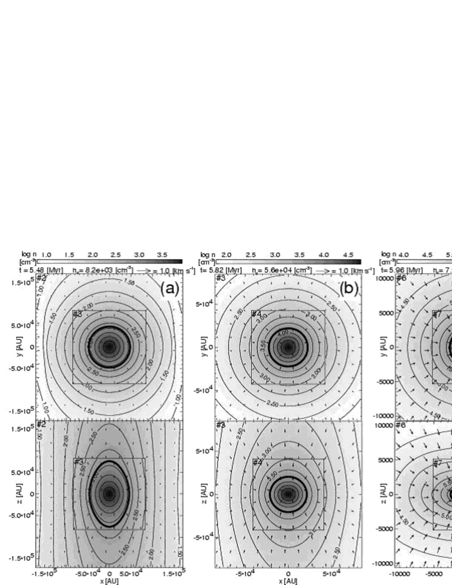
Figure 6: The density (gray scale and contours) and velocity distributions (arrows) for model BL [($\alpha$, $\omega$, ${A_{\varphi}}$)=(0.1, 0.01, 0.2)] are shown on the $z=0$ (upper panels) and $y=0$ (lower panels) planes. Panels (a) through (d) are snapshots at the stages of (a) $n_{c}=8.2\times 10^{3}\,{\rm cm}^{-3}$ ($l=2,3$),  (b) $5.6\times 10^{4}\,{\rm cm}^{-3}$ ($l=3,4$),  (c) $7.9\times 10^{6}\,{\rm cm}^{-3}$ ($l=6,7$),  and  (d) $6.0\times 10^{10}\,{\rm cm}^{-3}$ ($l=12,13$),  The contours, arrows, and notation have the same meaning as in Fig. 1.

Also in model BL the high density core changes its form from prolate to oblate as the central density increases, as shown in Fig. 6, which is the same as Fig. 1 but for model BL. The change in the core shape is due to the magnetic field, which is amplified during the spherical collapse. The ratio of the magnetic pressure to the gas pressure is 0.11 at the stage of $n_{\rm c}=2\times 10^{6}$, while it is only 0.05 at the initial stage. Each panel of Fig. 6 denotes the density and velocity distribution at the stage of (a) $n_{\rm c}\,=\,8.2\times 10^{3}\,{\rm cm}^{-3}$, (b) $5.6\times 10^{4}\,{\rm cm}^{-3}$, (c) $7.9\times 10^{6}\,{\rm cm}^{-3}$, and (d) $6.0\times 10^{10}\,{\rm cm}^{-3}$. At the stage of $n_{\rm c}\,=\,8.2\times 10^{3}\,{\rm cm}^{-3}$, the oblateness is $\varepsilon_{\rm ob}$ = 0.58 in model BL [Fig. 6(a)] while $\varepsilon_{\rm ob}$ = 0.45 in model AL [Fig. 1(b)] . The core is more oblate in model BL than in models AL and AS when compared at a given stage with the same central density [Fig. 3(b)]. The oblateness is $\varepsilon_{\rm ob}$ = 5.3 at the stage of $n_{\rm c}\,=\,5\times 10^{10}\,{\rm cm}^{-3}$ in model BL, while $\varepsilon_{\rm ob}=2.9$ in model AS (see Fig. 3). The oblateness increases slowly over the period of $3\times 10^{3}\,{\rm cm}^{-3}\la n_{\rm c}\la 10^{10}\,{\rm cm}^{-3}$ in model BL and is saturated around $\varepsilon_{\rm ob}\simeq 5$ in the period of $n_{\rm c}\ga 10^{10}\,{\rm cm}^{-3}$.

As well as in models AS and AL, the axis ratio decreases from the initial value of $\varepsilon_{\rm ar}=0.2$ to 0.015 in the period of $n_{\rm c}\,\la\,10^{4}\,{\rm cm}^{-3}$ in model BL. Then it switches to growing in proportion to $n_{\rm c}^{1/6}$ in the period of $n_{\rm c}\,\ga\,10^{4}\,{\rm cm}^{-3}$. The core is elliptic on the $x-y$ plane and the axis ratio is $\varepsilon_{\rm ar}$ = 0.23 at the stage of $n_{\rm c}\,=\,5\times 10^{10}\,{\rm cm}^{-3}$, as shown in the upper panel of Fig. 6 (d). The amplitude of the non-axisymmetic perturbation is linearly proportional to the initial amplitude. The axis ratio is always smaller by a factor of 20 in model BS than in model BL when compared at the stage of a given central density. Models BS and BL have the same model parameters except for ${A_{\varphi}}$.

Since the core is appreciably oblate, the infall velocity is higher in the vertical direction than in the radial direction. At the stage of $n_{\rm c}=5\times 10^{10}\,{\rm cm}^{-3}$ the radial infall velocity is $v_{r}=-0.46\,{\rm km}~{}{\rm s}^{-1}$ at maximum in $z\,=\,0$ plane while the vertical infall velocity is $v_{z}=0.7\,{\rm km}~{}{\rm s}^{-1}$ at maximum on the $z$-axis. The radial infall velocity is smaller and the vertical infall velocity is larger than in model AS. This asymmetry is due to the magnetic field. The rotation velocity is quite small ($v_{\varphi}=0.03\,{\rm km}~{}{\rm s}^{-1}$) and the centrifugal force is negligible. The density increase due to collapse is slower in model BL than in model AS. The growth of the central density is well approximated by $\rho_{\rm c}\,=\,2.5/[4\pi G\,(t\,-\,t_{\rm f})^{2}]$. The growth rate is 7 % smaller than that of model AS at a given central density.

Also in model BL, the magnetic field strengthens as the density increases. The ratio of the magnetic pressure to the gas pressure increases very slowly in the period of $n_{\rm c}\la 10^{6}\,{\rm cm}^{-3}$ (see Fig. 4). It is saturated around $(B_{\rm zc}/B_{\rm zc,0})^{2}/(\rho_{c}/\rho_{c,0})\simeq 1.3$ in the period of $n_{\rm c}\ga 10^{6}\,{\rm cm}^{-3}$. The magnetic field decelerates the radial collapse appreciably as shown earlier.

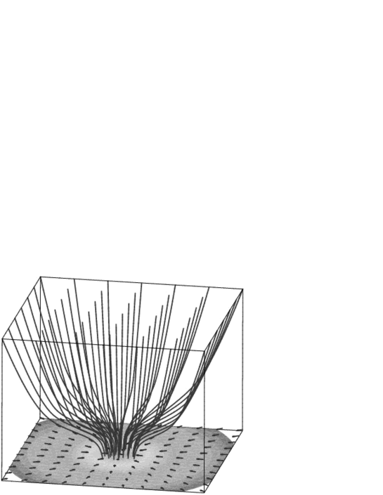
Figure 7: The magnetic field lines are shown at the same epoch of Fig. 6 (d). The level of subgrid and central density are $l=13$ and $n_{c}=6.0\times 10^{10}\,{\rm cm}^{-3}$, respectively. The frame denotes a cube with a side length of 160 AU. The gray scale and arrows have the same meaning as in Fig. 5.

Fig. 7 shows the magnetic field lines at the stage of $n_{\rm c}\,=\,6\times 10^{10}\,{\rm cm}^{-3}$. The magnetic field lines break at the levels of $z\simeq 15$ AU and 30 AU near the disk surface. The latter break corresponds to a fast-mode MHD shock, which is essentially the same as the shock waves seen in Norman, Wilson & Barton (1980), Matsumoto et al. (1997), and Nakamura et al. (1999). They are squeezed and vertical to the midplane below the shock front while they are open above the shock front. The disk formation is due to the magnetic field.

The magnetic field extracts angular momentum from the core. As shown in Fig. 4 (b), the ratio of angular velocity to the magnetic field decreases by 30 % in the period of $5\times 10^{2}\,{\rm cm}^{-3}<n_{c}\leq 5\times 10^{10}\,{\rm cm}^{-3}$ in model BL, although it remains constant in model AL. The decrease is due to the magnetic braking. The twisted magnetic field transfers the angular momentum of the core outwards. The specific angular momentum of the core is 70 % of the initial value at the stage of $n_{\rm c}=5\times 10^{10}\,{\rm cm}^{-3}$. The angular velocity normalized by free-fall timescale [$\Omega_{c}/(4\pi G\rho_{\rm c})^{1/2}$] increases slightly from 0.01 to 0.015 in the period of $5\times 10^{2}<n_{c}\leq 5\times 10^{10}\,{\rm cm}^{-3}$ in model BL, while it spins up from 0.01 to 0.06 in model AL. We discuss this difference again in §4.5 in which we compare the increase in $\Omega_{c}$ for various models.

The efficiency of the magnetic braking is qualitatively similar in models BS and BL.

Models BL and BS are similar to model C of Tomisaka (1995) and model B1 of Nakamura et al. (1999), although the earlier models include neither rotation nor non-axisymmetric perturbation. The rotation and non-axisymmetric perturbation have little effect on the cloud collapse in our models BL and BS. When the initial magnetic pressure is larger than a tenth of the gas pressure ($\alpha\geq 0.1$), initially weak magnetic field is amplified during the collapse and affects the evolution of the core. The magnetic pressure decelerates the radial collapse and leads to disk formation. Also the magnetic braking is appreciable.

4.3 Weakly Magnetized and Rapidly Rotating Cloud

This subsection describes model CS as a typical example for models having small $\alpha$ and large $\omega$. Model CS has parameters of $\alpha\,=\,0.01$, $\omega\,=\,0.5$, and ${A_{\varphi}}\,=\,0.01$. When $\omega\,\geq\,0.1$, rotation affects the collapse of the cloud significantly.

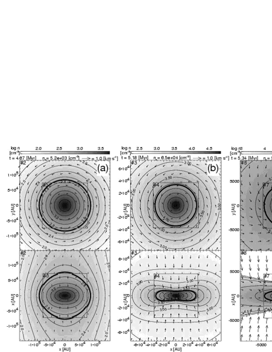
Figure 8: The density (grey scale and contours) and velocity distributions (arrows) for model CS [($\alpha$, $\omega$, ${A_{\varphi}}$)=(0.01, 0.5, 0.01)] are shown on the $z=0$ (upper panels) and $y=0$ (lower panels) planes. Panels (a) through (d) are snapshots at the stages of (a) $n_{c}=5.2\times 10^{3}\,{\rm cm}^{-3}$ ($l=2,3$),  (b) $6.5\times 10^{4}\,{\rm cm}^{-3}$ ($l=3,4$),  (c) $5.7\times 10^{6}\,{\rm cm}^{-3}$ ($l=6,7$),  and  (d) $8.3\times 10^{10}\,{\rm cm}^{-3}$ ($l=12,13$),  The contours, arrows, and notation have the same meaning as in Fig. 1.

In model CS, a rotating disk forms at an early stage of low central density. Each panel of Fig. 8 denotes the density and velocity distribution at the stages of (a) $n_{\rm c}\,=\,5.2\times 10^{3}\,{\rm cm}^{-3}$, (b) $6.5\times 10^{4}\,{\rm cm}^{-3}$, (c) $5.7\times 10^{6}\,{\rm cm}^{-3}$, and (d) $8.3\times 10^{10}\,{\rm cm}^{-3}$. The rotating disk is clearly seen at the stage of $6.5\times 10^{4}\,{\rm cm}^{-3}$. The oblateness reaches $\varepsilon_{\rm ob}=3.0$ at the stage of $4.0\times 10^{4}\,{\rm cm}^{-3}$ and is saturated around $\varepsilon_{\rm ob}\,\simeq\,3.5$ in the period of $5\times 10^{5}\,{\rm cm}^{-3}\la n_{\rm c}<5\times 10^{10}\,{\rm cm}^{-3}$ as shown in Fig. 3 (b).

The axis ratio increases up to $\varepsilon_{\rm ar}\,=\,0.2$ by the stage of $n_{\rm c}\,=\,5\times 10^{10}\,{\rm cm}^{-3}$ in model CS (see Fig. 3). At the stage of $n_{\rm c}\,=\,5\times 10^{10}\,{\rm cm}^{-3}$, the axis ratio is larger in model CS than in model AS, while it is the same at the initial stage. The difference arises in the period of $n_{\rm c}\,\leq\,5\times 10^{4}\,{\rm cm}^{-3}$. The axis ratio remains around 0.01 in model CS, while it decreases to $7\times 10^{-4}$ in model AS. The axis ratio grows roughly in proportion to $n_{\rm c}^{1/6}$ in the period of $n\,\ga\,5\times 10^{4}\,{\rm cm}^{-3}$ both in model AS and in model BS. We have confirmed that the non-axisymmetric perturbation is proportional to the initial perturbation by comparing with model CL of which initial parameters are the same as those of model CS except for ${A_{\varphi}}$. The axis ratio is 20 times larger in model CL than in model CS in the period of $n_{\rm c}\,\la\,1.0\times 10^{9}\,{\rm cm}^{-3}$. The axis ratio reaches $\varepsilon_{\rm ar}=10.2$ and the high density core has a bar shape at the stage of $n_{\rm c}\,=\,5\times 10^{10}\,{\rm cm}^{-3}$ in model CL.

The increase in the central density is approximated by $\rho_{\rm c}\,=\,6.2/[4\pi G\,(t\,-\,t_{\rm f})^{2}]$. The rate of the increase is appreciably smaller than those of models AS and BS. It is 1.93 times smaller than that of the spherical collapse at a given central density. The relatively slow collapse is due to fast rotation.

In the period of $n_{\rm c}\la 5\times 10^{5}\,{\rm cm}^{-3}$ the cloud collapses mainly in the vertical direction along the magnetic field. Accordingly the magnetic field increases a little and the ratio of the magnetic pressure to the gas pressure decreases in this period (see Fig. 4). Note that the square root of the ratio of the magnetic pressure to the gas pressure decreases in proportion to $\rho_{\rm c}^{-1/2}$ when the collapse is purely vertical along the magnetic field. Also, the angular velocity increases a little and decreases in proportion to $\rho_{\rm c}^{-1/2}$ when measured in the freefall timescale.

In the period of $5\times 10^{2}\,{\rm cm}^{-3}<n_{c}\la 5\times 10^{10}\,{\rm cm}^{-3}$, the magnetic field ($B_{\rm zc}$) strengthens and the angular velocity of the core ($\Omega_{\rm c}$) continue to increases. However, the ratio of the magnetic pressure to the gas pressure remains nearly constant around $(B_{\rm zc}/B_{\rm zc,0})^{2}/(\rho_{c}/\rho_{c,0})=0.5$ for $5\times 10^{5}\,{\rm cm}^{-3}<n_{c}\la 5\times 10^{10}\,{\rm cm}^{-3}$ as shown in Fig. 4. The angular velocity measured in the freefall timescale is also nearly constant around $\Omega_{c}(4\pi G\rho_{\rm c})^{-1/2}=0.2$. In other words, both the magnetic field and angular velocity increase in proportion to $\rho_{\rm c}^{1/2}$. These dependences of $B_{zc}$ and $\Omega_{\rm c}$ on $\rho_{\rm c}$ indicate that the core collapses in the radial direction while maintaining a disk shape. They are the same as those in the similarity solution for a self-gravitationally collapsing gas disk (Tomisaka 1995, 2002; Nakamura et al. 1995; Matsumoto et al. 1997; Saigo & Hanawa 1998).

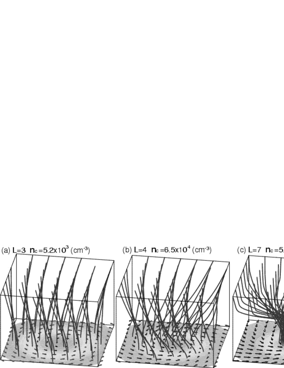
Figure 9: The magnetic field lines at the same epoch of Fig. 8. Each frame denotes a cube with side lengths of (a) $1.7\times 10^{5}$ AU, (b) $8.4\times 10^{4}$ AU, (c) $1.1\times 10^{4}$ AU, and (d) $1.6\times 10^{2}$ AU, respectively. The gray scale and arrows have the same meaning as in Fig. 5.

The ratio of the angular velocity to the magnetic field is constant in the period of $n_{\rm c}<10^{7}\,{\rm cm}^{-3}$. It increases up to 1.2 by the stage of $n_{c}=5\times 10^{10}\,{\rm cm}^{-3}$. This increase is due to the torsional Alfvén wave. The magnetic braking is not significant in model CS. The ratio of the angular velocity to the magnetic field is constant during the collapse as shown in Fig. 4 (b). This confirms that the specific angular momentum is conserved. The magnetic field is twisted by fast rotation as shown in Fig. 9. It is also bent at the shock front as well as in model BS. The twisted magnetic field is too weak to have any appreciable dynamical effects.

The infall velocity is higher vertically than radially. The maximum infall velocity is $v_{r,{\rm max}}\,=\,-0.37\,{\rm km}~{}{\rm s}^{-1}$ radially and $v_{z,{\rm max}}\,=\,\pm 0.59\,{\rm km}~{}{\rm s}^{-1}$ at the stage of $n_{c}=5\times 10^{10}\,{\rm cm}^{-3}$. The maximum rotation velocity is $v_{\varphi}=0.36\,{\rm km}~{}{\rm s}^{-1}$ and exceeds the sound speed at the same stage. Thus both the infall and rotation are supersonic. This dynamically infalling gas disk is similar to infalling envelopes observed in HL Tau (Hayashi et al., 1993) and L1551 IRS5 (Ohashi et al., 1996; Saito et al., 1996) in the sense that the radial infall velocity is comparable with the rotation velocity. The vertical inflow along the $z$-axis forms shock waves twice, once at the stage of $n_{\rm c}\,=\,5.7\times 10^{6}\,{\rm cm}^{-3}$ [see Fig. 8 (c)] and at that of $n_{\rm c}\,=\,8.3\times 10^{10}\,{\rm cm}^{-3}$ [see Fig. 8 (d)]. The former forms at $z\,=\,\pm 4\times 10^{3}$ AU, and the latter at $z\,=\pm\,40$ AU. These shock waves are essentially the same as those seen in Matsumoto et al. (1997). The oblateness has a temporal maximum value at the stages of the shock formation.

4.4 Strongly Magnetized and Rapidly Rotating Cloud

This subsection describes model DL as a typical example of models having large $\alpha$ and large $\omega$. Model DL has parameters $\alpha=1.0$, $\omega=0.5$ and ${A_{\varphi}}=0.2$. When $\alpha\geq 0.1$ and $\omega\,\geq\,0.1$, both magnetic field and rotation affect the collapse of the cloud significantly. The magnetic braking is also effective.

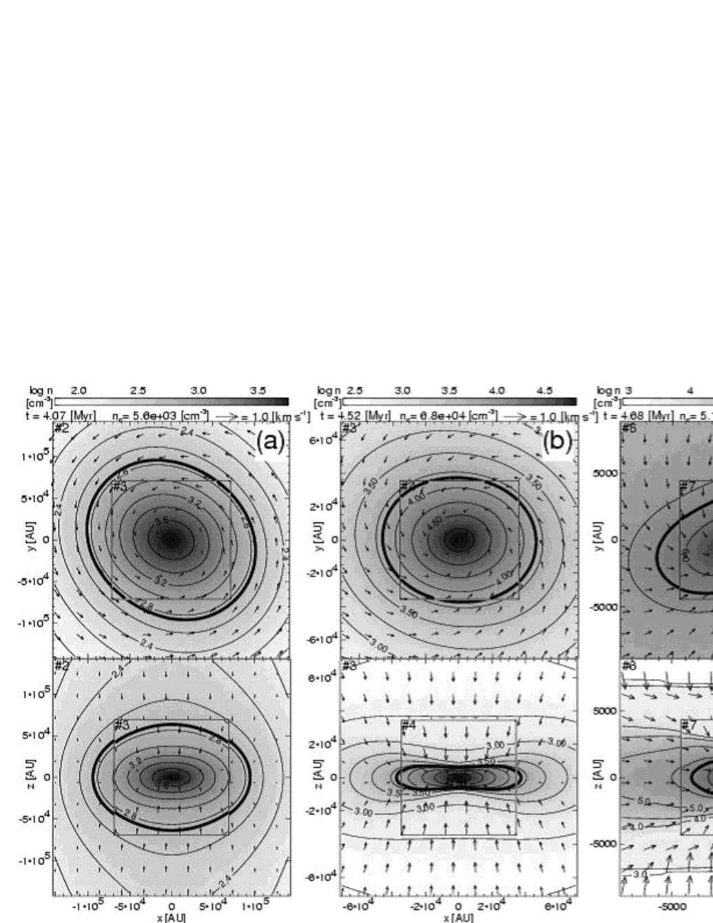
Figure 10: The density (grey scale and contours) and velocity distributions (arrows) for model DL [($\alpha$, $\omega$, ${A_{\varphi}}$)=(1, 0.5, 0.2)] are shown on the $z=0$ (upper panels) and $y=0$ (lower panels) planes. Panels (a) through (d) are snapshots at the stages of (a) $n_{c}=5.6\times 10^{3}\,{\rm cm}^{-3}$ ($l=2,3$),  (b) $6.8\times 10^{4}\,{\rm cm}^{-3}$ ($l=3,4$),  (c) $5.1\times 10^{6}\,{\rm cm}^{-3}$ ($l=6,7$),  and  (d) $5.3\times 10^{10}\,{\rm cm}^{-3}$ ($l=12,13$),  The contours, arrows, and notation have the same meaning as in Fig. 1.

Fig. 10 shows formation of a magnetized rotating disk that deforms to an elongated high density bar in model DL. Each panel denotes the density and velocity distribution at the stage of (a) $n_{\rm c}\,=\,5.6\times 10^{3}\,{\rm cm}^{-3}$, (b) $6.8\times 10^{4}\,{\rm cm}^{-3}$, (c) $5.1\times 10^{6}\,{\rm cm}^{-3}$, and (d) $5.3\times 10^{10}\,{\rm cm}^{-3}$. The high density gas has an oblateness of $\varepsilon_{\rm ob}=4.2$ at the stage of $n_{c}=6.8\times 10^{4}\,{\rm cm}^{-3}$. The oblateness reaches its maximum at $n_{\rm c}\simeq 4\times 10^{5}\,{\rm cm}^{-3}$ and oscillates around $\varepsilon_{\rm ob}\simeq 5$ in the period of $4\times 10^{5}\,{\rm cm}^{-3}\,\la\,n_{\rm c}\,\leq\,5\times 10^{10}\,{\rm cm}^{-3}$ (see Fig. 3). As a result of the strong magnetic field and fast rotation, the disk forms at an earlier stage in model DL than in the other models shown in the previous subsections.

The increase in the central density is approximated by $n_{\rm c}=4.9/|4\pi\,G\,(t-t_{\rm f})^{2}|$. This is slower than in models AS and BS, although faster than in model CS. The density increase is faster in a model having a larger $\alpha$ for a given $\omega\,\geq\,0.1$. This is because a stronger magnetic field brakes the rotating core more effectively and the centrifugal force is reduced more. Remember that the density increase is slower in a model having a larger $\alpha$, when $\omega\ll 0.1$. When the angular momentum of the cloud is very small, the centrifugal force is negligible and its reduction due to the magnetic braking is unimportant. A stronger magnetic field decelerates the collapse through higher magnetic pressure and tension. The magnetic field plays two roles: acceleration of the collapse through magnetic braking, and deceleration of the collapse through magnetic pressure and tension. The former dominates for $\omega\geq 0.1$ while the latter dominates for $\omega<0.1$.

As shown in Fig. 10 (d) upper panel, the disk is elongated into a bar of $\varepsilon_{\rm ar}=15$ at the stage of $5.3\times 10^{10}\,{\rm cm}^{-3}$. As well as in model CL, the axis ratio remains nearly constant at the beginning and increases in proportion to $n_{\rm c}^{1/6}$ from an early stage of $n_{\rm c}<5\times 10^{3}\,{\rm cm}^{-3}$ in model DL (see Fig. 3). An elongated bar forms in the models in which the non-axisymmetric perturbation is relatively large (${A_{\varphi}}>0.2$) and does not diminish in the early phase. Remember that the axis ratio decreases in the period of $n_{\rm c}\la 1.0\times 10^{4}\,{\rm cm}^{-3}$ in models AL and BL. The axis ratio increases in proportion to $n_{\rm c}^{1/6}$ in all models while the core collapses dynamically. The final axis ratio depends on the initial value and the amount of damping in the early phase. The initial damping is smaller when either the initial magnetic field or rotation is larger.

A similar bar structure is also seen in Durisen et al. (1986) and Bate (1998). The bar structure develops as a result of the bar mode instability, when the ratio of rotational to gravitational energy ($\beta$) of the core exceeds $\beta=0.274$. This $\beta$ is related to $\omega$ by $\beta=\omega^{2}$, when the cloud is spherical and has constant density and angular velocity. Thus, the criterion for the ‘bar mode instability’, $\beta>0.274$, corresponds to $\omega>0.523$. The value of $\omega$ continues to decrease until it converges to $\omega\simeq 0.2$ as denoted in the following subsection. Therefore, the condition $\omega>0.523$ is never fulfilled, and the bar should form in model D by another mechanism. While the bar mode instability of Hanawa & Matsumoto (1999) works only in a dynamically collapsing cloud, the bar mode instability of Durisen et al. (1986) and Bate (1998) does in a cloud in hydrostatic equilibrium.

There is another evidence that the bar is formed not by fast rotation in our models. The bar forms also in the model of ($\alpha$, $\omega$, ${A_{\varphi}}$) = (3, 0, 0.2), which is listed as model 56 in Table 2 of Paper II. The bar formation can not be due to rotation since the cloud does not rotate in this model. (See Table 2 of Paper II for the list of the models in which the bar forms at the end of the isothermal phase.)

As well as in models CS and CL, the vertical infall dominates over the radial infall in the period of $n_{\rm c}\la 7\times 10^{4}\,{\rm cm}^{-3}$ in models DS and DL. The ratio of the magnetic pressure to the gas pressure normalized by its initial value decreases to 0.5 in the period as shown in Fig. 4. Then it oscillates around 0.5 in the period of $10^{5}\la n_{c}\la 5\times 10^{10}\,{\rm cm}^{-3}$. The epoch of disk formation coincides with that at which the ratio of the magnetic pressure to the gas pressure reaches its first local minimum value.

The vertical inflow also forms shock waves twice in model DL. Fig. 10(c) shows the outer shock located at $z=\pm 7000$ AU. The flow is nearly vertical above the front while it is horizontal below. The epoch of shock formation coincides with that of the temporarily maximum oblateness as in model CL.

The magnetic braking slows the spin of the collapsing disk in model DL. The initial central angular velocity is $\Omega_{c}/(4\pi G\rho_{\rm c})^{1/2}=0.5$ in both models CL and DL. The central angular velocity decreases to $\Omega_{c}/(4\pi G\rho_{\rm c})^{1/2}=0.21$ by the stage of $n_{\rm c}\,=\,5\times 10^{4}\,{\rm cm}^{-3}$ in model DL, while it decrease to 0.24 in model CL. The ratio of the angular velocity to the magnetic field ($\Omega_{c}/B_{zc}$) normalized by the initial value ($\Omega_{\rm c,0}/B_{\rm zc,0}$) decreases to 70 % of the initial value in model DL (see Fig. 4). The magnetic braking is effective in the period of $n_{\rm c}\leq 7\times 10^{5}\,{\rm cm}^{-3}$ as in model BL. The ratio of the angular velocity to the magnetic field increases in the period of $7\times 10^{5}\,{\rm cm}^{-3}<n_{\rm c}<5\times 10^{8}\,{\rm cm}^{-3}$. This spin is due to the magnetic torque. The twist of the magnetic field is bounded by the shock front and the torsional Alfvén wave is reflected there. Thus the angular momentum is not released from the core in model DL.

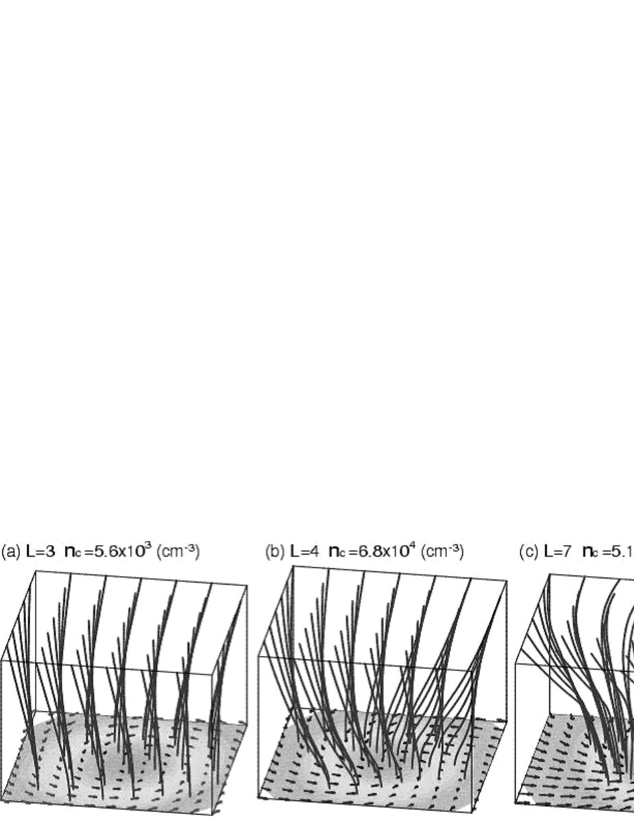
Figure 11: The magnetic field lines at the same epoch of Fig. 10. Each frame denotes a cube with side lengths of (a) $1.7\times 10^{5}$ AU, (b) $8.4\times 10^{4}$ AU, (c) $1.1\times 10^{4}$ AU, and (d) $1.6\times 10^{2}$ AU, respectively. The gray scale and arrows have the same meaning as in Fig. 5.

The ratio of the magnetic pressure to gas pressure decreases from 0.5 to 0.1 in the period of $5\times 10^{2}\,{\rm cm}^{-3}\leq n_{\rm c}\la 7\times 10^{5}\,{\rm cm}^{-3}$, and remains around 0.1 in the period of $n_{\rm c}\ga 7\times 10^{5}\,{\rm cm}^{-3}$. Thus, importance of the magnetic force relative to the centrifugal force decreases in models DS and DL. Fig. 11 illustrates the magnetic field for the stages shown in Fig. 10. The magnetic field lines are twisted but less pinched than in model CS. They are twisted at a higher $z$ in model DL than in model CS. As shown in Fig. 11 (d), the magnetic field is squeezed to stem vertically from the bar and the magnetic flux density is large in the bar. In Fig. 11 (d), magnetic field lines are bent at $z\simeq 40$AU, which corresponds to the shock front. Inside the shock front, the magnetic field lines are ran vertically and hardly twisted, while twisted moderately outside of the shock front.

Models DL and DS have the same initial model parameters except for ${A_{\varphi}}$, which is smaller by a factor of 20 in model DS. As a result, only the axis ratio differs appreciably between models DL and DS. A high density disk is seen at the stage of $n_{\rm c}=5\times 10^{10}\,{\rm cm}^{-3}$ in model DS while the elongated bar is seen in model DL. The axis ratio is smaller by a factor 20 in model DL throughout the evolution.

4.5 Magnetic Flux - Spin Relation

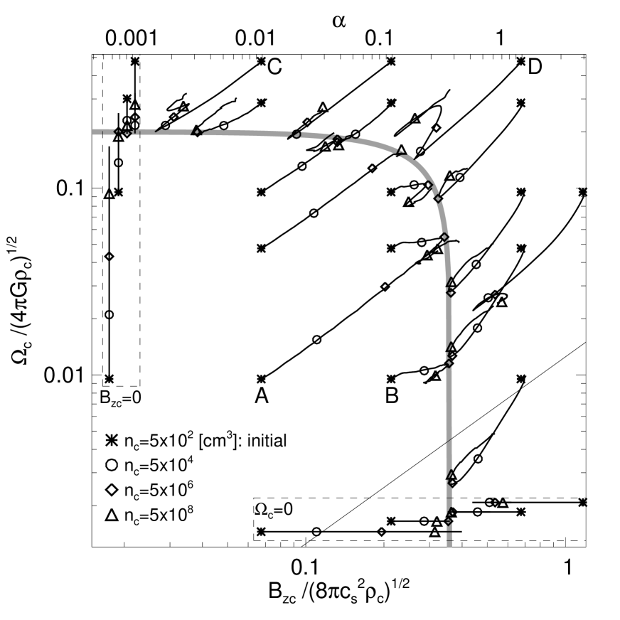
Figure 12: The evolutions of the magnetic flux density and angular velocity at cloud center. The lower axis indicates the square root of the magnetic pressure ($B_{\rm zc}/\sqrt{8\pi}$) normalized by the square root of the thermal pressure ($\sqrt{c_{s}^{2}\rho_{c}}$) and the left ordinate does the angular speed ($\Omega_{c}$) normalized by the freefall timescale ($\sqrt{4\pi G\rho_{c}}$), respectively. The upper axis indicates the parameter, $\alpha$. The symbols, $*$, $\circ$, $\diamond$, and $\triangle$, represent at $n_{c}=5\times 10^{2}\,{\rm cm}^{-3}$ (initial state), $5\times 10^{4}\,{\rm cm}^{-3}$, $5\times 10^{6}\,{\rm cm}^{-3}$, and $5\times 10^{8}\,{\rm cm}^{-3}$, respectively. Each line denotes the evolutional path from the initial state ($n_{\rm c,0}=5\times 10^{2}\,{\rm cm}^{-3}$) to the end of the isothermal phase ($n_{\rm c}=5\times 10^{10}\,{\rm cm}^{-3}$). The characters ’A’, ’B’, ’C’ and ’D’ denote the model shown in Table 1. The thick curve denotes the magnetic flux and spin relation, $\Omega^{2}/[(0.2)^{2}\times 4\pi G\rho_{c}]+B_{zc}^{2}/[(0.36)^{2}\times 8\pi c_{s}^{2}\rho_{c}]=1$ [see Equation (19)]. The thin line indicates the relation of $\Omega_{\rm c}/(4\pi G\rho_{\rm c})^{1/2}\propto B_{\rm zc}/(8\pi c_{s}^{2}\rho_{\rm c})^{1/2}$. The models with no magnetic field are shown inside the upper left box, while those with no rotation are shown inside the lower right box.

The filamentary cloud fragments to form a high density core of $n_{\rm c}>5\times 10^{10}$ in all the models computed. The formation of the core is dynamical and the central density increases in proportion to the inverse square of the time. As the central density increases, the magnetic field increases roughly in proportion to a power of $\rho_{\rm c}$. The power index, however, differs and depends on the geometry of the collapse as shown in the previous subsections. Also the angular velocity increases in proportion to a power of $\rho$ and the power index depends on the geometry of the collapse and the strength of the magnetic field. To summarize the increase in $B_{\rm zc}$ and $\Omega_{c}$ we have plotted the evolutionary locus of the core in Fig. 12. The abscissa denotes the square root of the ratio of the magnetic pressure to the gas pressure, $B_{\rm zc}(8\pi c_{\rm s}^{2}\rho_{\rm c})^{-1/2}$, in the logarithmic scale. The ordinate denotes the angular velocity normalized by the freefall timescale, $\Omega_{c}(4\pi G\rho_{\rm c})^{-1/2}$, on the logarithmic scale. Each curve denotes the evolutionary locus for a model. The asterisks denote the initial stages. The circles, squares and triangles denote the stages of $n_{\rm c}=5\times 10^{4}\,{\rm cm}^{-3}$, $5\times 10^{6}\,{\rm cm}^{-3}$, and $5\times 10^{8}\,{\rm cm}^{-3}$, respectively. Models without magnetic field are shown inside the upper left box. Models without rotation are shown inside the lower right box.

The evolutionary loci are systematically ordered in Fig. 12. They are aligned to evolve toward the upper right in the lower left region. Models AL and AS belong to this region of weak magnetic field and slow rotation. On the other hand, the loci are aligned to evolve toward the lower left in the upper region (fast rotation) and in the right region (strong magnetic field). Models CL, CS, DL, and DS belong to these regions. Models BL and BS appear in the middle of the panel. Their loci are nearly horizontal and the angular velocity measured on the freefall timescale does not increase as a result of the magnetic braking.

We can deduce several rules for the collapse of a magnetized rotating gas cloud from Fig. 12. First all the loci seem to converge on the curve,

$${\displaystyle\frac{\Omega_{c}^{2}}{(0.2)^{2}\;4\pi G\rho_{\rm c}}}+{\displaystyle\frac{B_{\rm zc}^{2}}{(0.36)^{2}\;8\pi c_{s}^{2}\rho_{c}}}=1.$$ (19)

Equation (19) is denoted by the thick solid curve in Fig. 12. We call this curve the magnetic flux - spin relation or $B-\Omega$ relation in the following. The first term of equation (19) is proportional to the square of the angular velocity normalized by the freefall timescale and accordingly is proportional to the ratio of the centrifugal force to the gravity. The second term is proportional to the ratio of the magnetic pressure to the gas pressure. The numerators are proportional to the anisotropic forces which suppress only the radial infall. Convergence to equation (19) indicates that the sum of the centrifugal and magnetic forces are regulated to be at a certain value. This rule involves the rules found by Matsumoto et al. (1997) and Nakamura et al. (1999) as a special case. The former showed that the ratio of the specific angular momentum to the core mass converges to a half of the critical value $j=0.5(2\pi GM/c_{\rm s})$ for models having no magnetic field. The latter showed that the ratio of the magnetic field to the surface density tends to be a half of the critical one, i.e., $B_{\rm zc}=0.5(2\pi G)^{1/2}\Sigma$, for collapse of a non-rotating cloud. See the models shown inside the upper left box and those inside the lower right box to confirm that they also converge to equation (19).

The magnetic flux - spin relation is related to formation of the shock waves. The first shock wave forms exactly when the evolutionary locus reaches the $B-\Omega$ relation. After the shock formation, the evolutionary locus leaves it temporarily and reaches it again at the formation of the second shock wave. The shock strength is also related to the distance between the initial stage and the $B-\Omega$ relation on the $B-\Omega$ diagram. The shock wave is stronger in a model starting from a more distant place from equation (19) on the diagram. No shock wave forms in a model of which the initial stage is close to equation (19) on the diagram (see, e.g., the model of $\alpha=0.1$ and $\omega=0.1$ shown in Fig. 12).

Second, the magnetic braking is appreciable only in models having $\alpha\simeq 0.1$. The effect of the magnetic braking is evaluated from the slope on the diagram, $d\log\Omega_{\rm c}/d\log B_{\rm zc}$. When the specific angular momentum is conserved, the slope is $d\log\Omega_{\rm c}/d\log B_{\rm zc}=1$ as discussed in subsection 4.3. The slope differs appreciably from unity near the lower part of the $B-\Omega$ relation in Fig. 12. It is appreciably smaller than unity on the left-hand side of the $B-\Omega$ relation, while it is appreciably larger on the right-hand side. When the initial magnetic field is very weak, its magnetic torque is negligible. When the initial magnetic field is strong, the vertical collapse dominates. The magnetic braking reduces the specific angular momentum by $30-40\%$ by the stage of $n_{c}\,=\,10^{6}\,{\rm cm}^{-3}$. However, it does not operate effectively beyond the stage. We will discuss the implication of equation (19) in the next section.

5 Discussion

As shown in the previous section, the magnetic flux density and angular velocity converge on equation (19) in Fig. 12, the $B-\Omega$ diagram. Thus, we can evaluate the magnetic flux density and angular velocity of the first core to be

$$\left({\displaystyle\frac{\Omega_{c}}{2.57\times 10^{-3}\,{\rm yr}^{-1}}}\right)^{2}+\left({\displaystyle\frac{B_{\rm zc}}{1.50\times 10^{4}\,\mu{\rm G}}}\right)^{2}=1,$$ (20)

by substituting $\rho_{\rm c}\,=\,1.92\times 10^{-13}$ g$\,{\rm cm}^{-3}$ (equivalent to $n_{\rm c}=5\times 10^{10}\,{\rm cm}^{-3}$) and $c_{\rm s}\,=\,0.19~{}{\rm km}~{}{\rm s}^{-1}$, into equation (19). equation (20) implies that the first core has either the ‘standard’ magnetic flux density (15 mG) or the ‘standard’ angular velocity ($2.57\times 10^{-3}$ yr^-1), unless the initial magnetic field is very weak and the rotation is very slow. When both the magnetic flux density and angular velocity are negligible, the cloud collapses almost spherically and hence both $B_{\rm zc}$ and $\Omega_{\rm c}$ increase in proportion to $n_{\rm c}^{2/3}$. Thus, either the magnetic flux density or the angular velocity reach the standard value at $n_{\rm c}=5\times 10^{10}\,{\rm cm}^{-3}$ when either $B\geq 1.50~{}\mu{\rm G}$ or $\Omega_{\rm c}\geq 2.57\times 10^{-7}~{}{\rm yr}^{-1}$ at the stage of $n_{\rm c}\,=\,5\times 10^{4}\,{\rm cm}^{-3}$. The latter condition is equivalent to $|\mbox{\boldmath{$\nabla$}}\times\mbox{\boldmath$v$}|\,\geq\,2.49\times 10^{3}~{}{\rm km}~{}{\rm s}^{-1}~{}{\rm pc}^{-1}$.

The standard magnetic flux density is approximately a half of the critical one, as mentioned in subsection 4.4. The latter is evaluated to be

$$B_{\rm cr} = 2\pi\sqrt{G}\Sigma$$ (21)

$$= \sqrt{8\pi\rho c_{\rm s}^{2}}$$ (22)

at the limit of the geometrically thin self-gravitationally bound gas disk (Nakano & Nakamura, 1978). Also, the standard angular velocity is approximately a half of the critical one. The critical angular velocity is defined so that the centrifugal force balances with the gravity. Then it is evaluated to be

$$\Omega_{\rm cr}\,=\,\sqrt{{\displaystyle\frac{4\pi G\rho}{3}}}$$ (23)

for a uniform gas sphere. Thus, equation (19) implies that either the magnetic flux density or the angular velocity is regulated to be a half of the critical value.

Equation (19) also predicts anti-correlation between the magnetic flux density and angular velocity of the first core. In other words, only one of the magnetic flux density or the angular velocity is close to the standard value. Then we can make a new index, the ratio of angular velocity to the magnetic flux density, for identifying whether the magnetic field dominates over rotation during the cloud collapse. If it is larger than the ratio of the standard values,

$${\displaystyle\frac{\Omega_{\rm st}}{B_{\rm st}}} = 0.39\,\sqrt{G}{c_{\rm s}}^{-1}$$ (24)

$$= 1.69\times 10^{-7}\,\left(\frac{c_{\rm s}}{0.19~{}{\rm km~{}s}^{-1}}\right)^{-1}\,{\rm yr}^{-1}\,\mu{\rm G}^{-1},$$ (25)

the centrifugal force dominates over the magnetic force. Otherwise the magnetic force dominates over the centrifugal force. This analysis suggests that there exist two types of first core: magnetic first core and spinning first core. We discuss the difference between them in Paper II.

We shall apply the above discussion to L1544, the prestellar core, of which rotation and magnetic field have been measured. The rotation velocity is evaluated to be $0.09~{}{\rm km~{}s}^{-1}$ at $r$ = 15000 AU by Ohashi et al. (1999) and $0.14~{}{\rm km~{}s}^{-1}$ at $r$ = 7000 AU by Williams et al. (1999). These velocity gradients correspond to $1.26\times 10^{-6}$ yr^-1 and $4.21\times 10^{-6}$ yr^-1. On the other hand, the line-of-sight magnetic field is evaluated to be $+11\pm 2\,\mu{\rm G}$ by Crutcher & Troland (2000). Combining these values, we obtain $\Omega/B$ = $1.1\times 10^{-7}$ yr^-1 $\mu{\rm G}^{-1}$ and $3.8\times 10^{-7}$ yr^-1 $\mu{\rm G}^{-1}$. If we take account of uncertainty of the observed values, the magnetic force dominates over the centrifugal force only marginally.

It should be noted that Crutcher et al. (2004) derived a much stronger magnetic field ($\approx 140~{}\mu$G) for L1544 from linear polarization of the dust emission. They derived the value under the assumption that the randomness of the magnetic field can be ascribed to turbulent motion. If the magnetic field is as strong as 140 $\mu$G at the distance of 10000 AU, the magnetic force should dominate over the centrifugal force. However, their method gives a magnetic field an order of magnitude stronger compared with the values derived by the Zeeman effect. Possible systematic errors should be examined.

Next, we discuss the speed of dynamical collapse in the molecular cloud core. Aikawa et al. (2001) discussed the possibility of deriving the collapse speed from the chemical abundance in the prestellar core L1544. They computed chemical evolution in a molecular cloud core, assuming that the density evolution is the same as that of the Larson-Penston similarity solution, or by a factor $f$ slower. They concluded that the observed chemical anomaly in L1544 is consistent with the model based on the Larson-Penston similarity solution from comparison with the slow collapse models of $f$ = 3 and 10. The model of $f$ = 3 is supposed to mimic a molecular cloud core of which collapse is slowed down owing to rotation, magnetic field, or turbulence. Our simulation has shown that the slowing by magnetic field and rotation is appreciably smaller. The slow-down factor is evaluated to be $f$ = 1.22 for model BS and 1.93 for model CL. The small slow-down factor makes the chemical diagnosis harder.

Finally, we discuss the effect of the ambipolar diffusion. The evolution of magnetically subcritical cloud including the ambipolar diffusion has been investigated by Basu & Mouschovious (1994, 1995a, 1995b) under the disk approximation. They showed that the magnetically supercritical core is formed in the subcritical cloud for ambipolar diffusion after 10-20 freefall time passed. Once the supercritical core is formed, the magnetic field is hardly extracted from the core, because the ambipolar diffusion is much slower than the freefall (Basu & Mouschovias, 1994). Thus, our ideal MHD approximation is valid since our model cloud is supercritical from the initial stage (see Table 2). The ambipolar diffusion may have an important role in the initially subcritical cloud and after the formation of the dense core ($n_{c}>10^{11}\,{\rm cm}^{-3}$).

Table 1: Model Parameters

parameter	values
$\alpha$	0,  10-3,  5$\times$10-3,  0.01,  0.05,  0.1,  0.5,  1,  2,  3
$\omega$	0,  0.01,  0.02,  0.03,  0.04,  0.05,  0.1,  0.2,  0.3,  0.4,  0.5,  0.6
${A_{\varphi}}$	10-3,  0.01,  0.1,  0.2,  0.3
$n_{\rm c,0}$	$5\times 10^{2}\,{\rm cm}^{-3}$,  $5\times 10^{4}\,{\rm cm}^{-3}$,  $5\times 10^{6}\,{\rm cm}^{-3}$

Table 2: Parameters and Initial Conditions for Typical Models

Model		$\alpha$	$\omega$	${A_{z}}$	${A_{\varphi}}$	$n_{\rm c,0}$	$B_{\rm zc,0}$ ($\mu$G)	$\Omega_{\rm c,0}$ ($10^{8}$ yr-1)	$M$ ($\thinspace M_{\odot}$)	L ($10^{5}$ AU)	$t_{\rm f}$ (106 yr)	$M/M_{\rm B,cri}$
	AS	0.01	0.01	0.1	0.01	$5\times 10^{2}$	0.295	1.26	12.2	6.92	5.96	13.2
A	AL	0.01	0.01	0.1	0.2	$5\times 10^{2}$	0.295	1.26	12.2	6.92	5.99	13.2
	BS	0.1	0.01	0.1	0.01	$5\times 10^{2}$	0.931	1.26	12.5	6.82	5.92	4.2
B	BL	0.1	0.01	0.1	0.2	$5\times 10^{2}$	0.931	1.26	12.5	6.82	5.95	4.2
	CS	0.01	0.5	0.1	0.01	$5\times 10^{2}$	0.295	63.1	20.6	5.94	5.35	14.4
C	CL	0.01	0.5	0.1	0.2	$5\times 10^{2}$	0.295	63.1	20.6	5.94	5.38	14.4
	DS	1	0.5	0.1	0.01	$5\times 10^{2}$	2.95	63.1	28.7	5.71	4.69	1.4
D	DL	1	0.5	0.1	0.2	$5\times 10^{2}$	2.95	63.1	28.7	5.71	4.69	1.4

Figure 2: The central densities are shown as a function of time for models AS, BL, CS, and DL. The value of $t_{\rm f}$ is shown in Table 2. See text for the definition of $t_{\rm f}$. The relation of $n_{c}\propto(t-t_{\rm f})^{-2}$ is also plotted for comparison.

Figure 3: The oblateness (upper panels) and axis ratio (lower panels) are plotted against the elapsed time (left panels) and central density (right panels) for models AS, AL, BS, BL, CS, CL, DS and DL. The relation of $\varepsilon_{\rm ar}\propto n_{c}^{1/6}$ is also plotted in panel (d) for comparison.

Figure 4: The square root of the ratio of the magnetic pressure to the gas pressure normalized by the initial value, $(B_{\rm zc}/B_{\rm zc,0})/(n_{c}/n_{\rm c,0})^{1/2}$, is plotted against the central density, $n_{c}$, in the left panel. The ratio of the angular velocity to the magnetic flux density normalized by the initial value, ($\Omega_{c}/\Omega_{c,0})/(B_{\rm zc}/B_{\rm zc,0}$), is plotted against the central density in the right panel. The relation $(n_{\rm c}/n_{c,0})^{1/6}$ is also plotted in the left panel.

References

- Aikawa et al. (2001) Aikawa Y., Ohashi N., Inutsuka S., Herbst, E., Takakuwa, S., 2001, ApJ, 552, 639
- Basu & Mouschovias (1994) Basu S., Moushovias T. Ch., 1994, ApJ, 432, 720
- Basu & Mouschovias (1995a) Basu S., Moushovias T. Ch., 1995a, ApJ, 452, 386
- Basu & Mouschovias (1995b) Basu S., Moushovias T. Ch., 1995b, ApJ, 453, 271
- Bate (1998) Bate M., 1998, ApJ, 508, L95
- Bonnell & Bate (1994) Bonnell I., Bate M. R., 1994, MNRAS, 269, L45
- Bonnell et al. (1996) Bonnell I.A., Bate M.R., Price N.M., 1996, MNRAS, 279, 121
- Boss (2002) Boss A. P., 2002, ApJ, 568, 743
- Crutcher et al. (2004) Crutcher R. M., Nutter D. J., Ward-Thompson D., 2004, ApJ, 600, 279
- Crutcher & Troland (2000) Crutcher R. M., Troland T. H., 2000, ApJ, 537, L139
- Dedner et al. (2002) Dedner A., Kemm F., Kröner D., Munz C.-D., Schnitzer T., & Wesenberg M., 2002, Journal of Computational Physics, 175, 645
- Dorfi (1982) Dorfi E., 1982, A&A, 114, 151
- Dorfi (1989) Dorfi E., 1989, A&A, 225, 507
- Durisen et al. (1986) Durisen R.H., Gingold R.A., Tohline J.E., Boss A.P., 1986, ApJ, 305, 281
- Fukuda & Hanawa (1999) Fukuda F., Hanawa T., 1999, ApJ, 517, 226
- Hanawa & Matsumoto (1999) Hanawa, T., Matsumoto, T. 1999, ApJ, 521, 703
- Hayashi et al. (1993) Hayashi M., Ohashi N., Miyama S. M., 1993, ApJ, 418, L71
- Hirsh (1990) Hirsh C. 1990, Numerical Computation of Internal and External Flows, Vol. 2 (Chichester: Wiley)
- Hosking & Whitworth (2004) Hosking J. G., Whitworth A. P., 2004, 347, 1001
- Larson (1969) Larson R. B., 1969, MNRAS, 145, 271
- Li & Nakamura (2002) Li Z.-Y., Nakamura F., 2002., ApJ, 583, L256
- Machida, Tomisaka & Matsumoto (2004a) Machida M. N., Tomisaka K., Matsumoto T. 2004, MNRAS, 348, L1
- Machida, Matsumoto, Hanawa & Tomisaka (2004c) Machida M. N., Matsumoto T., Hanawa T., Tomisaka K. 2004, MNRAS, submitted (Paper II)
- Masunaga & Inutsuka (2000) Masunaga H., Inutsuka S., 2000, ApJ, 531, 350
- Matsumoto et al. (1994) Matsumoto T., Nakamura F., Hanawa T., 1994, PASJ, 46, 243
- Matsumoto et al. (1997) Matsumoto T., Hanawa T., Nakamura F. 1997, ApJ, 478, 569
- Matsumoto & Hanawa (1999) Matsumoto T., Hanawa T., 1999, ApJ, 521, 659.
- Matsumoto & Hanawa (2003a) Matsumoto T., Hanawa T., 2003a, ApJ, 583, 296
- Matsumoto & Hanawa (2003b) Matsumoto T., Hanawa T., 2003b, ApJ, 595, 913
- Matsumoto &Tomisaka (2004) Matsumoto T., Tomisaka K., 2004, ApJ, 616, 266
- Nakamura et al. (1995) Nakamura F., Hanawa T., Nakano T., 1995, ApJ, 444, 770
- Nakamura & Hanawa (1997) Nakamura F., Hanawa T., 1997, ApJ, 480, 701
- Nakamura et al. (1999) Nakamura F., Matsumoto T., Hanawa T., Tomisaka K. 1999, ApJ, 510, 274
- Nakamura & Li (2002) Nakamura F., Li Z.-Y., 2002, ApJ, 566, L101
- Nakamura & Li (2003) Nakamura F., Li Z.-Y., 2003, ApJ, 594, 363
- Nakano & Nakamura (1978) Nakano T., Nakamura T., 1978, PASJ, 30, 671
- Nakano (1988) Nakano T. 1988, PASJ, 40, 593
- Nakano, Nishi & Umebayashi (2002) Nakano T., Nishi R., & Umebayashi T. 2002, ApJ, 573, 199
- Norman, Wilson & Barton (1980) Norman M. L., Wilson J. R., Barton R. T., 1980, ApJ, 239, 968
- Ohashi et al. (1996) Ohashi N., Hayashi M., Ho P. T. P., Momose M., Hirano N. 1996, ApJ, 466, 957
- Ohashi et al. (1999) Ohashi N., Lee S. W., Wilner D. J., Hayashi M., 1999, ApJ, 518, L41
- Penston (1969) Penston M. V. 1969, MNRAS, 144, 425
- Phillips & Monaghan (1985) Phillips G. J., Monaghan J. J., 1985, MNRAS, 216, 883
- Saigo & Hanawa (1999) Saigo K., Hanawa T. 1998, ApJ, 493, 342
- Saito et al. (1996) Saito M., Kawabe R., Kitamura Y., Sunada K., 1996, ApJ, 473, 464
- Scotto & Black (1980) Scott E. H., Black D. C. 1980, ApJ, 239, 166
- Simon et al. (1992) Simon M, Chen WP, Howell RR, Slovik D. 1992, ApJ, 384, 212
- Stodółkiewicz (1963) Stodółkiewicz J. S., 1963, Acta Astron., 13, 30
- Tomisaka (1995) Tomisaka K., 1995, ApJ, 438, 226
- Tomisaka (1998) Tomisaka K., 1998, ApJ, 502, L163
- Tomisaka (2000) Tomisaka K., 2000, ApJ, 528, L41
- Tomisaka (2002) Tomisaka K., 2002, ApJ, 575, 306
- Truelove et al. (1997) Truelove J, K., Klein R. I., McKee C. F., Holliman J. H., Howell L. H., Greenough J. A., 1997, ApJ, 489, L179
- Williams et al. (1999) Williams J. P., Myers P. C., Wilner D. J., Francesco J. D., 1999, ApJ, 513, L61