Hard X-ray diffuse emission from the Galactic Center seen by INTEGRAL.

We study the hard X-ray (20-100 keV) variability of the Galactic Center (GC) and of the nearby sources on the time scale of 1000 s. We find that 3 of the 6 hard X-ray sources detected by INTEGRAL within the central $1^{\circ}$ of the Galaxy are not variable on this time scale: the GC itself (the source IGR J1745.6-2901) as well as the source 1E 1743.1-2843 and the molecular cloud Sgr B2. We put an upper limit of $5\times 10^{-12}$ erg/(cm² sec) (in 20 to 60 keV band) on the variable emission form the supermassive black hole (the source Sgr A*) which powers the activity of the GC (although we can not exclude the possibility of rare stronger flares). The non-variable 20-100 keV emission from the GC turns out to be the high-energy non-thermal tail of the diffuse hard “8 keV” component of emission from Sgr A region. Combining the XMM-Newton and INTEGRAL data we find that the size of the extended hard X-ray emission region is about $20$ pc. The only physical mechanism of production of diffuse non-thermal hard X-ray flux, which does not contradict the multi-wavelength data on the GC, is the synchrotron emission from electrons of energies 10-100 TeV.

1 Introduction

Recent observations of the Galactic Center (GC) in 1–10 keV (Baganoff et al. (2001)), 20-100 keV (Bélanger et al. (2004)), 10 MeV–10 GeV (Mayer-Hasselwander et al. (1998)) and 1–10 TeV (Aharonian et al. (2004)) reveal the high-energy activity of the nucleus of the Milky Way. This activity is powered by a supermassive black hole (BH) of mass $M_{BH}\simeq 3\times 10^{6}M_{\odot}$ (Genzel et al. (2000); Ghez et al. (2000); Schödel et al. (2002)) and has a number of puzzling properties such as an extremely low luminosity, $L_{BH}\simeq 10^{36}$ erg/s (eight orders of magnitude less than the Eddington luminosity). A number of theoretical models of supermassive BHs accreting at low rates were put forward to explain the data (Narayan et al. (2002); Melia and Falcke (2001); Aharonian and Neronov (2005)) but the “broad-band” picture of activity of the GC is still missing.

Emission from the GC has two major contributions. The first one is the variable emission from the direct vicinity of the central BH (the source Sgr A*) detected in X-rays (Baganoff et al. (2001); Porquet et al. (2003); Goldwurm et al. (2003)) and in the infrared (Genzel et al. (2003)). The typical variability time scales $T\sim 1$ ksec are close to the light-crossing time of a compact region of the size of about ten gravitational radii of the central supermassive BH, $R\sim 10R_{grav}\simeq 10^{13}$ cm. Apart from the highly variable emission from a compact object, there is a strong diffuse component which extends over tens of parsecs around the compact source. This diffuse X-ray emission has complex spatial and spectral properties (Muno et al. (2004)). In particular, it contains an extended “hard” component which is tentatively explained by the presence of hot plasma with temperature $T\simeq 8$ keV in the emission region. However, such an explanation faces serious problems because it is difficult to find objects which would produce such a hot plasma and, moreover, this plasma would not be gravitationally bound in the GC. The origin of the hard component of diffuse X-ray emission can be clarified using the data on diffuse emission in higher energy bands (above 10 keV). If the hard diffuse emission is really of thermal origin, one expects to see a sharp cut-off in the spectrum above 10 keV.

The GC was recently detected in the 20-100 keV energy band by the INTEGRAL satellite (Bélanger et al. (2004)). The source IGR J1745.6-2901 is found to be coincident with Sgr A* to within $\sim 1$ arcmin. However, the wide point spread function of ISGRI imager on board of INTEGRAL encircles the whole region of size $\sim 20$ pc around the BH which does not allow to separate the contributions of Sgr A* itself and of the possible extended emission around Sgr A*. The only possibility of separation of the two contributions is to study the time variability of the signal. Indeed, one expects to see a highly variable signal, if the 20-100 keV emission from the GC is mostly from the Sgr A*. Moreover, a hint of the variability in this energy band (a possible 40-min flare) was reported in (Bélanger et al. (2004)). At the same time, the data sample analyzed in (Bélanger et al. (2004)) was too small to exclude that the “flare” is a statistical fluctuation of the signal (the analysis presented below shows that the latter is the case). The question of variability of the INTEGRAL GC source was addressed recently by (Goldwurm et al. (2004)), where the absence of significant variability of the source at the time scales of 1 day and 1 year was reported and the previous detection of the “flare” by (Bélanger et al. (2004)) was attributed to a “background feature”. It is clear that in order to find whether the signal detected by INTEGRAL is from the supermassive black hole itself or from an extended region around the GC, it is important to study systematically the variability of the source at the most relevant time scale of $\sim 1$ ksec (the dynamical time scale near the black hole horizon). Such a systematic analysis should allow to separate the “artificial” or “background” variability which is specific to the coded mask instruments (see Section 2) from the true variability of the source.

In what follows we develop a systematic approach to the detection of variability of INTEGRAL sources in the “crowded” fields, which contain many sources in the field of view (Section 2). We apply the method to the $1^{\circ}\times 2^{\circ}$ sky region around the GC (Section 3). This region contains six hard X-ray sources previously detected by INTEGRAL (Bélanger et al. (2004)). We find that the source IGR J1745.6-2901 coincident with the Galactic Center is not variable in the 20-100 keV energy band. In Section 4 we analyze the spectrum of non-variable hard X-ray emission from the GC in more details, using the INTEGRAL and XMM-Newton data. We find that the normalization of the XMM-Newton spectrum in 1-10 keV band matches the one of the INTEGRAL spectrum only if the XMM-Newton spectrum is extracted from an extended region with the radius of $\simeq 6^{\prime}$ around the GC position. This indicates that the size of the hard X-ray emission region is $\sim 10-20$ pc. In Section 5 we study the physical mechanism behind the non-variable hard X-ray emission from the GC. Taking into account very special physical conditions in the GC region, we show that the only viable mechanism is the synchrotron emission from electrons of energies of 10-100 TeV. We find that inverse Compton and bremsstrahlung emission from such electrons are at the level of the detected TeV flux from the GC.

2 Method for the detection of variability

In principle, the variability of INTEGRAL sources can be analyzed in a standard way studying (in)consistency of the detected signal with the one expected from a non-variable source. The INTEGRAL data are naturally organized by pointings of duration of $\sim 1-3$ ksec in average (Science Windows, ScW). The simplest way to detect the variability of a source on the ksec time scale is therefore to analyze the evolution of the flux from the source on ScW-by-ScW basis. If the flux from a source in the $i$-th ScW is $F_{i}$ and the flux variance is $\sigma_{i}$, the $\chi^{2}$ of the fit by a constant is $\chi^{2}=\sum_{i=1}^{N}(F_{i}-\overline{F})^{2}/\sigma^{2}_{i}$ (here $\overline{F}=\left.(\sum_{i=1}^{N}F_{i}/\sigma_{i}^{2})\right/(\sum_{i=1}^{N}1/\sigma_{i}^{2})$ is the weighted average flux and $N$ is the total number of ScWs). The probability of obtaining a given $\chi^{2}$ under the assumption that the source is non-variable is ${\cal P}=1-P(N-1,\chi^{2})$ (here $P(a,x)$ is the incomplete gamma-function).

However, in reality, if one applies the above method to the analysis of of “crowded” fields which contain many sources, one would obtain a surprising (wrong) result that all the detected sources are highly variable! The reason for this is that INTEGRAL is a coded mask instrument. In the coded mask instruments each source casts a shadow of the mask on the detector plane. Knowing the position of the shadow one can reconstruct the position of the source on the sky. If there are several sources in the field of view, each of them produces a shadow which is spread over the whole detector plane. Some detector pixels are illuminated by more than one source. If the signal in a detector pixel is variable, one can tell only with certain probability, which of the sources illuminating this pixel is responsible for the variable signal. Thus, in a coded mask instrument, the presence of bright variable sources in the field of view introduces artificial variability for almost all the other sources in the field of view. Moreover, since the overlap between the shadowgrams of the bright variable source and of the sources at different positions on the sky varies with the position on the sky, one can not know “in advance” what is the level of “artificial” variability in a given region of the deconvolved sky image.

In order to overcome this difficulty, one has to measure the variability of the flux not only directly in the sky pixels at the position of the source of interest, but also in the background pixels around the source. Obviously, the “artificial” variability introduced by the nearby bright sources is the same in the background pixels and in the pixel(s) at the source position. Practically, one can calculate the $\chi^{2}$ for each pixel of the sky image and compare the values of $\chi^{2}$ at the position of the source of interest to the mean values of $\chi^{2}$ in the adjacent background pixels. The variable sources should be visible as local excesses in the $\chi^{2}$ map of the region of interest.

If a source can be localized in the variability image one can estimate the ratio between the average flux, $\overline{F}$ and the amplitude of the flux variations, $\Delta F$. One can assume, for the sake of the argument, that the variations are normally distributed around the average value with the typical variance $\Sigma_{s}^{2}$. Assuming that the variations of the background and of the source flux are independent one can ascribe the excess scatter of the flux data points at the location of the source to the source variability. If the typical variance of the background in each ScW is $\Sigma_{b}^{2}$, the resulting variance in the image pixel containing the source is $\Sigma^{2}$(Ra_s, Dec_s)$=\chi^{2}_{red}$(Ra_s, Dec${}_{s})\Sigma_{b}^{2}/N=(\Sigma_{b}^{2}+\Sigma^{2}_{s})/N$. One can estimate the source variability as $V=\Delta F/\overline{F}=\sqrt{(\chi^{2}_{red}(Ra_{s},Dec_{s})-1)\Sigma_{b}^{2}}/\overline{F}$. Note, that if a source is not detected in the variability image, this means that typical variations of its flux are $\Delta F\leq\sqrt{\Delta\chi^{2}\Sigma_{b}^{2}}$ where $\Delta\chi^{2}$ is the typical scatter of the values of $\chi^{2}$ for the background pixels. Taking into account that for the large number of ScWs (large $N$) $\Delta\chi^{2}\sim N^{-1/2}$, one can estimate the variable contribution to the flux as $\Delta F\leq\sqrt{\Sigma_{b}^{2}/N}$.

Note that the above upper limit on the variable contribution to the flux is of the order of the square root of the variance of the mean value $\sqrt{\Sigma^{2}}$. It is known that with the current version of OSA (4.2), the systematic effects start to contribute significantly to the variance when the exposure time is more than $10^{5}$ s (Bodaghee et al. (2004)). This leads to a slower than $N^{-1/2}$ decrease of the variance with the increasing number of ScWs. The same should apply for the variability upper limit $\Delta F$.

3 Variability of the sources in GC region

We have applied the above method to the $1^{\circ}\times 2^{\circ}$ sky region centered on the GC. Using the publicly available data (see http://isdc.unige.ch) with effective exposure time at the position of the GC of more than $1$ Msec we have produced the hard X-ray images of the region of interest with the Offline Software Analysis (OSA) package (Courvoisier et al. (2004)), version 4.2. Fig. 1a shows the 20-60 keV intensity map of the field around the GC. The size of each pixel in the images is $3^{\prime}\times 3^{\prime}$. The value of each pixel of the image is the weighted average $\overline{F}$ of the flux from the sky direction corresponding to the center of the pixel. Fig. 1b is the $\chi^{2}_{red}$ (variability) map of the same region in the same energy band.

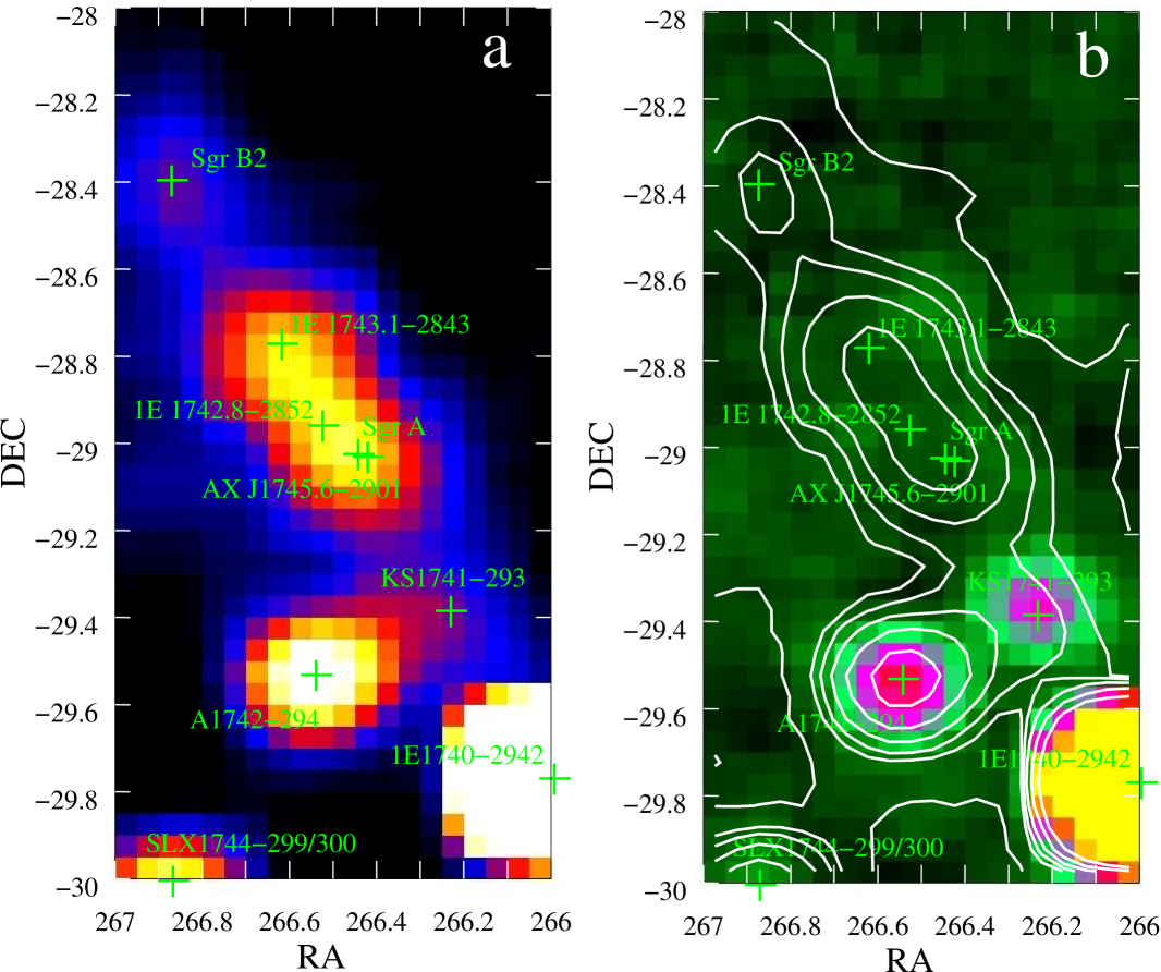
Figure 1: (a). Intensity image of the GC region in 20-60 keV energy band. Black corresponds to zero flux, white to the flux $\geq 1$ cnt/s. Total exposure time is about $2.4$ Ms. (b)20-60 keV variability image of the GC region. Value of each pixel corresponds to the reduced $\chi^{2}$ value for the fit of the detected flux in this pixel by a constant. Black corresponds to the values of $\chi^{2}=1$ while yellow corresponds to $\chi^{2}=4$. Contours show the 20-60 keV flux (in logarithmic scale) from the same region of the sky.

One can see that from all sources visible on the intensity map, Fig. 1a, only 3 appear at the variability map, Fig. 1b. Among the variable sources are the well-known X-ray binaries, 1E 1740.7-2942, A 1742-294 and KS 1741-293. The variability indexes $V=\Delta F/F$ for these sources are $0.07$, $0.22$ and $0.59$, respectively. One can see that in spite of large excess $\chi^{2}_{red}$ at the location of the brightest source, the X-ray binary 1E 1740.7-2942, the source flux varies at the level of only about 7%. This implies an important limitation for the possible applications of the method of variability search described above: the X-ray binaries which produce much lower flux (e.g. at the level of KS 1741-293) but have similar variability properties as 1E 1740.7-2942, would not be localized in the variability map, because the excess of $\chi^{2}_{red}$ produced by such sources would be less than the statistical scatter of the $\chi^{2}_{red}$ values over the image pixels.

In this respect the source 1E 1743.1-2843 is an interesting example. As one can see, this source is not detected in the variability image. Calculating the upper limit on the variable fraction of the source flux, $\Delta F$, along the lines explained above, one gets an upper limit on possible variability at the level of $8$%. 1E 1743.1-2843 was discovered by the Einstein Observatory (Watson et al. (1981)). Its spectral characteristics suggest an interpretation as a neutron star LMXB (Cremonesi et al. (1999)) while its luminosity suggests that the source should belong to the Atoll-class sources and should exhibit Type-I X-ray bursts. The lack of substantial variations of the X-ray flux from this source during the last 20 yr of observations questions such an interpretation (Porquet et al. 2003a ). The lack of variability in 20-60 keV energy band also argues against the neutron-star X-ray binary interpretation for this source, although a definite conclusion would be possible only after a systematic study of variability properties of LMXBs detected by the INTEGRAL.

4 Non-variability of the GC source.

The GC itself (the source IGR J1745.6-2901) also does not appear in the variability map. The upper limit on the variable contribution to the flux can be obtained, as it is explained above, from the typical value of the variance in a single ScW of duration of $\sim 2$ ksec in 20-60 keV band (Bodaghee et al. (2004)), $\Sigma_{b}^{2}\simeq 10^{-10}$ erg/(cm² s). Dividing $\Sigma_{b}^{2}$ by $\sqrt{N}$ and taking into account the systematic “renormalization” by a factor $\simeq 1.4$ which has to be applied to the image Fig. 1b (see the discussion at the end of the previous section), we find an upper limit to the variable contribution at the level of $V=\Delta F/F\leq 0.08$, or, equivalently, $\Delta F\leq 5\times 10^{-12}$ erg/(cm² sec) in the 20 to 60 keV band.

This upper limit is obtained under certain assumption about the variability type (Gaussian fluctuations around the mean flux). At the same time, if the variable emission is of different type, the above upper limit would not apply. For example, if the source has exhibited one or two powerful flares during the whole observation period, the amplitude of the flares can not be deduced from the statistical fluctuations of the signal.

The non-detection of variability of IGR J1745.6-2901 indicates that the main contribution to the hard X-ray flux from this source possibly comes from an extended region around the supermassive BH, rather than from the direct vicinity of the BH horizon. Indeed, simple powerlaw extrapolation of the observed X-ray flux from Sgr A* shows that during the brightest flares the 10-100 keV flux would be roughly at the level detected by the INTEGRAL. However, in this case the hard X-ray flux should vary by $\sim 100$% at the ksec time scale, which is well beyond the upper limit found above. At the same time, the flux in 1-10 keV energy band is dominated by the diffuse emission and a simple powerlaw extrapolation of the diffuse X-ray signal to hard X-ray band is in good agreement with the INTEGRAL data (see below).

As it is discussed in the Introduction, the diffuse X-ray emission from the region around Sgr A* contains a hard component of unclear nature. The 8 keV “temperature” of this hard component is at the upper end of the energy band probed by the X-ray telescopes and in order to prove the thermal nature of this component one has to observe the exponential cut-off in the spectrum above 10 keV. The analysis of INTEGRAL spectrum of IGR J1745.6-2901 shows that such a sharp cut-off is not observed.

The 20-200 keV spectrum of IGR J1745.6-2901 is shown on Fig. 2 together with XMM-Newton spectrum in 3-10 keV energy band extracted from a circular region of radius $R=6^{\prime}$ around the GC (chosen to match the angular resolution of ISGRI imager on board of INTEGRAL).

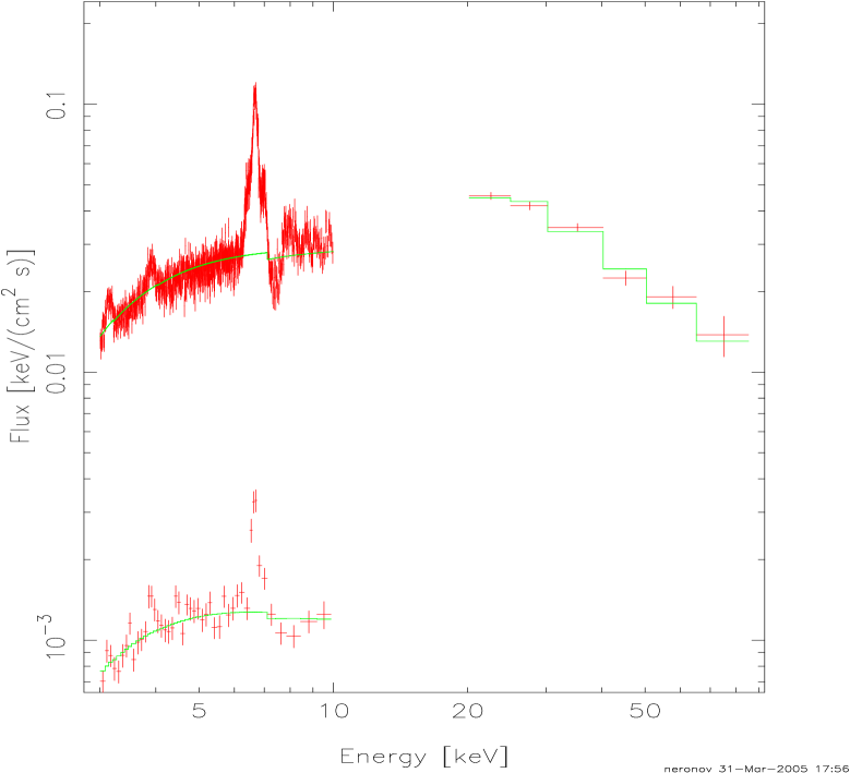
Figure 2: ISGRI spectrum of IGR J1745.6-2901 (the GC) in the 20-200 keV energy band. Also shown is the XMM-Newton spectrum (diffuse emission plus point sources) from the circular region of the radius $6^{\prime}$ (about the size of the point spread function of ISGRI). Strong line in the XMM-Newton data is the 6.4 keV Fe K_α line. For comparison we show also the XMM-Newton spectrum extracted from a circular region of the radius 15” centered on Sgr A* (the lower curve in 3-10 keV band).

The XMM-Newton Observation Data Files (ODFs), obs_id 0111350101, were obtained from the online Science Archive http://xmm.vilspa.esa.es/external/xmm_data_acc/xsa/index.shtml. The data were processed and the event-lists filtered using xmmselect within the Science Analysis Software (sas) v6.0.1. The 20-200 keV spectrum can be fit by a simple power law model with the photon spectral index $\Gamma_{20-200}=3.0\pm 0.1$ and flux $F_{20-200}=(4\pm 2)\times 10^{-11}$ erg/(cm² s). However, a broken power-law provides a better fit to the INTEGRAL data. The broken power law with a break energy at $E_{break}=26\pm 1$ keV is characterized by a low energy spectral index $\Gamma_{low}=1.85^{+0.02}_{-0.06}$, and a high-energy spectral index $\Gamma_{high}=3.3\pm 0.1$. It provides the best simultaneous fit to the XMM-Newton and INTEGRAL data. The intercalibration factor between the two instruments is just $1.2$ which indicates that 20-200 keV flux detected by INTEGRAL matches well the 1-10 keV flux collected from the region of the size about the point spread function of ISGRI.

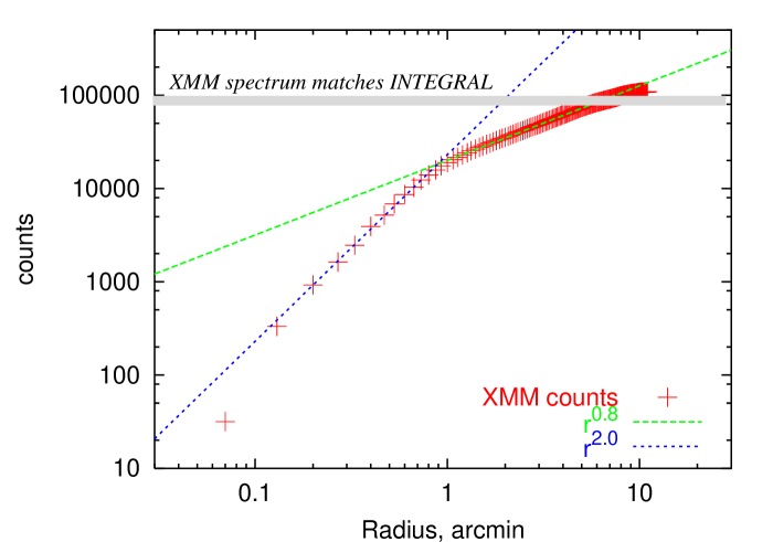
Figure 3: Dependence of the (background corrected) X-ray flux collected from a disk on the radius of the disk centered at Sgr A* in the XMM-Newton image of the Galactic Center. Thin solid line shows the fit $F\sim r^{0.8}$ for the radius range $1^{\prime}<r<10^{\prime}$. Dashed line shows the fit $F\sim r^{2}$ for the radius range $r<1^{\prime}$. Thick gray line shows the flux level at which the XMM-Newton spectrum matches the INTEGRAL spectrum with inter-calibration factor $\simeq 1$.

It is important to note that because of the presence of diffuse emission component around the Galactic Center, the normalization of the XMM-Newton flux depends strongly on the size of the region from which the spectrum is extracted. For example, if one collects the flux from a disk-like region of the radius $r$ centered on the Galactic Center, the flux grows as $r^{2}$ for $r<1^{\prime}$, see Fig. 3. From Fig. 3 one can see that the mismatch between the normalization of the INTEGRAL spectrum and XMM-Newton spectrum collected from the $r\simeq 1^{\prime}$ disk would be a factor of $\simeq 10$. For the disk radii $r>1^{\prime}$ the flux grows proportionally to $r$. The fact that the XMM-Newton spectrum matches the INTEGRAL spectrum when the disk radius reaches $r\simeq 6^{\prime}$ has an important implication for the physics of diffuse hard X-ray emission.

5 The nature of extended non-thermal hard X-ray emission around the GC.

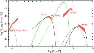
Figure 4: Broad band spectrum of diffuse emission from the Galactic Center region. Radio data are from (Pedlar et al. (1989)), HESS data are from (Aharonian et al. (2004)) and EGRET data are from (Mayer-Hasselwander et al. (1998)). Thin (black) line shows synchrotron and IC emission from electron powerlaw electron distributions with cutoff energy $E_{0}=30$ TeV, in magnetic field $B=3\times 10^{-4}$ G. Thin dashed line is the bremsstrahlung emission from the same population of electrons, assuming typical matter density $n\simeq 10^{4}$ cm^-3. Thick (green) line: the cut-off energy $E_{0}=3$ GeV, magnetic field $B=3\times 10^{-5}$ G. Thick dashed line shows the bremsstrahlung component assuming the density $n\simeq 10^{3}$ cm^-3.

We have seen in the previous sections that several complementary arguments indicate that the hard X-ray emission from the GC detected by INTEGRAL originates from an extended region around the supermassive black hole. The inter-calibration factor of order of $1$ between XMM-Newton and INTEGRAL spectra can be achieved only if the XMM-Newton flux is collected from a circular region of the radius $r\simeq 6^{\prime}$. This means that the size of the hard X-ray extended emission region is about $D\simeq 20$ pc.

In order to understand the mechanism of diffuse nonthermal 10-100 keV emission from the inner $\sim 10$ pc of the Galaxy, it is useful to recall that this region is characterized by quite special astrophysical conditions. It is quite densely populated with giant molecular clouds and the typical gas/dust density throughout the region is $n\sim 10^{4}$ cm^-3 (see (Metzger et al. (1996)) for a review). Most of the estimates of magnetic field are in the range $B\sim 10^{-4}-10^{-3}$ G (Yusef-Zadeh et al. (1996)), much stronger than the typical Galactic magnetic field. Besides, the density of the infrared-optical background in this region, $U_{ir-o}\sim 10^{2}-10^{3}$ cm^-3 (Cox and Laureijs (1988)), is more than two orders of magnitude higher than the density of cosmic microwave background radiation. Such “exotic” conditions should be taken into account in the modeling of physical processes leading to the emission of diffuse non-thermal X-rays.

Among the possible emission mechanisms, synchrotron radiation from electrons of energies $E_{e}\sim 10^{13}-10^{14}$ eV is the most plausible candidate. The typical energy of synchrotron photons produced by such electrons is $E_{syn}\simeq 50(B/10^{-4}$ G$)(E_{e}/10^{14}$ eV$)^{2}$ keV. The synchrotron cooling time of electrons emitting at 10 keV is $t_{syn}\simeq 16(B/10^{-4}$ G$)^{-3/2}(\epsilon/10$ keV$)^{-1/2}$ yr. One can see that the cooling time is too short for electrons accelerated near the supermassive black hole to spread over the emission region of the size $D\sim 20$ pc if one assumes diffusion of electrons injected by a central source. Naively, to overcome this difficulty, one would assume a lower magnetic field strength in the emission region. However, in this case the inverse Compton (IC) flux from electrons which emit synchrotron radiation at $\sim 10$ keV would be stronger than the TeV flux from the GC detected by HESS. Thus, within the synchrotron scenario one has to assume that either magnetic field in the emission region is mostly ordered, so that electrons escape along the magnetic field lines, rather than diffuse in the random magnetic field, or that 10-100 TeV electrons are injected not by a point source at the location of the GC, but throughout the whole extended region of the size $\sim 10-20$ pc. Possible mechanism leading for such “extended injection” is e.g. cascading of the 1-100 TeV gamma quanta on dense infrared photon background in the central 20 pc of the Galaxy (Neronov et al. (2002); Aharonian and Neronov (2005)). Otherwise, electrons can be accelerated in the shell of supernova remnant Sgr A East, whose size is about 5 pc.

Large density of the infrared-optical photon background and of the molecular gas in the emission region lead to significant IC and bremsstrahlung emission from the $10^{13}-10^{14}$ eV electrons. The results of calculation of the broad-band spectrum synchrotron-IC-bremsstrahlung emission from the inner 20 pc of the Galaxy are shown in Fig. 4. One can see that the expected IC and bremsstrahlung fluxes are strong enough to match the observed level of the TeV emission from the GC. If the TeV flux detected by HESS is produced via the above mechanism, it should be not variable, since the IC and bremsstrahlung flux also come from the extended region of the size of several tens of kiloparsecs. The (non)variability of the TeV signal from the GC can be tested with future HESS observations.

Since the synchrotron emission results in efficient cooling of the high-energy electrons, all the power supplied by the supermassive black hole is dissipated with almost 100% efficiency in the form of the hard non-thermal X-ray emission. The required power of the supermassive black hole in the “synchrotron-IC-bremsstrahlung” scenario is just $P_{syn}\simeq 10^{36}$ erg/s, about the total power of Sgr A* observed in infrared. Thus, the above scenario is the most “economic” one.

Other possible mechanisms of non-thermal 10-100 keV emission appear to be much less efficient. For example, if one tries to explain the observed hard X-ray flux with the bremsstrahlung, one finds immediately that for moderately relativistic electrons which can emit bremsstrahlung radiation at $20-50$ keV, the bremsstrahlung cooling rate is some 5 orders of magnitude less than the Coulomb loss rate, which means that the bremsstrahlung is very energetically inefficient mechanism of powering the nonthermal hard X-ray emission. The supermassive black hole should produce the power at the level of $L_{BH}\geq 10^{5}L_{X-ray}\sim 10^{41}$ erg/s in this scenario. Although such a luminosity is still much below the Eddington luminosity of a $4\times 10^{6}M_{\odot}$ black hole, it is orders of magnitude higher than the observed luminosity of Sgr A* in the wide photon energy range from radio to very-high-energy gamma-rays.

The possibility that the observed non-thermal emission is produced via IC scattering of the dense infrared photon background is also unsatisfactory. The IC cooling time for electrons emitting in the 10-100 keV band, $t_{IC}\simeq 3\times 10^{6}\left(U_{ir-o}/(100\mbox{ eV/cm}^{3})\right)^{-1}(E_{e}/1$ GeV$)^{-1}$ yr, is much larger than the bremsstrahlung cooling time, $t_{br}\simeq 4\times 10^{3}(n/10^{4}$ cm${}^{-3})^{-1}$ yr. This means that (1) the supplied power should be 2-3 orders of magnitude higher than the observed hard X-ray luminosity (depending on the assumptions about the dust density) and (2) the hard X-ray IC emission should be accompanied by much stronger 100 MeV bremsstrahlung emission. In fact, the predicted bremsstrahlung flux is at least an order of magnitude higher than the GC flux found in the 100 MeV-GeV band by EGRET (see Fig.4).

Thus, the synchrotron radiation is the most probable mechanism of the diffuse hard X-ray emission from the inner 20 pc of the Galaxy. In order to test the above synchrotron-IC-bremsstrahlung scenario, one has to study the correlation of the spatial distributions of 20-100 keV and 1-10 TeV fluxes. Although it is quite difficult to analyze extended sources with the coded mask instruments, like INTEGRAL, it would be interesting to extract the information on the extension of the source directly from the 10-100 keV data (not from the matching with the lower-energy spectrum, like it is done above). We leave this question for future study.

References

- Aharonian et al. (2004) Aharonian F.; Akhperjanian A. G.; Aye K.-M. et al., 2004, A& A, 425, L13
- Aharonian and Neronov (2005) Aharonian F., Neronov A., 2005, Ap.J. 619, 306
- Baganoff et al. (2001) Baganoff F. K., Bautz M. W., Brandt W. N., et al. 2001, Nature, 413, 45
- Bélanger et al. (2004) Beĺanger G., Goldwurm A., Goldoni P., et al. 2004, Ap.J., 601, L163
- Bodaghee et al. (2004) Bodaghee A., Walter R., Lund N., Rohlfs R., 2004, in “The INTEGRAL Universe”, Proc. 5th INTEGRAL Workshop, ESA SP-552
- Courvoisier et al. (2004) Courvoisier T. J.-L., Walter R., Beckmann V., et al. 2003, A&A 411, L53
- Cox and Laureijs (1988) Cox P., Laureijs R., 1989, IAU-Symp 136, 121
- Cremonesi et al. (1999) Cremonesi D. I., Mereghetti S., Sidoli L., Israel G. L., 1999, A& A, 345, 826
- Genzel et al. (2000) Genzel R., Pichon C., Eckart A., et al. 2000, MNRAS, 317, 348
- Genzel et al. (2003) Genzel R., Schödel R., Ott T., et al. 2003, Nature, 425, 934
- Ghez et al. (2000) Ghez A. M., Morris M., Becklin E. E., et al. 2000, Nature, 407, 349
- Goldwurm et al. (2003) Goldwurm A. et al. 2003, ApJ, 584, 751
- Goldwurm et al. (2004) Goldwurm A., Belanger G., Goldoni P., Paul J., et al. 2004, in Proc. of 5-th INTEGRAL workshop “The INTEGRAL Universe”, Munich, [astro-ph/0407264]
- Mayer-Hasselwander et al. (1998) Mayer-Hasselwander H. A., Bertsch D. L., Dingus B. L., et al. 1998, A& A, 335, 161
- Melia and Falcke (2001) Melia F., Falcke H. 2001, ARA& A, 39, 309
- Metzger et al. (1996) Metzger P.G., Duschl W.J., Zylka R. 1996, ARA& A, 7, 289
- Muno et al. (2004) Muno M.P., Baganoff F. K., Bautz M. W., et al., 2004, ApJ. 613, 326.
- Narayan et al. (2002) Narayan R., Quataert E., Igumenshchev I. V.; Abramowicz M. A., 2002, ApJ, 577, 295
- Neronov et al. (2002) Neronov A., D. Semikoz D., Aharonian F., Kalashev O., 2002, Phys. Rev. Lett., 89, 051101
- Pedlar et al. (1989) Pedlar A., Anantharamaiah K.R., Ekers R.D., Goss W.M., et al., 1989, ApJ, 342, 769
- Porquet et al. (2003) Porquet D., Predehl P., Aschenbach B., et al. 2003, A& A, 407, L17
- (22) Porquet D., Rodriguez J., Corbel S. et al. 2003, A& A, 406, 299
- Schödel et al. (2002) Schödel R., Ott T., Genzel R., et al. 2002, Nature, 419, 694
- Watson et al. (1981) Watson M. G., Willingale R., Hertz P., Grindlay J. E., 1981, ApJ 250, 142
- Yusef-Zadeh et al. (1996) Yusef-Zadeh F., Roberts D.A., Goss W.M., Frail D.A., Green A.J. 1996, ApJ, 466, L25
- Zylka et al. (1995) Zylka R., Mezger P. G., Ward-Thompson D., et al. 1995, A& A, 297, 83