Imaging Bright Spots in the Accretion Flow Near the Black Hole Horizon of Sgr A*

Abstract

Images from the vicinity of the black hole horizon at the Galactic centre (Sgr A*) could be obtained in the near future with a Very Large Baseline Array of sub-millimetre telescopes. The recently observed short-term infrared and X-ray variability of the emission from Sgr A* implies that the accretion flow near the black hole is clumpy or unsteady. We calculate the appearance of a compact emission region (bright spot) in a circular orbit around a spinning black hole as a function of orbital radius and orientation. We find that the mass and spin of the black hole can be extracted from their generic signatures on the spot image as well as on the lightcurves of its observed flux and polarisation. The strong-field distortion remains noticeable even when the spot image is smoothed over the expected $\sim 20\,\mu{\rm as}$ resolution of future sub-millimetre observations.

1 Introduction

Despite its successes, there has not yet been a satisfactory test of general relativity in the strong gravity limit. By their very nature, studies of black holes are likely to provide the best opportunity for constraining strong field relativity. Unfortunately, current attempts to do this rely upon modelling the accretion flow and are thus indirect (see, e.g., Narayan & Heyl, 2002; Tanaka et al., 1995; Reynolds & Nowak, 2003; Pariev et al., 2001).

Of these, the most direct method involves observations of line-like features in the X-ray spectra of black hole candidates, typically interpreted as the Fe K$\alpha$ fluorescence line, broadened as a result of the Keplerian motion of the disk and frame dragging due to the rotation of the black hole (see, e.g., Reynolds & Nowak, 2003; Pariev et al., 2001). The lack of a correlation between the variability in the soft X-ray continuum and the line emission implies that the simplest model used for the interpretation of the observations is incomplete (see, e.g., Weaver et al., 2001; Wang et al., 2001, 1999; Chiang et al., 2000; Lee et al., 2000), though attempts to rectify this situation with the inclusion of gravitational lensing have been made (Matt et al., 1997). The case is further complicated by the existence of alternative interpretations (see, e.g., Elvis, 2000; You et al., 2003).

General relativistic effects can also play a substantial role in the polarisation properties of Thomson thick disks (see, e.g. Connors et al., 1980; Laor et al., 1990; Bao et al., 1997). Therefore, detailed spectropolarimetric observations may shed light on both the physics of the accretion flow and the curvature of space-time. However, these necessarily require an accretion model and consequently suffer from considerable uncertainties associated with the accretion physics.

In contrast, it may be possible to directly image a black hole, and thus measure the space-time curvature down to the photon orbit, the radius at which photons execute a circular orbit, $3GM/c^{2}$ for a Schwarzschild black hole and down to $GM/c^{2}$ for a maximally rotating Kerr black hole (Falcke et al., 2000). The black hole in the Galactic centre provides the best candidate for such an observation as it possesses the largest apparent size on the sky, with $GM/c^{2}$ corresponding to an angular scale of $\sim 5\,\mu{\rm as}$. Within the next decade it is expected that a Very Large Baseline Array (VLBA) at sub-millimetre wavelengths (where scattering is no longer the limiting factor) will exist which is expected to provide $\sim 20\,\mu{\rm as}$ resolution (Greenhill, 2005; Miyoshi et al., 2004).

Earlier theoretical work has focused on optically thin, azimuthally symmetric accretion flows, which are generically expected to show a shadow around the black hole (e.g., Falcke et al., 2000; Takahashi, 2005, 2004; Beckwith & Done, 2005). However, numerical general-relativistic magnetohydrodynamic simulations of accretion flows suggest that the region near the innermost stable circular orbit (ISCO) may be strongly inhomogeneous (see, e.g., De Villiers et al., 2003). Indeed, recent observations of Sgr A* in the infrared and X-ray bands revealed flaring activity on short time scales (Ghez et al., 2004; Eckart et al., 2004; Genzel et al., 2003; Porquet et al., 2003; Aschenbach et al., 2004; Goldwurm et al., 2003; Baganoff et al., 2001) indicating strong inhomogeneities in the emission close to the black hole horizon. Computations of the light curves of inhomogeneous accretion flows have been performed in the context of quasars and X-ray binaries more generally (Bao et al., 1998, 1997), but without providing images to be compared with future observations and without studying the dependence of the light curve on the black hole parameters.

In this paper, the unpolarised and polarised light curves and images are computed for an optically thick emitting sphere at a number of radii, viewing angles, and black hole spins. While this may strictly apply for a star orbiting a supermassive black hole, it should be understood that our treatment is a proxy for any mechanism which enhances the emission in a compact region of space (e.g., due to reconnection events, over densities in mass or magnetic field strength).

The method by which rays are traced, the radiative transfer performed, and the optically thick sphere is modelled are discussed in section 2. Section 3 compares the expected light curves (both polarised and unpolarised) for a number of orbits, viewing angles, and black holes spins. Images and centroid motions are presented in sections 4 and 5, respectively. Finally, concluding remarks are summarised in section 6.

In what follows, the metric signature is taken to be $(-+++)$, and geometrised unites are used ($G=c=1$).

2 Computational Methods

Due to the complexities introduced by the Kerr metric, in the strong field limit, images of the accretion flow are most readily obtained via numerical methods. This computation may be succinctly segregated into the problems of tracing null geodesics, performing the radiative transfer along these rays, and modelling the inhomogeneity (in this case an optically thick sphere). The first two of these are treated in subsection 2.1, and the third in subsection 2.2.

2.1 Ray Tracing & Radiative Transfer

The light rays are traced in curved space following the scheme of Broderick & Blandford (2003) (for which tracing null geodesics is a limiting case), as well as the radiative transfer method of Broderick & Blandford (2004). Below, only the essential aspects are summarised.

Null geodesics are constructed by integrating the equations

$$\frac{dx^{\mu}}{d\lambda} =f(r)k^{\mu}$$

$$\frac{dk_{\mu}}{d\lambda} =-f(r)\left(\frac{1}{2}\frac{\partial k^{\nu}k_{\nu}}{\partial x^{\mu}}\right)_{k_{\alpha}}\,,$$ (1)

where the partial differentiation is taken holding the covariant components of the wave four-vector, $k_{\mu}$, constant, and

$$f(r)=r^{2}\sqrt{1-\frac{r_{h}}{r}}\,,$$ (2)

(where $r_{h}$ is the horizon radius) simply reparameterises the affine parameter, $\lambda$, along the ray to avoid singular behaviour near the horizon. An explicit demonstration that $x^{\mu}(\lambda)$ reproduce the null geodesics can be found in Broderick & Blandford (2003).

Typically, polarised radiative transfer is performed using the Stokes parameters. However, since these are not Lorentz scalars, in relativistic environments they are not ideal. In contrast, the photon distribution function ($\propto I_{\nu}/\nu^{3}$) is a Lorentz scalar, and thus much simpler to evolve along the null geodesics. As shown in Broderick & Blandford (2004), it is possible to define analogues of the photon distribution function for the rest of the Stokes parameters using an orthonormal tetrad propagated along the null geodesics.

While the numerical scheme utilised here is not optimized for this particular problem, it has the virtue of already being implemented and tested in the context of imaging accreting black holes.

2.2 Optically Thick Sphere

An inhomogeneity in the accretion flow is modelled as an optically thick sphere orbiting around the central black hole. The surface of the inhomogeneity is given implicitly by

$$\Delta r^{\mu}\Delta r_{\mu}+\left(u_{S}^{\mu}\Delta r_{\mu}\right)^{2}=R_{S}^{2}$$ (3)

where $\Delta r^{\mu}\equiv r^{\mu}-r_{S}^{\mu}$ is the displacement from the sphere centre, located at $r_{S}^{\mu}$, moving with velocity $u_{S}^{\mu}$, and $R_{S}$ is the radius of the sphere. The second term accounts for the length contraction. In the limit that $\Delta r^{\mu}\Delta r_{\mu}\ll r$ this definition indeed produces a sphere in the comoving frame. For $\Delta r^{\mu}\Delta r_{\mu}\sim r$ the surface defined by equation (3) necessarily departs from sphericity (since the $\Delta r^{\mu}\Delta r_{\mu}$ is only the differential line element), and thus in reality is only quasi-spherical. However, considering the level of approximation inherent in treating the inhomogeneity as a sphere in the first place, the added simplicity outweighs a more detailed effort to produce a true sphere. Here a value of $R_{S}=1.5M$ is used, which is sufficiently compact to reveal the strong field effects of interest in this study.

Since the sphere is an extended body, it cannot have a uniform velocity if it is to remain coherent. Here all points upon the surface of the sphere are taken to have the same angular velocity as measured by the Boyer-Lindquist observer, i.e., the same $u_{S}^{\phi}/u_{S}^{t}$, ensuring that all parts of the sphere execute an orbit in the same amount of observer time. An explicit proof that this ensures that the sphere does not shear can be found in Broderick & Blandford (2004). The velocity of the centre of the sphere was taken to be that associated with the stable circular orbit at $r_{S}^{\mu}$.

Images are produced by tracing a bundle of parallel rays back from a screen far from the black hole. Rays that impinged upon the sphere were given an intensity (subsequently transformed into a photon distribution function) governed by the Rayleigh-Jeans law,

$$I_{\nu}=2\frac{\nu^{2}}{c^{2}}kT\,,$$ (4)

where $\nu=-u_{\mu}k^{\mu}/2\pi$ and the temperature was assumed to be proportional to its virial value:

$$T\propto-\left(u_{t}-\frac{1}{\sqrt{-g^{tt}}}\right)\,,$$ (5)

where $g^{\mu\nu}$ are the contravariant components of the metric.

Polarisation measurements place an additional observational constraint upon the emission and propagation physics. Because the polarisation is parallel–propagated along the ray, it is especially sensitive to the effects of strong gravity. However, any discussion of polarisation must be prefaced with the caveat that there will be considerable uncertainty in the emitted polarisation, e.g., due to the emission process (synchrotron or Compton scattering), and the geometry of the emitting region (tangled magnetic fields, thick accretion disks, etc). Because of this large uncertainty, a simple fiducial polarisation model is adopted. For the purpose of investigating the generic effects of strong lensing upon the polarisation, the emitted polarisation fraction is set to be constant and polarised orthogonally to the spin axis of the hole (also the orbital axis). Such a geometry might be expected, e.g., when the primary emission mechanism is synchrotron, and the magnetic field is vertically aligned. The polarisation may be substantially reduced in the presence of realistic field geometries, alternate polarising mechanisms, or radiative transfer effects such as Faraday rotation or depolarisation. Nonetheless, this provides some insight into the possible complexity that may arise in the polarised spectrum.

3 Light Curves

Although this paper is primarily concerned with resolved images, considerable information can be extracted from the unresolved unpolarised and polarised light curves. Since obtaining light curves doees not require imaging capabilities, and thus is likely to be technically easier, they are discussed first.

3.1 Unpolarised Flux

In general, the shape of the light curve in its entirety is required to make statements regarding the parameters of the black hole and the orbit. Nevertheless, some of these parameters leave their strongest signatures on particular portions of the light curves.

Any gravitational lensing transient is characterised by a time scale and a magnification. For a compact bright spot on a circular orbit about a black hole, the former is set by the period of the orbit,

$$P=2\pi\left(r_{S}^{3/2}+a\right)\,,$$ (6)

where $r_{S}$ is the orbital radius of the spot and a positive Kerr spin parameter, $a$, corresponds to prograde orbits. For a given $a$, it is straightforward to determine the radius of the orbit. This is readily apparent in Figure 1 in which the magnification (i.e., the integrated flux normalised by its time-averaged value) is plotted as a function of time for orbital radii of $6M$, $8M$, and $10M$ around a Schwarzschild black hole.

Figure 1: The magnification (bottom), polarisation fraction (middle), and polarisation angle (top) as functions of time for orbital radii of $6M$ (solid), $8M$ (long dash), and $10M$ (short dash) around a Schwarzschild black hole viewed from $45^{\circ}$ above the orbital plane. A polarisation angle of $180^{\circ}$ is orthogonal to the orbital plane (see Figure 7). The time axis is set so that a single orbital period of the $10M$ case is shown. For a black hole mass of $4\times 10^{6}{\rm M}_{\odot}$ (as in Sgr A*), the time unit is $M=20\,{\rm s}$.

While the magnification does vary with orbital radius, it is a stronger indicator of the inclination of the orbit relative to the line of sight (not to be confused with orbits lying out of the equatorial plane of a Kerr black hole). This is shown in Figure 2 in which the magnification is shown for viewing angles ranging from edge on ($0^{\circ}$) to nearly face on ($89^{\circ}$). In addition to the strong magnification for orbits which pass directly behind the black hole, there is a second feature near $t\simeq-30M$ resulting from those null geodesics which make a complete orbit before escaping to infinity. The significance of these in the context of the Fe K$\alpha$ lines has been previously noted by Beckwith & Done (2005). Here it provides a second signature of the strong bending of light, though only for orbits that are viewed nearly edge on.

Figure 2: The magnification (bottom), polarisation fraction (middle), and polarisation angle (top) as a function of time for an orbit at $6M$ around a Schwarzschild black hole viewed from $0^{\circ}$ (solid), $22.5^{\circ}$ (long dash-dot), $45^{\circ}$ (dash-dot), $67.5^{\circ}$ (long dash), $80^{\circ}$ (short dash) and $89^{\circ}$ (dotted) above the orbital plane. The time axis is set so that a single orbital period is shown.

The dependence of the magnification light curve upon $a$ is presented in Figures 3 and 4. In Figure 3, different spin parameters ($a=0$, $0.5$, $0.998$) are compared at a fixed radius in Boyer-Lindquist coordinates, namely $6M$. In this case, higher black hole spins tend to demagnify the source slightly. However, this may be of secondary significance when compared to the fact that for higher $a$, stable circular orbits extend closer to the horizon. Indeed, as seen in Figure 4, placing the orbits at the ISCO results in a net increase in the maximum magnification (and a substantially reduced orbital period!).

Figure 3: The magnification (bottom), polarisation fraction (middle), and polarisation angle (top) as a function of time for an orbit at $6M$ around a Kerr black hole with $a=0$ (solid), $0.5$ (long dash), and $0.998$ (short dash) viewed from $45^{\circ}$ above the orbital plane. The time axis is set so that a single orbital period of the $a=0.998$ case is shown.

Figure 4: The magnification (bottom), polarisation fraction (middle), and polarisation angle (top) as a function of time for orbits at the prograde ISCO of the Kerr space-time $a=0$ (solid), $0.5$ (long dash), and $0.9$ (short dash) viewed from $45^{\circ}$ above the orbital plane. The time axis is set so that a single orbital period of the $a=0$ case is shown.

For rapidly rotating black holes one would expect a difference in the lensing signature of prograde and retrograde orbits. This will be mitigated somewhat by the fact that the retrograde ISCO moves out considerably, reaching $\sim 9M$ for the maximally rotating case. Nonetheless, as seen in Figure 5, there are quantitative differences in the magnification similar to those seen when the spin is varied (cf. Figure 3) as expected.

Figure 5: The magnification (bottom), polarisation fraction (middle), and polarisation angle (top) as a function of time for prograde (solid line) and retrograde (long-dash line) orbits at the retrograde ISCO of the Kerr space-time for $a=0.5$ (thick line) and $a=0.998$ (thin line) viewed from $45^{\circ}$ above the orbital plane. The time axis is set so that a single orbital period of the prograde $a=0.998$ case is shown. In all cases the direction of the orbital motion is the same (i.e., the retrograde orbits are generated by reversing the spin of the hole).

3.2 Polarised Flux

In addition to the magnification, Figures 1–4 also show the fractional change in the emitted polarisation and the polarisation angle for the fiducial polarisation model described in section 2.2 (and subject to the caveats presented at the end of that section). In general, the polarisation fraction and polarisation-angle light curves show considerable structure. The variability results primarily from special relativistic aberration associated with the rapid orbital motion, coupled with the choice of the emitted polarisation. This effect is substantially amplified by both gravitational lensing (which allows many viewing angles to be sampled) and general relativistic transfer effects (which rotate the polarisation direction according to the rules of parallel propagation).

The two primary features in the polarisation light curves are the decrease in polarisation fraction (referred to in what follows as the primary minimum) and rotation of the polarisation angle immediately preceding the maximum magnification. Both phenomena result from the development of an Einstein ring/arc, and are thus expected to be generic features. For the configuration considered here, these are a strong function of radius (see, e.g., Figure 1) and viewing angle (Figure 2). The dependence upon viewing angle reaches a maximum when a substantial portion of the rays are incident along the orbital axis (note that due to gravitational lensing this does not occur when the orbit is face on).

A third notable feature is the location of a second minimum due to the development of a secondary ring/arc resulting from rays which complete an orbit before escaping to infinity. This second minimum is considerably shallower than (and lags substantially behind) the primary minimum and should not be confused with the substructure within the primary minimum. The decrease in the polarisation fraction results for reasons similar to those that produce the primary minimum, and is similarly expected to be a generic feature. It is present in Figures 1 and 2, where it leads the primary minimum by $\sim 50M$. However, of greater interest is the strong dependence of this feature upon the structure of the space-time near the photon orbit, and thus its sensitivity to strong-field general-relativity. This is explicitly demonstrated in Figures 3 and 5, in which the lag between the primary and secondary minima is a strong function of black hole spin.

As the orbit becomes more relativistic, a permanent partial ring develops, qualitatively changing the polarisation features. This can be seen in Figure 4. However, it can be more clearly seen in the images, [e.g., Figure 6, panel (e)], and thus is discussed in the following section.

4 Images

In addition to measuring the light curves, future sub-millimetre observations promise to image the inner regions of the Galactic centre at $20\,\mu{\rm as}$ resolution (Greenhill, 2005; Miyoshi et al., 2004). Illustrative images of the orbits are presented in this section. These may be compared with calculations which assume a uniform and steady accretion flow (e.g., Falcke et al., 2000; Takahashi, 2004, 2005).

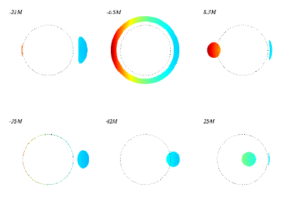
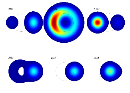
(a)	(b)
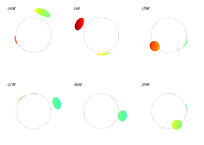
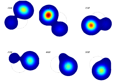
(c)	(d)
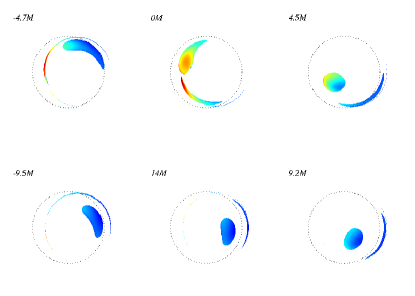
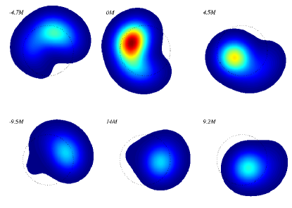
(e)	(f)

Figure 6: Illustrative sequences of intensity maps. Cases (a) & (b) refer to $r_{S}=6M$, $a=0$, viewed in the orbital plane, (c) & (d) refer to $r_{S}=6M$, $a=0$, viewed from $45^{\circ}$ above the orbital plane, and (e) & (f) refer to an orbit at the prograde ISCO for $a=0.9$, also view from $45^{\circ}$ above the orbital plane. Panels on the left are shown at the computed resolution, while panels on the right are smoothed by an instrument resolution of $20\,\mu{\rm as}$ (achievable with a future sub-mm VLBA). For reference, the time as shown in the light curves is listed in the upper-left corner of each map, and the photon capture impact parameter ($\sqrt{27}M$) is shown by the dotted circle.

Figure 6 shows a sequence of six images distributed roughly evenly throughout an orbit for three of the cases discussed in the previous section. In particular the upper panels show an orbit around a Schwarzschild black hole at $r_{S}=6M$ viewed edge on, the middle panels show the same orbit viewed from $45^{\circ}$ above the orbital plane, and the bottom panels show the prograde ISCO of a Kerr black hole with $a=0.9$ viewed from $45^{\circ}$ above the orbital plane. Panels on the left show the computed resolution, while panels on the right are smoothed by a Gaussian filter with full width $4M$ (corresponding to $20\mu{\rm as}$ for Sgr A*) and thus are comparable to those that may be observed within the next decade. Each sequence of images is separately normalised.

While all three cases appear qualitatively different, they share three generic features: brightening due to relativistic beaming, a primary Einstein ring/arc, and a secondary Einstein ring/arc due to photons which complete at least one orbit around the black hole (also complete only on the top panel). The first two features are responsible for the magnification and primary minimum in the unpolarised and polarised light curves, respectively. The third is largely responsible for the secondary minimum in the polarisation fraction. Since the secondary ring/arc is formed by photons which pass near the photon orbit ($3M$ for Schwarzschild, $M$ for maximally rotating Kerr; but see the footnote in section 1), it provides a sensitive test of strong field relativity. As a direct result, the position of the secondary minimum is a diagnostic of the black hole spin, as found in section 3.

Despite the commonalities, there are considerable differences between the three cases shown. The most obvious is that the primary and secondary Einstein rings are incomplete for orbits viewed significantly out of the orbital plane. This results in reduced magnification and polarisation deviations in the lightcurves. In the high spin case, a permanent incomplete ring develops resulting in a qualitative change in the polarised light curves.

As seen in the right-hand panels, these features remain in the smoothed images. Therefore, imaging may be a diagnostic of the orbital and black hole parameters.

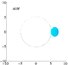
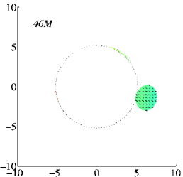
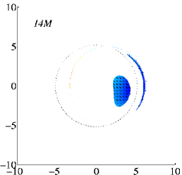
(a)	(b)	(c)
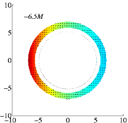
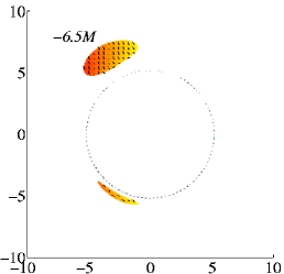
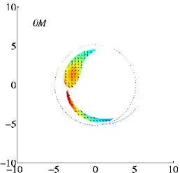
(d)	(e)	(f)

Figure 7: Illustrative polarisation maps for the cases shown in Figure 6. Cases (a) & (d) refer to $r_{S}=6M$, $a=0$, viewed in the orbital plane, (b) & (e) refer to $r_{S}=6M$, $a=0$, viewed from $45^{\circ}$ above the orbital plane, and (c) & (f) refer to an orbit at the prograde ISCO for $a=0.9$, also viewed from $45^{\circ}$ above the orbital plane. The top panels show the polarisation when the emitting sphere is $180^{\circ}$ out of phase with the maximum magnification and thus are indicative of the unlensed polarisation. The bottom plots are illustrative of the polarisation structures within the primary minima in polarisation angle. For reference, the photon capture impact parameter ($\sqrt{27}M$) is shown by the dotted circle. Axes are labelled in units of $M$. For a mass of $4\times 10^{6}{\rm M}_{\odot}$ and distance $8\,{\rm k}{\rm pc}$, appropriate for Sgr A*, the scale $M$ corresponds to $5\,\mu{\rm as}$.

The use of the polarisation as a diagnostic of the space-time structure is illustrated in Figure 7, in which images of the polarisation angles are overlayed upon the intensity maps. For the purpose of comparison, these are shown when the emitting sphere is $180^{\circ}$ out of phase with the maximum magnification (and thus typical of the unlensed polarisation, top) and for a typical point within the primary polarisation minimum (bottom). As seen in the bottom panels, the development of a primary Einstein ring/arc generically rotates the polarisation angle and reduces the integrated polarisation flux. The development of a secondary ring/arc yields similar results, and hence polarisation is sensitive to those image features which probe strong gravity most effectively. Therefore, polarisation can be use to probe the spacetime at the photon orbit, as long as its emission and transfer are understood.

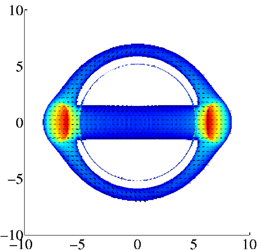
Figure 8: The time average of the intensity and polarisation maps for an edge-on orbit of an emitting sphere at $6M$ around a Schwarzschild black hole. For reference, the photon capture impact parameter ($\sqrt{27}M$) is shown by the dotted circle. Axes are labelled in units of $M$.

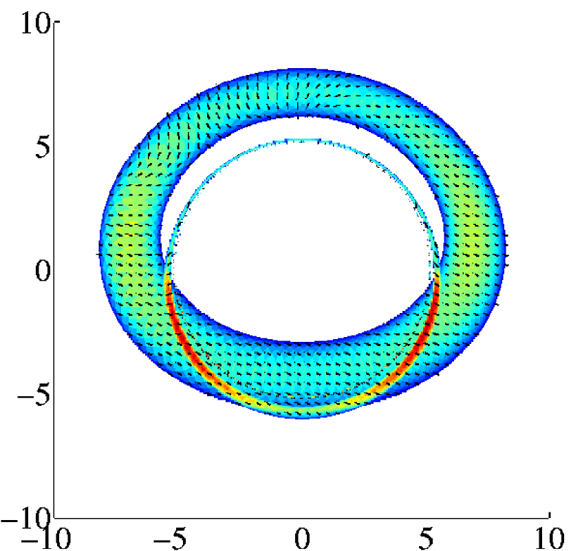
Figure 9: The average of the intensity and polarisation maps for an orbit at $6M$ around a Schwarzschild black hole viewed from $45^{\circ}$ above the orbital plane. For reference, the photon capture impact parameter ($\sqrt{27}M$) is shown by the dotted circle. Axes are labelled in units of $M$.

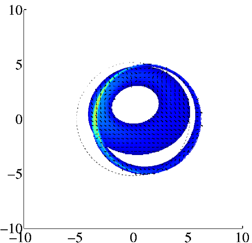
Figure 10: Average of the intensity and polarisation maps for an orbit at the prograde ISCO around a Kerr black hole with $a=0.9$, viewed from $45^{\circ}$ above the orbital plane. For reference, the photon capture impact parameter ($\sqrt{27}M$) is shown by the dotted circle. Axes are labelled in units of $M$.

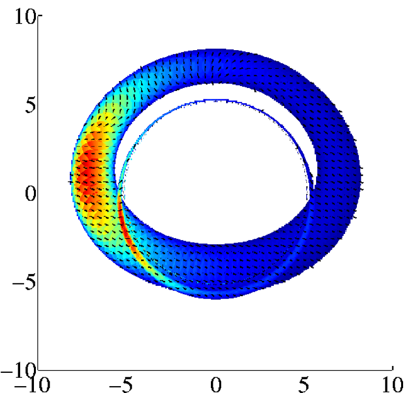
Figure 11: Same as Figure 9, with $I_{\nu}\propto\nu^{-1.3}$. For reference, the photon capture impact parameter ($\sqrt{27}M$) is shown by the dotted circle. Axes are labelled in units of $M$.

The images in Figures 6 and 7 are instantaneous snapshots, and are only observable through exposures that are considerably shorter than the orbital period. Typically, observations will average these images over the instrument integration time. To reflect more realistic circumstances, Figures 8-10 show the intensity and polarisation maps averaged over a full orbit (for the same orbits shown in Figures 6 and 7). These are produced by summing the images used to compute the light curves in section 3. All of these have similar structures: a ring/arc associated with the direct image of the sphere, and a second ring/arc associated with the secondary Einstein ring/arc (which closely follows the photon capture impact parameter).

The remarkable symmetry is an artifact of the emission scheme used; for thermal emission in the Rayleigh-Jeans limit, the special relativistic red-shift is precisely offset by the apparent motion on the sky. This can be explicitly demonstrated for a Schwarzschild black hole by considering a pair of spots moving at a given angle $\theta$ relative to the line of sight with velocities $\beta$ and $-\beta$ and time averaged intensities $\langle I^{+}_{\nu}\rangle$ and $\langle I^{-}_{\nu}\rangle$, respectively. For an emitted spectrum with spectral slope $\alpha$ (i.e., $I_{\nu}\propto\nu^{-\alpha}$) the time averaged intensities are related by

$$\frac{\langle I^{+}_{\nu}\rangle}{\langle I^{-}_{\nu}\rangle}=\frac{I^{+}_{\nu}}{I^{-}_{\nu}}\frac{v_{a}^{-}}{v_{a}^{+}}=\left(\frac{1+\beta\cos\theta}{1-\beta\cos\theta}\right)^{\alpha+2}\,,$$ (7)

where $v_{a}^{\pm}=\beta\sin\theta/(1\mp\beta\cos\theta)$ is the apparent velocity on the sky. Thus, in the Rayleigh-Jeans approximation, $\langle I^{+}_{\nu}\rangle=\langle I^{-}_{\nu}\rangle$ and the images are indeed expected to be symmetric. However, for $\alpha>-2$, as is the case for optically thin synchrotron emission, equation (7) implies a substantial brightness asymmetry. This can be seen explicitly in Figure 11, which is identical to Figure 9 except that $\alpha$ was taken to be $1.3$ (as suggested by infrared and X-ray flare observations, Eckart et al., 2004). However, despite the considerable asymmetry, the morphology of the image remains unchanged. Therefore, measuring the brightness asymmetry provides a method to probe the spectrum of the bright spot. Note that in both cases the symmetry is clearly broken in the polarisation map, and thus polarisation data may be used to infer the direction of the source motion.

The images do not show a clear black hole shadow. This is not a result of approximating an inhomogeneity by an optically thick sphere, but rather due to emission geometry. In particular, the black hole is not everywhere back lit, and hence at positions on the sky where the primary emitting region lies in front of the black hole no shadow is present. Thus, even when the emission is optically thin, it is expected that the image of inhomogeneous accretion flows will qualitatively differ from that produced by a quasi-spherical accretion flow.

It is significant that the average images of the $a=0$ and $a=0.9$ case differ substantially (cf. Figures 9 and 10). In particular, the relative positions of the orbital and secondary ring are shifted. Therefore, the spin of the black hole leads to a relative change in position, which is considerably simpler to measure through sub-millimetre interferometry.

5 Centroids

It should be possible to measure the image centroid with greater precision than the resolution of an image. As seen in Figure 6, the motion of the centroid contains a considerable amount of the information in the image, and thus the path of the centroid provides a diagnostic of the orbital and black hole parameters.

Figure 12: Motion of the centroid of the intensity for circular orbits around a Schwarzschild black hole viewed from $45^{\circ}$ above the orbital plane with radii of $6M$ (solid), $8M$ (long dash), and $10M$ (short dash). For reference, a circle inclined at $45^{\circ}$ is also shown by the dotted lines. Axes are labelled in units of $M$.

Figure 13: Motion of the centroid of the intensity for circular orbits around a Schwarzschild black hole with radius $6M$ viewed from $0^{\circ}$ (solid), $22.5^{\circ}$ (long dash-dot), $45^{\circ}$ (short dash-dot), $67.5^{\circ}$ (long dash), and $89^{\circ}$ (short dash) above the orbital plane. For reference, circles inclined at the various angles are also shown by the dotted lines. Axes are labelled in units of $M$.

Figures 12-15 compare the nearly elliptical centroid paths for various orbital and black hole parameters. The major-axis of the elliptical path is indicative of the orbital radius in a similar way as it is for Newtonian orbits (Figure 12). In general, gravitational lensing will increase the minor-axis. Nevertheless, the minor-axis may be used to infer the orbital inclination (Figure 13). In contrast with variations of the orbital radii, gravitational lensing results in changes that are substantially different from the Newtonian case. Nonetheless, these results suggest that it is indeed possible to place significant constraints upon the orbital parameters from the centroid motion alone.

Figure 14: Motion of the centroid of the intensity for circular orbits in the equatorial plane around a Kerr black hole with radius $6M$ viewed from $45^{\circ}$ orbital plane for Kerr spin-parameters $0$, $0.5$, and $0.998$. For reference, a circle inclined at $45^{\circ}$ is also shown by the dotted line. Axes are labelled in units of $M$.

Figure 15: Motion of the centroid of the intensity for the prograde ISCOs around a Kerr black hole viewed from $45^{\circ}$ above the orbital plane with Kerr spin-parameters $0$ (solid), $0.5$ (long dash), and $0.9$ (short dash). For reference, circles inclined at $45^{\circ}$ at the appropriate radii are also shown by the dotted lines. Axes are labelled in units of $M$.

Of more interest is the possibility of measuring the black hole spin. Given the orbital radius and its period, equation (6) may be used to deduce the black hole spin. Figures 14 and 15 show that this may be constrained by the centroid paths as well. However, except for a feature present only near the maximally rotating case, the paths are very similar, and thus it is likely that imaging will be required to distinguish the different cases. Nevertheless, it is not clear that this is the appropriate comparison because the prograde ISCO moves substantially inwards with increasing black hole spin. Therefore, it may be more suitable to compare different black hole spins at their respective prograde ISCOs, as shown in Figure 15. In this case, there is a morphological change in the centroid paths, in addition to the difference that results trivially from the decrease in orbital radius. As a result, when combined with period measurements, an accurate determination of the centroid path provides a method with which to measure $a$.

Figure 16: Motion of the centroid of the intensity for circular orbits around a Schwarzschild black hole with radius $6M$ viewed from $45^{\circ}$ above the orbital plane for emission models with spectral index $1.3$ (solid), as in Figure 11, and $-2$ (dashed), as in the Rayleigh-Jeans approximation. For reference, a circle inclined at $45^{\circ}$ is also shown by the dotted lines. Axes are labelled in units of $M$.

As suggested by Figure 11, for emission models with spectral index $>-2$ the centroid position will be dominated by the portion of the orbit in which the bright spot is moving towards the observer. This is shown in Figure 16, in which the centroid paths of the Rayliegh-Jeans and $\alpha=1.3$ emission models are compared. Thus, estimates of the orbital parameters from the motion of the centroid may require additional information about the spectrum of the emission. However, as mentioned before, even in the absence of spectroscopy, the spectral index may be obtained from brightness asymmetry in the the time-averaged images (see, e.g., equation 7).

6 Conclusions

The orbit-integrated image of a bright sphere (hot spot) in motion near the horizon of Sgr A* is qualitatively different from the image produced by a quasi-spherical accretion flow. In particular, the time-averaged image of a compact hot spot does not reveal a clear black hole shadow, as found for spherical accretion flows (Falcke et al., 2000).

The evidence for short-term flaring activity in the Galactic centre (Ghez et al., 2004; Eckart et al., 2004; Genzel et al., 2003; Porquet et al., 2003; Aschenbach et al., 2004; Goldwurm et al., 2003; Baganoff et al., 2001), implies that the accretion flow around the horizon of Sgr A* is clumpy or unsteady. In the likely event that the accretion flow has bright spots, imaging of these spots could be utilised as a method for inferring the black hole parameters. In particular, the signature of the secondary Einstein ring/arc in the light curves and the images could potentially be more sensitive to strong gravity effects than imaging the black hole shadow alone. In the time averaged images, black hole spin produces relative offsets between features (see, Figure 10), which are amenable to interferometric imaging in a way that measurements of the shadow are not.

Imaging a bright spot may also independently constrain the mass and distance of Sgr A*. Timing data combined with the projection of the orbit on the sky (or the apparent velocity) allows the measurement of the ratio of Sgr A*’s mass and distance. If the line-of-sight velocity of the inhomogeneity can be determined as well (e.g., from spectral measurements combined with the magnitude of the brightness asymmetry), this degeneracy can be broken.

If the emission is polarised (and the nature of the intrinsic polarisation is understood), light curves and images of the polarisation are strongly dependent upon those features in the image that are produced near the photon orbit. Hence, polarisation in general may be diagnostic of the black hole parameters.

Lastly, even if high precision images are unavailable, measurements of the centroid path coupled with observations of the light curve provide an alternative method by which to determine the black hole spin.

In reality, images of the Galactic centre may be expected to result from inhomogeneities during flaring events superimposed upon a homogeneous background. Thus, the results of this paper are complimentary to previous work. It is therefore likely that observations of both, a black hole shadow between flaring events and the dynamical and/or averaged properties of the images during flaring events, can be coupled to reduce the uncertainty inherent to each.

References

- Aschenbach et al. (2004) Aschenbach B., Grosso N., Porquet D., Predehl P., 2004, A&A, 417, 71
- Baganoff et al. (2001) Baganoff F. K., Bautz M. W., Brandt W. N., Chartas G., Feigelson E. D., Garmire G. P., Maeda Y., Morris M., Ricker G. R., Townsley L. K., Walter F., 2001, Nature, 413, 45
- Bao et al. (1997) Bao G., Hadrava P., Wiita P. J., Xiong Y., 1997, ApJ, 487, 142
- Bao et al. (1998) Bao G., Wiita P. J., Hadrava P., 1998, ApJ, 504, 58
- Beckwith & Done (2005) Beckwith K., Done C., 2005, MNRAS, 359, 1217
- Broderick & Blandford (2003) Broderick A., Blandford R., 2003, MNRAS, 342, 1280
- Broderick & Blandford (2004) Broderick A., Blandford R., 2004, MNRAS, 349, 994
- Chandrasekhar (1992) Chandrasekhar S., 1992, The mathematical theory of black holes. New York : Oxford University Press, 1992.
- Chiang et al. (2000) Chiang J., Reynolds C. S., Blaes O. M., Nowak M. A., Murray N., Madejski G., Marshall H. L., Magdziarz P., 2000, ApJ, 528, 292
- Connors et al. (1980) Connors P. A., Stark R. F., Piran T., 1980, ApJ, 235, 224
- De Villiers et al. (2003) De Villiers J., Hawley J. F., Krolik J. H., 2003, ApJ, 599, 1238
- Eckart et al. (2004) Eckart A., Baganoff F. K., Morris M., Bautz M. W., Brandt W. N., Garmire G. P., Genzel R., Ott T., Ricker G. R., Straubmeier C., Viehmann T., Schödel R., Bower G. C., Goldston J. E., 2004, A&A, 427, 1
- Elvis (2000) Elvis M., 2000, ApJ, 545, 63
- Falcke et al. (2000) Falcke H., Melia F., Agol E., 2000, ApJL, 528, L13
- Genzel et al. (2003) Genzel R., Schödel R., Ott T., Eckart A., Alexander T., Lacombe F., Rouan D., Aschenbach B., 2003, Nature, 425, 934
- Ghez et al. (2004) Ghez A. M., Wright S. A., Matthews K., Thompson D., Le Mignant D., Tanner A., Hornstein S. D., Morris M., Becklin E. E., Soifer B. T., 2004, ApJL, 601, L159
- Goldwurm et al. (2003) Goldwurm A., Brion E., Goldoni P., Ferrando P., Daigne F., Decourchelle A., Warwick R. S., Predehl P., 2003, ApJ, 584, 751
- Greenhill (2005) Greenhill L., 2005, private communication
- Laor et al. (1990) Laor A., Netzer H., Piran T., 1990, MNRAS, 242, 560
- Lee et al. (2000) Lee J. C., Fabian A. C., Reynolds C. S., Brandt W. N., Iwasawa K., 2000, MNRAS, 318, 857
- Matt et al. (1997) Matt G., Fabian A. C., Reynolds C. S., 1997, MNRAS, 289, 175
- Miyoshi et al. (2004) Miyoshi M., Ishitsuka J. K., Kameno S., Shen Z., Horiuchi S., 2004, Progress of Theoretical Physics Supplement, 155, 186
- Narayan & Heyl (2002) Narayan R., Heyl J. S., 2002, ApJL, 574, L139
- Pariev et al. (2001) Pariev V. I., Bromley B. C., Miller W. A., 2001, ApJ, 547, 649
- Penrose (1958) Penrose R., 1958, Proc. Camb. Phil. Soc., 55, 137
- Porquet et al. (2003) Porquet D., Predehl P., Aschenbach B., Grosso N., Goldwurm A., Goldoni P., Warwick R. S., Decourchelle A., 2003, A&A, 407, L17
- Reynolds & Nowak (2003) Reynolds C. S., Nowak M. A., 2003, Phys. Rep., 377, 389
- Takahashi (2004) Takahashi R., 2004, ApJ, 611, 996
- Takahashi (2005) Takahashi R., 2005, Publ. Astron. Soc. Japan, 57, 273
- Tanaka et al. (1995) Tanaka Y., Nandra K., Fabian A. C., Inoue H., Otani C., Dotani T., Hayashida K., Iwasawa K., Kii T., Kunieda H., Makino F., Matsuoka M., 1995, Nature, 375, 659
- Terrell (1959) Terrell J., 1959, Phys. Rev., 116, 1041
- Wang et al. (2001) Wang J., Wang T., Zhou Y., 2001, ApJ, 549, 891
- Wang et al. (1999) Wang J. X., Zhou Y. Y., Xu H. G., Wang T. G., 1999, ApJL, 516, L65
- Weaver et al. (2001) Weaver K. A., Gelbord J., Yaqoob T., 2001, ApJ, 550, 261
- You et al. (2003) You J. H., Liu D. B., Chen W. P., Chen L., Zhang S. N., 2003, ApJ, 599, 164