How far do they go? The outer structure of dark matter halos

Abstract

We study the density profiles of collapsed galaxy-size dark matter halos with masses $10^{11}-5\cdot 10^{12}\mbox{M${}_{\odot}$}$ focusing mostly on the halo outer regions from the formal virial radius R_vir up to 5-7R_vir. We find that isolated halos in this mass range extend well beyond R_vir exhibiting all properties of virialized objects up to 2–3R_vir: relatively smooth density profiles and no systematic infall velocities. The dark matter halos in this mass range do not grow as one naively may expect through a steady accretion of satellites, i.e., on average there is no mass infall. This is strikingly different from more massive halos, which have large infall velocities outside of the virial radius. We provide accurate fit for the density profile of these galaxy-size halos. For a wide range $(0.01-2)\mbox{R${}_{\rm vir}$}$ of radii the halo density profiles are fit with the approximation $\rho=\rho_{s}\exp\left({-2n[x^{1/n}-1]}\right)+\langle\rho_{m}\rangle$, where $x\equiv r/r_{s}$, $\langle\rho_{m}\rangle$ is the mean matter density of the Universe, and the index $n$ is in the range $n=6-7.5$. These profiles do not show a sudden change of behavior beyond the virial radius. For larger radii we combine the statistics of the initial fluctuations with the spherical collapse model to obtain predictions for the mean and most probable density profiles for halos of several masses. The model give excellent results beyond 2-3 formal virial radii.

1 Introduction

More than twenty years of extensive work on cosmological N-body numerical simulations have provided numerous detailed predictions for the structure of dark matter halos in the hierarchical clustering scenario. Navarro, Frenk, & White (1997, hereafter NFW) preceded by the pioneering efforts of Quinn et al. (1986); Frenk et al. (1988); Dubinski & Carlberg (1991); Warren et al. (1992); Crone et al. (1994), suggested a simple fitting formula to describe the spherically averaged density profile of isolated dark matter halos in virial equilibrium. Since then numerous simulations were done for many relaxed halos of different masses and in different cosmologies. The NFW analytical density profile

$$\rho(r)=\frac{\rho_{s}}{x(1+x)},\quad x\equiv r/r_{s}$$ (1)

has two parameters: the characteristic density $\rho_{\rm s}$ and the radius $r_{\rm s}$. Instead of these parameters, one can use the virial mass of the halo, M_vir, and the concentration, $C\equiv\mbox{R${}_{\rm vir}$}/r_{\rm s}$. Here the mass M_vir and the corresponding radius R_vir are defined as the mass and the radius within which the spherically averaged overdensity is equal to some specific value. For the standard cosmological model with the cosmological constant $\Lambda$CDM and parameters $\Omega_{0}=0.3$, $\Omega_{\Lambda}=0.7$, and $h=0.7$ we have $\mbox{M${}_{\rm vir}$}=4\pi(340\langle\rho_{m}\rangle)R^{3}_{\rm vir}/3$, where $\langle\rho_{m}\rangle$ is the average matter density in the Universe. For a halo with this profile, $\rho\propto r^{-1}$ as $r\rightarrow 0$ and smoothly fall off as $\rho\propto r^{-3}$ at the virial radius. The concentration parameter weakly depends on the virial mass with a significant scatter comparable to the systematic change in $C$ over three decades in M_vir (Bullock et al., 2001; Eke et al., 2001).

Later simulations paid most of attention to the inner slope of the profiles. Some results favored a steeper profile than NFW density cusp with $\rho\propto r^{-1.5}$ (Fukushige & Makino, 1997; Moore et al., 1998; Jing & Suto, 2000; Ghigna et al., 2000). More recent simulations of halos with millions of particles within R_vir seem to indicate that there is a scatter in the inner slope of the density profiles across a wide range of masses – from dwarfs to clusters. The inner slope varies between these two shapes: the NFW with an asyntotic slope of one and the steeper Moore et al. (1998) with slope 1.5 (see Klypin et al., 2001; Reed et al., 2003; Navarro et al., 2004; Diemand et al., 2004; Wambsganss et al., 2004; Tasitsiomi et al., 2004; Fukushige et al., 2004).

Different approximations for density profiles were suggested and tested in the literature. Just as some other groups, we find that the 3D Sérsic three-parameter approximation gives extremely good fits for dark matter halos (Navarro et al., 2004; Merritt et al., 2005). We slightly modify this approximation by adding the average matter density of the Universe $\langle\rho_{m}\rangle$. This term can be neglected, if one fits the density inside the virial radius. Yet, at larger distances, it gives an important contribution. The approximation can be written as

$$\rho(r)=\rho_{s}\exp\left({-2n[x^{1/n}-1]}\right)+\langle\rho_{m}\rangle,\quad x\equiv r/r_{s}.$$ (2)

where $n$ is the Sérsic index.

In addition to all the numerical simulations, a significant effort has been made to compare the predictions of the $\Lambda$CDM model with the observations. This is the case of the most recent set of high quality observations of large samples of rotation curves of galaxies or the strong gravitational lensing studies which place an important upper limit on the amount of dark matter in galaxies and clusters in the inner few to tens of kiloparsec (within $r_{\rm s}$) where the need of a cuspy density profile is still subject of an exciting debate (e.g., Flores & Primack, 1994; Moore, 1994; de Blok et al., 2003; Swaters et al., 2003; Rhee et al., 2003; Keeton et al., 1998; Keeton, 2001; Broadhurst et al., 2004, and references therein).

On the theoretical side, however, the origin of the shape of the dark matter halo density profile remains poorly understood. It is generally accepted that the dark matter halos are assembled by hierarchical clustering as the result of halo merging and continuous accretion. This merging scenario has motivated an interest in the analysis of the mass accretion history of the halos in conjunction with their structural properties (e.g., Wechsler et al., 2002). The systematic study of the NFW density fits to many simulated halos shows that their mass accretion history is closely correlated with the concentration parameter $C$ and, therefore, with the mass inside the scale radius $r_{\rm s}$ (Wechsler et al., 2002; Zhao et al., 2003; Tasitsiomi et al., 2004). These results suggest that the formation process of the dark matter halos can be generally understood by an early phase of fast mass accretion and a late phase of slow accretion of mass. In this scenario, the inner dense regions of the halos are build up early during the fast phase of mass accretion when the halo mass increases with time much faster than the expansion rate of the Universe. At later epochs, during the phase of slow mass accretion, the outer regions of the halo are built, while its inner regions stay almost intact (see Zhao et al., 2003).

Despite to all this effort dedicated to the understanding of the central dense regions of the dark matter halos, very little attention has been devoted to the study of their outskirts, i.e. the regions beyond the formal virial radius. The outer parts of the halos and therefore their density profiles exhibit in these regions large fluctuations which can be understood as the result of infalling dark matter (including infalling smaller halos or substructure) or due to major mergers. In both cases the infalling material has not reached the equilibrium with the rest of the halo (see Fukushige & Makino, 2001). On the contrary, a considerable observational effort is being made to measure the mass distribution around galaxies and clusters at large distances using weak gravitational lensing (e.g., Smith et al., 2001; Guzik & Seljak, 2002; Kneib et al., 2003; Hoekstra et al., 2004; Sheldon et al., 2004, and references therein). In these cases the distances go well beyond the virial radius ranging from few hundred kpc to several Mpc. Individual field galaxies or clusters produce a small distortion of the background galaxies that allows us to measure the surface mass density profile of the dark matter (e.g., Mellier, 1999; Bartelmann & Schneider, 2001). It is customary in the weak lensing analysis to specify a dark matter halo density profile to model the projected mass profile measured with this technique. The NFW analytical formula is often adopted and extrapolated at large distances, beyond R_vir with $\rho\propto r^{-3}$. This density model may not be accurate enough.

The motion of satellite galaxies as a test for dark matter distribution at large radii (e.g., Zaritsky & White, 1994; Zaritsky et al., 1997; Prada et al., 2003; Brainerd, 2004; Conroy et al., 2004) is another observational method, which requires detailed theoretical predictions for outer density profiles and infall velocities.

In fact, we really do not know how far the halos extend. Indeed, the NFW fitting formula was proposed and extensively tested to describe dark matter halos within R_vir. This is why the NFW density fits are always done within the virial radius or even well below the virial radius ($<0.5\mbox{R${}_{\rm vir}$}$), where the halos are expected to be virialized in order to avoid such non-equilibrium fluctuations. In this context, it is also surprising that the prediction of the spherical collapse model for the mean profile, which can be reasonably expected to give good predictions at sufficiently large distances ($>2\mbox{R${}_{\rm vir}$}$), have not been used. In fact, the predictions of this models have only recently been worked out (see Barkana, 2004), but they have not been tested against numerical simulations.

Our goal is to carry out a detailed study of the density profiles in and around collapsed objects. The paper is organized as follows. In Section 2, we give the details of the numerical simulations and the fits of the density profile of distinct galaxy-size halos. In Section 3, we have studied the shape of the density and infall velocity profiles of isolated halos up to $2-3\mbox{R${}_{\rm vir}$}$ for different masses. We show in Section 4 that for large radii the mean density profile around dark matter halos is in excellent agreement with the predictions we have obtained via the spherical collapse model, which are somewhat different from those found by Barkana (2004). Finally, in Section 5 discussions and conclusions are given.

Throughout this paper the formal virial radius is the radius within which the mean matter density is equal to 340 times the average mean matter density $\rho_{m}$ of the Universe at $z=0$.

2 Numerical simulations and density fits

The simulations used in this paper are done using the Adaptive Refinement Tree (ART) code (ART, Kravtsov et al., 1997). The simulations were done for the standard $\Lambda$CDM cosmological model with $\Omega_{0}=0.3$, $\Omega_{\Lambda}=0.7$, and $h=0.7$. We study halos selected from four different simulations, which parameters are listed in Table 1.

The simulations cover a wide range of scales and have different mass and force resolutions. The simulation Box20 has the highest resolution, but it has only two galaxy-size halos. We use them as examples for the structure of halos simulated with very high resolution. In most of the cases we limit the analysis to well resolved halos: those should have more than $\approx$20,000 particles inside virial radius. The simulation Box120 has the larger volume, but its mass resolution allows us to use only halos with masses larger than $10^{13}\mbox{$h^{-1}M_{\odot}$}$. Most of the analysis of galaxy-size halos is done using simulations Box80S and Box80G. In the case of the simulation Box80G the whole $80\mbox{$h^{-1}$ Mpc}$ volume was resolved with equal-mass particles. There were about 180,000 halos in the simulation. The simulation Box80S was done using particles with different masses. Only a small fraction – a $10\mbox{$h^{-1}$ Mpc}$ radius region – of the box was resolved with small-mass particles. The high resolution region has an average density about equal to the mean density of the Universe. It was chosen in such a way that the halo mass function in the region is representative for the typical region of this size. For example, the region does not have a massive cluster. The most massive halo in the region has mass $2.6\times 10^{13}\mbox{$h^{-1}M_{\odot}$}$. There are 5 halos with mass larger than $10^{13}\mbox{$h^{-1}M_{\odot}$}$. Altogether, there are about 60,000 halos in this simulation.

The density profile of each halo, which we study, is fit by the approximation given in eq.( 2). Each fit provides the concentration $C$ and the Sérsic index $n$. We often average density profiles of halos for some range of M_vir. When doing so, we scale the radii to units of the virial radius of each halo and then average the densities. The averaged density profile is then fit again. In some cases, before we do the fitting, we also split the halo population of a given mass range into 3-4 sub-samples with a narrow range of concentrations. The parameters of the density fits together with some other properties of the halos are given in Table 2.

The halos in our catalogs come from different environments. Some of them are inside the virial radii of larger halos; some have strong interactions with smaller, but still massive neighbors. We call a halo “distinct” if it does not belong to a larger halo. Most of the time we are interested in isolated halos: distinct halos, which do not have large companions. We search for halos around the given halo. If within the distance $d\times\mbox{R${}_{\rm vir}$}$  the largest companion is smaller than $\mbox{M${}_{\rm vir}$}/m$, then the halo is called isolated. When doing the pair-wise comparisons of the halos, we use the largest virial radius of the two halos, but we use M_vir of the given halo for the test of the masses. Different isolation criteria are used. We typically use the $d=2$ and $m=5$ combination (no massive companion within 2R_vir). For Milky-Way size halos with $\mbox{M${}_{\rm vir}$}\approx 10^{12}\mbox{$h^{-1}M_{\odot}$}$ this condition typically gives 50%-60% of all distinct halos of this mass.

Table 1: Parameters of Simulations

Name	Box	Mass resolution	Force resolution	Number of particles	Number of steps
	($h^{-1}$ Mpc)	($h^{-1}M_{\odot}$)	($h^{-1}$ kpc)	($10^{6}$)
Box20	20	$6.1\times 10^{5}$	0.15	9.0	$5\times 10^{5}$
Box80S	80	$4.9\times 10^{6}$	0.15	160	$1\times 10^{6}$
Box80G	80	$3.2\times 10^{8}$	1.2	134	$1.25\times 10^{5}$
Box120	120	$1.1\times 10^{9}$	1.8	134	$1.25\times 10^{5}$

Table 2: Parameters of halos

Model Name	Virial Mass	Number of halos	Number of particles	Concentration	$n$	Figure
	($h^{-1}M_{\odot}$)		inside $R_{\rm vir}$
Box20	$1.4\times 10^{12}$	1	$2.2\times 10^{6}$	14.3	5.9	1
	$2.8\times 10^{11}$	1	$4.6\times 10^{5}$	16.7	7.5	1
Box80S	$(1\pm 0.3)\times 10^{11}$	162	$(2\pm 0.7)\times 10^{4}$	18	7.0	3
	$(4\pm 2)\times 10^{11}$	79	$(8\pm 4)\times 10^{4}$	14.0	6.5	3,4
Box80G	$(6\pm 2)\times 10^{12}$	192	$(1.8\pm 0.6)\times 10^{4}$	11.7	6.3	3

3 Halo profiles and infall velocities

Figure 1 gives examples of density profiles of two halos with virial masses $1.4\times 10^{12}\mbox{$h^{-1}M_{\odot}$}$ (left panel) and $2.6\times 10^{11}\mbox{$h^{-1}M_{\odot}$}$ (right panel) in the simulation Box20. The halos have the virial radii of $230\mbox{$h^{-1}$ kpc}$ and $130\mbox{$h^{-1}$ kpc}$ respectively. The halos were done with very high resolution, which allows us to track the density profile below $0.01\mbox{R${}_{\rm vir}$}$. The larger halo is isolated with its nearest companion being at $3.5\mbox{R${}_{\rm vir}$}$. The density profile of the halo has some spikes due to substructure, but otherwise it clearly extends up to $3\mbox{R${}_{\rm vir}$}$ where we see large fluctuations due to its companion. The smaller halo on the right panel has a neighbor at $2\mbox{R${}_{\rm vir}$}$. So, it is not isolated. Eq.( 2) gives very good approximations for both halos.

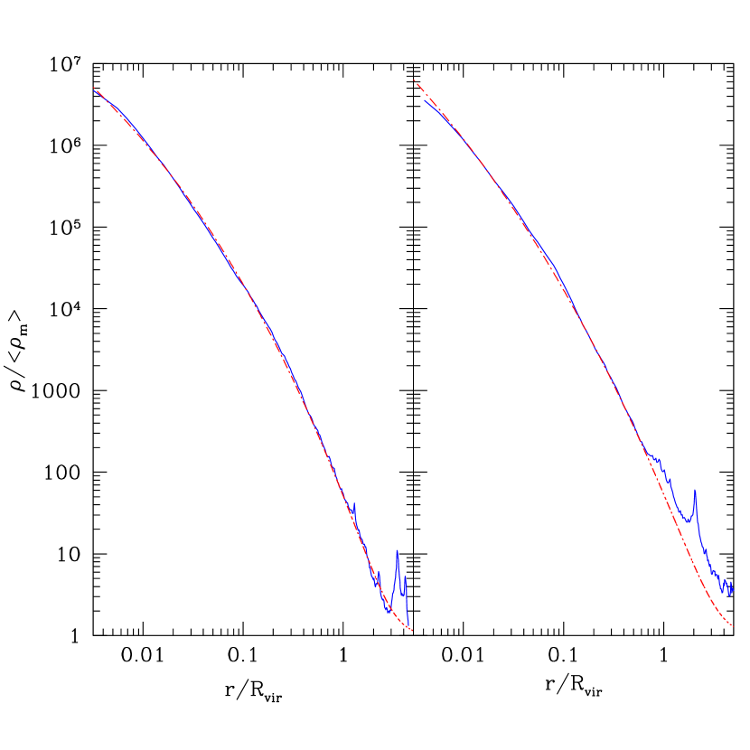
Figure 1: Dark matter density profiles of two dark matter halos (full curves) in the simulation Box20. The halos have virial masses of $1.4\times 10^{12}\mbox{$h^{-1}M_{\odot}$}$ (left panel) and $2.6\times 10^{11}\mbox{$h^{-1}M_{\odot}$}$ (right panel). The larger halo has a neighbour at 3.5 R_vir which is the halo on the right panel. This smaller halo is responsible for the spike at large radii in the density profile. In turn, the halo on the right panel has its own smaller neigbour at 2R_vir observed as a spike and an extended bump in the density profile. The dashed curves show the 3D Sersic profiles. The halo density profiles extend well beyond the formal virial radius with the Sérsic profile providing remarkably good fits.

Figure 2 gives more information on the structure of these two halos. The 3D rms velocities are what one would naively expect for “normal” halos. The rms velocity first increases when we go from the center and reaches a maximum at some distance. The radius of the maximum rms velocity is smaller for the halo on the right panel. This is because it has larger concentration. At larger radii the rms velocity first declines relatively smoothly. It has some fluctuations due to substructure. At radii larger than R_vir the decline stops. The average radial velocity is more interesting and to some degree is surprising. Nothing unusual inside R_vir: it is practically zero with tiny ($\approx 5\mbox{km~{}s${}^{-1}$}$) variations due to substructure. This is a clear sign of a virialized object. At larger distances the fluctuations in the velocity increase, but not dramatically if we compare those fluctuations with the rms velocities. The smaller halo on the right has a narrow dip ($V_{\rm rad}\approx-20\mbox{km~{}s${}^{-1}$}$) at $1.2\mbox{R${}_{\rm vir}$}$ apparently due to a satellite, which is moving into the halo. The surprising result is what we do not find, i.e., there is no infall on the two halos. This may seem like a fluke. Indeed, halos must grow. Their mass must increase with time. In order for the mass to increase, there should be on average negative infall velocities just outside the virial radius. Yet, we do not find those. We will later see that these two halos are not flukes, but are typical examples for halos of this mass range. What is important at this stage is that the infall velocities outside of R_vir are very small. They are significantly smaller than the rms velocities. These small radial velocities indicate that halos may extend to radii significantly larger than their formal virial radii.

Figure 2: The top curves on each panel show the 3D rms velocities at different radii for the halos shown in Figure 1. The bottom curves show the average radial velocities. The radial velocities show that for isolated halos of Milky-Way size and smaller halos there is no infall velocities outside of formal virial radius.

The average density profiles of isolated halos of different masses are shown in Figure 3. The isolation criteria in this case is no massive satellite inside $2\mbox{R${}_{\rm vir}$}$ ($d=2,m=5$; see Sec 2). The smooth density profiles, which are extremely accurately fit by eq.( 2), extend from the smallest resolved radius all the way to 2R_vir. Parameters of the density fits are given in Table 2. Note that in order to reduce the range of variations along the y-axis, we plot density multiplied by $(r/\mbox{R${}_{\rm vir}$})^{2}$. The horizontal parts of the curves in this plots correspond to density declining as $\rho\propto r^{-2}$. The density profiles are well above the average density of the Universe throughout all the radii. Even at $5\mbox{R${}_{\rm vir}$}$ the average density profile is still 4-5 times larger than the mean density. The upturn at large radii tells us that the density declines less steep than $r^{-2}$.

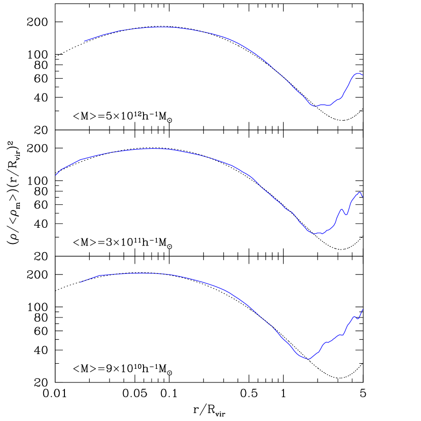
Figure 3: Average density profiles for halos with different virial masses. The 3D Sérsic profile provides very good fit with few percent errors within $2\mbox{R${}_{\rm vir}$}$. Even at $3\mbox{R${}_{\rm vir}$}$ the error is less than 20-30 percent. The density profiles are well above the average density of the Universe throughout all the radii.

The NFW approximation provides less accurate fits as shown in Figure 4. One may attribute the success of the 3D Sérsic approximation to the fact that it has three free parameters, while the NFW has only two. This is correct only to some degree. The problem with the NFW is that it has a slightly wrong shape at radii around $r_{s}$: its curvature is a bit too large. In Figure 4 this is manifested by an extended hump close to the maximum of the curves at $r\approx(0.05-0.2)\mbox{R${}_{\rm vir}$}$. One can shift the NFW slightly to the right and down to make the fit more accurate for most of the body of the halo ($r>0.05\mbox{R${}_{\rm vir}$}$). In this case the NFW fit goes below the halo density at small radii $r<0.05\mbox{R${}_{\rm vir}$}$, which sometimes was interpreted as if the central slope is steeper than -1. Overall, the 3D Sérsic approximation provides remarkable accurate fit. For $r=(0.01-2)\mbox{R${}_{\rm vir}$}$ the errors are smaller than 5%.

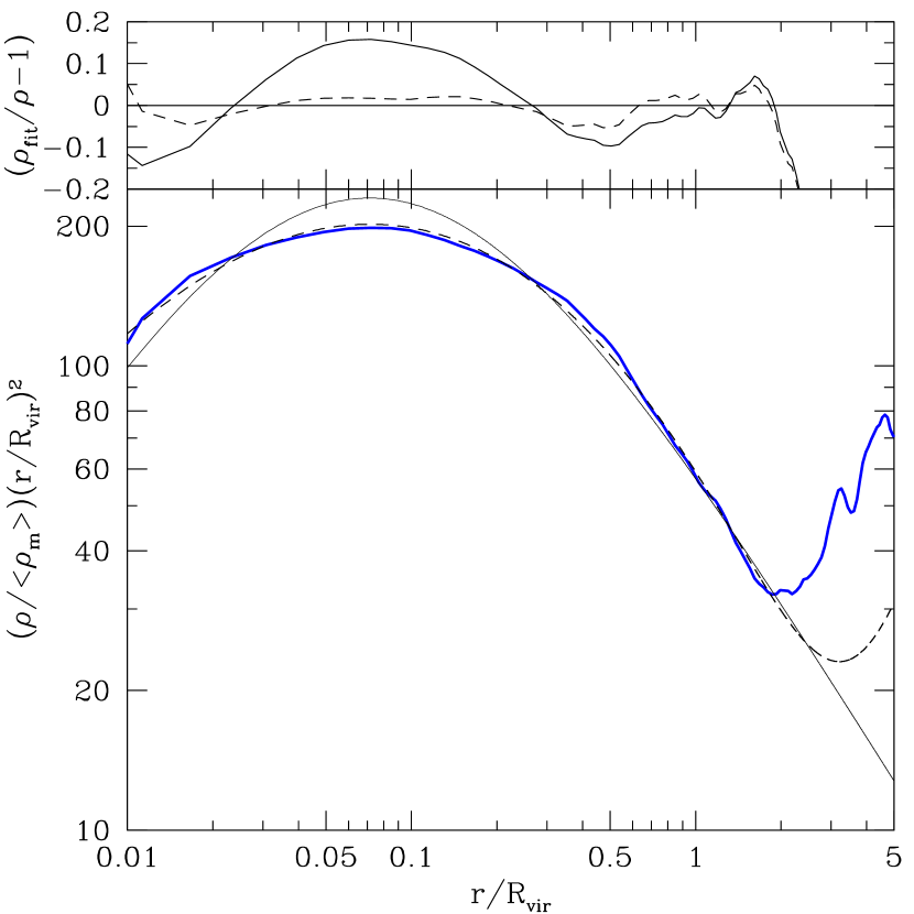
Figure 4: Comparison of the NFW and the 3D Sérsic fits. The thick full curve in the bottom panel shows the average density for halos with mass $<M>=3\times 10^{11}\mbox{$h^{-1}M_{\odot}$}$. The 3D Sérsic fit is the dashed curve. The NFW fit is presented by the thin full curve. The top panel shows the errors of the fits. The full curve is for the NFW approximation, and the dashed curve is for the 3D Sérsic fit. In outer regions $r=(0.3-2)\mbox{R${}_{\rm vir}$}$ both fits have practically the same accuracy. Both fits start to fail at larger distances. Overall, the 3D Sérsic approximation provides remarkable accurate fit.

Figure 5 shows how the density profile depends on particular choice of the isolation criterion. In this case we selected few hundred halos in the simulation Box80G with masses $M\approx 10^{12}\mbox{$h^{-1}M_{\odot}$}$. Qualitatively the same results are found for halos with different masses. Conclusions are clear: More strict isolation conditions result in smaller density in the outer parts of halos with almost no effect inside the virial radius. Even outside of the virial radius the difference are not that large. The difference between distinct (not isolated) halos and halos, which have no massive companions inside 2R_vir, are not more than a factor $\sim 1.5$. To large degree, this is not surprising because our isolated halos are typical, i.e., more that 1/2 of the halos in this mass range are “isolated”.

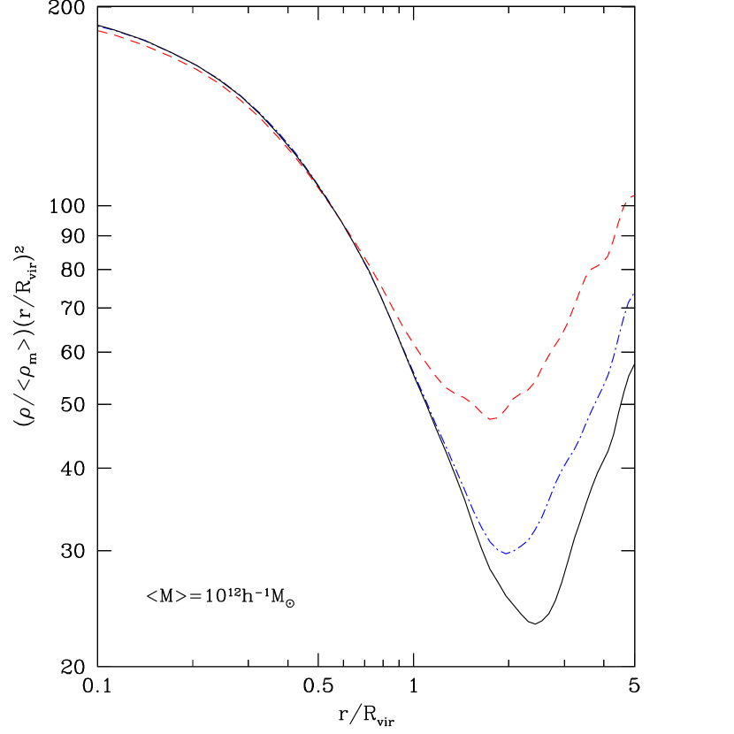
Figure 5: Effects of different isolation criteria on the density profiles. The dashed curve shows the average density profile of distinct halos with mass $M\approx 10^{12}\mbox{$h^{-1}M_{\odot}$}$ in Box80G. The dot-dashed and full curves are for isolated halos, which do not have massive companions inside $2\mbox{R${}_{\rm vir}$}$ and $3\mbox{R${}_{\rm vir}$}$ respectively. More strict isolation conditions result in lower density outside of the virial radius. At all shown radii the densities are well above the average density of the Universe.

One of the misconceptions, which we had before starting the analysis of the outer regions of dark matter halos is that at large distances the deviations from halo to halo are so large that it is very difficult to talk about average profile or a profile altogether. This appears to be not true. Figure 6 shows the halo to halo rms deviations from the average density profile for halos of a given mass. In order to construct the plot, we split the halo population into three ranges of concentrations and found the average and deviations for each concentration bin. Then the results of different concentrations were averaged. This splitting into concentrations is needed only for the central region $r<0.1\mbox{R${}_{\rm vir}$}$ because here the average profile depends on the concentration. This plot demonstrates that there is no drastic change in the deviations at the virial radius. The deviations increase with the distance, but they are not unreasonable.

Figure 6: RMS deviations of halo profiles from average profile for halos of given mass. The curves in the plot show results for halos with masses indicated in the plot. The deviations inside the formal virial radius are clearly smaller than for the outer regions. Inside the virial radius the deviations are smaller for halos with smaller mass.

Figure 7 shows the average radial velocity profile for halos of vastly different masses. We used many dozens of halos for each mass range. Just as in the case of the two individual halos in Figure 1 and 2, there is no systematic infall of material beyond formal virial radius for small virial masses. The situation is different for group- and cluster- sized halos (two top panels). For these large halos there are large infall velocities, which amplitude increases with halo mass.

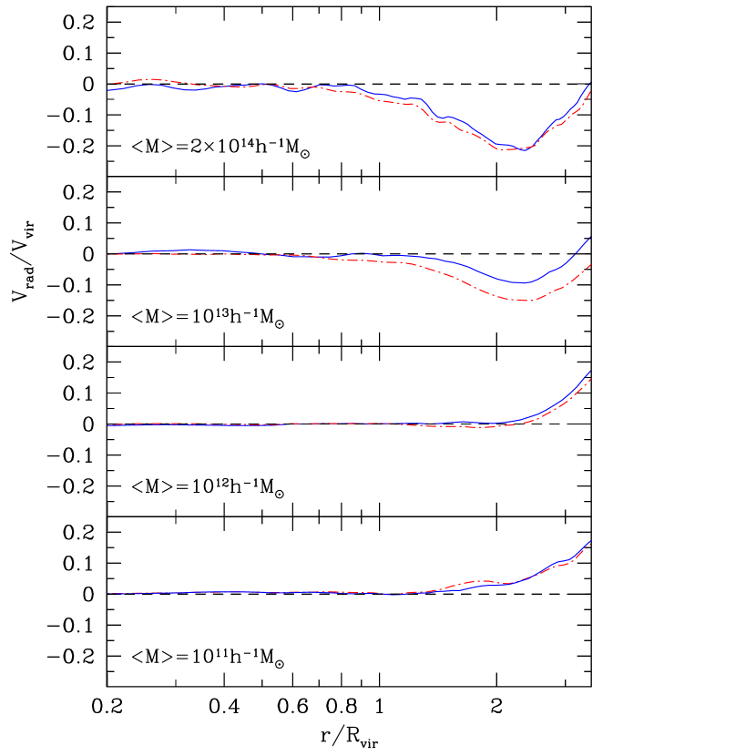
Figure 7: Average radial velocities for halos with different virial masses. The full curves show results for isolated halos and the dot-dashed curves are for distinct halos. The velocities are practically zero within $2-3~{}\mbox{R${}_{\rm vir}$}$ for halos with mass smaller than $10^{12}\mbox{$h^{-1}M_{\odot}$}$. The situation is different for group- and cluster- sized halos (two top panels). For these large halos there are large infall velocities, which amplitude increases with halo mass.

4 Predictions from the spherical collapse model

Here we obtain the predictions of the spherical collapse model (Gunn & Gott, 1972) for the $\it{mean}$ halo density profile and compare them with the results found in the numerical simulations. The spherical collapse model provides a relationship between the present nonlinear enclosed density contrast, $\delta=\langle\rho(r)\rangle/\langle\rho_{m}\rangle-1$, within a sphere of given radius $r$ and the enclosed linear density contrast, $\delta_{l}$, (i.e., the initial fluctuation extrapolated to the present using the linear theory) within the same sphere. This relationship along with the statistics of the initial fluctuations furnishes definite predictions for the mean density profile.

We expect the spherical collapse model to give the $\it{mean}$ density profile around virialized halos for sufficiently large radii - significantly larger than R_vir. In fact, for $r/\mbox{R${}_{\rm vir}$}>2.5$ we find a good agreement between the prediction of the spherical model and the $\it{mean}$ density profiles obtained from numerical simulations for several mass ranges. By $\it{mean}$ density profile we imply any representative profile for a given mass range. We consider three different representative profiles: the most probable profile, the mean profile and, what we call the typical profile. This last profile is simply the mean profile in the initial conditions spherically evolved.

Our procedure to obtain the typical density profile will be presented in full detail in Betancort-Rijo et al. (2005). In essence, we use the statistics of the initial Gaussian field to obtain the mean profile of the enclosed linear density contrast, $\delta_{l}(q)$, around a proto-halo as a function of the Lagrangian distance to the center, $q$. We then use the spherical collapse model to obtain the present density contrast, $\delta(r)$, as a function of the present comoving (i.e., Eulerian) distance to the center of the halo, $r$.

If $Q$ is the virial radius in Lagrangian coordinates, then the enclosed linear contrast $\delta_{l}(q,Q)$ must satisfy the condition that $\delta_{l}(q=Q)=\delta_{vir},$ where $\delta_{vir}$ is the linear density contrast within the virial radius R_vir at the moment of virialization. The present average enclosed fractional density $\delta(r=\mbox{R${}_{\rm vir}$})$ is equal to 340 (the value of overdensity $\Delta_{\rm vir}$ used in our simulations to define the virial radius). To obtain $\delta_{vir}$ we must find the $\delta_{l}$ corresponding to a present density contrast equal to 340. This condition leads to a $\delta_{vir}$ value of 1.9. We shall later comment on this once we introduce the spherical collapse model.

This condition simply ensures that the proto-halo evolves into an object which at present is virialized within the prescribed virial radius R_vir. If this were the only constraint on the linear profile (equal to the initial profile except for an overall factor), it have been shown (see Section 4 in Patiri et al. 2004) that:

$${\delta}_{l}(q,Q)\simeq\delta_{vir}\exp{\big{[}-b\big{(}\big{(}\frac{q}{Q}\big{)}^{2}-1\big{)}\big{]}}\equiv\delta_{0}(q,Q),$$ (3)

where $b$ is a coefficient depending on R_vir. It is given below.

However, although this profile does not lead to wrong results, in order to achieve the accuracy required here and to obtain the correct dependence of the shape on mass of the halos we must include an additional constraint. This constraint is:

$${\delta}_{l}(q,Q)<\delta_{vir}\quad\forall~{}q>Q.$$ (4)

It means that there are no radii larger than R_vir, where the density contrast is 340 or larger. Otherwise, the virial radius would be larger than R_vir. In the large mass limit this condition becomes irrelevant, and the linear density contrast is given by eq.(3). However, in the general case the mean linear profile, ${\delta}_{l}(q,Q)$, is somewhat steeper than $\delta_{0}(q,Q)$:

$$\delta_{l}(q,Q)=\delta_{0}(q,Q)-\frac{\sigma^{\prime}(q,Q)\exp[-x^{2}]}{1-\frac{1}{2}{\rm erfc}[-x]},$$ (5)

$$x\equiv\frac{\delta_{vir}-\delta_{0}(q,Q)}{\sqrt{2}\sigma^{\prime}(q,Q)}$$ (6)

with $\delta_{0}(q,Q)$ given in eq.(3), and

$$\sigma^{\prime}(q,Q)\equiv\sqrt{\sigma^{2}(q)-\Big{(}\frac{\delta_{l}(q,Q)}{\delta_{vir}}\Big{)}^{2}\sigma^{2}(Q)},$$ (7)

where $\sigma(q)$ and $\sigma(Q)$ are the $rms$ linear density fluctuations in spheres with lagrangian radii $q$ and $Q$. We use $\sigma_{8}=0.9$ as in the simulations.

With these definitions we have for the previously defined function $b(\mbox{R${}_{\rm vir}$})$:

$$b(R_{\rm vir})=-\frac{1}{4}\frac{d{\rm ln}\sigma(Q)}{d{\rm ln}Q}\bigg{|}_{Q=R_{\rm vir}(340)^{1/3}}$$ (8)

Using the linear density contrast eq.(5-6) we can now obtain the nonlinear density contrast, $\delta(r)$. For any given radius $r$ the nonlinear density contrast $\delta(r)$ is given by the solution to the equation:

$$\delta_{l}(\delta(r))=\delta_{l}(q,Q),$$ (9)

$$q\equiv r(1+\delta(r))^{1/3}\quad,\quad Q\equiv R_{vir}(340)^{1/3}.$$ (10)

The derivation of this eq.(9) may be found in Patiri et al.(2004), although here the equation is presented in a slightly different form. The left hand side of this equation is simply the relationship, $\delta_{l}(\delta)$, between the present and the linear $\delta$ value in the spherical collapse model (see Sheth & Tormen 2002) evaluated at $\delta=\delta(r)$. For the cosmology considered here we have for $\delta_{l}(\delta)$:

$$\delta_{l}(\delta) = \frac{1.676}{1.68647}\left[1.68647-\frac{1.35}{(1+\delta)^{2/3}}\right.$$ (11)

$$- \frac{1.12431}{(1+\delta)^{1/2}}+\left.\frac{0.78785}{(1+\delta)^{0.58661}}\right].$$

The right hand side of eq.(9), which depends on $\delta(r)$ through $q$, is given by expression (3).

Inserting eq.(5-6) into eq.(9) with $\delta_{vir}=1.9$, using for $b$ the values 0.186 and 0.254 for the two masses $6.5\times 10^{10}\mbox{$h^{-1}M_{\odot}$}$ and $3\times 10^{12}\mbox{$h^{-1}M_{\odot}$}$ discussed here, and solving for $\delta(r)$, we obtain the profiles for the present enclosed density contrast, $\delta(r)$. To obtain the density $\delta^{\prime}(r)$ at a given radius $r$ we simply need to take a derivative:

$$(1+\delta^{\prime}(r))\equiv\frac{\rho(r)}{\langle\rho_{m}\rangle}\quad,\quad\delta^{\prime}(r)=\frac{1}{3}\frac{1}{r^{2}}\frac{d}{dr}r^{3}\delta(r),$$ (12)

where $\langle\rho_{m}\rangle$ is the mean matter density of the Universe.

We must now comment on the value of $\delta_{vir}$ that we use. If the standard spherical collapse model were valid down to the virial radius we could use expression (11) to obtain it:

$$\delta_{vir}=\delta_{l}(340)=1.614$$

However, we know that this is not true because bellow $\sim 2$ virial radius there is substantial amount of shell-crossing that render the mentioned model unappropiate. This causes $\delta$ to grow much more slowly with $\delta_{l}$, so that when $\delta$ takes the value 340, $\delta_{l}$ takes the value 1.9 (Betancort-Rijo et al., 2005).

To obtain the predictions for the most probable and mean profiles, the probability distribution, $P(\delta,s)$, for the value of $\delta$ at a given dimensionless radius $s\equiv r/R_{vir}$ is needed. This distribution is derived in Betancort-Rijo et al.(2005) along the same lines we have described for the the typical profile. Here we simply use it to compute the most probable, $\delta(s)_{\rm prob}$ profile which is is simply given by the value at which $P(\delta,s)$ has its maxima. The mean profile, $<\delta(s)>$ is obtained from:

$$<\delta(s)>=\int_{-1}^{\infty}P(\delta,s)d\delta.$$ (13)

In practice, since the approximation we use for $P(\delta,s)$ has an unduly long tail, we have to truncate it artificially. So, we only integrate up to a $\delta$ value where $P(\delta,s)$ has fallen to a twenty fifth of its maximum value. The results are presented in Figure 8, where we have computed, both for $\delta$ and for $\delta^{\prime}$, the most probable (squares) and mean (crosses) density profiles found in our simulations for two mass intervals with the mean values equal to the masses used in the theoretical derivation. We have taken $277$ halos in the mass range $(6.5\pm 1.5)\times 10^{10}\mbox{$h^{-1}M_{\odot}$}$ from $Box80S$ and $654$ halos in the mass range $(3\pm 1)\times 10^{12}\mbox{$h^{-1}M_{\odot}$}$ from $Box80G$. No isolation criteria was used. In Table 3 we list for the mean halo with mass $<M>=3\times 10^{12}\mbox{$h^{-1}M_{\odot}$}$ the estimations of the most probable and mean value of the density at different radii compare with that from the spherical collapse model for the most probable, the mean and the typical profiles.

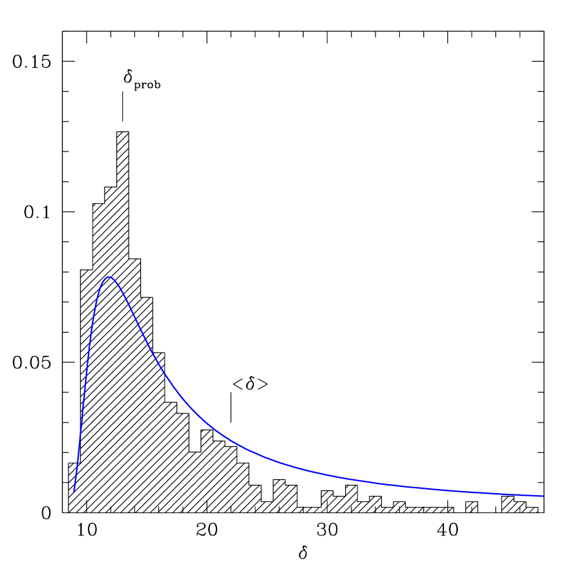
Figure 9: Distribution of the fractional cumulative density $\delta$ inside $3.5\pm 0.05\mbox{R${}_{\rm vir}$}$ for the mean halo of mass $<M>=3\times 10^{12}\mbox{$h^{-1}M_{\odot}$}$. We show for comparison the theoretical prediction of $P(\delta,s)$ as well as we give the most probable $\delta_{\rm max}$ and mean value $<\delta>$ of the distribution. We display the density distribution from its minimum value up to 1$\sigma$ from its mean $<\delta>$ (8% of the values of the distribution are beyond 1$\sigma$).

In Figure 8 one can see that beyond 2 virial radius the mean and the most probable profiles, both for $\delta$ and for $\delta^{\prime}$, differ considerably. This is due to the fact that for this radii the probability distribution for $\delta$, $P(\delta,s)$, is rather wide, with a long upper tail. This can be seen in Figure 9 were this distribution is shown inside $3.5\pm 0.05$ virial radius for the mass $<M>=3\times 10^{12}\mbox{$h^{-1}M_{\odot}$}$. We show for comparison the theoretical prediction for $P(\delta,s)$ as well as we give the most probable $\delta_{\rm max}$ and mean value $<\delta>$ of the distribution.

It is apparent from Figure 8 that the $\delta^{\prime}$ profiles are steeper for smaller masses, so that they go below the background at smaller $r/R_{vir}$ and reach larger underdensities. The $\delta$ profiles are also steeper for smaller masses although the difference is, obviously, much smaller. We have found that the theoretical prediction for the typical and the most probable profile are, in general, almost indistinguishable (see Table 3). They are both found to be in very good agreement with the most probable $\delta$ profile found in the numerical simulations beyond two virial radii. There is also qualitative agreement between the predictions of the most probable $\delta^{\prime}$ profiles and those found in the numerical simulations. It must be noted, however, that by predicted $\delta^{\prime}$ profile we understand simply the one obtained from the corresponding $\delta$ profile by means of relationship given in eq.(12). Note that this is not the same as the most probable profile for $\delta^{\prime}$ (see Figure 8). This is due to the fact that the most probable $\delta^{\prime}$ value at a given $s(\equiv r/R_{vir})$ corresponds to a different halo than the most probable $\delta$ value at the same $s$. This explains that, while the prediction for $\delta_{prob}$ agrees very well with the simulations, the agreement is not so good for $\delta^{\prime}_{prob}$. The $\delta^{\prime}_{prob}$ obtained from $\delta_{prob}$ by means of expression eq.(12) is not a proper prediction but an indicative value, since we can not envisage a feasible procedure to obtain a proper prediction. On the contrary, the mean profiles $<\delta>$ are exactly related to $<\delta^{\prime}>$ by means of expression eq.(12). The predictions for both profiles are in good agreement with the numerical simulations, showing a much flatter profile beyond 2 virial radius than those corresponding to $\delta_{\rm prob}$ and $\delta^{\prime}_{\rm prob}$. This agreement is remarkable given the fact that the expression used for $P(\delta,s)$ is only a first approximation (see Betancort-Rijo et al. 2005).

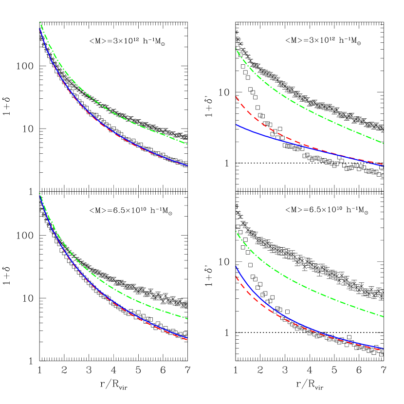
Figure 8: The most probable (squares) and the mean (crosses) halo density profiles up to 7R_vir for the two masses $(<M>=3\times 10^{12}\mbox{$h^{-1}M_{\odot}$}$ and $<M>=6.5\times 10^{10}\mbox{$h^{-1}M_{\odot}$}$ in our simulations. We compare the simulated data with the predictions from the spherical collapse model for the most probable (solid line) and typical profiles (dashed line) which are almost indistinguishable and the mean profiles (dot-short dashed line). We have estimated that the errors in the most probable values of $\delta$ and $\delta^{\prime}$ are about $25\%$ larger than the error showed in the plots for their mean values.

Table 3: Comparison between the simulated $\it{mean}$ halo density profile and the theoretical predictions from the spherical collapse model for the mass $<M>=3\times 10^{12}\mbox{$h^{-1}M_{\odot}$}$.

Numerical Simulations                            Spherical Collapse
$r/R_{\rm vir}$		$<\delta>$	$\delta_{\rm prob}$	$<\delta^{\prime}>$	$\delta^{\prime}_{\rm prob}$			$<\delta>$	$\delta_{\rm prob}$	$\delta_{\rm t}$	$<\delta^{\prime}>$	$\delta^{\prime}_{\rm prob}$	$\delta^{\prime}_{\rm t}$
1.0		337	323	69.1	52.4			531	398	385	40.4	2.5	7.8
1.5		129	116	30.8	15.1			184	115	118	22.6	1.9	4.3
2.0		67.7	54.6	19.5	3.73			84.8	53.7	51.7	14.7	1.5	2.8
2.5		43.2	31.1	15.4	1.6			49.3	28.6	27.6	10.3	1.2	1.9
3.0		30.8	17.4	11.2	0.78			32.2	17.3	16.6	7.6	1.0	1.4
3.5		22.1	12.6	8.5	0.58			22.6	11.3	10.9	5.8	0.79	0.97
4.0		18.4	9.0	5.9	0.18			16.8	7.9	7.6	4.5	0.61	0.70
4.5		14.1	5.8	5.5	0.09			13.0	5.8	5.5	3.5	0.46	0.50
5.0		12.2	4.4	4.3	-0.08			10.4	4.3	4.1	2.7	0.32	0.34
5.5		9.4	3.5	3.3	-0.16			8.5	3.3	3.2	2.1	0.20	0.22
6.0		7.9	2.8	3.1	-0.17			7.1	2.5	2.5	1.6	0.09	0.12
6.5		6.8	2.1	2.5	-0.22			5.7	2.0	2.0	1.2	-0.008	0.03
7.0		6.2	1.6	1.9	-0.33			4.6	1.6	1.6	0.9	-0.10	-0.04

It is interesting to note, as we have previously pointed out, that larger masses have somewhat shallower profiles. In order to predict this trend correctly we must use the initial profile given by eq.(5-6). If we dropped the second constraint (that is given in eq.(4) and use in eq.(9) the initial profile given by eq.(3), which corresponds to high mass objects, the prediction would be the opposite. The reason for this being that, in this limit, the initial profile depend on mass only through $c$ which increases with increasing mass, thereby leading to steeper profiles for larger masses.

As we stated in the introduction, the computations of the $\it mean$ profiles (in fact, the typical profile) around halos has independently been made by Barkana (2004). He used the spherical model and, in principle, imposed on the initial profile the same constraint as we do. The computing procedure he followed was somewhat different involving some approximations. He do not give explicitly the equation defining the profile, so that accurate comparison with our results are not possible. Furthermore he used different values of $\delta_{vir}$, $\Delta_{vir}$. However, his results are in good qualitative agreement with our predictions for the typical profile.

We have so far considered randomly chosen halos, i.e. without isolation criteria. When halos are chosen according with an isolation criteria they differ from the randomly chosen ones in two respects. On the one hand, the probability distribution for $\delta$ at a given value of $s$ is narrower, so that most profiles cluster around the most probable one. Therefore, the difference between the mean and the most probable density profile becomes smaller. On the other hand, isolated profiles lay, on average, on somewhat more underdense environment than non-isolated ones, so that their most probable profiles are slightly steeper. Both effects may be seen by comparing Table 3 and Table 4 or the upper right pannel in Figure 8 with Figure 10 where we show the local density profile for the isolated mean halo density profile for the mass range $3\pm 1\times 10^{12}\mbox{$h^{-1}M_{\odot}$}$. In this mass range we have selected halos that do not have a companion with mass larger than 10% of the halo mass within $4\mbox{R${}_{\rm vir}$}$. In total there are $156$ halos, i.e. one quarter of all halos in this mass range.

Figure 10: The mean (crosses) and most probable values (squares) of the local density profile for the mean isolated dark matter halo with mass $<M>=3\times 10^{12}\mbox{$h^{-1}M_{\odot}$}$.

Table 4: The isolated $\it{mean}$ halo density profile for the mass $<M>=3\times 10^{12}\mbox{$h^{-1}M_{\odot}$}$. The symbols are the same as table 3.

$r/R_{\rm vir}$		$<\delta>$	$\delta_{\rm prob}$	$<\delta^{\prime}>$	$\delta^{\prime}_{\rm prob}$
1.0		336	323	56.1	52.4
1.5		119	119	15.1	14.4
2.0		55.4	65.6	5.5	4.2
2.5		30.1	29.4	3.1	1.4
3.0		18.5	18.2	1.8	0.36
3.5		12.3	11.0	1.4	0.14
4.0		8.5	7.0	1.7	-0.04
4.5		6.4	6.0	1.6	0.03
5.0		5.2	4.6	2.5	-0.14
5.5		4.5	2.9	1.8	0.12
6.0		3.9	2.7	1.4	-0.20
6.5		3.4	2.0	1.3	-0.34
7.0		3.0	1.5	1.3	-0.30

5 Conclusions and Discussions

We perform a detailed study of the density profiles of isolated galaxy-size dark matter halos in high resolution cosmological simulations. We devote careful consideration mainly to the halo outer structure beyond the formal virial radius R_vir. We find that the 3D Sérsic three-parameter approximation provides excellent good density fits for these dark matter halos up to 2-3R_vir. These profiles do not display an abrupt change of shape beyond the virial radius. The halo-to-halo rms deviations from the average profile for halos of a given mass show that there is no a drastic change in the deviations at the virial radius. We show that these density profiles differ considerably from the NFW density profile beyond 3R_vir where the density profile are slower than $r^{-2}$. This result must not be seen as a contradiction when is compared with the $r^{-3}$ NFW fall-off at large radii since we must remember that the NFW analytical formula was proposed and extensively tested to describe the structure of virialized dark matter halos within R_vir. Although surprising, it is customary, for example, to see that the weak lensing analysis is often done with the NFW fit extrapolated to distances well beyond R_vir, up to large distances of several virial radii (up to few Mpc). This approach may not be accurate enough given the results presented in this work.

We also find that the isolated galaxy-size halos display all the properties of relaxed objects up to 2-3R_vir. In addition to their relatively smooth density profiles seen at large radii, by studying halos average radial velocities, we find that there is no indication of systematic infall of material beyond the formal virial radius. The dark matter halos in this mass range do not grow as one naively may expect through a steady accretion of satellites, i.e., on average there is no mass infall. This is strikingly different for more massive halos, such as group- and cluster-sized halos which exhibit large infall velocities outside of the formal virial radius. For large halos the amplitude of the infall velocities increases with halo mass.

For larger radii beyond 2-3 formal virial radius we combine the statistics of the initial fluctuations with the spherical collapse model to obtain predictions of the mean halo density profiles for halos with different masses. We consider two possibilities: the most probable and the mean density profiles. We find that the most probable profile obtained from our simulations is in excellent agreement with the predictions from the spherical collapse model beyond 2-3 virial radius. For the mean density profile the predictions are not so accurate. This is due to the fact that the approximation, which we are using for the distribution of $\delta$ at a given radius, has an artificially long tail (we are presently working on a better approximation). Even so, the predictions are qualitatively good and quantitatively quite acceptable. We think that the discrepancies between the data and the predictions at radii smaller than 2-3 virial radii are due to the fact that these inner shells are affected by the shell-crossing. We hope that an appropiate treatment of this circunstance will lead to accurate predictions for all radii, so that the mean spherically averaged profiles may be understood in terms of the spherical collapse. We find the results presented here very encouraging in this respect and we are currently working along this line.

References

- Barkana (2004) Barkana, R., 2004, MNRAS, 347, 59
- Bartelmann (1996) Bartelmann, M., 1996, å, 313, 697
- Bartelmann & Schneider (2001) Bartelmann, M., & Schneider, P., 2001, Phys., Rep., 340, 291
- Betancort-Rijo et al. (2005) Betancort-Rijo,J., Prada, F., Sánchez-Conde, M. A., & Patiri, S., 2005, in preparation
- Brainerd (2004) Brainerd, T.G., 2004, astro-ph/0409381
- Broadhurst et al. (2004) Broadhurst et al. 2004, astro-ph/0409132
- Bullock et al. (2001) Bullock, J. S., Kolatt, T. S., Sigad, Y., Somerville, R. S., Kravtsov, A. V., Klypin, A. A., Primack, J. R., & Dekel, A., 2001, MNRAS, 321, 559
- Conroy et al. (2004) Conroy, C., Newman, J. A., Davis, M., Coil, A. L., Yan, R., Cooper, M. C., Gerke, B. F., Faber, S. M., & Koo, D. C., 2004, astro-ph/0409305
- Crone et al. (1994) Crone, M. M., Evrard, A. E., & Richstone, D. O. 1994, ApJ, 434, 402
- de Blok et al. (2003) de Blok, W. J. G., Bosma, A., & McGaugh, S., 2003, MNRAS, 340, 657
- Diemand et al. (2004) Diemand, J., Moore, B., & Stadel, J., 2004, astro-ph/0402267
- Dubinski & Carlberg (1991) Dubinski, J., & Carlberg, R. 1991, ApJ, 378, 496
- Eke et al. (2001) Eke, V. R., Navarro, J. F., Steinmetz, M., 2001, ApJ, 554, 114
- Jing & Suto (2000) Jing, Y., & Suto, Y., 2000, ApJ, 529, L69
- Flores & Primack (1994) Flores, R., & Primack, J., 1994, ApJ, 427, L1
- Frenk et al. (1988) Frenk, C. S., White, S. D. M., Davis, M., & Efstathiou, G. 1988, ApJ, 327, 507
- Fukushige & Makino (1997) Fukushige, T., & Makino, J., 1997 ApJ, 477, L9
- Fukushige & Makino (2001) Fukushige, T., & Makino, J., 2001, ApJ, 557, 533
- Fukushige et al. (2004) Fukushige, T., Kawai, A., & Makino, J., 2004, ApJ, 606, 625
- Ghigna et al. (2000) Ghigna, S., Moore, B., Governato, F., Lake, G., Quinn, T., & Stadel, J., 2000, ApJ, 544, 616
- Gunn & Gott (1972) Gunn, J. E., & Gott, J. R., 1972, ApJ, 176, 1
- Guzik & Seljak (2002) Guzik, J., & Seljak, U., 2002, MNRAS, 335, 311
- Hoekstra et al. (2004) Hoekstra, H., Yee, H. K. C., Gladders, M. D., 2004, ApJ, 606, 67
- Keeton et al. (1998) Keeton, C. R., Kochanek, C. S., & Falco, E. E. 1998, ApJ, 509, 561
- Keeton (2001) Keeton, C. R. 2001, ApJ, 561, 46
- Klypin et al. (2001) Klypin, A., Kravtsov, A. V., Bullock, J. S., Primack, J. R., 2001, ApJ, 554, 903
- Klypin et al. (1999) Klypin, A., Kravtsov, A. V., Valenzuela, O., & Prada, F. 1999, ApJ, 522, 82
- Kneib et al. (2003) Kneib, J.-P. et al., 2003, ApJ, 598, 804
- Kravtsov et al. (1997) Kravtsov, A.V., Klypin, A.A., & Khokhlov, A.M., 1997, ApJS, 111, 73
- Mellier (1999) Mellier, Y. 1999, ARA&A, 37, 127
- Merritt et al. (2005) Merritt, D., Navarro, J. F., Ludlow, A., & Jenkins, A. 2005, ApJ, 624, L85
- Moore (1994) Moore, B., 1994, Nature, 370, 629
- Moore et al. (1998) Moore, B., Governato, Quinn, T., Stadel, J., & Lake, G. 1998, ApJ, 499, L5
- Navarro, Frenk, & White (1997) Navarro,J. F., Frenk, C. S., & White, S. D. M., 1997, ApJ, 490, 493
- Navarro et al. (2004) Navarro,J. F., Hayashi, E., Power, C., Jenkins, A., Frenk, C. S., White, S. D. M., Springel, V., Stadel, J., & Quinn, T.R., 2004, MNRAS, 349, 1039
- Patiri et al. (2004) Patiri, S., Betancort-Rijo, J., & Prada, F., 2004, astro-ph/0407513
- Prada et al. (2003) Prada, F., Vitvitska, M., Klypin, A., Holtzman, J. A., Schlegel, D. J., Grebel, E. K., Rix, H.-W., Brinkmann, J., McKay, T. A., & Csabai, I., 2003, ApJ, 598, 260
- Quinn et al. (1986) Quinn, P. J., Salmon, J. K., & Zurek, W. H. 1986, Nature, 322, 329
- Reed et al. (2003) Reed, D., Governato, F., Verde, L., Gardner, J., Quinn, T., Stadel, J., Merrit, D., & Lake, G., 2003, astro-ph/0312544
- Rhee et al. (2003) Rhee, G., Klypin, A. A., Valenzuela, O., Holtzman, J.K., & Moorthey, B., 2003, astro-ph/0311020
- Sheth & Tormen (2002) Sheth, R.K., & Tormen, G., 2002, MNRAS, 329, 61
- Sheldon et al. (2004) Sheldon, E. S., et al., 2004, AJ, 127, 2544
- Smith et al. (2001) Smith, D. R., Bernstein, G. M., Fischer, P., & Jarvis, M., 2001, ApJ, 551, 643
- Swaters et al. (2003) Swaters, R.A., Madore, B.F., van den Bosch, F.C., & Balcells, M., 2003, ApJ, 583, 732
- Tasitsiomi et al. (2004) Tasitsiomi, A., Kravtsov, A.V., Gottloeber, S., & Klypin, A.A., 2003, ApJ, 607, 125
- Warren et al. (1992) Warren, S. W., Quinn, P. J., Salmon, J. K., & Zurek, H. W. 1992, ApJ, 399, 405
- Wambsganss et al. (2004) Wambsganss, J., Bode, P., & Ostriker, J.P., 2004, ApJ, 606, L93
- Wechsler et al. (2002) Wechsler, R., Bullock, J., Primack, J., Kravtsov, A., & Dekel, A., 2002, ApJ, 568, 52
- Zaritsky & White (1994) Zaritsky, D. & White, S. D. M. 1994, ApJ, 435, 599
- Zaritsky et al. (1997) Zaritsky, D., Smith, R., Frenk, C., & White, S. D. M. 1997, ApJ, 478, 39
- Zhao et al. (2003) Zhao, D. H., Mo, H.J., Jing, Y.P., & Boerner, G., 2003, MNRAS, 339, 12