An Analysis of the Shapes of Ultraviolet Extinction Curves. IV. Extinction without Standards
(To appear in the September 2005 Astronomical Journal)

Abstract

In this paper we present a new method for deriving UV-through-IR extinction curves, based on the use of stellar atmosphere models to provide estimates of the intrinsic (i.e., unreddened) stellar spectral energy distributions (SEDs), rather than unreddened (or lightly reddened) standard stars. We show that this “extinction-without-standards” technique greatly increases the accuracy of the derived extinction curves and allows realistic estimations of the uncertainties. An additional benefit of the technique is that it simultaneously determines the fundamental properties of the reddened stars themselves, making the procedure valuable for both stellar and interstellar studies. Given the physical limitations of the models we currently employ, the technique is limited to main sequence and mildly-evolved B stars. However, in principle, it can be adapted to any class of star for which accurate model SEDs are available and for which the signatures of interstellar reddening can be distinguished from those of the stellar parameters. We demonstrate how the extinction-without-standards curves make it possible to: 1) study the uniformity of curves in localized spatial regions with unprecedented precision; 2) determine the relationships between different aspects of curve morphology; 3) produce high quality extinction curves from low color excess sightlines; and 4) derive reliable extinction curves for mid-late B stars, thereby increasing spatial coverage and allowing the study of extinction in open clusters and associations dominated by such stars. The application of this technique to the available database of UV-through-IR SEDs, and to future observations, will provide valuable constraints on the nature of interstellar grains and on the processes which modify them, and will enhance our ability to remove the multi-wavelength effects of extinction from astronomical energy distributions.

1 INTRODUCTION

A detailed determination of the wavelength dependence of interstellar extinction, i.e., the absorption and scattering of light by dust grains, is important for two very different reasons. First, since it is a product of the optical properties of dust grains, extinction provides critical diagnostic information about interstellar grain populations (including size distribution, grain structure, and composition), providing guidance for interstellar grain models. Second, the accuracy to which the intrinsic spectral energy distributions (SEDs) of most astronomical objects can be determined depends on how well the effects of extinction can be removed from observations. In both cases, a fundamental issue is how accurately the wavelength dependence of extinction can be measured. Consequently, it is essential to have a firm grasp of how measurement errors can affect the determination of this wavelength dependence.

This paper is the culmination of a series of “techniques” papers published over the past five years (Fitzpatrick & Massa 1999; Massa & Fitzpatrick 2000; and Fitzpatrick & Massa 2005; hereafter FM99, MF00, and FM05, respectively) whose aim has been to develop a technique to simultaneously determine the wavelength dependence of extinction (to higher accuracy than previously possible) and the physical properties of a reddened star. It represents a continuation of our earlier series on the properties of UV extinction (Fitzpatrick & Massa 1986; 1988; and 1990, hereafter FM90), and provides a detailed description of a new technique for deriving interstellar extinction curves which does not rely on observations of standard stars, virtually eliminates the effects of “mismatch” error, and yields an accurate assessment of the uncertainties. This “extinction-without-standards” technique opens the door to a new class of extinction studies, including regions heretofore inaccessible. For example, errors in the traditional “pair method” approach to extinction strongly limit our ability to study extinction in two important regimes. The first is low-$E(B-V)$ sightlines, where one might hope to relate extinction properties to the environmental properties of specific physical regions. The second is extinction derived from mid- to late B stars. These stars are plentiful, and often constitute the bulk of the stars available for extinction measurements in intrinsically interesting regions, such as the Pleiades. We will demonstrate how the extinction-without-standards approach overcomes both of these problems and present examples of each. Some first results from this program were illustrated by Fitzpatrick (2004, hereafter F04). In addition to the extinction results, we will demonstrate that our approach simultaneously provides accurate stellar parameters which are also astrophysically interesting.

In §2, we provide a broad overview of the basic problem of measuring an extinction curve, and compare the merits of curves derived by the pair method and curves derived by using stellar atmosphere models. In §3, we describe our new model-based technique in detail, and list the basic ingredients needed to determine an extinction curve using this approach. In §4, we describe the data used in the current study. In §5 we provide a number of sample extinction curves derived using model atmospheres. We also demonstrate the high precision of the new curves and the reliability of the error analysis employed. Finally in §6 we describe some to the scientific advantages of this new technique and our plans to exploit them.

2 MEASURING EXTINCTION

To understand how interstellar extinction is measured and to appreciate how different measurement techniques can affect the outcome, we begin with the intrinsic elements of an uncalibrated observation of a spectral energy distribution (SED) of a reddened star obtained at the earth, $f_{\lambda}$. This can be expressed as

$$f_{\lambda}=F_{\lambda}\,r_{\lambda}\,\theta_{R}^{2}\,10^{-0.4A_{\lambda}}$$ (1)

where $F_{\lambda}$ is the intrinsic surface flux of the star at wavelength $\lambda$, $r_{\lambda}$ is the response function of the instrument, $\theta_{R}\equiv(R/d)^{2}$ is the angular radius of the star (where $d$ is the stellar distance and $R$ is the stellar radius), and $A_{\lambda}$ is the absolute attenuation of the stellar flux by intervening dust (i.e., the total extinction) at $\lambda$. Alternatively, the observed SED can be expressed in terms of magnitudes $m_{\lambda}$ by

$$m_{\lambda} = -2.5\log F_{\lambda}\theta_{R}^{2}+A_{\lambda}+C_{\lambda}\;\;\;\;\;\;{\rm or}$$ (2)

$$m_{\lambda} = M_{\lambda}+5\log d-5+A_{\lambda}+C_{\lambda}$$ (3)

where $C_{\lambda}=-2.5\log r_{\lambda}$ is a term which transforms between the observed magnitude system and absolute flux units, and $M_{\lambda}$ is the traditional definition of the absolute magnitude of the star at $\lambda$.

The difficulty in measuring the total extinction $A_{\lambda}$ can be seen by rearranging these equations to solve for the extinction term. Equation 1 yields

$$A_{\lambda}=2.5\log(r_{\lambda}\theta_{R}^{2}\frac{F_{\lambda}}{f_{\lambda}})\;\;\;\;\;\;,$$ (4)

while Equation 3 yields

$$A_{\lambda}=m_{\lambda}-M_{\lambda}-5\log d+5+C_{\lambda}\;\;\;\;\;\;.$$ (5)

In either case, a true measurement of $A_{\lambda}$ would require calibrated SED observations, knowledge of the intrinsic SED of the star, and measurements of both the stellar distance and radius, or their ratio $\theta_{R}$. Unfortunately, there are no early-type stars for which both of these latter quantities are known to sufficient accuracy to allow a meaningful measurement of $A_{\lambda}$. As a result, indirect methods must be employed, and $A_{\lambda}$ is always a derived quantity, subject to assumptions.

In virtually all extinction studies, the actual measured quantity is a “color excess” which describes the extinction at a wavelength $\lambda$ relative to that at a fiducial wavelength. The traditional approach is to adopt the $V$ band as the fiducial, since $V$ magnitudes are widely available, accurately calibrated, and typically of high quality. This color excess can be expressed as either

$$E(\lambda-V)\equiv A_{\lambda}-A_{V}=2.5\log(\frac{r_{\lambda}}{r_{V}}\frac{F_{\lambda}}{F_{V}}\frac{f_{V}}{f_{\lambda}})\;\;\;\;\;\;,$$ (6)

as based on Equation 4, or

$$E(\lambda-V) \equiv A_{\lambda}-A_{V}$$ (7)

$$= (m_{\lambda}-m_{V})-(M_{\lambda}-M_{V})+(C_{\lambda}-C_{V})$$

$$= m(\lambda-V)-M(\lambda-V)+C(\lambda-V)\;\;\;\;\;\;,$$

as based on equation 5. Thus, the determination of the color excess requires only the measurement of the observed SED and a knowledge of the shape of the intrinsic SED. There are two basic approaches to determining color excesses, based on the use of either unreddened stars or stellar atmosphere models to represent the intrinsic SEDs of reddened stars. These two techniques, and the issue of the normalization of extinction curves, are discussed in the three subsections to follow.

2.1 The Pair Method

The first approach is the “pair method.” A pair method curve is constructed by comparing the fluxes of a reddened star and an (ideally) identical unreddened “standard star.” Essentially, the absolute magnitudes in Eq. 7 are replaced by the observed magnitudes of the standard star and the curve is usually expressed in the form

$$k(\lambda-V)\equiv\frac{E(\lambda-V)}{E(B-V)}\equiv\frac{m(\lambda-V)-m(\lambda-V)_{0}}{(B-V)-(B-V)_{0}}\;\;\;\;\;\;,$$ (8)

where the color excesses $E(\lambda-V)$ are normalized by $E$(B V) and the subscripted quantities refer to unreddened indices for the standard star. (The issue of normalization will be discussed below.) When the two stars are observed using the same instrument, this method has the advantage that calibration terms cancel, eliminating any dependence on the absolute flux calibration, $r_{\lambda}$ or $C_{\lambda}$. There are, however, two disadvantages to this technique. The first is that the grid of unreddened standard stars is necessarily limited, so that some mismatch in the SEDs of the reddened and unreddened stars, termed “mismatch error”, is inevitable. The second is that there are very few truly unreddened early-type stars, so usually the “unreddened” standard must be corrected for some small amount of extinction whose exact magnitude and wavelength dependence are uncertain. This creates an error that can propagate into the resulting extinction curves.

Massa, Savage, & Fitzpatrick (1983) presented a detailed study of the uncertainties affecting pair method extinction curves and showed that mismatch effects dominate the error budget. If one uses a single unreddened spectral standard for each spectral class, and assumes that all spectral classifications are perfect, then as a result of spectral binning, mismatch errors will be equal to or less than half a spectral class. Figure 1 shows how such mismatches can affect extinction curves derived from main sequence B stars. In each of the four groups of curves in Figure 1, the true shape of an extinction curve affecting a B1, B2, B5, or B9 star is indicated by the solid curve. The extinction curves which would be derived via the pair method in the presence of a $\pm\frac{1}{2}$ spectral class mismatch error are shown by the dash-dot curves for the case of $E(B-V)=0.15$ and by the dashed curves for $E(B-V)=0.30$. (The derived curves fall below the true curve in the UV and above the true curve in the IR when the standard star is cooler than the reddened star, and vice versa.) In practice, spectral classifications are not perfect and the available unreddened standard stars do not necessarily lie in the middle of the range of properties within a single spectral class. Both these effects exacerbate the spectral mismatch problem and thus the uncertainties shown in Figure  1 are likely closer to typical errors, rather than extremes.

Although it may appear from Figure 1 that a discontinuity at the Balmer jump at $\lambda^{-1}\simeq 2.7\mu{\rm m}^{-1}$ would provide an obvious indicator of the presence of spectral mismatch in an extinction curve, this is almost never practical. The spectrophotometric data available for constructing extinction curves are generally limited to UV wavelengths ($\lambda^{-1}>3.3\mu{\rm m}^{-1}$), which are highlighted in Figure 1. Typically, the only data available in the optical and near-UV are photometric indices which straddle the Balmer jump, such as the Johnson $U-B$ color, and these cannot be used to distinguish the effects of mismatch from intrinsic curve shape.

Mismatch error clearly can have a profound effect on the shapes of curves derived from stars with low color excesses, particularly in the mid-to-late B spectral range and most particularly in the UV spectral region. In fact, it is mismatch error which provides the low temperature cutoff to the spectral range of stars from which useful UV extinction measurements can be made. Mismatch also severely limits extinction studies based on stars hotter and/or more luminous than the main sequence B stars. For the O stars, very few unreddened standard stars exist and extreme mismatching of spectral types is often necessary to derive a curve — although, since the intrinsic UV/optical SEDs of the O stars are not well known, it is not clear how large an effect this introduces in the derived curves. The use of luminous, evolved stars for extinction studies is particularly problematic since unreddened standards are rare and the sensitivity of the intrinsic SEDs to both temperature and surface gravity can lead to very severe mismatch effects in the resultant curves (although see the discussion in Cardelli, Sembach, & Mathis 1992 for results in the early-B spectral range).

2.2 Model Atmosphere Techniques

The second approach to deriving extinction curves is to model the intrinsic SED of the reddened star in order to isolate the effects of extinction. This technique was first used by Whiteoak (1966) to analyze optical spectrophotometry and has been applied in one form or another many times since. We refer to it as “extinction-without-standards”, since it does not rely upon a set of unreddened standard stars to determine the extinction curve. In this method, a model atmosphere of the reddened star is determined from its photometric or spectral properties. The advantage of this approach is that, in principle, a perfect, unreddened match can be determined for the intrinsic SED of the reddened star, eliminating the mismatch error which plagues pair method curves. The apparent disadvantages of the approach are not actual disadvantages, but rather requirements, which can limit its accuracy and range of applicability. The first requirement is that a set of models must exist whose accuracy can be quantified and validated. The second is that the observations must contain adequate “reddening free” information to accurately determine the intrinsic SED of a reddened star. The third is that the fluxes must be precisely calibrated, i.e., $r_{\lambda}$ must well determined.

We have been developing the necessary constituents of this method over the past five years. We began by demonstrating that the Kurucz (1991) ATLAS9 models provide faithful representations of the observed UV and optical SEDs of near main sequence B stars (FM99). We then showed that a combination of an observed UV SED and optical photometry provides adequate reddening independent information to determine both the appropriate ATLAS9 model for a reddened star and a set of parameters (defined by FM90) which determine the shape of its interstellar extinction curve. Subsequently, we refined the calibration of the IUE data, in order to improve the quality of the fits and the robustness of the physical information derived from them (MF00). Next, we verified the physical parameters derived from the models through applications of the models to eclipsing binary data, where the results must agree with other constraints (see, Fitzpatrick et al. 2003 and references therein). Finally, we have used Hipparcos data of unreddened B stars to derive a consistent recalibration of optical and NIR photometry (FM05) and, in the process, once again demonstrated the internal consistency of the models for near main sequence B stars. As a result of these efforts, we now have internally consistent $r_{\lambda}$ for IUE and optical and NIR photometry, and are in a position to apply the results and to quantify the associated errors. These are the objectives of the current paper, and are discussed fully in the next section.

2.3 Normalizing The Curves

Once color excesses have been determined, we are faced with the problem of how to compare excesses derived for lines of sight with different amounts of extinction. After all, we are interested in the “shapes” of the curves, since these may reveal important clues about the size distribution and composition of the dust. This desire to compare shapes, brings us to the normalization problem.

From a purely mathematical point of view, a straightforward approach would be to normalize the curves by their norm,

$$e(\lambda-V)=\frac{E(\lambda-V)}{\sqrt{\sum_{\lambda}E(\lambda-V)^{2}}}$$ (9)

With appropriate weighting, this normalization could, on average, minimize the observational error in the normalization factor and reduce systematic effects. However, such a normalization would be sensitive to the strength of narrow features, such as the 2175Å bump, and this could mask the overall agreement between curves over the majority of the wavelength range. A second approach is to search for some immutable feature of the curve and normalize by that. The idea behind this procedure is that if some aspect of all curves is always the same, then all curves can be normalized by the strength of this property and all of the resulting curves will be directly comparable. This is the motivation for the $A_{V}$ normalization adopted by Cardelli, Clayton, & Mathis (1989). They assume that all extinction curves have a very similar (although not identical) form for $\lambda\gtrsim V$. However, there are problems with this normalization as well. In particular, as pointed out above, $A_{V}$ is not a directly measured quantity, but must be derived from IR photometry and requires assumptions about the shape of extinction curves at very long wavelengths. The shape of this extinction is often considered to have a universal form, but this has been demonstrated for only a relatively small number of sightlines (Reike & Lebofsky 1985; Martin & Whittet 1990). In addition, measurements of extinction in the IR can be compromised because the stellar SEDs become increasingly faint at long wavelengths and other sources of light, such as circumstellar emission or scattering from dust in the near stellar environment, can contaminate the SED measurements. Furthermore, IR color excesses are usually small for stars that are detectable in the UV, so UV curves normalized by quantities derived from IR photometry may be affected by large normalization errors. Consequently, the absolute level of such curves can be poorly defined. Finally, even with the advent of the 2MASS data base, there are still many stars which do not have IR photometry available.

As a result of the complications mentioned above, and since our intent is to demonstrate how precisely curves can be measured while making a minimum number of assumptions, we have opted to use the conventional $E(B-V)$ normalization, as shown in Eq. 8. While the interpretation of $E$(B V) as a measure of the “amount” of interstellar dust is not straightforward, its widespread availability, observational precision, and lack of requisite assumptions make it the best choice for this study. Nevertheless, we note that it is a simple matter to transform from one normalization to another, and emphasize that $E(\lambda-V)$ is actually the basic measurable quantity.

3 EXTINCTION-WITHOUT-STANDARDS

3.1 Formulation of the Problem

Our earlier studies (FM99, FM05) have shown that the observed SEDs, $f_{\lambda}$, of lightly- or unreddened main sequence B stars can be modeled very successfully by using a modified form of Eq. 1, namely,

$$f_{\lambda}=F_{\lambda}\,\theta_{R}^{2}\,10^{-0.4E(B-V)[k(\lambda-V)+R(V)]}\;\;.$$ (10)

The use of absolutely calibrated datasets eliminates the calibration term $r_{\lambda}$ and the total extinction $A_{\lambda}$ has been broken down into a normalized shape term ($k({\lambda-V})$), a normalized zeropoint ($R(V)\equiv A_{V}/$E$(\bv)$), and a scale factor ($E$(B V)). Providing that the righthand side of the equation can be represented in a parameterized form, the equation can be treated as a non-linear least squares problem and the optimal values of the parameters — which provide the best fit to the observed SED $f_{\lambda}$ — can be derived along with error estimates. Because the stars under study were lightly reddened, we could replace the extinction curve $k({\lambda-V})$ and the offset term $R(V)$ with average Galactic values without loss of accuracy. Using the Kurucz ATLAS9 stellar atmosphere models to represent $F_{\lambda}$, the results of the fitting procedure were estimates of 6 parameters: $E$(B V), $\theta_{R}$, and the four parameters that define the best-fitting model, i.e., $T_{\rm eff}$, $\log g$, the metallicity [m/H], and the microturbulence velocity $v_{t}$. We performed the fits using the MPFIT procedure developed by Craig Markwardt

The fitting process described above begins to break down when the color excess $E$(B V) of the target stars exceed $\sim$0.05 mag. By this we mean that large systematic residuals begin to appear, which greatly exceed the measurement errors. The reason is simple: the wavelength dependence of interstellar extinction curves varies greatly from sightline-to-sightline, and once $E(B-V)\gtrsim 0.05$ mag the differences between the true shapes of the curves and the assumed mean form begin to exceed the measurement error. However, FM99 noted that the SEDs of significantly reddened stars could still be modeled using Equation (10) (and the non-linear least squares approach) if the wavelength dependence of the extinction curve could be represented in a flexible form whose shape could be adjusted parametrically to achieve a best fit to the observations, and if these parameters were determined simultaneously with the stellar parameters. This is the essence of our “extinction-without-standards” approach.

Successfully modeling the shape of reddened stellar SEDs requires four principal ingredients: 1) an observed SED that spans as large a wavelength range as possible, 2) an accurate absolute flux calibration ($r_{\lambda}$ or $C_{\lambda}$), 3) an extinction curve whose shape can be described by a manageable set of parameters, and 4) a grid of stellar surface fluxes, $F_{\lambda}$, whose defining parameters can be determined from the observational data. In §4 we will describe the particular datasets used in this paper to demonstrate our technique. We have already discussed how MF00 and FM05 have determined the necessary calibrations. In the remainder of this section, we describe our flexible form for the interstellar extinction curve (§3.2) and the grid of stellar surface fluxes with which we have developed our approach (§3.3).

3.2 A Flexible Representation of the Interstellar Extinction Curve

We adopt a flexible and adjustable form for the UV-through-IR extinction curve, whose shape can be optimized to fit the SED of a reddened star through the adjustment of a specific set of parameters in the least-squares minimization procedure. This curve is illustrated in Figure 2. It consists of two main regions: 1) the UV ($\lambda<2700$ Å; solid curve) where the parameterized form of FM90 is adopted and 2) the near-UV/optical/IR ($\lambda>2700$ Å; dashed line) where we use a cubic spline interpolation through a set of UV (U₁, U₂), optical (O₁, O₂, O₃, O₄), and IR (I₁, I₂, I₃, I₄) anchor points to represent the curve. The interpolation is performed using the Interactive Data Language (IDL) procedure SPLINE. We adopt a spline representation for the near-UV/optical/IR curve simply because we do not have reliable, detailed information on the wavelength dependence of the extinction in the near-IR through near-UV region (1$\mu$m – 3000 Å). It is ironic that the portion of the curve that is accessible from the ground is more poorly characterized than the portion accessible only from space. As a result, we do not know whether the optical to near-IR region of the curve can be represented by a compact analytical formula. Our hope is that, by applying our procedure to a large sample of sightlines, we will ultimately be able to characterize the shape of the extinction law in this region by simple relations and determine whether sightline-to-sightline variations are correlated with other aspects of the curve or with interstellar environment. The placement of the spline points resulted from considerable experimentation, but certainly cannot be represented as an objectively determined optimal result. The current arrangement does, however, allow us to model the major available datasets to a level consistent with the observational errors.

The FM90 parameterization scheme contains 6 free parameters to represent 3 functionally separate features that are summed to produce the UV curve. An underlying linear component, indicated by the dotted line in Figure 2, is specified by an intercept $c_{1}$ and a slope $c_{2}$. The Lorentzian-like 2175 Å bump is fit by a Drude profile $D(x,x_{0},\gamma)$, where $x_{0}$ and $\gamma$ specify the position and FWHM of the bump, respectively, whose strength is determined by a scale factor $c_{3}$. Finally, the degree of departure of the curve in the far-UV from the underlying linear component is specified by a single parameter $c_{4}$. Defining $x\equiv\lambda^{-1}$, the complete UV function is given by:

$$k(\lambda-V)=c_{1}+c_{2}x+c_{3}D(x,x_{0},\gamma)+c_{4}F(x)\;\;,$$ (11)

where

$$D(x,x_{0},\gamma)=\frac{x^{2}}{(x^{2}-x_{0}^{2})^{2}+x^{2}\gamma^{2}}\;\;,$$ (12)

and

$$F(x;x>5.9) = 0.5392(x-5.9)^{2}+0.05644(x-5.9)^{3}\;\;,$$ (13)

$$F(x;x\leq 5.9) = 0\;\;.$$ (14)

It is worth emphasizing that the FM90 parameterization is a mathematical scheme only, which allows us to reproduce UV extinction curves in a shorthand form (and makes the current program possible). However, it is not to be assumed that the functional components of the scheme represent actual separate extinction components arising in distinct dust grain populations. This parameterization has proven very useful and to the best of our knowledge is able to reproduce all known UV extinction curves to the level of observational error. Its flexibility will be illustrated in §5 below. Note that we terminate the FM90 formula at 2700 Å, although we originally utilized UV data extending to 3000 Å. Additional experience with the UV data has suggested that real extinction curves begin to exhibit departures from the FM90 formula near 2700 Å, due to the unrealistic extrapolation of the linear component into the blue-violet region.

The 10 spline anchor points which characterize the near-UV/optical/IR portion of the curve are determined by a least squares fit to the IUE data longward of 2700 Å and the available optical and IR photometry. Although there are 10 anchor points, there are also 6 constraints, so the fit actually introduces only 4 additional degrees of freedom. We now discuss these constraints in detail.

The two UV anchor points, U₁ and U₂ at 2700 and 2600 Å, respectively, are fixed at the values of the FM90 UV fitting function at their wavelengths and are not adjustable. Together with O₁ at 3300Å, these points guarantee that the curve which passes through the IUE data between 2700 and 3000 Å will join both the UV and optical portions of the curve smoothly.

The four optical anchor points, O₁, O₂, O₃, and O₄ at 3300, 4000, 5530, and 7000 Å, respectively, are fit under two constraints: that the interpolated curve produces a value of $k(\lambda-V)=0$ in the V band, and that the curve be normalized to unity in $E$(B V). Thus, only two free parameters emerge from this region.

The four IR points, I₁, I₂, I₃, and I₄ are located at 0.25, 0.50, 0.75, and 1.0 $\mu$m^-1, respectively. These four points are constrained to satisfy the formula

$$I_{n}\equiv k(\lambda-V)=k_{IR}\lambda_{n}^{-1.84}-R(V)$$ (15)

where the scale factor, $k_{IR}$, and the intercept, $R(V)$, are the only free parameters. This is the power-law form usually attributed to IR extinction, with a value for its exponent from Martin & Whittet (1990). The exponent of the power-law could, potentially, be included as a free parameter in the fitting procedure, and we will investigate this in the future. However, our impression is that the IR data available to us (primarily 2MASS $JHK$ photometry) are insufficient to determine this quantity accurately. All results presented in this paper assume an exponent of -1.84 in Equation 15.

3.3 The Stellar Surface Fluxes

To represent the intrinsic surface fluxes, $F_{\lambda}$, of reddened stars we utilize R.L. Kurucz’s line-blanketed, hydrostatic, LTE, plane-parallel ATLAS9 models, computed in units of erg cm^-2 sec^-1 Å^-1 and the synthetic photometry derived from the models by Fitzpatrick & Massa (2005). These models are functions of four parameters: $T_{\rm eff}$, $\log g$, [m/H], and $v_{t}$. All of these parameters can be determined in the fitting process although, because of data quality, it is sometimes necessary to constrain one or more to a reasonable value and solve for the others.

The general technique of deriving extinction curves via stellar atmospheres is, of course, not dependent on the specific set of models used. In the present case, the most important consideration for our adoption of the ATLAS9 models is that they work — at least within a specific spectral domain. FM99 and FM05 have shown that these models provide excellent fits to the observed SEDs for lightly- or un-reddened main sequence B stars throughout the UV through near-IR spectral region. In addition, experience with eclipsing binaries (see Fitzpatrick et al. 2003 and references within) has shown that the good SED fits also yield accurate estimates of the physical properties of the stars. Because of the physical ingredients of the models (specifically LTE and plane-parallelism) we currently restrict our attention to the main sequence B stars. We plan to investigate how well these models reproduce the SEDs and properties of somewhat more luminous B stars and also the later O types. Also, we will take advantage of more complex models (e.g., the non-LTE TLUSTY models) as the available grids expand their parameter ranges.

3.4 Summary

To summarize, we model the observed SEDs of reddened near main sequence B stars by treating equation (10) as a non-linear least squares minimization problem. As a result we can simultaneously obtain estimates of the physical properties of a reddened star and the shape of the interstellar extinction curve distorting the star’s SED. A total of 16 parameters specify the righthand side of the equation, including $\theta_{R}$, $E(B-V)$, four to define $F_{\lambda}$, and ten to define the shape of the extinction curve. Depending on limitations of the available data, and known properties of the stars or interstellar medium, any subset of the parameters can be constrained to predetermined values.

4 THE DATA

In the following section, we will illustrate the potential of our extinction-without-standards technique, utilizing a set of 27 lightly-to-heavily reddened stars. For this demonstration, and indeed for extinction determinations in general, the ideal SED dataset would consist of absolutely-calibrated spectrophotometry spanning the UV-through-IR spectral regions. Such data would allow a straightforward comparison between observations and stellar atmosphere models (since both are presented in simple flux units) and would provide the most detailed view of the wavelength dependence of interstellar extinction. While a small amount of such data is available (see, e.g., Fitzpatrick at al. 2003), the largest existing database of absolutely-calibrated spectrophotometry is the low-resolution archive of the International Ultraviolet Explorer satellite (IUE) which covers the UV region only (1150–3000 Å). In the optical and near-IR, the largest SED databases are photometric in nature, consisting of Johnson, Strömgren, and Geneva photometry in the optical and 2MASS JHK photometry in the near IR. Utilizing these resources, we can examine the UV region for small scale features but can only study the broad scale wavelength-dependence of extinction in the optical and near-IR regions.

We use NEWSIPS IUE data (Nichols & Linsky 1996) obtained from the MAST archive at STScI. These data were corrected for residual systematic errors and placed onto the HST/FOS flux scale of Bohlin (1996) using the corrections and algorithms described by MF00. This step is absolutely essential for our program since our “comparison stars” are stellar atmosphere models and systematic errors in the absolute calibration of the data do not cancel out as in the case of the pair method. (The NEWSIPS database is also contaminated by thermally- and temporally-dependent errors, which would not generally cancel out in the pair method — see MF00.) Multiple spectra from each of IUE’s wavelength ranges (SWP or LWR and LWP) were combined using the NEWSIPS error arrays as weights. Small aperture data were scaled to the large aperture data and both trailed and point source data were included. Short and long wavelength data were joined at 1978 Å to form a complete spectrum covering the wavelength range $1150\leq\lambda\leq 3000$ Å. Data longward of 3000 Å were ignored because they are typically of low quality and subject to residual systematic effects. The IUE data were resampled to match the wavelength binning of the ATLAS9 model atmosphere calculations in the wavelength regions of interest.

Mean values of the Johnson UBV, Strömgren uvby$\beta$, and Geneva UBB₁B₂VV₁G photometric magnitudes, colors, and indices for the program stars were acquired from the Mermilliod et al. (1997) archive. 2MASS JHK magnitudes for all stars, along with their associated errors, were obtained from the 2MASS All-Sky Point Source Catalog at the NASA/IPAC Infrared Science Archive. Johnson $V-R$, $R-I$, and JHK data are also available for some of the stars, and were obtained from the Mermilliod et al. archive.

5 SOME INITIAL RESULTS

In this section, we demonstrate the potential of our extinction-without-standards technique, utilizing a set of the 27 reddened stars, listed in Table 1, which fall into three groups: 1) stars in the open cluster IC 4665; 2) stars with moderate-to-heavy reddening; and 3) lightly reddened stars in a specific region of the sky. These representative examples illustrate the advantages of our approach and highlight several scientific applications which will be pursed in future studies, using expanded samples of stars. In addition, they provide confirmation of the error analysis incorporated in our approach.

For this demonstration sample, the SED fitting procedure was applied as described above, with the following additional details:

• The SED data modeled in the fitting procedure include IUE UV spectrophotometry, the Johnson $V$, $B-V$, and $U-B$ indices, the Strömgren $b-y$, $m_{1}$, $c_{1}$, and $\beta$ indices, the Geneva $U-B$, $V-B$, $B_{1}-B$, $B_{2}-B$, $V_{1}-B$, and $G-B$ indices, and the 2MASS JHK magnitudes. Johnson $V-R$, $R-I$, and JHK data are also available for a few of the stars.

• The optical extinction spline point O₄ at 7000 Å is only well-determined when optical $R$ and $I$ band photometry are available. Therefore in the examples below, we only solve for O₄ in such cases. For the other stars, the optical portion of the extinction curve is determined only by the spline points O₁, O₂, and O₃.

• During the $\chi^{2}$ minimization, a reddened and distance-attenuated model was created from the current set of input parameters, and then synthetic photometry was performed on this model to produce the photometric indices, which were then compared with observations. The synthetic photometry was calibrated as described by FM05, with the calibration extended to redder colors by us. The UV model fluxes and recalibrated IUE fluxes, both in units of erg cm^-2 sec^-1 Å^-1, were compared directly.

• The initial weighting factors for the various datasets in the $\chi^{2}$ minimization were determined from their observational uncertainties, i.e., $weight\propto\sigma^{-2}$. We then scaled the weights of the optical/near-IR photometry so that their total weight was equal to that of the IUE UV spectrophotometry, thus balancing the fit between the two datasets. This is the procedure adopted by FM05, except that we include the Strömgren $\beta$ index along with the rest of the optical/near-IR photometry, rather than assigning it its own (high) weight. FM05 weighted $\beta$ heavily in recognition of its value as a surface gravity indicator. However, we have found that the temperature-sensitivity of $\beta$ (particularly in the later B stars) combined with observational errors, can lead to very unsatisfactory fits when $\beta$ is over-emphasized. Treating $\beta$ in the same manner as the rest of the photometric indices seems to be the simplest and most reasonable approach.

• Because interstellar H i Lyman $\alpha$ absorption in reddened stars can have a significant impact on the star’s apparent continuum level far from line center at 1215 Å, we convolve the profile of this heavily damped line with the model atmosphere SEDs before comparing with observations. Along heavily reddened sightlines, where the H i column density $N($H i$)$ is high and the signature of the atomic absorption strong, the value of $N($H i$)$ can actually be incorporated into the fitting procedure as a free parameter to be optimized. We will utilize this capability in future studies. For the present, mostly lightly-reddened, sample, however, the $N($H i$)$ values used to construct the line profiles were taken from the survey of Diplas & Savage (1994) or else computed from the general relation $N($H i$)=4.8\times 10^{21}E(B-V)\;{\rm cm}^{-2}$ from Bohlin, Savage, & Drake (1978). The inclusion of the Lyman $\alpha$ line insures that we distinguish the effects of dust extinction from atomic absorption in the far UV region.

• The uncertainties in the best-fit parameters were determined by running 50 Monte Carlo simulations for each star, during which the input data were randomly varied assuming a Gaussian distribution of observational uncertainties and a new fit performed. The zero points and random photometric uncertainties of the short-wavelength and long-wavelength IUE fluxes were varied as described in FM04; the assumed observational errors in the Johnson, Strömgren, and Geneva indices were as given in Table 7 of FM04; and the uncertainties in the 2MASS data were as obtained from the 2MASS archive. In addition, the $V$ magnitude was assumed to have a 1-$\sigma$ uncertainty of 0.015 mag. The adopted 1-$\sigma$ uncertainties for each parameter were taken as the standard deviation of the values produced by the 50 simulation.

5.1 The Open Cluster IC 4665

We begin our examples by examining the extinction towards an open cluster. While multiple scientific rewards can result from the study of extinction towards cluster stars (see the discussion in §6), our primary interest in IC 4665 is to demonstrate the “technical” advantages of our approach. Namely, the use of cluster extinction curves to help evaluate the magnitude of the uncertainties in the measurement of extinction curves, as discussed in detail by Massa & Fitzpatrick (1986). In particular, and because of its low $E(B-V)$ and late-B stellar population, IC 4665 extinction curves provide an especially sensitive test of the precision and range of our extinction-without-standards approach.

The wavelength dependence of extinction towards IC 4655 was first examined by Hackwell, Hecht, & Tapia (1991; hereafter HHT) for the purpose of studying the relationship between extinction and IR emission, as measured by the Infrared Astronomical Satellite (IRAS). This remains one of the most challenging extinction studies yet performed for two reasons: 1) the mean reddening in the cluster is very low, $\langle E(B-V)\rangle<0.2$ mag, and 2) the spectral types of the available targets run from mid- to late B. Both facts exacerbate errors in the standard pair method approach, as has been shown in Figure 1. HHT recognized these uncertainties and ultimately concluded that the wavelength dependence of extinction among the cluster stars is uniform to within their ability to measure it.

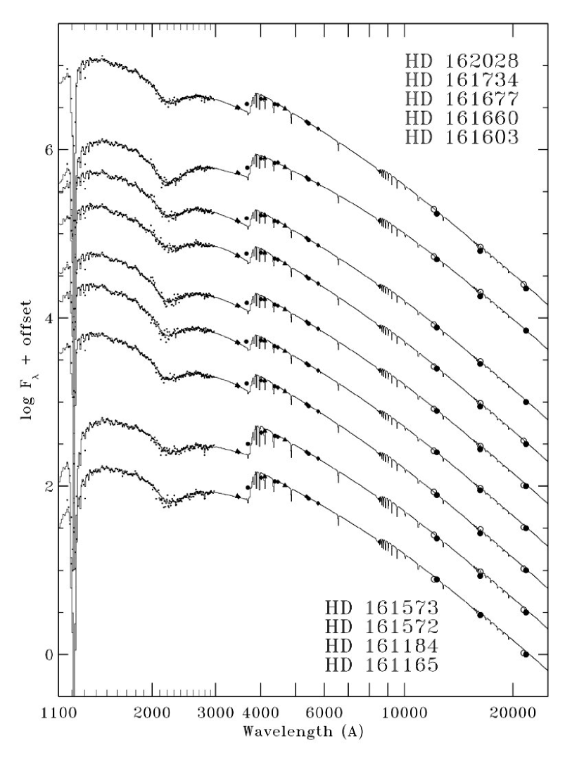
Figure 3: SED fits for nine lightly-reddened mid-to-late main sequence B stars in the open cluster IC 4665. Histogram-style curves are the best-fitting, reddened ATLAS9 stellar atmosphere models, arbitrarily shifted vertically for clarity. In the UV ($\lambda<3000$ Å), small filled circles are IUE low-dispersion spectrophotometry binned to match the resolution of the models. In the optical, circles, triangles, and diamonds are Johnson UBVRI, Stromgren uvb, and Geneva UB₁B₂VV₁G data, respectively. In the IR, the large open and closed circles are Johnson JHK and 2MASS JHK data, respectively. The photometric data have been converted to flux units for display purposes only. As discussed in §5, the comparison between models and photometric magnitudes, colors, and indices is performed in the native format of the photometry.

Figure 3 shows the results of the SED fits for the nine IC 4665 stars considered here. The SED’s of the best-fitting, reddened models are shown by the histogram-style curves. In the UV, the binned IUE fluxes are shown by the small circles. In the optical region, Johnson UBVRI magnitudes (converted to flux) are indicated by circles, Strömgren uvby magnitudes by triangles, and Geneva UB₁B₂VV₁G magnitudes by diamonds. In the near-IR, 2MASS and Johnson JHK magnitudes are shown by the large filled and open circles, respectively. Note that the photometric data have been converted to flux units for display purposes only. The comparison between models and observations was performed in the native photometric format (i.e., in magnitudes or colors as noted above).

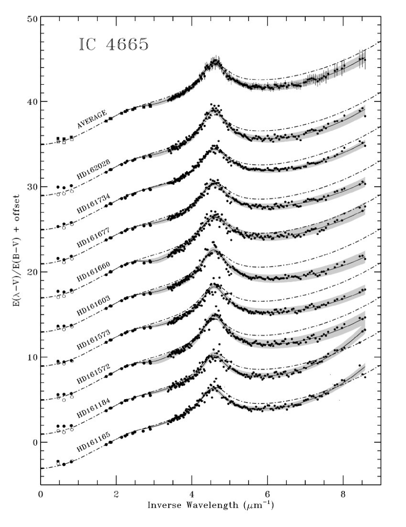
Figure 4: Extinction curves derived using model atmosphere calculations for nine mid-to-late B main sequence stars from the open cluster IC 4665. The values of $E(B-V)$ range from 0.14 to 0.25 for this group. The filled symbols show IUE spectrophotometry in the UV ($\lambda^{-1}>3.33\/\mu{\rm m}^{-1}$), Johnson, Stromgren, and Geneva photometry in the optical, and 2MASS JHK in the near-IR. Open symbols indicate near-IR Johnson JHK data. The solid curves are the fits to the data (i.e., the “flexible, parametrized curves” described in §3.2) as determined by the SED-fitting procedure, and the shaded regions show the 1-$\sigma$ uncertainty in the curves, based on Monte Carlo simulations. For comparison, the dash-dot curves show the average Galactic extinction curve (corresponding to $R(V)=3.1$). Because of an apparent conflict in the 2MASS and Johnson JHK data, we assumed that the shape of the IC 4665 curves in the near-IR follows the average Galactic curve. The top solid curve and the square symbols show the simple mean of the nine IC 4665 extinction curves, along with the average Galactic curve for comparison. The error bars indicate the sample standard deviation of the individual curves. Note that this scatter is comparable to the 1-$\sigma$ errors of the individual curves, indicating that the shape of the extinction curve in IC 4665 is uniform to within our (small) measurement errors.

Figure 4 shows our extinction-without-standards curves for the IC 4665 stars. The symbols show the actual normalized ratios between the models and the stellar SEDs, while the thick solid curves show the flexible UV-through-IR extinction curves whose shapes were determined by the fitting procedure. The curves have been arbitrarily shifted vertically for clarity, but all are shown compared with a similarly-shifted estimate of the average Galactic extinction curve for reference (thick dash-dot curves corresponding to $R(V)=3.1$, from Fitzpatrick 1999). As will be discussed further below, we assumed a value of $R(V)=3.1$ towards the cluster and did not include the IR JHK data in the fitting procedure. Thus, only the average Galactic curve is shown for wavelengths longward of 6000 Å.

The various parameters determined by the fits are listed in Tables 1 and 2. The flexible extinction curves themselves, in the form $E(\lambda-V)/E(B-V)$ can be reconstructed from the parameters given in Table 2. The 1-$\sigma$ uncertainties of the extinction curves are indicated in Figure 4 by the grey shaded regions. The regions are centered on the means of the 50 Monte Carlo simulations with which we performed our error analysis and their thickness shows the standard deviation of the individual simulations.

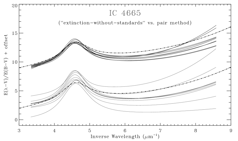
Figure 5: Comparison between extinction curves derived for the cluster IC 4665 using the extinction-without-standards technique described in this paper (upper set of curves) and using the traditional pair method approach (lower set of curves; from HHT). The average Galactic curve is shown with both sets of curves for reference (dash-dot curves).

Figure 5 compares our new curves in the UV with those derived by HHT using the standard pair method. HHT’s curves were reconstructed from the data in their Table 5. Note that the HHT study originally included 17 stars. We have eliminated 4 A-type stars, 3 chemically peculiar B-type stars, and 1 B-type shell system from consideration here since their extinction curves are particularly uncertain. Thus, Figures 4 and 5 show only the best-determined curves in the cluster, from the point of view of both the pair method and our technique. The remarkable aspect of Figure 5 is not the scatter among HHT’s curves — it is exactly what should be expected given the limitations of the pair method — but rather the impressive improvement in precision gained by the extinction-without-standards technique, as evidenced by the decrease in the curve-to-curve scatter. Clearly, this higher level of precision allows much firmer conclusions to be drawn about the degree of intrinsic variation of extinction across the face of the cluster, and also affords an improved potential to detect correlated behavior between the extinction properties and other aspects of the interstellar environment.

While we will present a full scientific analysis of the IC 4665 results in a future paper, the issue of the intrinsic variation of extinction among the cluster stars is important to consider here, since it can shed light on the accuracy of our error analysis. The top curve in Figure 4 shows the mean of the nine individual IC 4665 curves. The error bars show the actual sample standard deviation and the average Galactic curve is again presented for comparison. The critical result is that, over most of its wavelength range, the standard deviation of the sample about the mean curve is comparable to the predicted uncertainties in the individual curves, as shown by the shaded regions. This indicates that the (small) curve-to-curve variations seen are at a level consistent with our expected uncertainties and that the intrinsic level of variation among the cluster stars must be very low.

Another way to approach the issue of variability is to look at the scatter among the various parameters which define the extinction curves. These are shown in Table 3, where columns 2 and 3 list the weighted mean values of the parameters and their observed standard deviations, respectively. The predicted uncertainties, i.e., the RMS of the Monto Carlo-based errors for the individual stars, are listed in column 4. If our error analysis is reasonable, then the observed scatter should be the quadratic sum of the expected errors plus any intrinsic variability. The value of examining cluster extinction curves is that one might reasonably suppose (at least as a starting point) that the individual curves, derived for nearly coincident lines of sight, are actually independent measurements of a single “cluster curve,” i.e., no intrinsic scatter. In such a case, the measured scatter actually reflects the real measurement errors and provides an important test of the error analysis. Examination of Table 3 shows that the predicted and observed scatters are indeed generally very similar, supporting the position that any intrinsic variations among the IC 4665 curves are close to the level of our ability to measure them and that we have accurately assessed the uncertainties in our results. The final column of Table 3 shows the implied values of the possible small intrinsic variations.

Several of the individual parameters merit some additional comment. Both the 2175 Å bump FWHM ($\gamma$) and its strength ($c_{3}$ or $A_{bump}$) show evidence for some small level of variability within the sample, above our expected measurement errors. However, this is not clearcut because these measurements involve the region of the IUE spectra which typically has the lowest quality data and it is possible that weak systematic effects in the data themselves — which are not accounted for in the error analysis — could produce the small level of variability seen. One such systematic is a “reciprocity effect” in long wavelength data which is not corrected by the MF00 algorithms (see Figures 12 and 13 of MF00). We conclude conservatively that there is marginal evidence for bump variations within the IC 4665 sample, but will ultimately rely on studies of several open clusters to determine whether our error analysis faithfully predict the real measurement errors in the bump region.

The case of the far-UV curvature (parameter $c_{4}$), for which the implied intrinsic scatter is three times greater than our measurement errors, is more interesting. It is clear from Figures 4 and 5 and Table 3 that most of this apparent variability arises from two sightlines, namely, those towards HD 161165 and HD 161184. In fact, the observed scatter in $c_{4}$ towards the other seven sightlines is essentially identical to the expected measurement error. Because HD 161165 and HD 161184 are the two coolest stars in the sample, and the only stars with effective temperatures less than 12,000 K, we suspected that the high $c_{4}$ values in their extinction curves might be artifacts of the analysis, resulting from a failure of the models to accurately portray the far-UV SEDs of these stars. The investigation presented below suggests that this could well be the case, with the extinction curve anomalies possibly arising from a difference between the chemical composition profiles of the stars and the atmosphere models.

The data in Table 1 show a very uniform “metallicity” [m/H] for the cluster, with a weighted mean of -0.50 and a standard deviation of 0.04. This is close to, and actually slightly smaller than, our estimate of the measurement errors, simultaneously confirming the accuracy of our error analysis and imposing a small upper limit on the intrinsic compositional variability within the cluster. Although our [m/H] values are simple scale factors which apply to a template set of ATLAS9 solar abundances, FM99 showed that the [m/H] derived in our analysis is most sensitive to the abundance of Fe — due to a very strong opacity signature in the mid-UV — and is most analogous to [Fe/H]. Since the Fe abundance in the ATLAS9 models is $\sim$0.2 dex larger than the currently accepted solar value of 7.45 (where H = 12.00; Asplund, Grevesse, & Sauval 2005), our results suggest that the IC 4665 stars are deficient by about a factor of two in Fe as compared to the Sun. The small scatter observed in [m/H] is both satisfying and expected, since the surface composition of Fe is not subject to evolutionary modification in these young stars, which presumably all formed from the same parent material.

We experimented with forcing [m/H] to a more solar-like level for the IC 4665 stars and immediately found two effects: 1) the $\chi^{2}$ values all increased significantly because the Fe features in the mid-UV could not be fit as well, and 2) most of the extinction curves remained unchanged, but the anomaly in the far-UV region for HD 161165 and HD 161184 decreased dramatically. The first result was expected. The second was a surprise, but is understandable. If the cluster stars (or at minimum, the two coolest stars HD 161165 and HD 161184) have a non-solar ratio of Fe to the light metals, e.g., [C/Fe] $>$ 0, then our best fit models — biased towards the Fe abundance — would underestimate the opacity due to the light metals. For the cooler stars, such elements provide significant opacity in the far-UV region and the ATLAS9 models would not be able to account for such a specific opacity difference. The fitting procedure would respond by finding a higher far-UV extinction curve. The curves for the hotter stars are less affected by changing [m/H] since the light metal opacity is less significant. We tentatively conclude that the chemical composition of the B stars in IC 4665 may deviate strongly from that of the Sun, with subsolar Fe but a more “normal” level of the light metals such as C. This suggestion is easily tested with a fine analysis of high resolution stellar spectra and we will pursue this in the future. On the positive side, this result suggests that the UV continua of late B and early A stars might be used to determine both a scaled [m/H] and a mean [CNO/Fe] index, assuming a grid of models parameterized by both these composition indices is available. On the more sober side, it is a reminder that our technique is susceptible to stellar abnormalities. As with the pair method, all available data should be consulted to determine whether a particular star is suitable for deriving an extinction curve.

Our final comment on the IC 4665 results concerns the behavior of the IR data. In Figure 4 we show two sets of JHK photometry for each star and for the average cluster curve. The solid symbols indicate 2MASS measurements and the open symbols show HHT’s data. The two sets of data systematically differ, with the 2MASS results suggesting a value of $R(V)$ somewhat smaller then the average Galactic value of 3.1 and the HHT data suggesting a slightly larger value (HHT derive a mean of $R(V)=3.25$). This latter result is more consistent with expectations, given that the mean far-UV curve is lower than the Galactic average (see, e.g., Cardelli et al. 1989), but this is insufficient evidence for rejecting the 2MASS data. For now, our solution for this quandary has been to ignore both sets of data in fitting the IC 4665 SEDs and adopt a default value of $R(V)=3.1$. However, the discrepancy for measurements in this very complex region bears further investigation, as does that fact that, in both datasets, the mean curves actually show more extinction in the 2.2 $\mu$m $K$ band than in the 1.65 $\mu$m $H$ band.

The discussion above leads us to three primary conclusions: 1) The extinction towards IC 4665 shows at most only a small degree of spatial variability — comparable with our measurement errors — and that the cluster extinction curve would best be represented by averaging the results for the seven hottest cluster stars studied here; 2) we are able to determine accurate [m/H] values from the observations; and 3) our analysis yields reliable estimates of the (small) uncertainties in the extinction-without-standards curves and parameters, barring the presence of unusual systematic anomalies in the data sample. The first and second conclusions are scientific issues which we will pursue further in the future. The third provides a formidable demonstration of the superiority of the extinction-without-standards technique over the classical pair method for deriving extinction curves in both the precision of the results and the quantification of the uncertainties.

5.2 Moderately-Reddened Stars

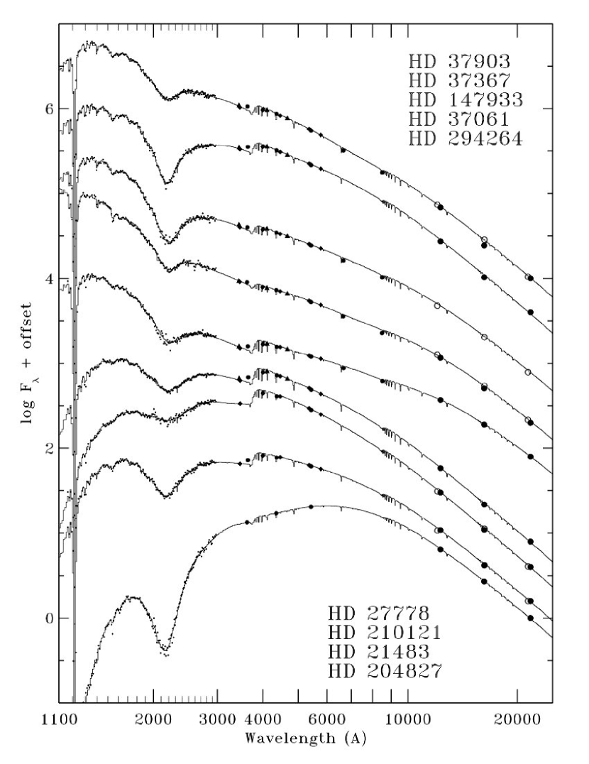
Figure 6: Same as Figure 3, but for a group of nine moderately reddened early B stars.

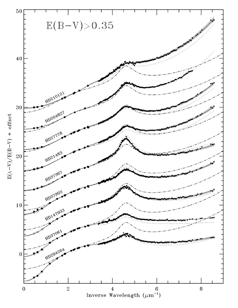
Figure 7: Same as Figure 4, but for nine moderately reddened early B stars. Dotted curves show pair method extinction curves for all stars except HD 294264. Those for HD 210121 and HD 27778 are unpublished results by us, and the rest are from the catalog of FM90. We are not aware of any pair method extinction curves for HD 294264. The values of $E(B-V)$ range from 0.36 to 1.08 for this group. These curves illustrate the wide range observed in the UV-through-IR wavelength dependence of interstellar extinction.

With our error estimates verified, we now examine how curves derived by the current approach compare to pair method curves. Figure 6 shows the UV-through-IR fits to the SEDs of a set of 9 moderately-reddened early-B stars, most of which are well known for their extinction properties, and Figure 7 shows the corresponding extinction curves. These stars were selected because they illustrate the wide range that exists in the wavelength dependence of both UV and IR extinction. For these stars the IR data allow us to determine the values of $R(V)$ and so the flexible extinction curve fits are shown throughout the IR-to-UV domain. As for the IC 4665 stars, all the parameters describing the fits are given in Tables 1 and 2.

Also shown in Figure 7 are UV curves based on the pair method technique. The curve for HD 294264 is from Valencic, Clayton, & Gordon (2004); the curves for HD 210121 and HD 27778 are from unpublished measurements by us; and the others are from the catalog of FM90. The agreement between the model-based and pair method curves is reasonable, and much better than seen for IC 4665. This is consistent with spectral mismatch as the prime cause of the existing discrepancies, since the nine stars have both higher $E(B-V)$ values and earlier spectral types than the IC 4665 stars, both of which tend to reduce the influence of mismatch errors. Note also that the best agreement between the pair method and the model-based curves occurs for the star HD 204827, for which identical results are found. Again, this is as it should be, since its $E(B-V)$ is the largest of any star in the sample, minimizing the impact mismatch effects. The 1-$\sigma$ uncertainties for our flexible extinction curve fits are indicated by shaded regions around the curves, as in Figure 4.

The curves shown in Figure 7 demonstrate the ability of the parameterized, flexible extinction curve (see §3.2) to conform itself to the wide range of extinction curve shapes encountered in interstellar space.

5.3 Lightly-Reddened Stars

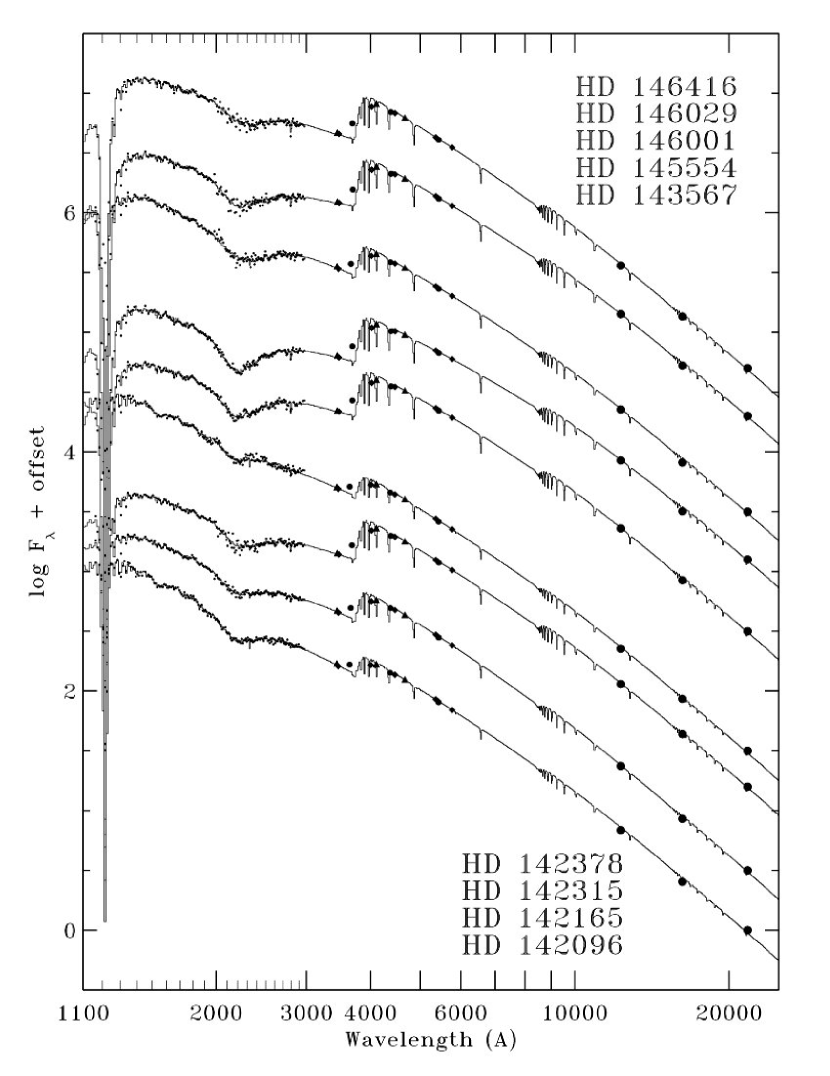
Figure 8: Same as Figure 3, but for a group of nine lightly-reddened mid-to-late B stars in the direction $347\arcdeg<l<355\arcdeg$ and $18\arcdeg<b<26\arcdeg$.

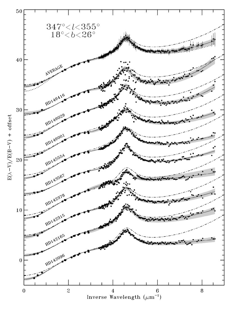
Figure 9: Same as Figure 4, but for a group of nine lightly-reddened mid-to-late B stars in the direction $347\arcdeg<l<355\arcdeg$ and $18\arcdeg<b<26\arcdeg$. The values of $E(B-V)$ range from 0.09 to 0.22 for this group. The dotted curve, superimposed on the average curve at the top of the figure shows the result for the nearby star HD 147933, located at ($l$, $b$) = ($353.7\arcdeg,17.7\arcdeg$) with $E(B-V)=0.50$ (see Figure 7).

Figure 8 shows a set of nine SED fits for low color excess stars (0.10 $\leq E(B-V)\leq$ 0.21) located along sightlines bounded by the Galactic coordinates $347\arcdeg<l<355\arcdeg$ and $18\arcdeg<b<26\arcdeg$. Figure 9 shows the corresponding extinction curves. These stars are all mid-to-late B members of the Upper Scorpius complex (Garrison 1967) and we encountered them while testing a procedure for scanning the IUE archives and automatically generating model-based extinction curves for stars in the appropriate spectral range. When examining the results for this pilot program which sampled high-latitude stars, it became obvious that curves derived from stars in this specific region demonstrated similar curve morphology which is distinctly different from the Galactic average. Given the low reddening and preponderance of late B stars, this strong systematic behavior would be missed by a pair method survey, with its large inherent mismatch errors.

Strong regional signatures are important in extinction studies because they may highlight the effects of specific physical processes on dust grain populations. Although we will examine this specific region in the future, two points are worth mentioning. First, it is important that similar curves result from stars with spectral types ranging from B2.5 to B9, verifying that the curves are not the result of some temperature-dependent systematic effect in fitting process. It is also worth noting that the region is near the $\rho$ Oph dark cloud. The star $\rho$ Oph A (HD 147933, whose extinction curve is shown in Figure 7) is located at a comparable distance and just south of the region, at Galactic coordinates of ($l$, $b$) = ($353.7\arcdeg,17.7\arcdeg$). The mean curve for the nine lightly-reddened stars is shown at the top of Figure 9, along with the average Galactic curve (dash-dot curve) and the HD 1479433 curve (dotted curve) for comparison. In the UV, the regional curve is seen to be almost identical to that for the more heavily-reddened HD 147933 ($E(B-V)\simeq 0.5$), suggesting that the sightlines sample similar dust populations. Interestingly, however, the curves are not identical in the IR. The mean 2MASS JHK data for the nine star sample implies a value of $R(V)\simeq 3.4$, slightly larger than the Galactic mean of 3.1, while HD 147933 has a value of $R(V)\simeq 4.3$. This contrast between UV and IR behavior may indicate different physical processes at work along the higher density sightline towards HD 147933, or perhaps different timescales in the response of UV and IR extinction to modifications of dust grain properties.

In producing the extinction curves for these lightly reddened stars, we found that, in some cases, the value of $k_{IR}$ was very poorly determined and produced (presumably) spurious “bumps and wiggles” in the IR portion of the curves. To eliminate this effect, we imposed a constraint on $k_{IR}$ for the whole sample, namely $k_{IR}=0.63R(V)-0.84$. This is taken from F04, who found a very strong relationship between $R(V)$ and $k_{IR}$ from a larger sample of more heavily reddened stars (see Figure 6 of F04). The ability to impose scientifically reasonable constraints on the fitting procedure is a major advantage of the extinction-without-standards approach, and can potentially allow high quality extinction results to be derived from stars with even lower reddenings than those shown in Figure 9.

6 DISCUSSION

In the previous sections we first provided an overview of the process used to determine an extinction curve, clarifying the measurement process. We then presented a new method for deriving UV-through-IR extinction curves, based on the use of stellar atmosphere models to provide estimates of the intrinsic (unreddened) stellar SEDs rather than unreddened (or lightly reddened) “standard” stars. We have shown that this “extinction-without-standards” technique greatly increases the accuracy of the derived extinction curves, particularly in the cases of low reddening and cool spectral types (i.e., late-B), and allows a realistic estimation of the uncertainties. A side benefit of the technique is the simultaneous determination of fundamental properties of the reddened stars themselves ($T_{\rm eff}$, $\log g$, [m/H], and $v_{turb}$), making the procedure valuable for both stellar and interstellar studies. Given the physical limitations of the ATLAS9 models we currently employ, the technique is limited to near main sequence B stars. However, in principal, the procedure can be adapted to any class of star for which accurate model SEDs are available and for which the signature of interstellar reddening can be distinguished from those of the stellar parameters. Although we developed the procedure based on IUE spectrophotometry in the UV, and photometry in the optical and near-IR (requiring a calibration of synthetic optical and near-IR photometry), the ideal application of the technique would be with spectrophotometric data throughout the UV-through-IR domain, allowing the most detailed examination of the wavelength dependence of the extinction curves.

The specific scientific advantages afforded by the extinction-without-standards technique can be summarized as follows:

Increased Precision: The increased precision in the derived extinction curves allows us to improve our understanding of extinction in a number of ways. First and most simply, we will determine the basic UV-to-IR wavelength dependence of extinction along a wide variety of sightlines more precisely than has been possible in the past. Second — and given that we know that extinction curve morphology varies widely from sightline-to-sightline (see Figure 7!) — we will be able to study the form of the variability and search for relationships between various features and wavelength domains using a data set with small and well-defined uncertainties. Such relationships, e.g., the correlation between $R(V)$ and the steepness of UV extinction discovered by Cardelli et al. (1989), provide important constraints on the dust grain population causing the extinction. Non-correlations can be equally important. For example, the lack of a correlation between the position and width of the 2175 Å bump demonstrated by Fitzpatrick & Massa (1986) remains a strong constraint on models for the bump carrier (Draine 2003). In either case, a precise knowledge of the measurement errors is required for transforming an observation into a scientific constraint. Finally, we will be able to place much stronger and more well-defined limits on the relationship between extinction curve morphology and interstellar environment. Curves derived from lines of sight to specific, localized regions, such as towards open clusters, can be particularly useful for relating curve properties to physical processes occurring in the interstellar medium (see, e.g., the study of Cepheus OB3 by Massa & Savage 1984 and Trumpler 37 by Clayton & Fitzpatrick 1987).

Access to lightly-reddened sightlines: The ability to accurately probe low $E(B-V)$ sightlines (as exemplified in Figures 4 and 9) opens the door to studies of dust in regions that have not been thoroughly explored. These include halo dust, dust in very low density regions, and local dust. Halo dust is especially important since we must contend with its effects every time we look out of the Galaxy. There are indications (Kiszkurno-Koziej & Lequeux 1987) that its properties differ systematically from dust at lower Galactic altitudes, and this result needs to be verified on a star-by-star basis. The nature of low density dust provides insights into the processing which occurs in hostile environments. Clayton et al. (2000) presented observations of dust from low density sightlines, and their results were intriguing. However, they were forced to select sightlines which accumulate fairly substantial color excesses, introducing the possibility of mixed grain populations. Furthermore, the results for their least-reddened sightlines were, as they acknowledge, poorly determined, forcing them to base their conclusions on a global average of properties of their sample. Finally, measuring the properties of local dust is important because it allows us to search for isolated, relatively homogeneous environments with uniform extinction curve shapes. These may signal physically and kinematically isolated regions which would be ideal for follow up interstellar line studies. In addition, Hipparcos parallax data exist for nearby stars and provide an opportunity to study the 3-dimensional structure of local extinction.

Access to the mid-to-late B stars: These stars are especially important because their space density is higher than that of the early-B stars usually used in extinction studies and thus their inclusion increases the number of stars available to create curves for nearby sightlines. Study of the mid-to-late B stars will enable the examination of the spatial structure of local dust absorption more thoroughly than previously possible and will greatly enhance our understanding of the local interstellar medium. The ability to construct accurate curves for mid-to-late B stars will also allow us to study extinction in open clusters and associations which are dominated by these stars, such as the Pleiades, $\alpha$ Per cluster, and IC 4665 (see Figure 4).

Automation: Because our model atmosphere approach does not require human intervention, once the basic data have been assembled, it is possible to process large data sets at one time. Naturally, the automated results must be inspected for outliers and data anomalies. Nevertheless, this approach reduces the work load considerably and a first-attempt yielded the regional anomaly shown in Figure 9. Furthermore, since the results are produced in a uniform manner, it is a relatively simple matter to inspect them for correlations between various curve properties, for anomalous curve shapes, and for spatial trends on the sky.

Stellar properties: In addition to dust parameters, our technique provides a meaningful, quantitative physical properties for the reddened stars. The temperature and surface gravity information will be useful for population studies of B stars in the field and in clusters. However, perhaps the most useful property will be the metallicity. We have demonstrated that several stars in the same cluster, which have a range in temperatures and gravities, all yield the same [m/H]. This verifies the sensitivity of our fitting procedure to this important quantity. As a result, we are confident that application of our procedure to large scale surveys of reddened, near main sequence B stars can provide a census of the distribution of metallicity throughout the Galaxy and the local universe.

Table 1: Best-Fit Parameters for Stars in Figures 3–9

Star	Spectral	$T_{eff}$	$\log g$	[m/H]	$v_{turb}$	$\theta_{R}$	$E(B-V)$
	Type	(K)			$\rm(km/s)$	(mas)	(mag)
FIGURES 3 & 4:
HD 161165	B8.5 V	$11774\pm 106$	$3.79\pm 0.10$	$-0.53\pm 0.06$	$0.4\pm 0.4$	$0.0320\pm 0.0004$	$0.19\pm 0.00$
HD 161184	B8 V	$11438\pm 108$	$4.05\pm 0.09$	$-0.54\pm 0.06$	$1.5\pm 0.3$	$0.0426\pm 0.0005$	$0.16\pm 0.00$
HD 161572	B6 V	$14968\pm 494$	$3.94\pm 0.13$	$-0.49\pm 0.07$	$0$	$0.0414\pm 0.0009$	$0.15\pm 0.01$
HD 161573	B3 IV	$16574\pm 511$	$3.93\pm 0.13$	$-0.40\pm 0.05$	$0$	$0.0563\pm 0.0010$	$0.20\pm 0.01$
HD 161603	B5 IV	$14734\pm 448$	$3.79\pm 0.12$	$-0.52\pm 0.06$	$0$	$0.0482\pm 0.0010$	$0.18\pm 0.01$
HD 161660	B7 V	$15468\pm 510$	$4.05\pm 0.12$	$-0.54\pm 0.09$	$2.2\pm 1.0$	$0.0374\pm 0.0007$	$0.16\pm 0.01$
HD 161677	B5 IV	$15194\pm 406$	$3.63\pm 0.13$	$-0.50\pm 0.05$	$0$	$0.0527\pm 0.0009$	$0.19\pm 0.01$
HD 161734	B8 V	$13125\pm 292$	$3.47\pm 0.12$	$-0.53\pm 0.06$	$0$	$0.0294\pm 0.0004$	$0.25\pm 0.01$
HD 162028	B6 V	$14056\pm 299$	$4.05\pm 0.10$	$-0.49\pm 0.06$	$0$	$0.0451\pm 0.0007$	$0.15\pm 0.01$
FIGURES 6 & 7:
HD 21483	B3 III	$19741\pm 979$	$3.55\pm 0.54$	$-0.25\pm 0.15$	$0$	$0.0710\pm 0.0018$	$0.56\pm 0.01$
HD 27778	B4 V	$17176\pm 492$	$4.05\pm 0.14$	$-0.33\pm 0.04$	$0$	$0.0815\pm 0.0018$	$0.37\pm 0.01$
HD 37061	B1 V	$30734\pm 452$	$4.3$	$-0.64\pm 0.04$	$8$	$0.0804\pm 0.0012$	$0.56\pm 0.00$
HD 37367	B2 IV-V	$19850\pm 603$	$3.56\pm 0.19$	$-0.29\pm 0.09$	$3.5\pm 1.2$	$0.0961\pm 0.0021$	$0.41\pm 0.01$
HD 37903	B1.5 V	$23677\pm 907$	$4.3$	$-0.28\pm 0.05$	$0$	$0.0389\pm 0.0010$	$0.37\pm 0.01$
HD 147933	B2 IV	$25032\pm 1098$	$4.3$	$-0.32\pm 0.07$	$0$	$0.2280\pm 0.0067$	$0.49\pm 0.01$
HD 204827	B0 V	$31063\pm 390$	$4.3$	$-0.65\pm 0.08$	$8$	$0.0508\pm 0.0011$	$1.09\pm 0.01$
HD 210121	B3 V	$18024\pm 1079$	$3.26\pm 0.47$	$-0.74\pm 0.09$	$0$	$0.0405\pm 0.0012$	$0.38\pm 0.01$
HD 294264	B3 Vn	$19830\pm 802$	$4.3$	$-0.54\pm 0.08$	$0$	$0.0412\pm 0.0010$	$0.52\pm 0.01$
FIGURES 8 & 9:
HD 142096	B2.5 V	$18039\pm 482$	$4.3$	$-0.11\pm 0.05$	$0$	$0.1250\pm 0.0021$	$0.17\pm 0.01$
HD 142165	B6 IVn	$14402\pm 287$	$4.3$	$-0.70\pm 0.06$	$0$	$0.1144\pm 0.0014$	$0.13\pm 0.01$
HD 142315	B8 Vnn	$12009\pm 108$	$4.24\pm 0.08$	$-0.76\pm 0.07$	$1.8\pm 0.4$	$0.0692\pm 0.0009$	$0.13\pm 0.00$
HD 142378	B3 V	$17434\pm 712$	$4.3$	$-0.21\pm 0.17$	$0.9\pm 2.6$	$0.0828\pm 0.0018$	$0.17\pm 0.01$
HD 143567	B9 Va	$11226\pm 43$	$4.3$	$-0.54\pm 0.04$	$0$	$0.0636\pm 0.0007$	$0.16\pm 0.00$
HD 145554	B9 Van	$11203\pm 75$	$4.29\pm 0.06$	$-0.71\pm 0.06$	$0$	$0.0600\pm 0.0009$	$0.21\pm 0.00$
HD 146001	B7 IV	$13922\pm 256$	$4.3$	$-0.68\pm 0.08$	$1.4\pm 0.6$	$0.0945\pm 0.0015$	$0.17\pm 0.01$
HD 146029	B9 Va	$10790\pm 68$	$4.11\pm 0.08$	$-0.84\pm 0.07$	$1.5\pm 0.4$	$0.0619\pm 0.0007$	$0.14\pm 0.00$
HD 146416	B9 Vnn	$11394\pm 82$	$4.13\pm 0.08$	$-0.53\pm 0.04$	$0$	$0.0756\pm 0.0009$	$0.10\pm 0.00$

Table 2: Best-Fit Extinction Curve Parameters for Stars in Figures 3–9

	IR Coefficients			Optical Spline Points				UV Coefficients
Star	$R(V)$	$k_{IR}$		$O_{1}$	$O_{2}$	$O_{3}$		$x_{0}$	$\gamma$	$c_{1}$	$c_{2}$	$c_{3}$	$c_{4}$
FIGURES 3 & 4:
HD 161165	$\cdots$	$\cdots$		$1.90\pm 0.11$	$1.32\pm 0.01$	$-0.00$		$4.54\pm 0.01$	$0.90\pm 0.05$	$0.58\pm 0.41$	$0.50\pm 0.08$	$2.80\pm 0.30$	$0.80\pm 0.05$
HD 161184	$\cdots$	$\cdots$		$1.87\pm 0.18$	$1.32\pm 0.02$	$-0.00$		$4.57\pm 0.01$	$0.84\pm 0.06$	$0.63\pm 0.44$	$0.47\pm 0.07$	$2.43\pm 0.28$	$0.93\pm 0.07$
HD 161572	$\cdots$	$\cdots$		$1.53\pm 0.35$	$1.27\pm 0.03$	$-0.01$		$4.59\pm 0.01$	$0.84\pm 0.04$	$0.69\pm 0.52$	$0.40\pm 0.10$	$3.09\pm 0.29$	$0.50\pm 0.07$
HD 161573	$\cdots$	$\cdots$		$1.65\pm 0.21$	$1.29\pm 0.02$	$-0.01$		$4.58\pm 0.01$	$0.86\pm 0.06$	$0.65\pm 0.40$	$0.36\pm 0.09$	$2.93\pm 0.33$	$0.41\pm 0.04$
HD 161603	$\cdots$	$\cdots$		$1.67\pm 0.27$	$1.29\pm 0.02$	$-0.01$		$4.57\pm 0.01$	$0.88\pm 0.04$	$0.77\pm 0.38$	$0.33\pm 0.08$	$3.31\pm 0.27$	$0.42\pm 0.04$
HD 161660	$\cdots$	$\cdots$		$1.30\pm 0.31$	$1.25\pm 0.03$	$-0.01$		$4.57\pm 0.01$	$1.09\pm 0.07$	$-0.74\pm 0.50$	$0.69\pm 0.09$	$4.78\pm 0.70$	$0.41\pm 0.05$
HD 161677	$\cdots$	$\cdots$		$1.78\pm 0.23$	$1.30\pm 0.02$	$-0.01$		$4.56\pm 0.01$	$0.95\pm 0.04$	$0.29\pm 0.42$	$0.48\pm 0.08$	$3.47\pm 0.31$	$0.41\pm 0.05$
HD 161734	$\cdots$	$\cdots$		$2.03\pm 0.18$	$1.33\pm 0.02$	$-0.00$		$4.57\pm 0.01$	$1.06\pm 0.03$	$0.12\pm 0.25$	$0.54\pm 0.05$	$4.28\pm 0.24$	$0.48\pm 0.03$
HD 162028	$\cdots$	$\cdots$		$1.81\pm 0.27$	$1.30\pm 0.02$	$-0.01$		$4.57\pm 0.01$	$0.85\pm 0.05$	$0.60\pm 0.47$	$0.43\pm 0.10$	$3.19\pm 0.29$	$0.55\pm 0.06$
FIGURES 6 & 7:
HD 21483	$2.90\pm 0.06$	$0.98\pm 0.09$		$2.25\pm 0.08$	$1.35\pm 0.01$	$0.00$		$4.62\pm 0.01$	$1.10\pm 0.04$	$-0.41\pm 0.24$	$0.89\pm 0.06$	$2.85\pm 0.23$	$0.57\pm 0.03$
HD 27778	$2.63\pm 0.09$	$0.79\pm 0.13$		$2.22\pm 0.10$	$1.34\pm 0.01$	$-0.00$		$4.61\pm 0.01$	$1.18\pm 0.03$	$-0.79\pm 0.19$	$0.94\pm 0.04$	$3.57\pm 0.19$	$0.72\pm 0.02$
HD 37061	$4.51\pm 0.06$	$2.11\pm 0.07$		$1.93\pm 0.03$	$1.33\pm 0.01$	$-0.00$		$4.58\pm 0.00$	$0.89\pm 0.02$	$1.74\pm 0.16$	$0.16\pm 0.02$	$1.34\pm 0.06$	$0.05\pm 0.01$
HD 37367	$2.98\pm 0.10$	$0.95\pm 0.15$		$2.08\pm 0.06$	$1.31\pm 0.01$	$0.00$		$4.60\pm 0.00$	$0.83\pm 0.01$	$1.37\pm 0.27$	$0.41\pm 0.05$	$2.98\pm 0.08$	$0.28\pm 0.03$
HD 37903	$3.85\pm 0.10$	$1.68\pm 0.13$		$2.01\pm 0.09$	$1.33\pm 0.01$	$-0.01$		$4.63\pm 0.00$	$0.97\pm 0.04$	$1.27\pm 0.24$	$0.35\pm 0.05$	$2.25\pm 0.16$	$0.49\pm 0.03$
HD 147933	$4.30\pm 0.08$	$1.92\pm 0.10$		$1.97\pm 0.07$	$1.32\pm 0.01$	$0.00$		$4.57\pm 0.00$	$0.97\pm 0.02$	$1.43\pm 0.20$	$0.23\pm 0.04$	$3.09\pm 0.12$	$0.33\pm 0.02$
HD 204827	$2.45\pm 0.05$	$0.75\pm 0.07$		$2.17\pm 0.03$	$1.37\pm 0.01$	$0.01$		$4.62\pm 0.00$	$0.99\pm 0.02$	$-1.55\pm 0.10$	$1.25\pm 0.02$	$2.68\pm 0.07$	$0.85\pm 0.03$
HD 210121	$2.19\pm 0.11$	$0.67\pm 0.14$		$2.76\pm 0.11$	$1.40\pm 0.01$	$-0.01$		$4.52\pm 0.01$	$1.35\pm 0.08$	$-3.05\pm 0.29$	$1.78\pm 0.08$	$3.41\pm 0.48$	$0.76\pm 0.02$
HD 294264	$5.55\pm 0.08$	$2.87\pm 0.10$		$1.85\pm 0.08$	$1.31\pm 0.01$	$0.01$		$4.57\pm 0.01$	$1.02\pm 0.04$	$1.62\pm 0.14$	$0.08\pm 0.04$	$2.07\pm 0.15$	$0.24\pm 0.01$
FIGURES 8 & 9:
HD 142096	$3.82\pm 0.24$	$1.56\pm 0.15$		$2.02\pm 0.17$	$1.31\pm 0.02$	$-0.00$		$4.59\pm 0.01$	$0.87\pm 0.03$	$1.23\pm 0.27$	$0.29\pm 0.07$	$2.47\pm 0.16$	$0.07\pm 0.03$
HD 142165	$3.08\pm 0.26$	$1.10\pm 0.16$		$1.87\pm 0.30$	$1.30\pm 0.03$	$-0.01$		$4.61\pm 0.01$	$0.85\pm 0.04$	$0.73\pm 0.40$	$0.49\pm 0.07$	$2.63\pm 0.22$	$0.23\pm 0.05$
HD 142315	$3.37\pm 0.34$	$1.28\pm 0.21$		$1.96\pm 0.18$	$1.32\pm 0.02$	$-0.00$		$4.57\pm 0.02$	$0.85\pm 0.07$	$0.98\pm 0.50$	$0.38\pm 0.09$	$2.66\pm 0.40$	$0.29\pm 0.07$
HD 142378	$3.64\pm 0.18$	$1.45\pm 0.11$		$2.28\pm 0.25$	$1.33\pm 0.02$	$-0.00$		$4.64\pm 0.02$	$0.63\pm 0.08$	$1.51\pm 0.40$	$0.41\pm 0.08$	$0.91\pm 0.22$	$0.09\pm 0.06$
HD 143567	$2.76\pm 0.18$	$0.90\pm 0.12$		$1.88\pm 0.08$	$1.33\pm 0.01$	$-0.00$		$4.59\pm 0.01$	$0.92\pm 0.06$	$0.12\pm 0.52$	$0.51\pm 0.09$	$3.53\pm 0.45$	$0.24\pm 0.08$
HD 145554	$3.65\pm 0.19$	$1.46\pm 0.12$		$1.79\pm 0.10$	$1.31\pm 0.01$	$0.00$		$4.58\pm 0.01$	$0.95\pm 0.05$	$0.76\pm 0.40$	$0.33\pm 0.07$	$3.54\pm 0.34$	$0.24\pm 0.06$
HD 146001	$3.53\pm 0.22$	$1.38\pm 0.14$		$1.69\pm 0.22$	$1.29\pm 0.02$	$-0.00$		$4.54\pm 0.01$	$1.26\pm 0.15$	$0.12\pm 0.74$	$0.43\pm 0.11$	$6.00\pm 1.61$	$0.30\pm 0.05$
HD 146029	$3.56\pm 0.27$	$1.40\pm 0.17$		$2.11\pm 0.17$	$1.34\pm 0.01$	$-0.00$		$4.57\pm 0.02$	$0.88\pm 0.07$	$1.85\pm 0.57$	$0.18\pm 0.11$	$3.30\pm 0.46$	$0.62\pm 0.11$
HD 146416	$2.81\pm 0.36$	$0.93\pm 0.23$		$2.05\pm 0.22$	$1.34\pm 0.02$	$-0.01$		$4.53\pm 0.02$	$0.89\pm 0.08$	$0.45\pm 0.82$	$0.44\pm 0.16$	$3.08\pm 0.57$	$0.76\pm 0.15$

Table 3: Mean Extinction Parameters for IC 4665

Parameter	Weighted	Sample	RMS of	Implied
	Mean	Standard Deviation	Monte Carlo Errors	Intrinsic Scatter
$O_{1}$	$1.819$	$0.219$	$0.244$	$\cdots$
$O_{2}$	$1.306$	$0.024$	$0.021$	$0.012$
$O_{3}$	$-0.004$	$0.003$	$0.001$	$0.003$
$x_{0}$	$4.569$	$0.015$	$0.011$	$0.010$
$\gamma$	$0.922$	$0.096$	$0.050$	$0.081$
$c_{1}$	$0.380$	$0.475$	$0.428$	$0.206$
$c_{2}$	$0.478$	$0.108$	$0.085$	$0.067$
$c_{3}$	$3.273$	$0.736$	$0.359$	$0.643$
$c_{4}$	$0.500$	$0.191$	$0.052$	$0.184$
$A_{bump}$	$5.633$	$0.709$	$0.319$	$0.634$

Figure 1: Effects of a $\pm\frac{1}{2}$-class spectral mismatch error on extinction curves derived by the pair method. In each of the four groups, the solid curve shows the true shape of a normalized (but arbitrarily offset) extinction curve affecting a B1, B2, B5, or B9 star. The dashed and dash-dot curves show the extinction curves which would be derived via the pair method in the presence of a $\pm\frac{1}{2}$ spectral type mismatch error in the cases of $E(B-V)=0.30$ and $E(B-V)=0.15$, respectively. Detailed spectrophotometric extinction curves are typically only available in the UV spectral region, which is highlighted in the figure. The extension of the mismatch curves into the optical and IR is shown by the dotted curves. Note that the mismatch curves fall below the true curve in the UV and above the true curve in the IR when the standard star is cooler than the reddened star, and vice versa. The feature in the mismatch curves near $1/\lambda\simeq 2.7\mu{\rm m}^{-1}$ is due to the Balmer jump. The large feature at 8.2 $\mu{\rm m}^{-1}$ (i.e., 1215 Å) is due to mismatch of the strong stellar Lyman $\alpha$ absorption line. In producing these curves, we use the temperature scale: B0.5 = 28000 K, B1 = 25000 K, B2 = 20000 K, B3 = 18000 K, B5 = 15000 K, B7 = 13000 K, B8 = 12000 K, B9 = 11000 K, and A0 = 9500 K.

Figure 2: A flexible, parametrized representation of the IR through UV extinction curve. The curve consists of two parts: 1) the UV (i.e., $\lambda\leq 2700$ Å, solid curve in the figure) where we adopt the 3-component parametrization scheme of FM90; and 2) the optical/IR (i.e., $\lambda>2700$ Å, dashed curve) where we adopt a cubic spline interpolation through sets of IR ($I_{1}$,$I_{2}$, $I_{3}$, $I_{4}$), optical ($O_{1}$, $O_{2}$, $O_{3}$, $O_{4}$), and UV ($U_{1}$, $U_{2}$) “anchor points.” The values of the anchor points and the six parameters describing the UV portion of the curve are determined by fitting the observed SED of a reddened star, as described in §3. The dotted line shows the “linear component” of the UV extinction curve. The other two components, which are added to the linear component, are the 2175 Å bump profile centered at $\lambda^{-1}\simeq 4.6\mu{\rm m}^{-1}$ and the far-UV rise, which refers to the departure of the curve from the extrapolation of the linear component at very short wavelengths. See the discussion in §3.2. The particular curve shown in this figure corresponds to that derived in §5.2 for the star HD 147933.

References

- Asplund et al. (2005) Asplund, M. Grevesse, N., & Sauval, A.J. 2005, in ASP Conf. Ser. 336, Cosmic Abundances as Records of Stellar Evolution and Nucleosynthesis, eds. T.G. Barnes & F.N. Bash (San Francisco: ASP), in press
- Bohlin (1996) Bohlin, R. C. 1996, AJ, 111, 1743
- Bohlin, Savage, & Drake (1978) Bohlin, R.C., Savage, B.D., Drake, J.F. 1978, ApJ, 224, 132.
- Cardelli et al. (1989) Cardelli, J.A., Clayton, G.C. & Mathis, J.S. 1989, ApJ, 345, 245
- Cardelli et al. (1992) Cardelli, J.A., Sembach, K., & Mathis, J.S. 1992, AJ, 104, 1916.
- Clayton & Fitzpatrick (1987) Clayton, G.C., & Fitzpatrick, E.L. 1987, AJ, 93, 157
- Clayton et al. (2000) Clayton, G.C., Gordon, K.D., & Wolff, M.J. 2000, ApJS, 129, 147
- (8) Diplas, A. & Savage, B.D. 1994, ApJS, 93, 211
- Draine (2003) Draine, B.T. 2003, ARA&A, 41, 241
- Fitzpatrick (1999) Fitzpatrick, E.L. 1999, PASP, 111, 63
- Fitzpatrick et al. (2003) Fitzpatrick, E.L., Ribas, I., Guinan, E.F., Maloney, F.P., & Claret, A. 2003, ApJ, 587, 685
- Fitzpatrick (2004) Fitzpatrick, E.L. 2004, in Astrophysics of Dust, eds. A.N. Witt, G.C. Clayton, & B.T. Draine, ASP Conference Series, Vol. 309, 33 (F04)
- Fitzpatrick & Massa (1986) Fitzpatrick, E.L., & Massa D. 1986, ApJ, 307, 286
- Fitzpatrick & Massa (1988) Fitzpatrick, E.L., & Massa D. 1988, ApJ, 328, 734
- Fitzpatrick & Massa (1990) Fitzpatrick, E.L., & Massa D. 1990, ApJS, 72, 163 (FM90)
- Fitzpatrick & Massa (1999) Fitzpatrick, E.L., & Massa D. 1999, ApJ, 525, 1011 (FM99)
- Fitzpatrick & Massa (2005) Fitzpatrick, E.L., & Massa D. 2005, AJ, in press (FM05)
- Garrison (1967) Garrison, R.F. 1967, ApJ, 147, 1003
- Hackwell et al. (1991) Hackwell, J.A., Hecht, J.H., & Tapia, M. 1991, ApJ, 375, 163 (HHT)
- Kiszkurno-Koziej & Lequeux (1987) Kiszkurno-Koziej, E., & Lequeux, J. 1987, A&A, 185, 291
- Kurucz (1991) Kurucz, R. L. 1991, in Stellar Atmospheres: Beyond Classical Models, ed. L. Crivellari, I. Hubeny, & D. G. Hummer (NATO ASI Ser. C.; Dordrect: Reidel), 441
- Martin & Whittet (1990) Martin, P.G., & Whittet, D.C.B. 1990, ApJ, 357, 113
- Massa & Fitzpatrick (1986) Massa, D., Fitzpatrick, E.L. 1986, ApJS, 60, 305
- Massa & Fitzpatrick (2000) Massa, D., & Fitzpatrick, E.L. 2000, ApJS, 126, 517 (MF00)
- Massa & Savage (1984) Massa, D., & Savage, B.D. 1984, ApJ, 279, 310
- Massa et al. (1983) Massa, D., Savage, B.D., & Fitzpatrick, E.L. 1983, ApJ, 266, 662
- Mermilliod et al., (1997) Mermilliod, J.-C., Mermilliod, M., & Hauck, B. 1997 A&AS, 124, 349
- Nichols & Linsky, (1996) Nichols, J.S. & Linsky, J.L. 1996, AJ, 111, 517
- Reike & Lebofsky (1985) Rieke, G.H., & Lebofsky, M.J. 1985, ApJ, 288, 618
- Whiteoak, (1966) Whiteoak, J. B. 1966, ApJ, 144, 305
- Valencic et al. (2004) Valencic, L.A., Clayton, G.C., & Gordon, K.D. 2004, ApJ, 616, 912