Compact Stars for Undergraduates

Abstract

We report on an undergraduate student project initiated in the summer semester of 2004 with the aim to establish equations of state for white dwarfs and neutron stars for computing mass–radius relations as well as corresponding maximum masses. First, white dwarfs are described by a Fermi gas model of degenerate electrons and neutrons and effects from general relativity are examined. For neutron star matter, the influence of a finite fraction of protons and electrons and of strong nucleon–nucleon interactions are studied. The nucleon–nucleon interactions are introduced within a Hartree–Fock scheme using a Skyrme–type interaction. Finally, masses and radii of neutron stars are computed for given central pressure.

I Introduction

Compact stars, i.e. white dwarfs and neutron stars, are the final stages in the evolution of ordinary stars. After hydrogen and helium burning, the helium reservoir in the star’s core is burned up to carbon and oxygen. The nuclear processes in the core will stop and the star’s temperature will decrease. Consequently, the star shrinks and the pressure in the core increases.

As long as the star’s mass is above a certain value, it will be able to initialise new fusion processes to heavier elements. The smaller the mass, the more the core has to be contracted to produce the required heat for the next burning process to start. If the star’s initial mass is below eight solar masses, the gravitational pressure is too weak to reach the required density and temperature to initialise carbon fusion. Due to the high core temperature, the outer regions of the star swell and are blown away by stellar winds. What remains is a compact core mainly composed of carbon and oxygen. The interior consists of a degenerate electron gas which, as we will discuss, is responsible for the intrinsic high pressure. The compact remnant starts to emit his thermal energy and a white dwarf is born.

As there are no fusion processes taking place in the interior of the white dwarf, a different force than thermal pressure is needed to keep the star in hydrostatic equilibrium. Due to the Pauli principle, two fermions cannot occupy the same quantum state, hence, more than two electrons (with different spin) cannot occupy the same phase space. With increasing density, the electrons fill up the phase space from the lowest energy state, i.e. the smallest momentum. Consequently, the remaining electrons sit in physical states with increasing momentum. The resulting large velocity leads to an adequate pressure of the electrons — the degeneracy pressure — counterbalancing gravity’s pull and stabilising the white dwarf.

The electrons are the first particles to become degenerate in dense matter due to their small mass. White dwarfs consist also of carbon and oxygen, but the contribution of nuclei to the pressure is negligible for the density region of interest here. The gravitational force increases with mass. Consequently, a larger degeneracy pressure, i.e. a greater density, is needed for stability for more massive white dwarfs. There is a mass limit for white dwarfs beyond which even the degenerate electron gas cannot prevent the star from collapsing. This mass limit is around 1.4 solar masses — the famous Chandrasekhar mass. For greater masses, the white dwarf collapses to a neutron star or a black hole. The radii of white dwarfs are in the range of 10,000 km — about the size of our planet earth.

Similarly, a neutron star is stabilised by the degeneracy pressure also. The difference is that for neutron stars the degeneracy pressure originates mainly from neutrons, not from electrons.

If the initial mass of an ordinary star exceeds eight solar masses, carbon and oxygen burning starts in the core. Around the core is a layer of helium and a layer of hydrogen, both taking part in fusion processes. As long as they produce the required temperature to keep the star in hydrostatic equilibrium, new burning processes to heavier elements will take place in the core while the fusion of lighter elements will continue in the outer shells. Once iron is produced in the core, there is no burning process left to generate energy as the fusion to heavier elements requires energy to be put in. So the mass of the iron core increase while its radius decrease as there is less thermal pressure to work against gravity. At some critical mass, the iron core collapses. The density increases so much that the electrons are captured by nuclei and combine with protons to form neutrons. Therefore, the atomic nuclei become more and more neutron–rich with increasing density. At some critical density, the nuclei are not able to bind all the neutrons any more, neutrons start to drop out and form a neutron liquid which surrounds the atomic nuclei. For even larger density there will be just a dense and incompressible core of neutrons with a small fraction of electrons and protons. Neutrons in neutron stars are then degenerate like electrons in white dwarfs.

There will be an outgoing shock wave generated by the proto–neutron star due to the high incompressibility of neutron star matter. The falling outer layers of the ordinary star bounce and move outwards interacting with the other still collapsing layers and generate an overall outward expansion — a core–collapse supernova arises. The neutron rich remnant of the core collapse will become a neutron star as long as his mass is less than about two to three solar masses, otherwise it proceeds to shrink and becomes finally a black hole. The radii of neutron stars are typically 10 km — the size of the city of Frankfurt.

During the summer semester of 2004, the two last coauthors organised a student project about compact stars on which we will give an extended report in the following. We derive the equations of state (EoS) for white dwarfs and neutron stars, respectively, where we will cover the Newtonian and the relativistic cases for both kinds of compact stars. These EoSs are used to determine numerically the masses and radii for a given central pressure. In the first chapter we give a short description of the properties of white dwarfs and neutron stars. We then proceed in the second chapter with calculations of the EoS for white dwarfs. We assume a Fermi gas model of degenerate electrons and outline two different ways which we employed for deriving the equations of state, repeat the basic structure equations for stars as well as the corrections from general relativity (the so called Tolman–Oppenheimer–Volkoff (TOV) equation) and discuss the Chandrasekhar mass, which is the famous mass limit for white dwarfs. From the third chapter on we will concentrate on neutron stars. Again we will have two different approaches for calculating the equation of state for neutron stars. After describing a pure neutron star, we will discuss the effect of the presence of protons and electrons which will appear in $\beta$–equilibrium. Furthermore, we will introduce a simple effective model for incorporating the nucleon–nucleon interactions. We will compare our results to the recent work by Reddy and Silbar Silbar and Reddy (2004) who are using different numerical methods and another model for the nucleon–nucleon interactions. We investigate whether the two model descriptions satisfy causality. Finally, we summarise our findings and give a short outline of modern developments in neutron star physics.

II White Dwarfs

II.1 Definitions

II.1.1 Structure equations

There are two forces acting on the star, one of them is gravitation and the second one arises from the pressure (thermal pressure for normal stars and degeneracy pressure for white dwarfs and neutron stars). The pressure and force are related in the standard way:

$${dp} = \frac{dF}{A}=\frac{dF}{4\pi r^{2}}\quad,$$ (1)

where $p$ denotes the pressure, $F$ the force, and $A$ is the area where the force takes effect. For the gravitational force one has for a spherical symmetric system:

$${dF} = -\frac{G{dm}\cdot m(r)}{r^{2}}\quad,$$ (2)

with $r$ being the radial distance of a spherical star and

$${dm} = \rho(r){dV}=\rho(r)4\pi r^{2}{dr}\quad.$$ (3)

Equating both expressions gives the first basic structure equation for stars in general:

$$\frac{dp}{dr} = -\frac{G\rho(r){m(r)}}{r^{2}}\quad.$$ (4)

Here $G$ is Newton’s Gravitational constant, $\rho$ is the mass density, $m$ is the mass up to radius r and $V$ is the volume. Again using eq. (3), one has also the equation:

$$\frac{dm}{dr} = \rho(r)4\pi r^{2}\quad.$$ (5)

We can rewrite the mass density in terms of the energy density $\epsilon$:

$$\rho(r) = \frac{\epsilon(r)}{c^{2}}\quad,$$ (6)

where $c$ is the speed of light. With these definitions one obtains structure equations which describe how the mass and the pressure of a star change with radius:

$$\frac{dm}{dr} = \frac{4\pi r^{2}\epsilon(r)}{c^{2}}$$ (7)

$$\frac{dp}{dr} = -\frac{G\epsilon(r)m(r)}{c^{2}r^{2}}\quad.$$ (8)

Here one has to solve two coupled differential equations. Note that while ${dm}/{dr}$ is positive, ${dp}/{dr}$ must always be negative. Starting with certain positive values for $m$ and $p$ in a small central region of the star the mass will increase while the pressure decreases eventually reaching zero. One sets $m(r=0)=0$ and, in addition, one has to specify some ”initial” central pressure ${p(r=0)=p_{0}}$ in order to solve for eqs. (7) and (8). The behaviour of $m$ and $p$ as a function of the radius will become important for our numerical computations.

II.1.2 Equations of state

From the last section, we arrived at two coupled differential equations for the mass and the pressure in a star where both depend on the energy density $\epsilon$. One needs to fix now the relation ${p(\epsilon)}$ between the pressure and the energy density in addition. Matter in white dwarfs can be treated as an ideal Fermi gas of degenerate electrons. For electrically neutral matter an adequate amount of protons to the electron gas has to be added. Furthermore, the protons combine with neutrons and form nuclei which will be also taken into account.

The distribution of fermions as an ideal gas in equilibrium in dependence of their energy is described by the Fermi–Dirac–Statistic:

$${f(E)} = \frac{1}{exp[(E-\mu)/k_{B}T]+1}\quad,$$ (9)

where $E$ is the energy, $\mu$ is the chemical potential, $k_{B}$ is the Boltzmann constant and $T$ is the temperature. In kinetic theory we find the following correlation between the distribution function ${f}$ and the number density $n_{i}=dN_{i}/dV$ in phase space for a certain particle species $i$:

$$\frac{dn_{i}}{d^{3}k} = \frac{g}{(2\pi\hbar)^{3}}f\quad,$$ (10)

$(2\pi\hbar)^{3}$ is the ”unit” volume of a cell in phase space and $g$ is the number of states of a particle with a given value of momentum $k$. For electrons $g$ equals 2. The number density of species $i$ is given by:

$${n_{i}} = \int dn_{i}=\int\frac{g}{(2\pi\hbar)^{3}}fd^{3}k\quad.$$ (11)

For degenerate fermions the temperature can be set to zero (as $(\mu-m_{e}c^{2})\gg k_{B}T$), accordingly $\mu/k_{B}T$ goes to infinity. To be added to the system, a particle must have an energy equal to the Fermi energy of the system as all the other energy levels are already filled. This description matches exactly the definition of the chemical potential, and so we can set here $\mu$= ${E_{F}}$. With all these assumptions we can write the distribution function as:

$$f(E) = \left\{\begin{array}[]{ccccc}1\quad\mbox{ for }\quad E\leq E_{F}\\ 0\quad\mbox{ for }\quad E>E_{F}\end{array}\right\}\quad.$$ (14)

If we ignore all electrostatic interactions, we can write for the number density of the degenerate electron gas:

$${n_{e}} = \int_{0}^{k_{F}}\frac{2}{(2\pi\hbar)^{3}}{d^{3}k}=\frac{8\pi}{(2\pi\hbar)^{3}}\int_{0}^{k_{F}}k^{2}dk=\frac{k_{F}^{3}}{3\pi^{2}\hbar^{3}}\quad.$$ (15)

As the star should be electrically neutral, each electron is neutralised by a proton. If we assume that the white dwarf is predominantly made of ${}^{12}{\rm C}$ or ${}^{16}{\rm O}$, $A/Z=2$. The proton and neutrons masses are both much larger than the electron’s one, so when we calculate the mass density in the white dwarf we can neglect the mass of the electrons and just concentrate on the nucleon mass $m_{N}$. The mass density in terms of $m_{N}$ is:

$$\rho=n\cdot{m_{N}}\cdot\frac{A}{Z}\quad,$$ (16)

where $n=n_{e}$. With this equation and the dependence of number density on $k_{F}$ we find:

$${k_{F}}=\hbar\left(\frac{3\pi^{2}\rho}{m_{N}}\frac{Z}{A}\right)^{1/3}\quad.$$ (17)

As the momentum of the nucleons is negligible compared to their rest mass, the nucleons do not give a significant contribution to the pressure at zero temperature. On the other hand, the electrons behave as a degenerate gas, and have large velocities which give the dominant contribution to the pressure. The energy density can be divided in two components, one term coming from nucleons and the other one coming from electrons, whereas the contribution from nucleons is dominating. The complete energy density can be written as Shapiro and Teukolsky (1983):

$$\epsilon = nm_{N}\frac{A}{Z}c^{2}+\epsilon_{\rm elec}(k_{F})\quad.$$ (18)

where $\epsilon_{\rm elec}(k_{F})$ is the energy density of electrons. With the electron energy

$$E(k) = \sqrt{{k^{2}}c^{2}+{m_{e}^{2}}c^{4}}$$ (19)

we can write $\epsilon_{elec}$ in the following way:

$$\epsilon_{\rm elec}(k_{F}) = \frac{8\pi}{(2\pi\hbar)^{3}}\int_{0}^{k_{F}}E(k)k^{2}dk$$ (20)

$$= \frac{8\pi}{(2\pi\hbar)^{3}}\int_{0}^{k_{F}}(k^{2}c^{2}+m_{e}^{2}c^{4})^{1/2}k^{2}dk$$

$$= \epsilon_{0}\int_{0}^{k_{F}/m_{e}c}(u^{2}+1)^{1/2}u^{2}du$$

$$= \frac{\epsilon_{0}}{8}\left[(2x^{3}+x)(1+x^{2})^{1/2}-\sinh^{-1}(x)\right]\$$

with

$$\epsilon_{0}=\frac{m_{e}^{4}c^{5}}{\pi^{2}\hbar^{3}}$$ (21)

and

$$x=k_{F}/m_{e}c.$$ (22)

The factor $\epsilon_{0}$ carries the dimension of an energy density (${\rm dyne/{cm^{2}}}$). The pressure of a system with an isotropic distribution of momenta is given by:

$$p = \frac{1}{3}\frac{8\pi}{(2\pi\hbar)^{3}}\int_{0}^{k_{F}}kvk^{2}dk$$ (23)

where the velocity $v={kc^{2}}/{E}$ and the factor ${1}/{3}$ comes from isotropy. For the electrons we get:

$$p(k_{F}) = \frac{1}{3}\frac{8\pi}{(2\pi\hbar)^{3}}\int_{0}^{k_{F}}\frac{k^{2}c^{2}}{E(k)}k^{2}dk$$ (24)

$$= \frac{8\pi}{3(2\pi\hbar)^{3}}\int_{0}^{k_{F}}(k^{2}c^{2}+m_{e}^{2}c^{4})^{-1/2}c^{2}k^{4}dk$$

$$= \frac{\epsilon_{0}}{3}\int_{0}^{k_{F}/m_{e}c}(u^{2}+1)^{-1/2}u^{4}du$$

$$= \frac{\epsilon_{0}}{24}\left[(2x^{3}-3x)(1+x^{2})^{1/2}+3\sinh^{-1}(x)\right].\$$

The energy density is dominated by the mass density of nucleons while the electrons contribute to most of the pressure.

We want to arrive at an equation of the form $p=p(\epsilon)$. In the following, let us consider the two extreme cases: $x\ll 1$ and $x\gg 1$, i.e. $k_{F}\ll m_{e}c$ and $k_{F}\gg m_{e}c$, respectively. In the former case, the kinetic energy is much smaller than the rest mass of the electrons, i.e. that is the non–relativistic case. Considering the equation for the pressure for $k_{F}\ll m_{e}c$ one finds that

$$p(k_{F})=\frac{\epsilon_{0}}{3}\int_{0}^{k_{F}/m_{e}c}(u^{2}+1)^{-1/2}u^{4}du\approx\frac{\epsilon_{0}}{3}\int_{0}^{k_{F}/m_{e}c}u^{4}du=\frac{\epsilon_{0}}{15}\left(\frac{k_{F}}{m_{e}c}\right)^{5}=\frac{\hbar^{2}}{15\pi^{2}m_{e}}\left(\frac{3\pi^{2}\rho Z}{m_{N}A}\right)^{5/3}\quad.$$ (25)

With the assumption $\epsilon=\rho\cdot c^{2}$ one arrives at the following equation of state (EoS) in the non–relativistic limit:

$$p \approx K_{\rm non-rel}\epsilon^{5/3}$$ (26)

with

$$K_{\rm non-rel} = \frac{\hbar^{2}}{15\pi^{2}m_{e}}\left(\frac{3\pi^{2}Z}{m_{N}c^{2}A}\right)^{5/3}\quad.$$ (27)

For the relativistic case ($k_{F}\gg m_{e}$) we arrive at:

$$p(\epsilon) \approx K_{\rm rel}\,\epsilon^{4/3}\quad,$$ (28)

where

$$K_{\rm rel}=\frac{\hbar c}{12\pi^{2}}\left(\frac{3\pi^{2}Z}{m_{N}c^{2}A}\right)^{4/3}\quad.$$ (29)

The relation of the form

$$p=K\epsilon^{\gamma}$$ (30)

is called a ”polytropic” equation of state. With the two EoSs for the relativistic and for the non–relativistic case we are in the position to calculate the mass and the radius of a white dwarf with a given central energy density by inserting these relations into the structure equations (7) and (8). A discussion on general forms of polytropic EoSs can be found in Herrera and Barreto (2004).

Besides the non–relativistic and the relativistic polytropic EoS there exists also a third case, which becomes important for later considerations — the ultra–relativistic EoS. Here one assumes for simplicity a relativistic pure electron Fermi gas with the total energy density:

$$\epsilon=\epsilon_{elec}(k_{F}).$$ (31)

Just like in eq. (20) one can calculate the energy density using

$$\epsilon(k_{F})=\epsilon_{0}\int_{0}^{k_{F}/m_{e}c}(u^{2}+1)^{1/2}u^{2}du,$$ (32)

getting for the relativistic case

$$\epsilon=\frac{\epsilon_{0}}{4}x^{4}\quad.$$ (33)

From eq. (24)

$$p(k_{F})=\frac{\epsilon_{0}}{3}\int_{0}^{k_{F}/m_{e}c}(u^{2}+1)^{-1/2}u^{4}du$$ (34)

one finds for $k_{F}\gg m_{e}$:

$$p=\frac{\epsilon_{0}}{12}x^{4}.$$ (35)

Therefore, one arrives at the general solution for an ultra–relativistic gas:

$$p=\frac{1}{3}\epsilon\quad.$$ (36)

This relation is also very important for neutron stars as a limiting case of their relativistic EoS.

II.1.3 Chandrasekhar mass

We will derive in this section the maximum mass for white dwarfs for a polytropic EoS as found by Chandrasekhar in 1931 Chandrasekhar (1931), following Weinberg (1972); Shapiro and Teukolsky (1983). Note, that already in 1932 Landau found with simple arguments a mass limit for white dwarfs and neutron stars Landau (1932) (see also the discussion in e.g. Shapiro and Teukolsky (1983)).

By straight–forward algebra the structure equations (7) and (8) can be combined to give:

$$\frac{1}{r^{2}}\frac{d}{dr}\left(\frac{r^{2}}{\rho}\frac{dp}{dr}\right) = -4\pi G\rho\quad.$$ (37)

The parameter $\gamma$ in the polytropic equation is usually rewritten as $\gamma=1+\frac{1}{n}$ where $n$ is the polytropic index.

Given the equation of state $p=p(\rho)$ in the polytropic form (see eq. (30))

$$p=K\epsilon^{\gamma}=K\rho^{\gamma}c^{2\gamma}$$ (38)

one can obtain $\rho(r)$ by solving eq. (37) with the initial conditions:

$$\rho(r=0)=\rho_{0}\neq 0$$ (39)

and

$$\left.\frac{d\rho}{dr}\right|_{(r=0)}=0$$ (40)

which follows from the condition ${m(r=0)=0}$ and eq. (8). Equation (37) can be transformed into a dimensionless form with the following substitutions:

$$r=a\xi\quad\mbox{\rm with }\quad a\equiv\left(\frac{(n+1)K\rho_{0}^{(1-n)/n}}{4\pi G}\right)^{1/2}c^{(n+1)/n}$$ (41)

and

$$\rho(r)=\rho_{0}\theta^{n}\quad\mbox{\rm with }\quad\theta=\theta(r)\quad.$$ (42)

Here $\theta$ and $\xi$ correspond to a dimensionless density and radius, respectively, and $a$ is a constant scale factor. With these definitions eq. (37) translates to:

$$\frac{1}{\xi^{2}}\frac{d}{d\xi}\left(\xi^{2}\frac{d\theta}{d\xi}\right) = -\theta^{n}.$$ (43)

Equation (43) is called the Lane–Emden equation for a given polytropic index $n$. From eq. (42) one realizes that

$$\theta(r=0)=1.$$ (44)

Furthermore, with eq. (40) the density distribution at the center of the star obeys:

$$\left.\frac{d\theta}{dr}\right|_{(r=0)}=0.$$ (45)

With the boundary conditions, eqs. (45) and (44), one can integrate eq. (43) numerically. One finds for $n<5$ and $\gamma>6/5$, respectively, that the solutions decrease monotonically with radius and have a zero for a $\xi=\xi_{1}$, i.e. $\theta(\xi_{1})=0$ or $\rho(r_{1}=a\xi_{1})=0$, respectively. Hence, the radius of the star is given by R $=r_{1}=a\xi_{1}$ which translates to

$$R = \left(\frac{(n+1)K\rho_{0}^{(1-n)/n}}{4\pi G}\right)^{1/2}c^{(n+1)/n}\xi_{1}.$$ (46)

Using eqs. (42) and (41) the total mass $M$ of the star can be calculated as follows:

$$M = \int_{0}^{R}4\pi r^{2}\rho dr$$ (47)

$$= 4\pi a^{3}\rho_{0}\int_{0}^{\xi_{1}}\xi^{2}\theta^{n}d\xi$$

$$= 4\pi c^{(3n+3)/n}\left(\frac{(n+1)K}{4\pi G}\right)^{3/2}\rho_{0}^{(3-n)/2n}\xi_{1}^{2}|\theta^{\prime}(\xi_{1})|.$$

For $\rho_{0}$ we can use eq. (46) and get:

$$M = 4\pi c^{(2n+2)/(n-1)}\left(\frac{(n+1)K}{4\pi G}\right)^{n/(n-1)}\xi_{1}^{(n-3)/(1-n)}\xi_{1}^{2}|\theta^{\prime}(\xi_{1})|R^{(3-n)/(1-n)}\quad.$$ (48)

The interesting case is the high density limit, i.e. the relativistic case with $\gamma=\frac{4}{3}$. For this case it follows Weinberg (1972):

$$\gamma=\frac{4}{3}:\quad{\rm n\ =3},\quad{\rm\xi_{1}=6.89685},\quad{\rm\xi_{1}^{2}|\theta^{\prime}(\xi_{1})|=2.01824}\quad.$$ (49)

For $K$ we take eq. (29) and set $\eta=A/Z$. Using these values in eq. (48), we get the following expressions for the mass and the radius in the relativistic case (see Weinberg (1972)). For the radius:

$$R=\frac{1}{2}(3\pi)^{1/2}(6.89685)\left(\frac{\hbar^{3/2}}{c^{1/2}G^{1/2}m_{e}m_{N}\eta}\right)\left(\frac{\rho_{\rm crit}}{\rho_{0}}\right)^{1/3}$$ (50)

with

$$\rho_{\rm crit}=\frac{m_{N}\eta{m_{e}}^{3}c^{3}}{3\pi^{2}\hbar^{3}}$$ (51)

and for the mass:

$$M=\frac{1}{2}(3\pi)^{1/2}(2.01824)\left(\frac{\hbar c}{G}\right)^{3/2}\left(\frac{1}{m_{N}\eta}\right)^{2}$$ (52)

which becomes after plugging in all the values Eidelman et al. (2004),

$$M=1.4312\left(\frac{2}{\eta}\right)^{2}{\rm M_{\odot}}\quad.$$ (53)

Here and for the later calculations we chose for $m_{N}$ the neutron mass. For a white dwarf which consists mainly of ${}^{12}{\rm C}$ it is better to take the atomic mass unit (again from Eidelman et al. (2004)), which gives a maximum mass of 1.4559 solar masses. It is remarkable that in the relativistic case the mass does not depend on the radius $R$ or the central density $\rho_{0}$ anymore. As the density in the white dwarf increases, the electrons become more relativistic and the mass approaches the value of eq. (53) which is the famous Chandrasekhar mass $M_{ch}$. It represents the maximum possible mass for a white dwarf for a purely relativistic polytropic EoS.

II.1.4 General Relativity Corrections

If the stars are very compact one has to take into account effects from general relativity, like the curvature of space–time. These effects become important when the factor ${2GM}/{c^{2}R}$ approaches unity. We then have to describe a compact star by using Einstein’s equation:

$$G_{\mu\nu}=-\frac{8\pi G}{c^{4}}T_{\mu\nu}\quad.$$ (54)

For an isotropic, general relativistic, static, ideal fluid sphere in hydrostatic equilibrium one arrives at the Tolman–Oppenheimer–Volkoff (TOV) equation (see e.g. Weinberg (1972); Shapiro and Teukolsky (1983); Weber (1999); Hanauske (2004) for detailed derivation):

$$\frac{dp}{dr}=-\frac{G\epsilon(r){m}(r)}{c^{2}r^{2}}\left[1+\frac{p(r)}{\epsilon(r)}\right]\left[1+\frac{4\pi r^{3}p(r)}{{m}(r)c^{2}}\right]\left[1-\frac{2G{m}(r)}{c^{2}r}\right]^{-1}\quad.$$ (55)

This equation is similar to the differential equation for the pressure, eq. (8), but has three correction factors. All three correction factors are larger than one, i.e. they strengthen the term from Newtonian gravity. The TOV equation contains also the factor ${2GM}/{c^{2}R}$ which determines whether one has to take into account general relativity or not. The corresponding critical radius

$$R = \frac{2GM}{c^{2}}$$ (56)

is the so called Schwarzschild radius. For a star with a mass of 1 ${\rm M_{\odot}}$, we get $R\approx 3$km. Hence effects from general relativity will become quite important for neutron stars as they have radii around 10 km. The corrections are smaller for white dwarfs with radii of $R(M=1M_{\odot})\approx 10^{4}-10^{3}$ km but will be checked numerically later. For completeness, note, that an anisotropy in the pressure can generate an additional term to the TOV equations even for spherical symmetry Herrera and Santos (1997) which we, however, do not consider in the following.

II.2 Calculations

II.2.1 Principle

In the following, we use the structure equations (8) and (7) for our numerical calculations of the mass and the radius of white dwarfs and neutron stars. We need two initial values for the calculation, $p(0)$ and $m(0)$. From equation (5) it is clear that $m(0)=0$. We will increase $r$ in small steps and for each step in radius the new pressure and new mass are calculated via:

$$p(r+\Delta r)=-\frac{G\epsilon(r)m(r)}{c^{2}r^{2}}{\Delta r}+p(r)$$ (57)

$$m(r+\Delta r)=\frac{4\pi r^{2}\epsilon(r)}{c^{2}}{\Delta r}+m(r)$$ (58)

with $\Delta r$ as a fixed constant which determines the accuracy of the calculation. This is the so called Newton method, whereas later we also employed a four–step Runge–Kutta method which allows a more sophisticated numerical integration. As mentioned before in section II.1.1 the pressure will decrease with increasing $r$. At a certain point, the pressure $p(R)$ will become zero (or even negative) which will terminate the integration and determines the radius of the star $R$ and as its mass $M=m(R)$. For our computation we worked with Fortran and Matlab.

II.2.2 Polytropic EoS

First, we will use the polytropic equation of state

$$p=K\epsilon^{\gamma}\quad.$$ (59)

In this subsection we closely follow Silbar and Reddy (2004). We will just briefly discuss the method which was used in Silbar and Reddy (2004) as well as our results and refer the reader to the original paper for more detailed information. The complication in solving the differential eqs. (8) and (7) is to find a way to get for a certain pressure $p(r)$ the corresponding energy density $\epsilon(r)$. The polytropic form of the EoS, eq. (59), avoids this problem and being plugged in eq. (8) gives:

$$\frac{d{p}(r)}{dr}=-\frac{R_{0}p(r)^{1/\gamma}\bar{m}(r)}{r^{2}K^{1}/\gamma}\,,$$ (60)

with:

$$\bar{m}(r)=\frac{m(r)}{M_{\odot}},\ \quad{R_{0}=\frac{G{\rm M_{\odot}}}{c^{2}}}$$ (61)

where ${\rm M_{\odot}}$ is the mass of the sun, hence $\bar{m}(r)$ is dimensionless, and $R_{0}$ is half of the Schwarzschild radius and is given in km. We also get a new expression for the differential equation for the dimensionless mass:

$$\frac{d\bar{m}(r)}{dr}=\frac{4\pi r^{2}}{M_{\odot}c^{2}}\left(\frac{p(r)}{K}\right)^{1/\gamma}\quad,$$ (62)

The units for energy density ${\epsilon(r)}$ and the pressure ${p(r)}$ are ${dyne/cm^{2}}$, the mass is expressed in ${\rm M_{\odot}}$ and the radius in ${km}$. We can now calculate the mass and the radius of a white dwarf for a given central pressure.

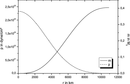
Figure 1: The mass $m(r)$ and the pressure $p(r)$ for a non–relativistic white dwarf with a central pressure of $p_{0}=2.2\cdot 10^{22}$ dyne/cm².

We will distinguish between the relativistic case and the non–relativistic case by setting $\gamma=4/3$ and $\gamma=5/3$, respectively. Choosing for the central pressure $p_{0}=2.33002\cdot 10^{22}{\ \rm dyne/cm^{2}}$, where this value satisfies the condition $k_{F}\ll m_{e}c$ (cf. eq. (24)), our numerical calculation with the Newtonian Code gives us the curve shown in Fig. 1 for the pressure–radius and the mass–radius relations. The white dwarf’s mass is $M=0.40362\ {\rm M_{\odot}}$ and the radius $R=10,919$ km.

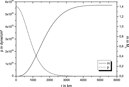
Figure 2: The mass $m(r)$ and the pressure $p(r)$ for a relativistic white dwarf with a central pressure of $p_{0}=5.62\cdot 10^{25}{\ \rm dyne/cm^{2}}$.

To satisfy the condition $k_{F}\gg m_{e}c$ for a relativistic white dwarf, we have to choose a larger central density compared to the non–relativistic case, $p_{0}=5.619\cdot 10^{25}$ dyne/cm² is an appropriate value (see Fig. 2).

There is one interesting point as far as the relativistic polytrope is concerned. As we have seen in section II.1.3 the mass limit to a white dwarf must be 1.4312 ${\rm M_{\odot}}$ if we set $\eta$ equal 2 and use a relativistic polytropic form for our equation of state. As these are exactly the same underlying assumptions as in our numerical computation, the maximum calculated mass must necessarily be the Chandrasekhar mass. Indeed, our numerical calculation gives us a white dwarf with a radius of 5710 km and a mass of 1.43145 M_⊙. With the chosen high initial pressure value we hit the Chandrasekhar mass limit very well.

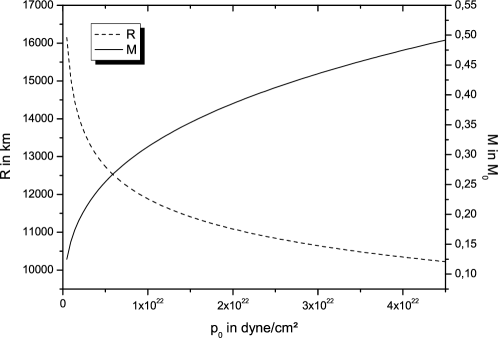
Figure 3: Calculated masses and radii for white dwarfs using the non–relativistic polytrope.

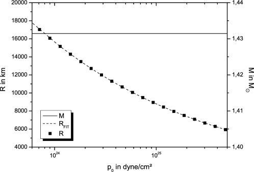
Figure 4: Calculated masses and radii for white dwarfs using the relativistic polytropic EoS.

Note, however, that according to the expression (53) the mass does not depend on the central pressure. To see this in more detail we have employed different central pressures: Fig. 4 shows the calculated masses of white dwarfs for initial pressures from $1\cdot 10^{23}{\ \rm dyne/cm^{2}}$ to $2.5\cdot 10^{24}{\ \rm dyne/cm^{2}}$. For this range of central pressures we always compute the same mass of 1.43145 ${\rm M_{\odot}}$. Hence, the numerical calculations agree with theory. As an additional check we also plot the corresponding radii which we computed numerically (points referred to as ”R”) and calculated analytically with eq. (50) (referred to as ”${\rm R_{FIT}}$”). The deviations of the numerically computed radii from the analytical ones are about 0.2%. Taking a look at the plot, we find that for increasing central pressure the mass of the relativistic white dwarf stays constant while the corresponding radius decreases. The behaviour of the mass and radius of a non–relativistic white dwarf with smaller central pressures is shown in Fig. 3 for comparison. In contrast to the relativistic case the mass increases now with increasing central pressures.

Silbar and Reddy already pointed out in Silbar and Reddy (2004) that the two polytropic white dwarf models examined here are not quite physical, as the non–relativistic EoS just works for central pressures below a certain threshold while the relativistic EoS is not applicable for small pressure. They suggest finding an EoS which covers the whole range of pressures by describing the energy density as a combination of a relativistic and a non–relativistic polytrope. We decided to try another way. On the other hand, we will employ not a guessed combination but a consistent relation ${p(\epsilon)}$.

II.2.3 Looking for zero–points

We remind the reader that it is our goal to find a relation between the energy density and the pressure which is needed for the calculation of the mass and the radius of the star. In the following, we want to use the full equations for a degenerate electron gas to derive the EoS consistently for the whole pressure range considered for white dwarfs. As we see from eqs. (20) and (24), it is impossible to write explicitly the energy density as a function of the pressure without using certain approximations on $\epsilon$ or p just like it was done in the previous section (i.e. the polytropic approximation).

On the other hand, a numerical solution to this problem is straight forward. As both the pressure and the energy density are functions of the Fermi momentum, we just have to find for a given pressure the corresponding Fermi momentum and use it in the equation for the energy density. With this procedure we are able to calculate the energy density $\epsilon$ for a given pressure $p$. To get the Fermi momentum we apply a root–finding method for the equation

$$p(k_{F})-p=0,$$ (63)

where $p$ is given and $p(k_{F})$ taken from eq. (24). As long as we have a simple expression for the derivative of pressure we use the Newton–Raphson–Method. In other cases, when we have more complicated equation of states, we take a simple bisection method, which is less accurate, but easier to handle. In addition, we write the energy density as the sum of the nucleon energy density and the electron energy density (in the polytropic approximation the energy density of the electrons was ignored). Employing this numerical prescription to the solution for the EoS, we can calculate the mass/pressure and the radius/pressure dependence, just like in the polytrope case.

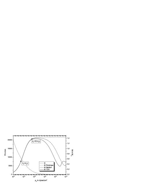
Figure 5: Calculated masses and radii for white dwarfs using a consistent EoS.

In section II.1.4 we discussed the corrections from general relativity and we will now test their influence on the masses and radii of white dwarfs. Fig. 5 shows our calculations for three different cases. In the case referred to as ”Polytrope” the energy density is given by just the nucleons, like in the polytropic EoS earlier. The ”Newton” mass/pressure curve is calculated with an energy density consisting of both, the nucleon and the electron energy density (see eq. (18)), for the ”TOV” curve the EoS is like the one for ”Newton” but with corrections from general relativity (eq. (55)). All three curves confirm the Chandrasekhar mass limit.

For pressures smaller than $10^{27}{\ \rm dyne/cm^{2}}$ the three cases are indistinguishable while for larger pressures the curves start to deviate significantly from each other. We have indicated two points on the mass/pressure curves: the first one corresponds to a central pressure where $k_{F}=m_{e}c$, i.e. the point where the electrons start to become relativistic, the second point is at $k_{F}=10m_{e}c$ and marks a central pressure where the electrons are highly relativistic. At the latter point, one can already see how the three curves start to deviate from each other. The similar behaviour for low pressure is due to the fact, that the electron contribution to the energy density as well as the corrections from general relativity are negligible. This is the non–relativistic region and the behaviour of the curves is comparable to the one of the non–relativistic polytrope ($p\propto\epsilon^{5/3}$), the mass increases with the central pressure.

The difference of the three curves in Fig. 5 starts to appear around $p_{0}=10^{27}{\ \rm dyne/cm^{2}}$ where $k_{F}=10m_{e}c$. Nevertheless, in all three cases the masses stay almost constant at a value of about $1.4\ {\rm M_{\odot}}$ around $p_{0}=10^{28}{\ \rm dyne/cm^{2}}$. At this pressure the relativistic electrons dominate the mass/pressure relation like in the relativistic polytrope case ($p\propto\epsilon^{4/3}$).

We will discuss the behaviour at larger pressure starting with the case ”Polytrope”. As the energy density for this model stems solely from the nucleons, the results for mass and radius for higher pressures have to merge into that of the relativistic polytrope. This is confirmed by the constant mass of 1.4314 solar masses (equal to the Chandrasekhar mass) for central densities above $p_{0}=10^{31}{\ \rm dyne/cm^{2}}$. The mass in the center of the white dwarfs increases with larger central densities while the radius decreases, such that the total mass stays constant.

For high pressures the contribution of the relativistic electrons to the energy density becomes important which is taken into account in the ”Newton” case. The EoS for electrons only can be approximated by an ultra–relativistic polytrope (see eq. (36)):

$$p=\frac{1}{3}\epsilon\quad.$$ (64)

With increasing central pressure the range in radius of the white dwarf where the electrons obey the ultra–relativistic limit enlarges. The deviation from the ”polytrope”–curve is an effect of the growing fraction of ultra–relativistic electrons. The masses for high pressures are now smaller than the ones in the ”Polytrope” case for the following reason: the degeneracy pressure of electrons for the same energy density will be lower in the ultra–relativistic polytrope compared to the ”Polytrope” case due to additional contribution of electrons to the energy density. Hence, the star will support less mass and the mass decreases as a function of pressure beyond the maximum mass. For the ”TOV” mass/pressure curve we take the former case adding effects from general relativity (see eq. (55)). At a pressure of $p_{0}\sim 10^{28}{\rm{dyne/cm^{2}}}$ the mass curve of white dwarfs exhibits a clear maximum with a maximum mass being a little bit lower than for the Newtonian cases i.e. $M_{max}=1.39\ {\rm M_{\odot}}$. The slightly reduced maximum mass is in accord with the fact that the corrections from general relativity strengthen the gravitational force. With increasing central pressures and smaller radii, corrections become larger. Therefore, the mass of the white dwarf decreases with increasing central pressures up to a pressure of about $p_{0}=2\cdot 10^{37}{\ \rm dyne/cm^{2}}$, here the mass starts to rise to a maximum value of about 0.51 solar masses and then decreases again. The general relativistic corrections applied in the ”TOV”–curve enhance the gravitational force, so that less mass is needed to create the given central pressure.

Figure 6: The mass–radius relation for white dwarfs with corrections for general relativity.

Fig. 6 shows the calculated masses for the ”TOV” case in dependence of the radius. The central pressure increases along the curve starting from the right to the left in the plot. The curve begins at large radii and small masses and continues to smaller radii and larger masses. Passing the maximum mass the curve starts to decrease with radius. For higher central pressures the curve starts to curl. This behaviour is typical for large central pressures, seen also in many other mass–radius relations for different equations of state. A detailed analysis of this curled shape can be found in Harrison (1965) and Harrison et al. (1965).

In the next subchapter we will discuss that white dwarfs of the ”Newton” and ”TOV” case which are beyond the maximum mass limit (i.e. for $p\gg p_{0}$) are unstable. It can be shown that polytropic equations of state with an exponent less than $4/3$ cause an instability (see e.g. Shapiro and Teukolsky (1983)): an increase in energy density causes an insufficient increase in pressure to stabilise the star.

II.2.4 Stability

First we argue that white dwarfs are unstable if $dM/dp_{0}<0$ following Glendenning (2000). For our argumentation we employ the mass curve in Fig. 7 and reason at first why white dwarfs with $p_{0}\leq p_{0}^{max}=p_{0}(M=M_{max})$ are stable.

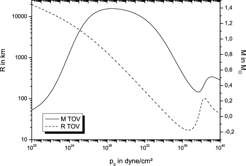
Figure 7: Calculated masses and radii for white dwarfs with corrections for general relativity

Let us assume that a white dwarf oscillates radially and therefore increases his central pressure to $p_{0}^{\prime}=p_{0}+\delta p_{0}$ with $\delta p_{0}>0$. In Fig. 7 the mass curve shows white dwarfs in hydrostatic equilibrium i.e. the degeneracy pressure and the gravitational force compensate each other. If for $p_{0}\leq p_{0}^{max}$ the central pressure is increased, the white dwarfs are only in hydrostatic equilibrium if their masses are larger than before. Since this is not the case, the surplus in degeneracy pressure over the gravitational attraction will expand the star back to his former state. For pressures $p_{0}^{\prime}=p_{0}-\delta p_{0}$ Fig. 7 shows that the mass $M(p_{0}^{\prime})$ of a white dwarf in hydrostatic equilibrium is smaller than $M(p_{0})$. That means that if the star expands due to radial oscillations the resulting lower central pressure can only be maintained if the gravitational force, i.e. the mass, decreases. As the mass of the white dwarf does not change the star has to shrink again to its former state. Therefore, white dwarfs with $p_{0}\leq p_{0}^{max}$ and $dM/dp_{0}>0$ are stable.

Now we discuss the situation for a white dwarf with $p_{0}>p_{0}^{max}$ and $dM/dp_{0}<0$. If the central pressure is lowered to $p_{0}^{\prime}=p_{0}-\delta p_{0}$ then $M(p_{0}^{\prime})$ should be larger than $M(p_{0})$ to bring the star in hydrostatic equilibrium (see Fig. 7). So the gravitational force is not large enough to stop the expansion and the white dwarf is unstable to radial oscillations. For an increased central pressure $p_{0}^{\prime}=p_{0}+\delta p_{0}$ the mass curve shows that stability is only given for a white dwarf with $p_{0}\leq p_{0}^{max}$. As the mass of the white dwarf is larger than the one required for hydrostatic equilibrium, gravitation will cause the white dwarfs to shrink and finally to collapse.

In Harrison et al. (1965), Weber (1999) as well as in Shapiro and Teukolsky (1983), which we will follow now, a more formal approach is presented. Again, one considers radial oscillations of the white dwarf. The radial modes $\omega_{n}$ can be derived by solving a Sturm–Liouville eigenvalue equation with the eigenvalues ${\omega_{n}}^{2}$. In doing so one gets a range of eigenvalues with

$${\omega_{0}}^{2}<{\omega_{1}}^{2}<{\omega_{2}}^{2}<...$$ (65)

where $\omega_{n}$ are the eigenfrequencies to the radial modes and $\omega_{0}$ corresponds to the fundamental radial mode. For the instability analysis the so called ”Lagrangian displacement” $\xi$ (x,t) is introduced in ref. Shapiro and Teukolsky (1983) which connects fluid elements in the unperturbed state to corresponding elements in the perturbed state. The normal modes of an oscillation can then be written as

$$\xi^{i}(\textbf{x},t)=\xi^{i}(\textbf{x})e^{i\omega t}\quad,$$ (66)

where $\xi^{i}$ are any Lagrangian displacements. Hence, the star will be stable for $\omega^{2}\geq 0$ and unstable for $\omega^{2}<0$. This means that for stability all modes need to have real eigenfrequencies. But because of (65) the stability of the star depends only on the sign of ${\omega_{0}}^{2}$.

The instability condition can be connected to the total Mass of any single star in in hydrostatic equilibrium (i.e. every star lying on our $M(R)$ curve). The variation $\delta M$ of the mass out of the state of equilibrium can be expressed as follows:

$$M=M_{0}+\delta M+\delta^{2}M\quad,$$ (67)

where $M_{0}$ is the total mass at equilibrium. For all stars in hydrostatic equilibrium it holds that the variation $\delta M=0$. It can be shown (see Shapiro and Teukolsky (1983)) that stability is given for $\delta^{2}M>0$ with an onset of instability at $\delta^{2}M=0$. For $\delta^{2}M<0$ the star is unstable. In the mass/pressure relation one finds minima and maxima, where $dM/dp_{0}=0$. For these extrema it can be deduced that also $\delta^{2}M=0$. This means these extrema are the critical points for stability. The latter condition relates to $\omega^{2}=0$ and therefore signals a change in the stability of the corresponding normal mode.

In the case of multiple critical points it is also possible that an unstable configuration can change back to stability at the following extremum. Therefore one has to take into account the sign of the change in the radius R (i.e. $dR/dp_{0}<0$ or $dR/dp_{0}>0$) in addition. If an equilibrium configuration of a star is now transformed from the low–pressure side of the critical point to the high–pressure side, one can find the following relations between the change of the radius $R$ with respect to the central pressure $p_{0}$ and the radial oscillation modes:

• $dR/dp_{0}<0$: the square of the oscillation frequency of an even numbered mode changes the sign (${\omega_{n}}^{2}\rightarrow-{\omega_{n}}^{2}$)

• $dR/dp_{0}>0$: the square of the oscillation frequency of an odd numbered mode changes the sign.

For the ”TOV” curve in Fig. 5 there are three critical points. The first critical point appears at the maximum around $p_{0}=10^{28}{\ \rm dyne/cm^{2}}$. As can be seen in Fig. 7 $dR/dp_{0}$ is negative in this critical point, therefore an even mode is changing stability. Because of (65) and the assumption that for low densities the ocsillation frequencies of all modes are real (i.e. ${\omega_{n}}^{2}>0$), ${\omega_{0}}^{2}$ should change its sign here. Therefore, for central pressures between the first critical point and the next one, the oscillation in the fundamental mode is unstable.

At $p_{0}\sim 10^{37.5}{\ \rm dyne/cm^{2}}$, the second critical point is reached. Here $dR/dp_{0}>0$ and ${\omega_{1}}^{2}$ becomes negative. At the second maximum at $p_{0}\sim 10^{39}{\ \rm dyne/cm^{2}}$ again the oscillation in an even mode must change the sign and as ${\omega_{1}}^{2}$ is negative already, ${\omega_{2}}^{2}$ becomes negative now. This stability analysis can also be applied to the case of the Newtonian white dwarfs as well as to the neutron stars. As mentioned before, the sequence can become stable again; then at the second critical point the fundamental mode changes its sign back and a stable sequence of compact stars starts again. This so called third family of compact stars appears for a strong first order phase transition to e.g. quark matter Gerlach (1968); Glendenning and Kettner (2000); Schertler et al. (2000).

In summary white dwarfs become unstable as soon as their mass is above the Chandrasekhar mass limit. This is exactly what is happening in the case of a core collapse supernova explosion. It is quite interesting to see that such an intuitive reasoning already indicates what is happening in real nature.

III Pure Neutron Stars

III.1 Non–relativistic polytropic case

In this chapter we start looking at pure non–relativistic neutron stars, which are described by an EoS of a Fermi gas of neutrons. In the following we drop the subscript $F$ for labelling the Fermi momentum due to practical reasons. With the neutron number density

$$n_{n}=\frac{k_{n}^{3}}{3\pi^{2}\hbar^{3}}$$ (68)

and the mass density

$$\rho=n_{n}\cdot m_{n}$$ (69)

we get in analogy to the Fermi gas for electrons (see eqs. (19) – (24)):

$$\epsilon(x) = \frac{\epsilon_{0}}{8}[(2x^{3}+x)(1+x^{2})^{1/2}-\sinh^{-1}(x)]$$ (70)

$$p(x) = \frac{\epsilon_{0}}{24}[(2x^{3}-3x)(1+x^{2})^{1/2}+3\sinh^{-1}(x)]$$ (71)

with

$$x=\frac{k_{n}}{m_{n}c},\quad\epsilon_{0}=\frac{m_{n}^{4}c^{5}}{\pi^{2}\hbar^{3}}\quad.$$ (72)

In the non–relativistic case eqs. (70) and (71) simplify to:

$$\epsilon(x)\simeq\rho c^{2}=\frac{\epsilon_{0}}{3}x^{3},\quad p(x)\simeq\frac{\epsilon_{0}}{15}x^{5}.$$ (73)

Hence, the EoS can be described by a polytrope:

$$p(\epsilon)=K_{nrel}\epsilon^{5/3}$$ (74)

with

$$K_{nrel}=\frac{\hbar^{2}}{15\pi^{2}m_{n}}\left(\frac{3\pi^{2}}{m_{n}c^{2}}\right)^{5/3}=6.428\cdot 10^{-26}\ \frac{{\rm cm}^{2}}{{\rm erg}^{2/3}}\quad.$$ (75)

We start our numerical calculation with our Newtonian code and the results are plotted in Fig. 8. We arrive at neutron star masses of around 0.5 M_⊙ and radii of 20 km to 30 km. The general relativistic effects for neutron stars should be larger than for the white dwarfs. In Fig. 8 we compare the Newtonian with the TOV–code results. We see that the general relativistic corrections are at the order of a few percent and become more and more pronounced for more massive neutron stars.

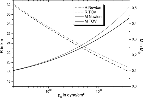
Figure 8: The mass $M$ and radius $R$ of neutron stars in the non–relativistic case as a function of the central pressure $p_{0}$. The results from the TOV equation are compared to the Newtonian limit.

III.2 Ultra–relativistic polytropic case

For the ultra–relativistic limit, $x\gg 1$, one finds for the energy density and for the pressure of nucleons:

$$\epsilon(x)=\frac{\epsilon_{0}}{4}x^{4}\quad,\qquad p(x)=\frac{\epsilon_{0}}{12}x^{4}\Rightarrow\quad p=\epsilon/3$$ (76)

which is similar to the case of ultra–relativistic electrons discussed before. However, the numerical integration of the TOV equations fails here: The condition for terminating the integration ($p\leq 0$) can not be reached. The pressure converges monotonically as a function of the radius against zero, so that the radius of the star approaches infinity. The mass does not go to infinity because $dm/dr$ also reaches zero asymptotically. The problem with the relativistic case is, that its solution has some principal inconsistencies. Running from the initial pressure $p_{0}$ to zero through the whole star, the pressure has to pass the region where neutrons become non–relativistic, necessarily. The pure relativistic approximation is not valid for the whole density range of a compact star.

III.3 Full relativistic case

It is essentially to find an equation of state which is valid over the whole range of pressure and energy density. In other words: Eqs. (70) and (71) should be used for the calculation. Again we use a root–finding routine, as we have no explicit equation of state of the form $p(\epsilon)$ or $\epsilon(p)$ any more. The results for $R(p_{0})$ and $M(p_{0})$ are shown in Fig. 9.

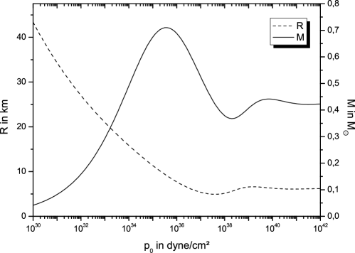
Figure 9: Mass $M$ and radius $R$ as a function of the central pressure $p_{0}$ for pure neutron stars.

Figure 10: The mass $M$ for pure neutron stars as a function of radius $R$. The maximum mass is $M=0.712$ M_⊙ at a radius of $R=9.14$ km.

The mass–radius relation $M(R)$ is plotted in Fig. 10, where the maximum mass can be easily recognised. The heaviest stable pure neutron star has a central pressure of $p_{0}=3.5\cdot 10^{35}$ dyne/cm², a mass of $M=0.712$ M_⊙ and a radius of $R=9.14$ km as first calculated by Oppenheimer and Volkoff in 1939 Oppenheimer and Volkoff (1939) (they arrived at a maximum mass of $M=0.71$ M_⊙ and a radius of $R=9.5$ km for comparison).

IV Neutron Stars with Protons and Electrons

Because the neutron is unstable, a neutron star will not consist of neutrons only, but in addition a finite fraction of protons and electrons will appear in dense matter. The electrons and protons are produced by $\beta$–decay:

$$n\longrightarrow p+e^{-}+\bar{\nu}_{e}.$$ (77)

There exist reverse reactions also, so that an electron and a proton scatter into a neutron and a neutrino:

$$p+e^{-}\longrightarrow n+\nu_{e}.$$ (78)

As all reactions are in chemical equilibrium, for a cold neutron star, the following relation for the chemical potentials holds:

$$\mu_{n}=\mu_{p}+\mu_{e}.$$ (79)

Neutrinos do not have a finite chemical potential ($\mu_{\nu}=0$), as the neutrinos escape from the cold star without interactions. Due to stability reasons (see e.g. Glendenning (2000)), it is assumed that the whole neutron star is electrically neutral, hence:

$$n_{p}=n_{e}\Leftrightarrow k_{p}=k_{e}$$ (80)

and the Fermi momenta of protons and electrons must be equal. With the definition of the chemical potential for an ideal Fermi gas with zero temperature,

$$\mu_{i}(k_{i})=\frac{d\epsilon_{i}}{dn_{i}}=(k_{i}^{2}c^{2}+m_{i}^{2}c^{4})^{1/2},\quad i=n,p,e,$$ (81)

and using eqs. (79) and (80), one arrives at the following relation:

$$(k_{n}^{2}c^{2}+m_{n}^{2}c^{4})^{1/2}-(k_{p}^{2}c^{2}+m_{p}^{2}c^{4})^{1/2}-(k_{p}^{2}c^{2}+m_{e}^{2}c^{4})^{1/2}=0.$$ (82)

This equation can be solved for the Fermi momenta of protons $k_{p}$ as a function of the Fermi momenta of neutrons $k_{n}$:

$$k_{p}(k_{n})=\frac{[(k_{n}^{2}c^{2}+m_{n}^{2}c^{4}-m_{e}^{2}c^{4})^{2}-2m_{p}^{2}c^{4}(k_{n}^{2}c^{2}+m_{n}^{2}c^{4}+m_{e}^{2}c^{4})+m_{p}^{4}c^{8}]^{1/2}}{2c(k_{n}^{2}c^{2}+m_{n}^{2}c^{4})^{1/2}}\quad.$$ (83)

The total energy and the pressure are now the sum of the energy and pressure of electrons, protons and neutrons, respectively:

$$\epsilon_{tot}=\sum_{i=n,p,e}\epsilon_{i}\,,\quad p_{tot}=\sum_{i=n,p,e}p_{i},$$ (84)

where

$$\epsilon_{i}(k_{i}) = \frac{8\pi}{(2\pi\hbar)^{3}}\int_{0}^{k_{i}}(k^{2}c^{2}+m_{i}^{2}c^{4})^{1/2}k^{2}dk$$ (85)

$$p_{i}(k_{i}) = \frac{1}{3}\frac{8\pi}{(2\pi\hbar)^{3}}\int_{0}^{k_{i}}(k^{2}c^{2}+m_{i}^{2}c^{4})^{-1/2}k^{4}dk.$$ (86)

For the case when there are no neutrons present, i.e. $k_{n}=0$, eq. (83) gives:

$$k_{p}(0)=\frac{[(m_{n}^{2}c^{4}-m_{e}^{2}c^{4})^{2}-2m_{p}^{2}c^{4}(m_{n}^{2}c^{4}+m_{e}^{2}c^{4})+m_{p}^{4}c^{8}]^{1/2}}{2m_{n}c^{3}}=1.264\cdot 10^{-3}m_{n}c.$$ (87)

This means, that eq. (83) can only be used, if $k_{p}>1.264\cdot 10^{-3}m_{n}c$, which is fulfilled for $p>p_{\rm crit}=3.038\cdot 10^{24}{\ \rm dyne/cm^{2}}$. Below this pressure, no neutrons are present any more, so the ”neutron star” material consists of protons and electrons only. Fig. 11 shows the equation of state for a free gas of protons, electrons and neutrons in $\beta$–equilibrium in the form $\epsilon(p)$. Around the critical pressure, a notable kink appears in the equation of state, which can be identified with the strong onset of neutrons appearing in matter with their corresponding additional contribution to the energy density. (One can show that $\left.\frac{d^{2}\epsilon}{dp^{2}}\right|_{p_{\rm crit}}=\infty$, but $\left.\frac{d\epsilon}{dp}\right|_{p_{crit}}$ is continuous and thus the physical situation is not that of a true thermodynamic phase transition.)

Figure 11: The energy density $\epsilon$ as a function of the pressure $p$ for neutron stars including protons and electrons. At $p=3\cdot 10^{24}{\ \rm dyne/cm^{2}}$ neutrons begin to appear.

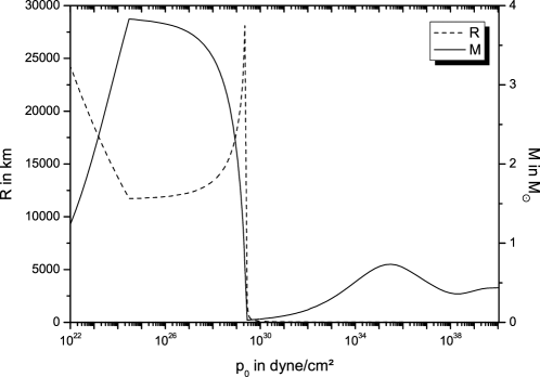
Figure 12: Mass $M$ and radius $R$ as a function of the central pressure $p_{0}$ for neutron stars including protons and electrons.

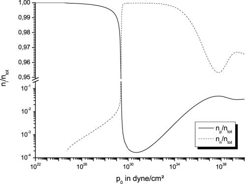
Figure 13: The proton to nucleon fraction $n_{p}/n_{tot}$ and the neutron to nucleon fraction $n_{n}/n_{tot}$, integrated over every single star, versus the central pressure $p_{0}$.

Figure 14: The Mass $M$ as a function of the radius $R$ for neutron stars including protons and electrons. The maximum mass star has a mass of $M=0.699{\ \rm M_{\odot}}$, the corresponding radius is $R=9.24$ km.

Using the new equation of state, we start our TOV calculation and compute masses and radii which are depicted in Fig. 12 and Fig. 14, respectively. The result seems to be surprising at a first glance but can be explained by looking at the proton to nucleon fraction integrated over every single star as displayed in Fig. 13.

Below the critical pressure of $p=3.038\cdot 10^{24}{\ \rm dyne/cm^{2}}$, the neutron star consists of protons and electrons only by definition. Above this pressure, neutrons appear, resulting in a sharp bend of $M(p_{0})$ and $R(p_{0})$. Between the critical pressure and $p\simeq 10^{29}{\ \rm dyne/cm^{2}}$, the stars have a tiny neutron fraction in the core, which increases with the pressure. The increasing neutron fraction is responsible for the decreasing masses. On the microscopic scale the relativistic electrons combine with the protons to form neutrons, thereby reducing the electron degeneracy pressure. For the same energy density the pressure will be lower, if neutron production is included, so only a smaller mass is supported by the star. At $p\simeq 10^{30}{\ \rm dyne/cm^{2}}$ the proton fraction drops to $n_{p}/n_{tot}\leq 10^{-3}$ and the star becomes an almost pure neutron star (hence the name). The proton fraction is so small, that it can be safely neglected. As a consequence the stellar objects become more compact, with a smaller radius and mass. For larger pressures ($p>10^{30}{\ \rm dyne/cm^{2}}$), the mass increases again with rising pressure. The neutrons start to become degenerate, the star is stable because of the neutron degeneracy pressure.

Figure 15: The pressure $p$ along the radius $r$ for a single neutron star including protons and electrons at $p_{0}=2\cdot 10^{29}{\ \rm dyne/cm^{2}}$.

So the behaviour of $M(p_{0})$ is understood through the change of the proton fraction $n_{p}/n_{tot}(p_{0})$. But what about the unusual peak of $R(p_{0})$? Similar to the ultra–relativistic description of a pure neutron star, the situation at $p_{0}\simeq 10^{29}{\ \rm dyne/cm^{2}}$ is, that the pressure approaches zero very slowly, but never reaches it or falls below. Fig. 15 shows a star with $p_{0}=2\cdot 10^{29}{\ \rm dyne/cm^{2}}$, where this behaviour can be clearly seen. So it is necessary to make a cut–off (for this case at $p=10^{19}{\ \rm dyne/cm^{2}}$), so that the integration terminates as soon as this pressure is reached. During the numerical computation the mass converges to $M$, while the radius grows bigger and bigger. This neutron star consists of a dense central core and a huge low–density crust. The protons and electrons are responsible for these huge radii: the energy density for the same pressure is much lower, if no neutrons are present (see Fig. 11). Because $dp/dr$ (eq. (55)) is a function of the energy density $\epsilon$, the pressure $p(r)$ inside a star will decrease much slower, if there are only protons and electrons left. For more massive stars this crust disappears and the radius is determined by the neutron core. After all, such a huge crust does not seem to be very realistic for neutron stars.

Note that for the most compact neutron stars (i.e. for $p_{0}>10^{34}{\ \rm dyne/cm^{2}}$) protons appear again. The proton fraction approaches a certain constant limit at high densities. Using eq. (83) in the ultra–relativistic limit, $k_{n}c\gg m_{n}c^{2}$, results in:

$$k_{p}(k_{n})\approx 1/2k_{n}\Longrightarrow n_{p}=1/8n_{n}$$ (88)

$$\Longrightarrow\frac{n_{p}}{n_{tot}}=\frac{n_{p}}{n_{p}+n_{n}}=\frac{1}{9}\quad.$$ (89)

The proton fraction for large $p_{0}$ in Fig. 13 is of course smaller than 1/9, as only the central core obeys the relativistic limit, and no protons are present for the regions in the star with smaller pressure. The maximum mass star has a proton fraction of $n_{p}/n_{tot}\simeq 0.02$.

Another important point is, that all stars in the region of $10^{24}{\ \rm dyne/cm^{2}}<p_{0}<10^{29}{\ \rm dyne/cm^{2}}$ are unstable, which can be seen from the $M$ versus $p_{0}$ plot in Fig. 12. Hence, there are only two different kinds of stable objects: first the ”hydrogen white dwarfs”, like stars consisting of protons and electrons, up to $M=4{\ \rm M_{\odot}}$ and radii of about $10^{4}$ km, then the almost pure neutron stars with a maximum mass of $M=0.699{\ \rm M_{\odot}}$ and a radius $R=9.24$ km at a central pressure $p_{0}=3.412\cdot 10^{35}{\ \rm dyne/cm^{2}}$. Compared to $M=0.712{\ \rm M_{\odot}}$ and $R=9.14$ km for the pure neutron star of the last section, the differences are quite small. The minimum neutron star mass is found to be about $0.03M_{\odot}$ with a radius of around 1000 km; the radius rapidly changes for this mass range and quickly shrinks to values of 200–300 km for slightly larger masses. We note that these values for the minimum mass of neutron stars are not far from the result of $M_{\rm min}=0.09M_{\odot}$ found in more elaborate calculations (see e.g. Haensel et al. (2002)).

V Models for the nuclear interactions

V.1 Empirical interaction

In this and the following section we use MeV and fm for the energy and distance units. Additionally $c$ is set to 1 and $\hbar c=197.3$ MeV fm.

Following Silbar and Reddy (2004), we introduce an empirical interaction for symmetric matter ($n_{n}=n_{p}$) of the form (see also Prakash et al. (1988)):

$$\frac{\epsilon(n)}{n}=m_{N}+\left<E_{0}\right>u^{2/3}+\frac{A}{2}u+\frac{B}{\sigma+1}u^{\sigma},\quad u=n/n_{0}\quad.$$ (90)

The dimensionless quantity $\sigma$, and the quantities $A$ and $B$ with dimension of MeV, are the fit parameters of the model. In fact, only the third and the fourth term of eq. (90) describe interaction terms, $\left<E_{0}\right>$ is the average kinetic energy per nucleon of symmetric matter in its ground state:

$$\left<E_{0}\right>=\frac{3}{5}\frac{k_{0}^{2}}{2m_{N}}=\frac{3}{5}\frac{1}{2m_{N}}\left(\frac{3\pi^{2}\hbar^{3}n_{0}}{2}\right)^{2/3}\quad.$$ (91)

The factor two in the denominator of the parenthesis comes in as an additional degeneration factor for the isospin (compare to eq. (15)).

In the model the following values should be reproduced by the ansatz of eq. (90):

• the equilibrium number density $n_{0}=0.16{\ \rm nucleons/fm^{3}}\Longrightarrow k_{0}=263{\ \rm MeV}$

• the average binding energy per nucleon $BE=\left.(E/A-m_{N})\right|_{n=n_{0}}=\left.(\epsilon(n)/n-m_{N}\right)|_{n=n_{0}}=-16{\ \rm MeV}$

• the nuclear compressibility in nuclear matter $K(n_{0})=\left.9\frac{dp(n)}{dn}\right|_{n=n_{0}}=400{\ \rm MeV}$

After some algebra one gets the following parameters:

$$A=-118.2{\ \rm MeV},\quad B=65.39{\ \rm MeV},\quad\sigma=2.112,\quad\left<E_{0}\right>=22.1{\ \rm MeV}.$$ (92)

For known $\epsilon(n)$ it is possible to determine $p(n)$ via:

$$p(n)=n^{2}\frac{d}{dn}\left(\frac{\epsilon}{n}\right)=n_{0}\left[\frac{2}{3}\left<E_{0}\right>u^{5/3}+\frac{A}{2}u^{2}+\frac{B\sigma}{\sigma+1}u^{\sigma+1}\right]\quad.$$ (93)

We proceed now to extrapolate to asymmetric nuclear matter.

First, the neutron to proton ratio is expressed through a parameter $\alpha$:

$$\alpha=\frac{n_{n}-n_{p}}{n}=\frac{N-Z}{A}\quad.$$ (94)

Now the kinetic energy is given by the sum of the kinetic energies of protons and neutrons:

$$\epsilon_{KE}(n,\alpha) = \frac{3}{5}\frac{k_{n}^{2}}{2m_{N}}\,n_{n}+\frac{3}{5}\frac{k_{p}^{2}}{2m_{N}}\,n_{p}$$ (95)

$$= n\left<E_{F}\right>\frac{1}{2}\left[\left(1+\alpha\right)^{5/3}+\left(1-\alpha\right)^{5/3}\right],$$ (96)

$$\left<E_{F}\right> = \frac{3}{5}\frac{1}{2m_{N}}\left(\frac{3\pi^{2}\hbar^{3}n}{2}\right)^{2/3}\quad.$$ (97)

The difference in the kinetic energy density relative to the symmetric case can be expressed as a function of $n$ and $\alpha$:

$$\Delta\epsilon_{KE}(n,\alpha) = \epsilon_{KE}(n,\alpha)-\epsilon_{KE}(n,0)$$ (98)

$$= n\left<E_{F}\right>\left\{\frac{1}{2}\left[\left(1+\alpha\right)^{5/3}+\left(1-\alpha\right)^{5/3}\right]-1\right\}\quad.$$

This gives the following Taylor–Approximation:

$$\Delta\epsilon_{KE}(n,\alpha)=n\left<E_{F}\right>\frac{5}{9}\alpha^{2}\left(1+\frac{\alpha^{2}}{27}+\cdots\right).$$ (99)

This motivates that it is sufficient to keep corrections of order $\alpha^{2}$:

$$\frac{E(n,\alpha)}{A}=\frac{E(n,0)}{A}+\alpha^{2}S(n).$$ (100)

The function $S(u)$, which describes the symmetry energy, is assumed to have the following form:

$$S(u)=(2^{2/3}-1)\left<E_{0}\right>\left(u^{2/3}-F(u)\right)+S_{0}F(u).$$ (101)

$S_{0}$ is an input parameter (the asymmetry energy), which describes the energy difference between pure neutron matter and normal symmetric nuclear matter at ground state density $n_{0}$. In the following calculations, $S_{0}$ is set to 30 MeV. The only restrictions to the function $F(u)$ are $F(1)=1$, and $F(0)=0$, in order to satisfy $S(1)=S_{0}$, and $S(0)=0$, respectively. Besides this, $F(u)$ can be chosen freely. We make the straight forward choice,

$$F(u)=u.$$ (102)

The factor $(2^{2/3}-1)\left<E_{0}\right>$ can be explained as follows: For pure neutron matter, $\alpha=1$, the kinetic energy is not given by eq. (91) any more, the factor 2 in the denominator of the parenthesis has to drop out. The factor $(2^{2/3}-1)\left<E_{0}\right>$ takes this into account:

$$\frac{E(n,1)}{A} = m_{N}+\left<E_{0}\right>u^{2/3}+\frac{A}{2}u+\frac{B}{\sigma+1}u^{\sigma}+(2^{2/3}-1)\left<E_{0}\right>\left(u^{2/3}-F(u)\right)+S_{0}F(u)$$ (103)

$$= m_{N}+\left<E_{0}\right>u^{2/3}+(2^{2/3}-1)\left<E_{0}\right>u^{2/3}+\frac{A}{2}u+\frac{B}{\sigma+1}u^{\sigma}+\left(S_{0}-(2^{2/3}-1)\left<E_{0}\right>\right)F(u)$$

$$= m_{N}+2^{2/3}\left<E_{0}\right>u^{2/3}+\frac{A}{2}u+\frac{B}{\sigma+1}u^{\sigma}+\left(S_{0}-(2^{2/3}-1)\left<E_{0}\right>\right)F(u)$$

Thus the ansatz of eq. (101) implies the correct expression for the kinetic energy of pure neutron matter. Also the different contributions to the potential energy are separated from each other.

With $\epsilon(n,\alpha)=nE(n,\alpha)/A$ it is straightforward to calculate $p(n,\alpha)$:

$$p(n,\alpha) = n^{2}\frac{d}{dn}\left(\frac{\epsilon(n,\alpha)}{n}\right)$$ (104)

$$= p(n,0)+n_{0}\alpha^{2}\left[(2^{2/3}-1)\left<E_{0}\right>\left(2/3u^{5/3}-u^{2}\right)+S_{0}u^{2}\right].$$

As seen in the previous section, the proton fraction for stable compact stars is small. Hence, the parameter $\alpha$ is set to be equal 1 and a pure neutron star is considered in the following.

Figure 16: The mass $M$ as a function of the radius $R$ for the empirical nucleon–nucleon interaction. The maximum mass star has a mass of $M=2.792{\ \rm M_{\odot}}$, the corresponding radius is $R=12.46$ km.

With $p(n)$ and $\epsilon(n)$ given, one can start again the numerical computation. The results are shown in Fig. 16. The maximum mass star has a mass of $M=2.792{\ \rm M_{\odot}}$ and a radius of $R=12.46$ km. The neutron star is much more massive, if nucleon–nucleon interactions are included. As the equation of state is much harder, which means that the pressure increases faster with the energy density, the star can support a much larger mass.

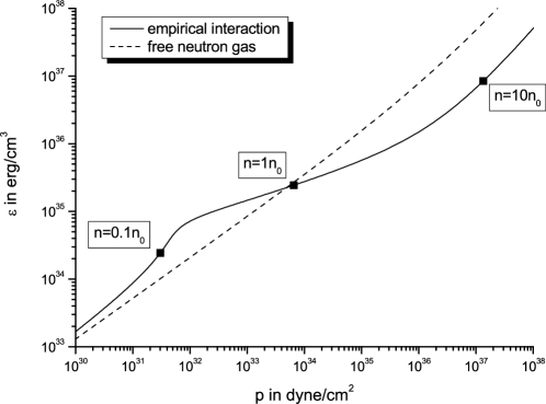
Figure 17: The equation of state for the empirical nucleon–nucleon interaction compared to the one of a free neutron gas.

Another interesting fact is the behaviour of the mass for decreasing central pressure. In a certain region the mass–radius curve drops to smaller radii as the pressure and the mass decrease, until a radius of $R\simeq 9.5$ km and a mass of $M\simeq 0.1{\ \rm M_{\odot}}$ is reached at a central pressure of $p\simeq 1.7\cdot 10^{33}{\ \rm dyne/cm^{2}}$. Passing this point, the radius starts to increase again. This special shape is due to the equation of state employed here. In Fig. 17 one sees that the EoS differs from the ones before: There is a smooth bump at $p\simeq 4\cdot 10^{31}{\ \rm dyne/cm^{2}}$. For pressures below this value an increase in the energy density leads to a very small increase in pressure, which is due to the attractive part of the interaction for matter close to the ground state density. In this pressure region a higher central pressure can only be generated by a smaller radius at a nearly unchanged mass. The slope of the EoS for pressures larger than the value of $p\simeq 4\cdot 10^{31}{\ \rm dyne/cm^{2}}$ changes noticeable, so that also the mass–radius relation for the corresponding neutron stars is affected. For larger pressures the pressure increases much faster with the energy density, which results in the abrupt rise of the masses (see Fig. 16). The repulsive force of the interaction becomes dominant for nuclear densities above ground state density. Now an increase in energy density leads to a strong increase in pressure also and a larger mass is supported by the star.

In fact, the EoS used here is not valid for small pressures and energy densities. Below nuclear matter density $n_{0}$ it is not realistic to use a uniform matter distribution anymore. The formation of a lattice of nuclei and the occurance of certain possible mixed phases become important in the outer layers, the so called crust of neutron stars. For pressures below $10^{33}{\ \rm dyne/cm^{2}}$ one has to use a special equation of state to describe the matter in the crust. Taking into account a realistic EoS for the crust would wash out the bump seen in Fig. 17 and also the characteristic features in the mass–radius relation described above. A good introduction to neutrons star crusts can be found in e.g. Baym et al. (1971) and Haensel (2001).

V.2 Skyrme parameterised interaction

In the following, the properties of nuclear matter are considered by applying the Hartree–Fock–method on a phenomenological nucleon–nucleon interaction taken from Greiner (2004) (for further information see also Ring and Schuck (2004)).

Consider a system consisting of $N_{p}$ protons and $N_{n}$ neutrons, which are described by plain waves:

$$\varphi_{{\alpha}}=\frac{1}{\sqrt[]{V}}e^{ikx}\chi_{S}\chi_{I}.$$ (105)

Here, $\chi_{I}$ is the degree of freedom for the isospin, $\chi_{S}$ for the spin. The self–consistent Hartree–Fock equations read:

$$\epsilon_{{\alpha}}\varphi_{{\alpha}}(x)=\hat{t}\varphi_{{\alpha}}(x)+\sum_{{\alpha^{\prime}}}\int d^{3}y\varphi_{{\alpha}}^{\dagger}(y)V(x,y)\left[\varphi_{{\alpha^{\prime}}}(y)\varphi_{{\alpha}}(x)-\varphi_{{\alpha}}(y)\varphi_{{\alpha^{\prime}}}(x)\right].$$ (106)

where $\sum_{{\alpha^{\prime}}}$ is the sum over all occupied states. The potential is spin– and isospin–independent, so the sum can be divided into a part for protons and one for neutrons:

$$\sum_{{\alpha^{\prime}}}...=\sum_{k,s}^{k_{F}^{(p)}}...+\sum_{k,s}^{k_{F}^{(n)}}$$ (107)

As the sum splits up, one gets a separate Hartree–Fock–equation for neutrons and protons:

$$\epsilon_{k}^{(p)}\varphi_{k}^{(p)}(x)=\hat{t}\varphi_{k}^{(p)}(x) + (2s+1)\sum_{k^{\prime}}^{k_{F}^{(p)}}\int d^{3}y[\varphi_{k^{\prime}}^{(p)*}(y)\varphi_{k^{\prime}}^{(p)}(y)]V(x,y)\varphi_{k}^{(p)}(x)$$ (108)

$$- 1\cdot\sum_{k^{\prime}}^{k_{F}^{(p)}}\int d^{3}y[\varphi_{k^{\prime}}^{(p)*}(y)\varphi_{k}^{(p)}(y)]V(x,y)\varphi_{k^{\prime}}^{(p)}(x)$$

$$+ (2s+1)\sum_{k^{\prime}}^{k_{F}^{(n)}}\int d^{3}y[\varphi_{k^{\prime}}^{(n)*}(y)\varphi_{k^{\prime}}^{(n)}(y)]V(x,y)\varphi_{k}^{(p)}(x).$$

by taking into account the spin–degrees of freedom $g_{s}=2s+1$. The neutron wave function results from replacing the superscript $(p)$ by $(n)$.

Next, the interaction is introduced as a Skyrme–type parameterisation:

$$V(x,y)=\delta^{3}(x-y)(\frac{1}{6}t_{3}n-t_{0}),$$ (109)

where $t_{0}$ describes the attractive two particle nuclear interaction, whereas $t_{3}n$ describes the repulsive (and density depended) many–body interaction which is the dominant one at high nuclear densities. Here, $n$ denotes the total number density of the system:

$$n=(N_{n}+N_{p})/V=n_{n}+n_{p}.$$ (110)

The single–particle–energies for protons and neutrons can then be derived to be:

$$\epsilon_{k}^{(p)} = \frac{k_{p}^{2}}{2m_{p}}+(\frac{1}{6}t_{3}n-t_{0})\frac{1}{V}(N_{p}/2+N_{n})$$

$$\epsilon_{k}^{(n)} = \frac{k_{n}^{2}}{2m_{n}}+(\frac{1}{6}t_{3}n-t_{0})\frac{1}{V}(N_{n}/2+N_{p}).$$ (111)

The total energy for a homogeneous system is given by:

$$E_{HF}=\frac{1}{2}\sum_{i}^{N_{p}}(\epsilon_{i}^{(p)}+t_{i})+\frac{1}{2}\sum_{i}^{N_{n}}(\epsilon_{i}^{(n)}+t_{i})$$ (112)

$$\Longrightarrow E_{HF}=N_{p}\frac{3}{5}\frac{k_{p}^{2}}{2m_{p}}+N_{n}\frac{3}{5}\frac{k_{n}^{2}}{2m_{n}}+\frac{1}{2}(\frac{1}{6}t_{3}n-t_{0})\frac{1}{V}(N_{p}^{2}/2+2N_{p}N_{n}+N_{n}^{2}/2).$$ (113)

The next task is to determine the phenomenological parameters $t_{0}$ and $t_{3}$. For $n=n_{0}=0.16{\ \rm fm^{3}}$ the total energy shall have a minimum with $E_{HF}/A=BE=-16$ MeV. From these conditions one arrives at:

$$t_{3} = \frac{16E_{B}}{n_{0}^{2}}+\frac{8}{5}\frac{(\hbar c)^{2}}{m_{n}c^{2}}\left(\frac{3\pi^{2}}{2}\right)^{2/3}(n_{0})^{-4/3}$$

$$t_{0} = \frac{16E_{B}}{3n_{0}}+\frac{16}{15}\frac{(\hbar c)^{2}}{m_{n}c^{2}}\left(\frac{3\pi^{2}}{2}\right)^{2/3}(n_{0})^{-1/3}$$ (114)

$$\Longrightarrow t_{0}=1024.1{\ \rm MeV\ fm^{3}},\quad\ t_{3}=14600.8{\ \rm MeV\ fm^{6}}\quad.$$ (115)

With

$$K(n_{0})=\left.9\frac{dp(n)}{dn}\right|_{n=n_{0}}\quad,$$ (116)

one finds a value of $376.4$ MeV for the nuclear compressibility, which is less than for the empirical interaction.

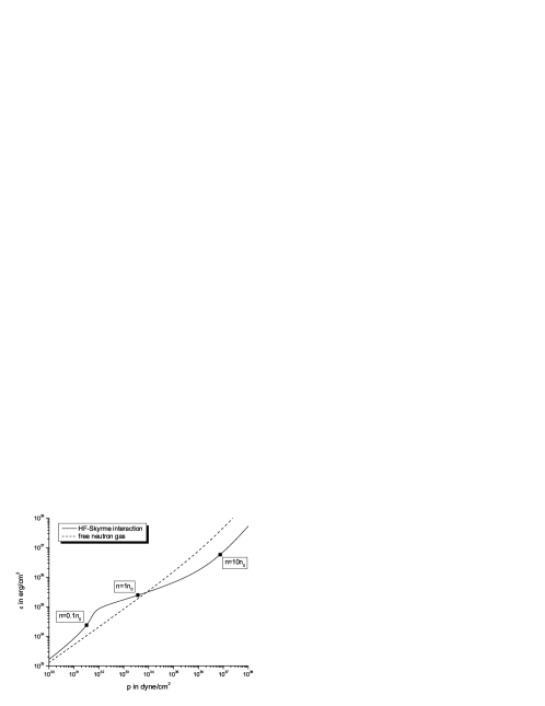
Figure 18: The equation of state for the Skyrme–parameterisation and for a free neutron gas.

Again, we assume pure neutron matter, i.e. we set $N_{p}=0$ and $N_{n}=A$:

$$\frac{E_{HF}}{A}=\frac{3}{5}\frac{k_{n}^{2}}{2m_{n}}+\frac{1}{4}(\frac{1}{6}t_{3}n-t_{0})n.\\$$

With the total energy density $\epsilon(n)$, including the rest mass term $m_{n}\cdot n$,

$$\epsilon(n) = (m_{n}+E_{HF}/A)\cdot n$$ (117)

$$= m_{n}n+\frac{3}{10m_{n}}(3\pi^{2}\hbar^{3})^{2/3}n^{5/3}+\frac{t_{3}}{24}n^{3}-\frac{t_{0}}{4}n^{2},$$ (118)

one can derive $p(n)$ according to the thermodynamic relation:

$$p(n) = n\frac{d}{dn}\epsilon(n)-\epsilon(n)$$ (119)

$$\Longrightarrow p(n) = \frac{2}{10m_{n}}(3\pi^{2}\hbar^{3})^{2/3}n^{5/3}+\frac{t_{3}}{12}n^{3}-\frac{t_{0}}{4}n^{2}.$$ (120)

The resulting equation of state is plotted in Fig. 18, which appears to be very similar to the empirical interaction discussed before.

Figure 19: The mass $M$ as a function of $R$ for the Skyrme–parameterisation. The maximum mass star has a mass of $M=2.438{\ \rm M_{\odot}}$ and a radius of $R=10.98$ km.

Fig. 19 depicts the corresponding mass–radius plot. The maximum mass star has a mass of $M=2.438{\ \rm M_{\odot}}$ and a radius of $R=10.98$ km. These values are only a bit smaller than the ones calculated before for the empirical interaction, also the shape of the curve looks similar. The sharp turnover in the lower left corner of the plot corresponds to a minimal radius of only $R\simeq 8.6$ km and a mass of $M\simeq 0.1{\ \rm M_{\odot}}$.

V.3 Comparing the two models

It is instructive to take a closer look on the two different EoSs considered here, as the results do not differ that much from each other. The two energy densities (eqs. (100) and (118)) are:

• empirical nucleon–nucleon parameterisation:

  $$\frac{\epsilon_{emp}(n)}{n}=m_{n}+\left<E_{0}\right>u^{2/3}+\frac{A}{2}u+\frac{B}{\sigma+1}u^{\sigma}+(2^{2/3}-1)\left<E_{0}\right>\left(u^{2/3}-u\right)+S_{0}u$$ (121)

• Hartree–Fock method and Skyrme parameterisation:

  $$\frac{\epsilon_{HF}(n)}{n}=m_{n}+\frac{3}{10m_{n}}(3\pi^{2}\hbar^{3})^{2/3}n^{2/3}+\frac{1}{4}(\frac{1}{6}t_{3}n-t_{0})n$$ (122)

With $n=u\cdot n_{0}$ and eq. (91) one can rewrite the two equations in the following form:

$$\frac{\epsilon_{emp}(n)}{n} = m_{n}+2^{2/3}\left<E_{0}\right>u^{2/3}+\left(\frac{A}{2}-(2^{2/3}-1)\left<E_{0}\right>+S_{0}\right)u+\frac{B}{\sigma+1}u^{\sigma}$$ (123)

$$\frac{\epsilon_{HF}(n)}{n} = m_{n}+2^{2/3}\left<E_{0}\right>u^{2/3}-\frac{1}{4}t_{0}n_{0}u+\frac{1}{24}t_{3}n_{0}^{2}u^{2}.$$ (124)

By inserting the numbers (115), the energy density exhibits the following parametric form:

$$\frac{\epsilon_{emp}(n)}{n} = (939.6+35.1u^{2/3}-42.1u+21.0u^{2.112}){\ \rm MeV}\stackrel{{\scriptstyle u\gg 1}}{{\longrightarrow}}21.0u^{2.112}{\ \rm MeV}$$ (125)

$$\frac{\epsilon_{HF}(n)}{n} = (939.6+35.1u^{2/3}-41.0u+15.6u^{2}){\ \rm MeV}\stackrel{{\scriptstyle u\gg 1}}{{\longrightarrow}}15.6u^{2}{\ \rm MeV}.$$ (126)

If the energy density follows a power–law as a function of $n$, it is easy to find an explicit equation of state of the form $p(\epsilon)$:

$$\epsilon = c\cdot n^{k}$$

$$p = n\cdot\frac{d\epsilon}{dn}-\epsilon=(k-1)c\cdot n^{k}$$

$$p(\epsilon) = (k-1)\epsilon\quad.$$ (127)

In our case, $k=3.112$ for the empirical interaction and $k=3$ for the Skyrme–parameterisation. One can see, that the first EoS is stiffer than the second. This explains why the masses in the empirical model are bigger as the masses in the Skyrme–parameterisation, the harder EoS can support more mass.

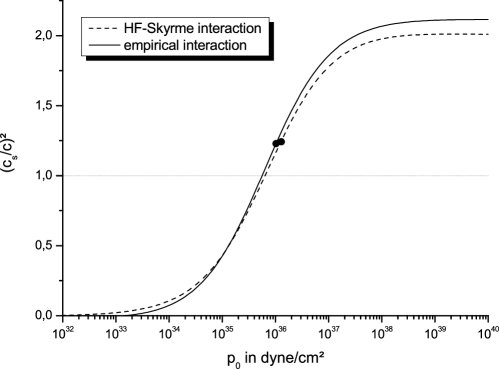
Figure 20: The speed of sound depending on the central pressure for the two different models. The maximum mass stars are marked with a dot.

V.4 Speed of sound and causality

The speed of sound in our neutron star must be less than the speed of light to fulfil relativistic causality. The adiabatic speed of sound is given by $c_{s}=\frac{dp}{d\epsilon}$ in a non–dispersive medium. Hence, we have:

$$1\leq\left(\frac{c_{s}}{c}\right)^{2}=\frac{dp}{d\epsilon}=\frac{dp/dn}{d\epsilon/dn}\quad.$$ (128)

Using eq. (127) one gets:

$$\frac{dp}{d\epsilon}=k-1\leq 1.$$ (129)

Hence, the power coefficient $k$ must be less than or equal two. So both EoSs will become acausal for large $n$. This behaviour is demonstrated in Fig. 20, where the speed of sound is plotted against the central pressure. As one can see, for the maximum mass star the speed of sound $c_{s}/c$ is larger than one for both interactions considered. hence, correction factors have to be added to the interaction, which include (or simulate) relativistic effects (see e.g. Akmal et al. (1998)).

VI Summary and brief overview on present day developments

In chapter II, we discussed the common structure equations for stars as well as the relativistic and non–relativistic equations of state (EoS) for a Fermi gas of electrons and nucleons. We simplified the EoS to a polytropic form and derived semi–analytically the Chandrasekhar mass limit of M = $1.4312\left(2/\eta\right)^{2}{\rm M_{\odot}}$ for white dwarfs. We calculated numerically mass–radius relations for white dwarfs using the relativistic and non–relativistic polytropic approximations. For the relativistic case we find the computed masses to be constant and in very good agreement with the Chandrasekhar mass limit. The numerical results were also checked by the analytical results for white dwarf radii.

We introduced a numerical method to calculate the EoS of a free gas of particles for the general case, i.e. without using the polytropic approximation, and computed the corresponding masses and radii for white dwarfs. In this case, the calculated masses became larger with increasing central pressures up to a maximum mass of around 1.4 ${\rm M_{\odot}}$. For high pressures, the masses stayed constant at the maximum value showing that the EoS turned into a relativistic polytrope.

We calculated the mass–radius relations without as well as with corrections from general relativity. The mass curve showed an increasing mass for larger central pressures up to $p_{0}\sim 10^{28}{\rm dyne/cm^{2}}$ reaching a maximum mass of about 1.40 ${\rm M_{\odot}}$ without and one of 1.39 ${\rm M_{\odot}}$ with relativistic corrections. The slightly reduced maximum mass in the latter case was in accord with the fact that general relativity corrections strengthen the gravitational force.

We discussed also that white dwarfs and neutron stars are stable against radial oscillations for masses smaller than the maximum mass but unstable beyond the mass peak.

In chapter III, we looked at pure neutron stars using an EoS of a free Fermi gas of neutrons. We computed the exact equation of state by a root finding routine. The maximum mass for such a neutron star was found to be $M=0.712$ M_⊙ with a radius of $R=9.14$ km. Then, we included protons and electrons in $\beta$–equilibrium to the composition of neutron star matter. The maximum mass of the corresponding neutron star changed slightly to $M=0.699{\ \rm M_{\odot}}$ and the radius to $R=9.24$ km.

Next, we focused on the impact of nuclear interactions on the properties of pure neutron stars. We analysed two different types of interaction, an empirical interaction and the Hartree–Fock method applied to a Skyrme–parameterisation. As the two resulting EoSs were very close to each other, the results for the mass and radius curves were very similar, but quite different to the cases of free Fermi gases considered before. The maximum masses of neutron stars reach now values of $M=2.4M_{\odot}$ and $M=2.8M_{\odot}$, respectively, which are up to four times larger than for the free cases. The corresponding radii increase to $R=11$ to 12 km, respectively. The repulsion between nucleons stiffens the EoS, increases the pressure at fixed energy density, and enables to stabilise more massive neutron stars compared to the free Fermi gas case. Caveats of the simple nuclear interaction models used were exhibited, as the neglect of relativistic effects and the EoSs becoming acausal for large central pressures.

We close this section with a brief discussion of present day developments in the field of compact stars: astrophysical data, the EoS of dense matter and its impact on the global properties of compact stars (for a recent general introduction on latest developments in the field we refer to Lattimer and Prakash (2004)).

More than 1500 pulsars, rotating neutron stars with pulsed radio emission, are known today. About seven thermally emitting isolated neutron stars have been observed by the Hubble Space Telescope (HST), by the x–ray satellites Chandra and XMM–Newton and by ground based optical telescopes as the European Southern Observatory ESO. For the closed and best studied one, RX J1856.5-3754, the measured spectra can be well described by a Planck curve Drake et al. (2002). As the outermost layer of a neutron star is the atmosphere up to a density of $10^{4}$ gm/cm³ consists of atoms, their presence should show up in the spectra. However, there is a lack of any atomic spectral line in the spectra which is not understood at present Burwitz et al. (2003). For three selected rotating neutron stars (pulsars), nicknamed the Three Musketeers, one is even able to make phase resolved studies of the spectra, which allows to determine that there are hot spots on the surface of the neutron star De Luca et al. (2005).

The high–density EoS for neutron stars and the appearance of exotic matter has been studied in modern relativistic field–theoretical models Glendenning (2000). In particular, hyperons will appear around twice normal nuclear matter density (see e.g. Schaffner-Bielich (2004) and references therein). The possibility of Bose condensation of kaons in dense, cold matter has been investigated also Li et al. (1997). Last but not least, the phase transition to strange quark matter, quark matter with strange quarks, will appear in the high–density limit Weber (2005); Schaffner-Bielich (2005). If the phase transition of these exotic forms of matter is strongly first order, a new class of compact stars emerges as a new stable solution of the TOV equations. While the existence of this third family of compact stars besides white dwarfs and neutron stars was known earlier Gerlach (1968); Haensel and Prószyński (1980); Kämpfer (1981), the solution was rediscovered in modern models for the EoS and a Gibbs phase transition only recently Glendenning and Kettner (2000); Schertler et al. (2000); Schaffner-Bielich et al. (2002); Fraga et al. (2001). The topic of the third family of compact stars was a subject for another undergraduate student project of Jean Macher and one of the authors Macher and Schaffner-Bielich (2005). The study of dense quark matter, as possibly present in the core of neutron stars, has been the object of intense investigation during the last few years due to the rediscovery of the phenomenon of colour superconductivity. Here, two colour charged quarks form a (colour) superconducting state and change the properties of quark matter (for reviews see e.g. Rajagopal and Wilczek (2000); Alford (2004); Rischke (2004)). Neutron stars with colour superconducting quark matter have been calculated by many authors in the last couple of years, see Alford and Reddy (2003); Lugones and Horvath (2003); Baldo et al. (2003); Banik and Bandyopadhyay (2003); Blaschke et al. (2003); Shovkovy et al. (2003); Grigorian et al. (2004); Rüster and Rischke (2004); Buballa et al. (2004); Drago et al. (2004); Alford et al. (2004). The physics of strange quark matter in compact stars and its possible signals are reviewed most recently also in Weber (2005); Schaffner-Bielich (2005).

The physics of neutron star has also impacts not only on pulsars but also in other active research fields of astrophysics. For example, in x–ray binaries a neutron star accretes matter from his companion, which is an ordinary star or a white dwarf. When the matter falls onto the neutron star, x–ray bursts occur. Redshifted spectral lines have been measured from such x–ray binaries, which allow to constrain the compactness and by that the EoS of neutron stars Cottam et al. (2002). Core collapse supernovae form a hot proto–neutron star first which cools subsequently and emits a neutrino wind. That neutrino wind influences the production of heavy elements in the supernova material in the so called r–process nucleosynthesis (see e.g. Langanke and Martinez-Pinedo (2003) and references therein). Neutron stars can collide with a corresponding emission of gravitational waves, which will be measured by gravitational wave detectors in the near future, and gamma–rays, being considered a prime candidate for gamma-ray bursts and another site for r–process nucleosynthesis. The dynamics of the collision depends on the underlying EoS of neutron stars Oechslin et al. (2004)! In the future, the square kilometre array (SKA) will measure more than 10.000 pulsars, with expected 100 binary systems with a neutron stars Kramer (2003), so the prospects are bright for learning more about the physics of neutron stars!

References

- Silbar and Reddy (2004) R. R. Silbar and S. Reddy, Am. J. Phys. 72, 892 (2004), eprint nucl-th/0309041.
- Shapiro and Teukolsky (1983) S. L. Shapiro and S. A. Teukolsky, Black Holes, White Dwarfs, and Neutron Stars: The Physics of Compact Objects (John Wiley & Sons, New York, 1983).
- Herrera and Barreto (2004) L. Herrera and W. Barreto, Gen. Rel. Grav. 36, 127 (2004), eprint gr-qc/0309052.
- Chandrasekhar (1931) S. Chandrasekhar, Astrophys. J. 74, 81 (1931).
- Weinberg (1972) S. Weinberg, Gravitation and Cosmology: Principles and Applications of the General Theory of Relativity (John Wiley and Sons, New York, 1972).
- Landau (1932) L. D. Landau, Physik. Zeits. Sowjetunion 1, 285 (1932).
- Eidelman et al. (2004) S. Eidelman et al., Phys. Lett. B 592, 1 (2004), URL http://pdg.lbl.gov.
- Weber (1999) F. Weber, Pulsars as Astrophysical Laboratories for Nuclear and Particle Physics (Institute of Physics, Bristol, 1999).
- Hanauske (2004) M. Hanauske, Ph.D. thesis, Goethe Universität, Frankfurt am Main, Germany (2004), URL http://www.th.physik.uni-frankfurt.de/~hanauske/diss_hanauske.pdf.
- Herrera and Santos (1997) L. Herrera and N. O. Santos, Phys. Rep. 286, 53 (1997).
- Harrison (1965) B. K. Harrison, Phys. Rep. 137, 1644 (1965).
- Harrison et al. (1965) B. K. Harrison, K. S. Thorne, M. Wakano, and J. A. Wheeler, Gravitation Theory and Gravitational Collapse (The Unversity of Chicago Press, Chicago, 1965).
- Glendenning (2000) N. K. Glendenning, Compact Stars — Nuclear Physics, Particle Physics, and General Relativity (Springer, New York, 2000), 2nd ed.
- Gerlach (1968) U. H. Gerlach, Phys. Rev. 172, 1325 (1968).
- Glendenning and Kettner (2000) N. K. Glendenning and C. Kettner, Astron. Astrophys. 353, L9 (2000), eprint astro-ph/9807155.
- Schertler et al. (2000) K. Schertler, C. Greiner, J. Schaffner-Bielich, and M. H. Thoma, Nucl. Phys. A677, 463 (2000), eprint astro-ph/0001467.
- Oppenheimer and Volkoff (1939) J. R. Oppenheimer and G. M. Volkoff, Phys. Rev. 55, 374 (1939).
- Haensel et al. (2002) P. Haensel, J. L. Zdunik, and F. Douchin, Astron. Astrophys. 385, 301 (2002).
- Prakash et al. (1988) M. Prakash, T. L. Ainsworth, and J. M. Lattimer, Phys. Rev. Lett. 61, 2518 (1988).
- Baym et al. (1971) G. Baym, C. Pethick, and P. Sutherland, Astrophys. J. 170, 299 (1971).
- Haensel (2001) P. Haensel, in Physics of Neutron Star Interiors, edited by D. Blaschke, N. K. Glendenning, and A. Sedrakian (Springer, Heidelberg, 2001), vol. 578 of Lecture Notes in Physics, pp. 127–174.
- Greiner (2004) C. Greiner, Lecture notes of ”Quantum Mechanics II” (2004).
- Ring and Schuck (2004) P. Ring and P. Schuck, The Nuclear Many-Body Problem (Springer, Berlin, 2004).
- Akmal et al. (1998) A. Akmal, V. R. Pandharipande, and D. G. Ravenhall, Phys. Rev. C 58, 1804 (1998).
- Lattimer and Prakash (2004) J. M. Lattimer and M. Prakash, Science 304, 536 (2004).
- Drake et al. (2002) J. J. Drake et al., Astrophys. J. 572, 996 (2002).
- Burwitz et al. (2003) V. Burwitz, F. Haberl, R. Neuhäuser, P. Predehl, J. Trümper, and V. E. Zavlin, Astron. Astrophys. 399, 1109 (2003), eprint astro-ph/0211536.
- De Luca et al. (2005) A. De Luca, P. A. Caraveo, S. Mereghetti, M. Negroni, and G. F. Bignami, Astrophys. J. 623, 1051 (2005).
- Schaffner-Bielich (2004) J. Schaffner-Bielich, astro-ph/0402597 (2004).
- Li et al. (1997) G.-Q. Li, C. H. Lee, and G. E. Brown, Nucl. Phys. A625, 372 (1997), eprint nucl-th/9706057.
- Weber (2005) F. Weber, Prog. Part. Nucl. Phys. 54, 193 (2005), eprint astro-ph/0407155.
- Schaffner-Bielich (2005) J. Schaffner-Bielich, J. Phys. G 31, S651 (2005), eprint astro-ph/0412215.
- Haensel and Prószyński (1980) P. Haensel and M. Prószyński, Phys. Lett. B96, 233 (1980).
- Kämpfer (1981) B. Kämpfer, J. Phys. A 14, L471 (1981).
- Schaffner-Bielich et al. (2002) J. Schaffner-Bielich, M. Hanauske, H. Stöcker, and W. Greiner, Phys. Rev. Lett. 89, 171101 (2002), eprint astro-ph/0005490.
- Fraga et al. (2001) E. S. Fraga, R. D. Pisarski, and J. Schaffner-Bielich, Phys. Rev. D 63, 121702(R) (2001), eprint hep-ph/0101143.
- Macher and Schaffner-Bielich (2005) J. Macher and J. Schaffner-Bielich, Eur. J. Phys. 26, 341 (2005), eprint astro-ph/0411295.
- Rajagopal and Wilczek (2000) K. Rajagopal and F. Wilczek, hep-ph/0011333 (2000).
- Alford (2004) M. Alford, Prog. Theor. Phys. Suppl. 153, 1 (2004), eprint nucl-th/0312007.
- Rischke (2004) D. H. Rischke, Prog. Part. Nucl. Phys. 52, 197 (2004).
- Alford and Reddy (2003) M. Alford and S. Reddy, Phys. Rev. D 67, 074024 (2003), eprint nucl-th/0211046.
- Lugones and Horvath (2003) G. Lugones and J. E. Horvath, Astron. Astrophys. 403, 173 (2003), eprint astro-ph/0211638.
- Baldo et al. (2003) M. Baldo, M. Buballa, F. Burgio, F. Neumann, M. Oertel, and H. J. Schulze, Phys. Lett. B 562, 153 (2003), eprint nucl-th/0212096.
- Banik and Bandyopadhyay (2003) S. Banik and D. Bandyopadhyay, Phys. Rev. D 67, 123003 (2003), eprint astro-ph/0212340.
- Blaschke et al. (2003) D. Blaschke, H. Grigorian, D. N. Aguilera, S. Yasui, and H. Toki, AIP Conf. Proc. 660, 209 (2003), eprint hep-ph/0301087.
- Shovkovy et al. (2003) I. Shovkovy, M. Hanauske, and M. Huang, Phys. Rev. D 67, 103004 (2003), eprint hep-ph/0303027.
- Grigorian et al. (2004) H. Grigorian, D. Blaschke, and D. N. Aguilera, Phys. Rev. C 69, 065802 (2004), eprint astro-ph/0303518.
- Rüster and Rischke (2004) S. B. Rüster and D. H. Rischke, Phys. Rev. D 69, 045011 (2004), eprint nucl-th/0309022.
- Buballa et al. (2004) M. Buballa, F. Neumann, M. Oertel, and I. Shovkovy, Phys. Lett. B 595, 36 (2004), eprint nucl-th/0312078.
- Drago et al. (2004) A. Drago, A. Lavagno, and G. Pagliara, Phys. Rev. D 69, 057505 (2004).
- Alford et al. (2004) M. Alford, M. Braby, M. Paris, and S. Reddy, nucl-th/0411016 (2004).
- Cottam et al. (2002) J. Cottam, F. Paerels, and M. Mendez, Nature 420, 51 (2002), eprint astro-ph/0211126.
- Langanke and Martinez-Pinedo (2003) K. Langanke and G. Martinez-Pinedo, Rev. Mod. Phys. 75, 819 (2003), eprint nucl-th/0203071.
- Oechslin et al. (2004) R. Oechslin, K. Uryū, G. Poghosyan, and F. K. Thielemann, Mon. Not. R. Astron. Soc. 349, 1469 (2004).
- Kramer (2003) M. Kramer, astro-ph/0306456 (2003).