An HLLC Riemann Solver for Relativistic Flows: I. Hydrodynamics

Abstract

We present an extension of the HLLC approximate Riemann solver by Toro, Spruce and Speares to the relativistic equations of fluid dynamics. The solver retains the simplicity of the original two-wave formulation proposed by Harten, Lax and van Leer (HLL) but it restores the missing contact wave in the solution of the Riemann problem. The resulting numerical scheme is computationally efficient, robust and positively conservative. The performance of the new solver is evaluated through numerical testing in one and two dimensions.

1 Introduction

High energy astrophysical phenomena involve, in many cases, relativistic flows, typical examples are superluminal motion of relativistic jets in extragalactic radio sources, accretion flows around massive compact objects, pulsar winds and Gamma Ray Bursts. The modeling of such phenomena has prompted the search for efficient and accurate numerical formulations of the special relativistic fluid equations (for an excellent review see Martí & Müller, 2003). There is now a strong consensus that the so-called “high-resolution shock-capturing” schemes provide the necessary tools in developing stable and robust relativistic fluid dynamical codes. One of the fundamental ingredients of such schemes is the exact or approximate solution to the Riemann problem.

The solution to the Riemann problem in relativistic hydrodynamics (RHD henceforth) has been extensively studied in literature, and an exact solution can be found within high degree of accuracy by iterative techniques, see Martí & Müller (1994), Pons et al. (2000), Rezzolla et al. (2003) and references therein. One of the major differences with the classical counterpart is the velocity coupling introduced by the Lorentz factor and the coupling of the latter with the specific enthalpy. This considerably adds to the computational cost, making the use of an exact solver code prohibitive in a multidimensional Godunov-type code.

From this perspective, approximate solvers based on alternative strategies have been devised: local linearization (Eulderink & Mellema, 1995; Falle & Komissarov, 1996), two-shock approximation (Balsara, 1994; Dai & Woodward, 1997; Mignone et al., 2005), flux-splitting methods (Donat et al., 1998), and so forth, see Martí & Müller (2003) for a comprehensive review. Most of these solvers, however, rely on rather expensive characteristic decompositions of the Jacobian matrix or involve iterative techniques to solve highly nonlinear equations. Although they usually attain better resolution at discontinuities, some of these methods may produce unphysical states with negative densities or pressures, as it has been shown by Einfeldt et al. (1991) for linearized Riemann solvers in the context of classical hydrodynamics.

The HLL method devised by Harten et al. (1983) for classical gasdynamics belongs to a different class of approximate Riemann solvers and has gained increasing popularity among researchers in the last decade. It has been implemented in the context of the relativistic fluid equations by Schneider et al. (1993) and Duncan & Hughes (1994). The HLL approach does not require a full characteristic decomposition of the equations and is straightforward to implement in a Godunov-type code. Besides the computational efficiency, this class of solvers has the attractive feature of being positively conservative in the sense that preserve initially positive densities, energy and pressures.

The HLL formulation, however, lacks the ability to resolve isolated contact discontinuity and for this reason has a more diffusive character than other more sophisticated algorithms. To compensate for this, Toro et al. (1994) developed an extension of the HLL solver for the Euler equations introducing a two-state HLL-type solver called HLLC (where “C” stands for contact) that improves the treatment of the contact discontinuity, see also Batten et al. (1997). Recently this approach has been generalized to the magnetohydrodynamic equations (Gurski, 2004; Li, 2005).

In the present work, we extend this approach to the relativistic equation of fluid dynamics. The paper is structured as follows: in §2 the relevant equations are given, in §3 we describe the new approximate Riemann solver and in §4 we asses the strength of the new method with one and two dimensional tests.

2 The RHD Equations

The motion of an ideal relativistic fluid is governed by conservation of mass, momentum and energy. The pertaining equations are cast as a hyperbolic system of conservation laws (Landau & Lifshitz, 1959) which, in two dimensions, reads

$$\frac{\partial\mn@boldsymbol{U}}{\partial t}+\frac{\partial\mn@boldsymbol{F}^{x}(\mn@boldsymbol{U})}{\partial x}+\frac{\partial\mn@boldsymbol{F}^{y}(\mn@boldsymbol{U})}{\partial y}=0\,,$$ (1)

where $\mn@boldsymbol{U}=(D,m_{x},m_{y},E)$ is the unknown vector of conservative variables, whereas $\mn@boldsymbol{F}^{x}$ and $\mn@boldsymbol{F}^{y}$ are, respectively, the fluxes along the $x$ and $y$ directions:

$$\mn@boldsymbol{F}^{x}(\mn@boldsymbol{U})=\left(\begin{array}[]{c}Dv_{x}\\ \vskip 6.0pt plus 2.0pt minus 2.0pt\cr m_{x}v_{x}+p\\ \vskip 6.0pt plus 2.0pt minus 2.0pt\cr m_{y}v_{x}\\ \vskip 6.0pt plus 2.0pt minus 2.0pt\cr m_{x}\\ \vskip 6.0pt plus 2.0pt minus 2.0pt\cr\end{array}\right)\,,\quad\mn@boldsymbol{F}^{y}(\mn@boldsymbol{U})=\left(\begin{array}[]{c}Dv_{y}\\ \vskip 6.0pt plus 2.0pt minus 2.0pt\cr m_{x}v_{y}\\ \vskip 6.0pt plus 2.0pt minus 2.0pt\cr m_{y}v_{y}+p\\ \vskip 6.0pt plus 2.0pt minus 2.0pt\cr m_{y}\\ \vskip 6.0pt plus 2.0pt minus 2.0pt\cr\end{array}\right)\,.$$ (2)

Generalization to three dimensions is straightforward.

In equations (2), $p$ is the thermal pressure, whereas $D$, $\mn@boldsymbol{m}\equiv(m_{x},m_{y})$ and $E$ are, respectively, the mass, momentum and energy densities relative to the lab frame, where the fluid has velocity $\mn@boldsymbol{v}\equiv(v_{x},v_{y})$. Units are conveniently normalized so that the speed of light is $c=1$.

The relation between conserved variables $\mn@boldsymbol{U}$ and physical quantities $\mn@boldsymbol{V}=\big{(}\rho,v_{x},v_{y},p\big{)}$ is

$$D=\gamma\rho\,,\quad\mn@boldsymbol{m}=Dh\gamma\mn@boldsymbol{v}\,,\quad E=Dh\gamma-p\,,$$ (3)

where $\rho$ is the proper rest mass density, $\gamma=(1-\mn@boldsymbol{v}\cdot\mn@boldsymbol{v})^{-\frac{1}{2}}$ is the Lorentz factor and $h$ is the specific enthalpy. Proper closure is provided by specifying an equation of state in the form $h=h(p,\rho)$.

For an ideal gas, the enthalpy has the form $\rho h=\rho+p\Gamma/(\Gamma-1)$ and the sound speed is defined by

$$c_{s}=\sqrt{\frac{\Gamma p}{\rho h}}\,.$$ (4)

with $\Gamma$ being the (constant) specific heat ratio. By letting $p/\rho\to\infty$, we see that the square of the sound speed has the limiting value $c_{s}^{2}\to\Gamma-1$. Since it can be shown (Taub, 1948; Anile, 1989; Mignone et al., 2005) that the specific heat ratio $\Gamma$ cannot exceed $2$, one always has $c_{s}^{2}<1$. This is an important result for the positivity of the HLL and HLLC schemes and will be used in a later section.

Equation (3) gives $\mn@boldsymbol{U}$ in terms of the primitive state vector $\mn@boldsymbol{V}$. The inverse relation involves the solution of a nonlinear equation for the pressure $p$:

$$E+p=D\gamma+\frac{\Gamma}{\Gamma-1}p\gamma^{2}$$ (5)

where $\gamma=\big{[}1-|\mn@boldsymbol{m}|^{2}/(E+p)^{2}\big{]}^{-\frac{1}{2}}$. Equation (5) can be solved by any standard root finding algorithm.

2.1 The Riemann Problem in RHD

Consider a conservative discretization of (1) along the x-direction:

$$\frac{\bar{\mn@boldsymbol{U}}^{n+1}_{i}-\bar{\mn@boldsymbol{U}}^{n}_{i}}{\Delta t^{n}}=\frac{\mn@boldsymbol{f}_{i+\frac{1}{2}}-\mn@boldsymbol{f}_{i-\frac{1}{2}}}{\Delta x_{i}}\,.$$ (6)

The numerical flux functions $\mn@boldsymbol{f}_{i+\frac{1}{2}}$ follow from the solution of Riemann problems with initial data:

$$\mn@boldsymbol{U}(x,0)=\left\{\begin{array}[]{ccc}\mn@boldsymbol{U}_{L,i+\frac{1}{2}}&\quad\textrm{if}&x<x_{i+\frac{1}{2}}\,,\\ \vskip 6.0pt plus 2.0pt minus 2.0pt\cr\mn@boldsymbol{U}_{R,i+\frac{1}{2}}&\quad\textrm{if}&x>x_{i+\frac{1}{2}}\,,\\ \vskip 6.0pt plus 2.0pt minus 2.0pt\cr\end{array}\right.$$ (7)

where $\mn@boldsymbol{U}_{L,i+\frac{1}{2}}$ and $\mn@boldsymbol{U}_{R,i+\frac{1}{2}}$ are the left and right edge values at zone interfaces.

Figure 1: Graphical representation of the Riemann fan in the $x-t$ plane. The two initial states $\mn@boldsymbol{U}_{L}$ and $\mn@boldsymbol{U}_{R}$ decay into two nonlinear waves (with speeds $\lambda_{L}$ and $\lambda_{R}$) and a linear contact wave with velocity $\lambda^{*}$. The resulting wave pattern divides the $x-t$ plane into four regions each defining a constant state: $\mn@boldsymbol{U}_{L}$, $\mn@boldsymbol{U}^{*}_{L}$, $\mn@boldsymbol{U}^{*}_{R}$ and $\mn@boldsymbol{U}_{R}$.

The solution of the Riemann problem for the special relativistic fluid equations has been investigated by Martí & Müller (1994), Pons et al. (2000), Rezzolla et al. (2003). It consists of a self-similar three-wave pattern generated by the decay of the initial discontinuity (7). The resulting Riemann fan (Fig. 1) is bounded by two nonlinear waves (representing either shocks or rarefactions) separated by a contact discontinuity moving at the fluid velocity. Across the contact discontinuity, pressure and normal velocity are continuous whereas density and tangential velocities experience jumps. The same holds also in the non-relativistic limit. Contrary to the Newtonian counterpart, however, all variables are discontinuous across a shock wave or change smoothly through a rarefaction fan (Pons et al., 2000). This is a consequence of the velocity coupling introduced by the Lorentz factor $\gamma$ and by the coupling of the latter with the specific enthalpy $h$.

The resulting wave pattern can be solved to a high degree of precision by iterative techniques and has been implemented for the first time in the one-dimensional Godunov-type code by Martí & Müller (1996). Nevertheless, when tangential velocities are included, the computational effort increases considerably, and the use of an exact solver in a multidimensional Godunov-type code can become prohibitive.

Here we consider a different approach, based on the original prescription given by Harten et al. (1983) (HLL) for the classical Euler equations and subsequently extended by Toro et al. (1994) (HLLC). Both the HLL and HLLC formulations do not require a field by field decomposition of the relativistic equations, a feature which makes them particularly attractive, specially in multi-dimensional applications.

3 The HLL Framework

Harten, Lax and van Leer (Harten et al., 1983) proposed an approximate solution to the Riemann problem where the two states bounded by the two acoustic waves are averaged into a single constant state. In other words, the solution to the Riemann problem on the $x/t=0$ axis consists of the three possible constant states:

$$\mn@boldsymbol{U}(0,t)=\left\{\begin{array}[]{cll}\mn@boldsymbol{U}_{L}&\;\textrm{if}&\lambda_{L}\geq 0\,,\\ \vskip 6.0pt plus 2.0pt minus 2.0pt\cr\mn@boldsymbol{U}^{hll}&\;\textrm{if}&\lambda_{L}\leq 0\leq\lambda_{R}\,,\\ \vskip 6.0pt plus 2.0pt minus 2.0pt\cr\mn@boldsymbol{U}_{R}&\;\textrm{if}&\lambda_{R}\leq 0\,,\\ \vskip 6.0pt plus 2.0pt minus 2.0pt\cr\end{array}\right.$$ (8)

where we dropped, for simplicity, the half integer notation $i+\frac{1}{2}$. Harten et al. (1983) noted that the single state $\mn@boldsymbol{U}^{hll}$ could be constructed from an a priori estimate of the fastest and slowest signal velocities $\lambda_{L}$ and $\lambda_{R}$:

$$\mn@boldsymbol{U}^{hll}=\frac{\lambda_{R}\mn@boldsymbol{U}_{R}-\lambda_{L}\mn@boldsymbol{U}_{L}+\mn@boldsymbol{F}_{L}-\mn@boldsymbol{F}_{R}}{\lambda_{R}-\lambda_{L}}\,,$$ (9)

where $\mn@boldsymbol{F}_{L}=\mn@boldsymbol{F}^{x}(\mn@boldsymbol{U}_{L})$, $\mn@boldsymbol{F}_{R}=\mn@boldsymbol{F}^{x}(\mn@boldsymbol{U}_{R})$. Notice that equation (9) represents the integral average of the solution of the Riemann problem over the wave fan (Toro, 1997).

The corresponding interface numerical flux is defined as:

$$\mn@boldsymbol{f}=\left\{\begin{array}[]{cll}\mn@boldsymbol{F}_{L}&\;\textrm{if}&\lambda_{L}\geq 0\,,\\ \vskip 6.0pt plus 2.0pt minus 2.0pt\cr\mn@boldsymbol{F}^{hll}&\;\textrm{if}&\lambda_{L}\leq 0\leq\lambda_{R}\,,\\ \vskip 6.0pt plus 2.0pt minus 2.0pt\cr\mn@boldsymbol{F}_{R}&\;\textrm{if}&\lambda_{R}\leq 0\,,\\ \vskip 6.0pt plus 2.0pt minus 2.0pt\cr\end{array}\right.$$ (10)

where

$$\mn@boldsymbol{F}^{hll}=\frac{\lambda_{R}\mn@boldsymbol{F}_{L}-\lambda_{L}\mn@boldsymbol{F}_{R}+\lambda_{R}\lambda_{L}(\mn@boldsymbol{U}_{R}-\mn@boldsymbol{U}_{L})}{\lambda_{R}-\lambda_{L}}\,.$$ (11)

Thus, given a wave speed estimate for the fastest and slowest speeds $\lambda_{R}$ and $\lambda_{L}$ (see §3.1.1), an approximate solution to the Riemann problem can be constructed and the intercell numerical fluxes for the conservative update (6) are computed using (10).

This approach has been applied for the first time to the one-dimensional relativistic equations by Schneider et al. (1993) and later by Duncan & Hughes (1994) for the multidimensional case.

Although the HLL prescription is computationally inexpensive and straightforward to implement, a major drawback is its inability to resolve contact or tangential waves. On the contrary the HLLC scheme, originally introduced by Toro et al. (1994) in the context of the Euler equations of classical gasdynamics, does not suffer from this loss. In the next section we generalize this approach to the equations of relativistic hydrodynamics.

3.1 HLLC Solver

The HLLC scheme restores the full wave structure inside the Riemann fan by replacing the single averaged state defined by (9) with two approximate states, $\mn@boldsymbol{U}^{*}_{L}$ and $\mn@boldsymbol{U}^{*}_{R}$. These two states are separated by a middle contact wave which is assumed to have constant speed $\lambda^{*}$, so that the full solution to the Riemann problem now reads

$$\mn@boldsymbol{U}(0,t)=\left\{\begin{array}[]{ccc}\mn@boldsymbol{U}_{L}&\quad\textrm{if}&\;\lambda_{L}\geq 0\,,\\ \vskip 6.0pt plus 2.0pt minus 2.0pt\cr\mn@boldsymbol{U}^{*}_{L}&\quad\textrm{if}&\;\lambda_{L}\leq 0\leq\lambda^{*}\,,\\ \vskip 6.0pt plus 2.0pt minus 2.0pt\cr\mn@boldsymbol{U}^{*}_{R}&\quad\textrm{if}&\;\lambda^{*}\leq 0\leq\lambda_{R}\,,\\ \vskip 6.0pt plus 2.0pt minus 2.0pt\cr\mn@boldsymbol{U}_{R}&\quad\textrm{if}&\;\lambda_{R}\leq 0\,,\\ \vskip 6.0pt plus 2.0pt minus 2.0pt\cr\end{array}\right.$$ (12)

and the corresponding intercell numerical fluxes are:

$$\mn@boldsymbol{f}=\left\{\begin{array}[]{ccc}\mn@boldsymbol{F}_{L}&\quad\textrm{if}&\;\lambda_{L}\geq 0\,,\\ \vskip 6.0pt plus 2.0pt minus 2.0pt\cr\mn@boldsymbol{F}^{*}_{L}&\quad\textrm{if}&\;\lambda_{L}\leq 0\leq\lambda^{*}\,,\\ \vskip 6.0pt plus 2.0pt minus 2.0pt\cr\mn@boldsymbol{F}^{*}_{R}&\quad\textrm{if}&\;\lambda^{*}\leq 0\leq\lambda_{R}\,,\\ \vskip 6.0pt plus 2.0pt minus 2.0pt\cr\mn@boldsymbol{F}_{R}&\quad\textrm{if}&\;\lambda_{R}\leq 0\,.\\ \vskip 6.0pt plus 2.0pt minus 2.0pt\cr\end{array}\right.$$ (13)

The intermediate state fluxes $\mn@boldsymbol{F}^{*}_{L}$ and $\mn@boldsymbol{F}^{*}_{R}$ may be expressed in terms of $\mn@boldsymbol{U}^{*}_{L}$ and $\mn@boldsymbol{U}^{*}_{R}$ from the Rankine-Hugoniot jump conditions:

$$\lambda\left(\mn@boldsymbol{U}^{*}-\mn@boldsymbol{U}\right)=\mn@boldsymbol{F}^{*}-\mn@boldsymbol{F}\,,$$ (14)

where here and throughout the following, quantities without a suffix $L$ or $R$ refer indifferently to the left ($L$) or right ($R$) states. Notice that, in general, $\mn@boldsymbol{F}=\mn@boldsymbol{F}^{x}(\mn@boldsymbol{U})$ but $\mn@boldsymbol{F}^{*}\neq\mn@boldsymbol{F}^{x}(\mn@boldsymbol{U}^{*})$.

We remind the reader that the HLL and HLLC solvers differ in the representation of the intermediate states. In the case of supersonic flows ($\lambda_{L}>0$ or $\lambda_{R}<0$), in fact, the two solvers become equivalent. The same result also holds for an exact Riemann solver.

If $\lambda_{L}$ and $\lambda_{R}$ are given (see §3.1.1), equation (14) represent a system of $2n$ equations (where $n$ is the number of components of $\mn@boldsymbol{U}$) for the $4n+1$ unknowns $\mn@boldsymbol{U}^{*}_{L}$, $\mn@boldsymbol{U}^{*}_{R}$, $\mn@boldsymbol{F}^{*}_{L}$, $\mn@boldsymbol{F}^{*}_{R}$ and $\lambda^{*}$. Three additional constraints come from the requirements that both pressure and normal velocity be continuous across the contact wave (i.e. $v^{*}_{x,R}=v^{*}_{x,L}$, $p^{*}_{R}=p^{*}_{L}$) and that $\lambda^{*}=v_{x,L}^{*}=v_{x,R}^{*}$. This, however, yields a total of only $2n+3$ equations, still not sufficient to solve the system. In order to reduce the number of unknowns and have a well-posed problem, further assumptions have to be made on the form of the fluxes $\mn@boldsymbol{F}^{*}$. Here we assume that the two-dimensional fluxes can be written as

$$\mn@boldsymbol{F}^{*}=\left(\begin{array}[]{c}D^{*}v_{x}^{*}\\ \vskip 6.0pt plus 2.0pt minus 2.0pt\cr m_{x}^{*}v_{x}^{*}+p^{*}\\ \vskip 6.0pt plus 2.0pt minus 2.0pt\cr m_{y}^{*}v_{x}^{*}\\ \vskip 6.0pt plus 2.0pt minus 2.0pt\cr m_{x}^{*}\end{array}\right)\,.$$ (15)

In such a way, both $\mn@boldsymbol{U}^{*}$ and $\mn@boldsymbol{F}^{*}$ are expressed in terms of the five unknowns $D^{*}$, $v_{x}^{*}$, $m_{y}^{*}$, $E^{*}$ and $p^{*}$. The normal components of momentum in the star region, $m^{*}_{x,L}$ and $m^{*}_{x,R}$, are not independent variables since, for consistency, we require that $m_{x}^{*}=(E^{*}+p^{*})v_{x}^{*}$. In the classical case, this assumption becomes equivalent to $m^{*}_{x}=\rho^{*}\lambda^{*}$. This yields a total of $11$ equations in $11$ unknowns.

Writing explicitly equation (14) for the left or the right state yields

$$\begin{array}[]{lcl}D^{*}(\lambda-\lambda^{*})&=&D(\lambda-v_{x})\,,\\ \vskip 6.0pt plus 2.0pt minus 2.0pt\cr m_{x}^{*}(\lambda-\lambda^{*})&=&m_{x}(\lambda-v_{x})+p^{*}-p\,,\\ \vskip 6.0pt plus 2.0pt minus 2.0pt\cr m_{y}^{*}(\lambda-\lambda^{*})&=&m_{y}(\lambda-v_{x})\,,\\ \vskip 6.0pt plus 2.0pt minus 2.0pt\cr E^{*}(\lambda-\lambda^{*})&=&E(\lambda-v_{x})+p^{*}\lambda^{*}-pv_{x}\,.\end{array}$$ (16)

If one combines the last of (16) together with the second one, the following expression giving $\lambda^{*}$ in terms of $p^{*}$ may be obtained:

$$(A-\lambda p^{*})v_{x}^{*}=B+p^{*}\,,$$ (17)

where $A=\lambda E-m_{x}$, $B=m_{x}(\lambda-v_{x})-p$.

By imposing $p^{*}_{x,L}=p^{*}_{x,R}$ across the contact discontinuity we find the following quadratic equation for $\lambda^{*}$:

$$F_{E}^{hll}\left(\lambda^{*}\right)^{2}-(E^{hll}+F_{m_{x}}^{hll})\lambda^{*}+m_{x}^{hll}=0\,.$$ (18)

In equation (18), $F_{E}^{hll}$ and $F_{m_{x}}^{hll}$ are the energy and momentum components of the HLL flux given by equation (11), whereas $E^{hll}$ and $m_{x}^{hll}$ are the energy and normal momentum components of the HLL state vector, equation (9). Of the two roots of equation (18) only the one with the minus sign is physically acceptable, since it lies in the range $(-1,1)$ and, according to the wave-speed estimate presented in §3.1.1, can be interpreted as an average velocity between $\lambda_{L}$ and $\lambda_{R}$. The mathematical proof of this statement is given in the appendix (A). Besides, the same root has the correct classical limit, that is $\lambda^{*}\to m_{x}^{hll}/\rho^{hll}$ as $v/c\to 0$ and $h\to 1$. This wave speed is the same one proposed by Toro (1997) and further discussed in Batten et al. (1997).

Once $\lambda^{*}$ is known, $p^{*}$ is computed from (17) and the components of $\mn@boldsymbol{U}^{*}$ are readily obtained from (16).

Finally we notice that the method is consistent, in that the integral average over the Riemann fan automatically satisfies the consistency condition by construction (Toro, 1997):

$$\frac{(\lambda^{*}-\lambda_{L})\mn@boldsymbol{U}^{*}_{L}+(\lambda_{R}-\lambda^{*})\mn@boldsymbol{U}^{*}_{R}}{\lambda_{R}-\lambda_{L}}=\mn@boldsymbol{U}^{hll}\,,$$ (19)

or, alternatively,

$$\frac{\mn@boldsymbol{F}^{*}_{L}\lambda_{R}(\lambda^{*}-\lambda_{L})+\mn@boldsymbol{F}^{*}_{R}\lambda_{L}(\lambda_{R}-\lambda^{*})}{\lambda_{R}-\lambda_{L}}=\lambda^{*}\mn@boldsymbol{F}^{hll}\,.$$ (20)

Incidentally, we notice that equation (18) could have been obtained by algebraic manipulations of equations (19) and (20).

3.1.1 Wave Speed Estimate

The wave speeds needed in our formulation are estimates for the lower and upper bounds of the signal velocities in the solution to the Riemann problem (Toro, 1997). Here we consider the relativistic generalization of the estimates given by Davis (1988) for the Euler equation of gasdynamics. The same choice has been initially adopted by Schneider et al. (1993), Duncan & Hughes (1994) in their relativistic HLL solver and is commonly used by other authors, see, for example, Del Zanna & Bucciantini (2002). Specifically we set:

$$\begin{array}[]{c}\lambda_{L}=\min(\lambda_{-}(\mn@boldsymbol{V}_{R}),\lambda_{-}(\mn@boldsymbol{V}_{L}))\,,\\ \vskip 6.0pt plus 2.0pt minus 2.0pt\cr\lambda_{R}=\max(\lambda_{+}(\mn@boldsymbol{V}_{R}),\lambda_{+}(\mn@boldsymbol{V}_{L}))\,,\end{array}$$ (21)

where $\lambda_{+}$ and $\lambda_{-}$ are the maximum and minimum eigenvalues of the Jacobian matrix $\partial\mn@boldsymbol{F}/\partial\mn@boldsymbol{U}$. They are the roots of the quadratic equation

$$(\lambda-v_{x})^{2}=\sigma_{s}(1-\lambda^{2})\,,$$ (22)

with $\sigma_{s}=c_{s}^{2}/\big{(}\gamma^{2}(1-c_{s}^{2})\big{)}$, and hence

$$\lambda_{\pm}(\mn@boldsymbol{V})=\frac{v_{x}\pm\sqrt{\sigma_{s}\left(1-v_{x}^{2}+\sigma_{s}\right)}}{1+\sigma_{s}}\,.$$ (23)

It should be mentioned that the wave speed estimate (21) is not the only possible one and different choices (such as the Roe average) may be considered.

3.1.2 Positivity of the HLLC scheme

Adopting the same notations as in Batten et al. (1997), we denote with $G$ the set of physically admissible conservative states:

$$G=\left\{\left(\begin{array}[]{c}D\\ \vskip 6.0pt plus 2.0pt minus 2.0pt\cr m_{x}\\ \vskip 6.0pt plus 2.0pt minus 2.0pt\cr m_{y}\\ \vskip 6.0pt plus 2.0pt minus 2.0pt\cr E\end{array}\right)\,,\quad\begin{array}[]{l}D>0\\ \vskip 12.0pt plus 4.0pt minus 4.0pt\cr E>\sqrt{m_{x}^{2}+m_{y}^{2}+D^{2}}\end{array}\right\}\,,$$ (24)

where the second inequality simultaneously guarantees pressure positivity and that the total velocity never exceeds the speed of light.

We remind the reader that the pressure $p(\mn@boldsymbol{U}^{*})$ computed from the conservative state $\mn@boldsymbol{U}^{*}$ using (5) should not be confused with $p^{*}$ appearing in the flux definition (15). The two pressures are, in fact, different and the positivity argument should apply to $p(\mn@boldsymbol{U}^{*})$ rather than $p^{*}$, which can take negative values under certain circumstances. Similar considerations hold for the velocity $\lambda^{*}$ of the contact discontinuity for which, in general, we have $\lambda^{*}\neq v_{x}(\mn@boldsymbol{U}^{*})$. Thus $p^{*}$ and $\lambda^{*}$ may be more conveniently considered as auxiliary variables.

This is one of the fundamental differences between our relativistic solver and the classical HLLC scheme, for which $\lambda^{*}=m_{x}^{hll}/\rho^{hll}$ and thus only $p^{*}$ plays the role of an auxiliary parameter. This behavior is a direct consequence of the relativistic coupling between thermodynamical and kinetical terms, a feature absent in the Newtonian formulation.

The positivity of the HLLC scheme is preserved if each of the two intermediate states $\mn@boldsymbol{U}^{*}_{L}$ and $\mn@boldsymbol{U}^{*}_{R}$ are contained in G.

For the density, the proof is trivial and follows from the inequalities $\lambda_{L}\leq\lambda^{*}\leq\lambda_{R}$ and $\lambda_{L}\leq v_{x}(L,R)\leq\lambda_{R}$, see Appendix §A.

Unfortunately the analytical proof of the second statement presents some algebraic difficulties, since the second of (24) reduces to an inequality for a quartic equation in $\lambda^{*}$. However, extensive numerical testing, part of which is presented in §4, has shown that the second of (24) is always satisfied for all pair of states $\mn@boldsymbol{U}_{L}$ and $\mn@boldsymbol{U}_{R}$ whose wave speeds are computed according to (21) and for which an exact analytical solution to the Riemann problem exists (i.e. no vacuum is created).

4 Algorithm Validation

We now provide some numerical examples to test our new HLLC solver. For the test problems considered in this section we closely follow Lucas-Serrano et al. (2004).

4.1 Implementation Details

The numerical integration of the relativistic equations (1) proceeds via the conservative update (6). For the first-order HLLC scheme, we compute the inter-cell numerical fluxes $\mn@boldsymbol{f}_{i+\frac{1}{2}}$ using (10) with left and right states given, respectively, by $\mn@boldsymbol{U}_{i}$ and $\mn@boldsymbol{U}_{i+1}$.

For the second order scheme, the input to the Riemann problem are the states

$$\begin{array}[]{c}\displaystyle\mn@boldsymbol{V}^{n+\frac{1}{2}}_{i+\frac{1}{2},L}=\mn@boldsymbol{V}^{n+\frac{1}{2}}_{i}+\frac{\delta\mn@boldsymbol{V}^{n}_{i}}{2}\,,\\ \vskip 12.0pt plus 4.0pt minus 4.0pt\cr\displaystyle\mn@boldsymbol{V}^{n+\frac{1}{2}}_{i+\frac{1}{2},R}=\mn@boldsymbol{V}^{n+\frac{1}{2}}_{i+1}-\frac{\delta\mn@boldsymbol{V}^{n}_{i+1}}{2}\,,\end{array}$$ (25)

where $\mn@boldsymbol{V}^{n+\frac{1}{2}}_{i}$ follows from a simple Hancock predictor step,

$$\mn@boldsymbol{U}^{n+\frac{1}{2}}_{i}=\mn@boldsymbol{U}^{n}_{i}-\frac{\Delta t^{n}}{2\Delta x_{i}}\left[\mn@boldsymbol{F}\left(\mn@boldsymbol{V}^{n}_{i+\frac{1}{2},L}\right)-\mn@boldsymbol{F}\left(\mn@boldsymbol{V}^{n}_{i-\frac{1}{2},R}\right)\right]\,,$$ (26)

with $\mn@boldsymbol{V}^{n}_{i+\frac{1}{2},L}$ and $\mn@boldsymbol{V}^{n}_{i-\frac{1}{2},R}$ computed from (25) by replacing $\mn@boldsymbol{V}^{n+\frac{1}{2}}$ with $\mn@boldsymbol{V}^{n}$.

The $\delta\mn@boldsymbol{V}$’s appearing in equation (25) are computed at the beginning of the time step using the fourth-order limited slopes (Colella, 1985; Saltzman, 1994):

$$\delta\mn@boldsymbol{V}_{i}=s_{i}\min\left(\left|\frac{4}{3}\Delta_{0}\mn@boldsymbol{V}_{i}-\frac{\bar{\delta}\mn@boldsymbol{V}_{i+1}+\bar{\delta}\mn@boldsymbol{V}_{i-1}}{6}\right|,\Delta_{l}\mn@boldsymbol{V}_{i}\right)\;,$$ (27)

where

$$\Delta_{l}\mn@boldsymbol{V}_{i}=\alpha\min\left(|\Delta\mn@boldsymbol{V}_{i}|,|\Delta\mn@boldsymbol{V}_{i-1}|\right)\;,$$ (28)

and $\bar{\delta}\mn@boldsymbol{V}_{i}$ are the second-order slopes

$$\bar{\delta}\mn@boldsymbol{V}_{i}=s_{i}\min\left(\Delta_{l}\mn@boldsymbol{V}_{i},|\Delta_{0}\mn@boldsymbol{V}_{i}|\right)\;,$$ (29)

$$\Delta\mn@boldsymbol{V}_{i}=\mn@boldsymbol{V}_{i+1}-\mn@boldsymbol{V}_{i}\;,\quad\Delta_{0}\mn@boldsymbol{V}_{i}=\frac{\mn@boldsymbol{V}_{i+1}-\mn@boldsymbol{V}_{i-1}}{2}\;,$$ (30)

$$s_{i}=\frac{\textrm{sign}(\Delta\mn@boldsymbol{V}_{i})+\textrm{sign}(\Delta\mn@boldsymbol{V}_{i-1})}{2}\;.$$ (31)

The parameter $\alpha\in[1,2]$ adjusts the limiter compression, with $\alpha=2$ ($\alpha=1$) yielding a more (less) compressive limiter. Notice that, although the use of fourth-order slopes attains sharper representations of discontinuities, the scheme retains global second-order spatial accuracy.

We do not make use of any artificial steepening algorithm to enhance resolution across a contact wave (Martí & Müller, 1996; Lucas-Serrano et al., 2004; Mignone et al., 2005) in order to highlight the intrinsic capabilities of our new HLLC solver. In the one-dimensional tests, the computational domain is the interval $[0,1]$ and the compression parameter is $\alpha=2$. In two dimensions we set $\alpha=2$, $\alpha=1.25$ and $\alpha=1$ for density, velocities and pressure, respectively. Additional shock flattening, computed as in (Martí & Müller, 1996), is used in §4.2 and §4.6 to prevent spurious numerical oscillations. Outflow boundary conditions are set in problem $1$–$4$.

Multidimensional integration is achieved via Strang directional splitting (Strang, 1968), that is, by successively applying one-dimensional operators in reverse order from one time step to the next one, i.e. $\mn@boldsymbol{U}^{n+2}={\cal L}_{x}{\cal L}_{y}\mn@boldsymbol{U}^{n+1}$ and $\mn@boldsymbol{U}^{n+1}={\cal L}_{y}{\cal L}_{x}\mn@boldsymbol{U}^{n}$. Here ${\cal L}_{x}$ is the operator corresponding to the conservative update (6) (and similarly for ${\cal L}_{y}$). The same time increment $\Delta t$ should be used for two consecutive time steps.

4.2 Problem 1

The first test consists in a Riemann problem with initial data

$$\big{(}\rho,v_{x},p\big{)}=\left\{\begin{array}[]{cc}\big{(}1,0.9,1\big{)}&\;\textrm{for}\quad x<0.5\,,\\ \vskip 6.0pt plus 2.0pt minus 2.0pt\cr\big{(}1,0,10\big{)}&\;\textrm{for}\quad x>0.5\,.\end{array}\right.$$ (32)

Integration is carried with $CFL=0.8$ until $t=0.4$ and an ideal equation of state with $\Gamma=4/3$ is used. The breakup of the discontinuity results in the formation of two shock waves separated by a contact discontinuity.

In Fig. 2 we plot the analytical solution for the rest mass density together with the profiles obtained with the first-order HLLC and HLL schemes on $100$ uniform computational zones. The two integrations behave similarly near the shock waves, but differ in the ability to resolve the contact discontinuity. As expected, the HLLC scheme yields a sharper representation of the latter, whereas the HLL solver retains a more diffusive character.

Figure 2: Comparison between the HLL (dotted line) and HLLC (dashed line) Riemann solvers for problem $1$ at $t=0.4$. Only the density profiles are shown. Computations were performed with the first-order scheme on $100$ computational zones with CFL = 0.8. The solid line gives the analytical solution. The major difference between the two approaches is the resolution of the contact wave.

Figure 3: Numerical solutions obtained with the second-order HLLC scheme applied to problem $1$. The solid line represents the analytical solution, while computed profiles of density (crosses), pressure (plus signs) and velocity (filled circles) are shown on $400$ computational zones at $t=0.4$. A CFL number of $0.8$ was used.

The $L_{1}$ norm errors of density are shown in the top-left panel of Fig. 8 for different resolutions. For the sake of comparison, computations have also been performed using the more sophisticated exact Riemann solver described in the one-dimensional code by Martí & Müller (1996). The errors obtained with the present HLLC scheme and the exact Riemann solver are comparable at low resolution ($\sim 15.3\%$ and $\sim 13.6\%$ respectively on $100$ points) and become nearly identical as the number of points increases. Conversely, the errors computed with the relativistic HLL scheme are bigger ($\sim 22.2\%$ on $100$ points) and show that almost twice the resolution is needed to achieve the same accuracy obtained with the HLLC or the exact solver.

Fig. 3 shows the results computed with the second-order HLLC scheme on $400$ zones, at the same time. The exact profiles for density, velocity and pressure are plotted as solid lines. Additional slope flattening (Martí & Müller, 1996) has been used to reduce the spurious numerical oscillations observed behind the shock front. All discontinuities are adequately captured and resolved on few computational cells, $\sim 3$ for the shocks and $\sim 4-5$ for the contact discontinuity (contrary to $\sim 7$ when the HLL solver is employed).

The error in $L_{1}$ norm is $\sim 2.3\%$ for $400$ grid zones and it has been computed at different resolutions using the HLL, HLLC and exact Riemann solver, see Fig. 9. Not surprisingly, the second-order interpolation considerably reduces the errors and higher convergence rates are expected for all schemes. Nevertheless, the three solvers mostly differ in the resolution at the contact discontinuity and, for $n\geq 800$ grid points, the HLLC and exact Riemann are practically indistinguishable, while at the maximum resolution employed ($3200$ zones), the error computed with the HLL scheme is still $\sim 20\%$ bigger.

4.3 Problem 2

In the second test, we prescribe the initial condition

$$\big{(}\rho,v_{x},p\big{)}=\left\{\begin{array}[]{cc}\big{(}1,-0.6,10\big{)}&\;\textrm{for}\quad x<0.5\,,\\ \vskip 6.0pt plus 2.0pt minus 2.0pt\cr\big{(}10,0.5,20\big{)}&\;\textrm{for}\quad x>0.5\,,\end{array}\right.$$ (33)

with an ideal equation of state with $\Gamma=5/3$. Integration stops at $t=0.4$ and CFL = 0.8 has been used in the integration. The initial discontinuity evolves into left-going and right-going rarefaction waves with a contact discontinuity in the middle.

Figure 4: Computed density profiles for the first-order HLL (dotted line) and HLLC (dashed line) schemes for problem $2$ at $t=0.4$. We used $100$ grid points and CFL number of 0.8. The analytical solution is plotted as a solid line. As expected, the HLLC solver behaves quantitatively better than the HLL scheme across the contact wave.

Figure 5: Second-order HLLC scheme applied to problem 2 at $t=0.4$ on $400$ computational zones with CFL = 0.8. As in Fig. 3, profiles for density, pressure and velocity are plotted using crosses, plus signs and filled circles. The contact wave is the only discontinuity in the solution and is clearly visible at $x\approx 0.4$.

Results for the first-order HLL and HLLC schemes on a $100$-point uniform grid are shown in Fig. 4. Again, notice the sharper resolution of the HLLC scheme in proximity of the contact wave. The smooth rarefaction waves are equally resolved by both schemes.

The behavior of the solution under grid resolution effects is described in the top-right panel of Fig. 8. Since the only discontinuity in the problem is the contact wave, the $L_{1}$ norm reflects mostly the different resolution across the discontinuity. The HLLC and the exact solver perform nearly identically, while the HLL exhibits a slightly slower convergence rate. At the maximum resolution, the error in the HLL scheme is $\sim 4.3\%$ to be compared to the $\sim 3.0\%$ and $3.1\%$ errors obtained from the other two Riemann solvers.

These differences are again reduced in the second-order HLLC scheme, Fig. 5, for which the convergence rates are similar, as shown in the top-right panel of Fig. 9.

4.4 Problem 3

The initial condition for this test is

$$\big{(}\rho,v_{x},p\big{)}=\left\{\begin{array}[]{cc}\big{(}10,0,40/3\big{)}&\;\textrm{for}\quad x<0.5\,,\\ \vskip 6.0pt plus 2.0pt minus 2.0pt\cr\big{(}1,0,0\big{)}&\;\textrm{for}\quad x>0.5\,,\end{array}\right.$$ (34)

with $\Gamma=5/3$. For numerical reasons, the pressure in the left state has been set equal to a small value, $p=2/3\cdot 10^{-6}$. Integration is carried with CFL = 0.8 on $400$ grid points; the final integration time is $t=0.4$. The initial configuration results in a mildly relativistic blast wave, with a maximum Lorentz factor $\gamma_{\max}\sim 1.4$. The Riemann fan consists of a rarefaction wave moving to the left, a shock wave adjacent to a contact discontinuity, both moving to the right, see Fig. 6.

Figure 6: Results of the second-order HLLC scheme applied to shock tube problem 3 at $t=0.4$ on $400$ computational zones. Integration has been carried with CFL = 0.8. The solution is comprised of a left-going rarefaction wave, a right-going contact and shock wave moving close to each other.

Our HLLC scheme is able to capture discontinuities properly; in particular, the shock is resolved within 2-3 zones and the contact discontinuity smears out over 4-5 zones. We remind again that the interpolation algorithm does not make use of additional artificial compression to enhance resolution across the contact wave, as in Martí & Müller (1996). Moreover, we repeated the test also with the exact Riemann solver and did not find any noticeable difference. In addition and contrary to the previous two test problems, we did not find strong differences between our HLLC method and the HLL scheme. Resolution effects are given in the bottom left panels of Fig. 8 and 9 for the first-order and second order schemes, respectively. As one can see, the solutions computed with the HLL, HLLC and exact solvers behave nearly in the same way, with the $L_{1}$ norm errors being different by less than $1\%$ at low resolution and becoming identical for $n\geq 800$ grid points. We believe that this might be due to the proximity of the contact and shock waves. The quality of our results is, however, similar and comparable to those obtained in previous studies.

4.5 Problem 4

In the fourth shock-tube, we prescribe the following initial discontinuity

$$\big{(}\rho,v_{x},p\big{)}=\left\{\begin{array}[]{cc}\big{(}1,0,10^{3}\big{)}&\;\textrm{for}\quad x<0.5\,,\\ \vskip 6.0pt plus 2.0pt minus 2.0pt\cr\big{(}1,0,10^{-2}\big{)}&\;\textrm{for}\quad x>0.5\,.\end{array}\right.$$ (35)

Again we adopt an ideal equation of state with $\Gamma=5/3$. The resulting pattern is similar to that of problem $3$, but the specific enthalpy in the left state is much greater than unity, thus resulting in a more thermodynamically relativistic configuration. The solution computed with the second-order scheme at $t=0.4$ is shown in Fig. 7 on $400$ computational zones and CFL=0.8.

Figure 7: Computed profiles of density, pressure and velocity for the second-order HLLC scheme applied to blast wave problem (problem $4$). Integration has been carried with $CFL=0.8$ on $400$ uniform zones until $t=0.4$. The configuration is similar to that of problem $3$, but the shock and the contact waves are now much closer to each other.

The high pressure jump produces a strong shock wave and a contact discontinuity very close to each other, moving to the right at almost the same speeds. The higher compression in the shell is due to a more pronounced relativistic length-contraction effect caused by a higher Lorentz factor, $\gamma_{\max}\sim 3.7$. The smaller thickness of the shell between the shock and the contact wave makes this test numerically challenging and particularly demanding in terms of resolution.

Our relativistic HLLC scheme is able to reproduce the solution within a satisfactory agreement, even without using a contact steepening algorithm. The absolute global error in density is $6.5\%$ and the density peak in the thin shell achieves $\sim 81.6\%$ of the exact value. Our results are therefore similar to previous ones proposed in literature.

It should also be pointed out that, similarly to problem 3, we did not find any improvement in the solution by switching to the exact Riemann solver or using the relativistic HLL scheme. This is confirmed by the resolution study carried for the first and second-order schemes (bottom right panels in Fig. 8 and 9). Again, we suggest that the ability to capture the discontinuities relies on the interpolation properties of the algorithm and has a weaker dependence on the Riemann solver for this particular class of problems.

Figure 8: Grid resolution studies for the first-order schemes using the HLL (filled circles), HLLC (crosses) and exact Riemann solvers (triangles). Results are shown for problem $1$ (P1, top left), problem $2$ (P2 top right), problem $3$ (P3, bottom left) and problem $4$ (P4, bottom right). Computations have been performed on $50$, $100$, $200$, $400$, $800$, $1600$ and $3200$ grid zones with the same CFL number (0.8) for all runs. Notice that both the HLLC and exact solvers perform better than the HLL scheme in problem $1$ and $2$, while all schemes yield nearly identical results in problem $3$ and $4$.

Figure 9: Grid resolution studies for the second-order schemes. The notations are the same ones used in Fig. 8. Computations were obtained using the same CFL number (0.8) for all cases.

4.6 Relativistic Planar Shock Reflection

The initial configuration for this test problem consists in a cold ($p=0$), uniform ($\rho=1$) flow impinging on a wall located at $x=0$. The flow has constant inflow velocity $v_{in}$ and the reflection results in the formation of a strong shock wave. For $t>0$ the shock propagates upstream and the solution has an analytic form given by (Martí & Müller, 1996):

$$\rho(r,t)=\left\{\begin{array}[]{cc}\displaystyle 1&\;\textrm{for}\quad r>v_{s}t\,,\\ \vskip 6.0pt plus 2.0pt minus 2.0pt\cr\displaystyle\sigma&\;\textrm{for}\quad r<v_{s}t\,,\end{array}\right.$$ (36)

where

$$\sigma=\frac{\Gamma+1+\Gamma\left(\gamma_{in}-1\right)}{\Gamma-1}\,,\quad v_{s}=(\Gamma-1)\frac{\gamma_{in}|v_{in}|}{\gamma_{in}+1}\,,$$ (37)

are the compression ratio and the shock velocity, respectively. Behind the shock wave ($r<v_{s}t$), the gas is at rest (i.e. $v=0$) and the pressure has the constant value $\rho(r,t)(\gamma_{in}-1)(\Gamma-1)$. Conversely, in front of the shock all of the energy is kinetic and thus $p=0$, $v=v_{in}$.

For numerical reasons, pressure has been initialized to a small finite value, $p=\epsilon(\Gamma-1)$, with $\epsilon=10^{-10}$ and $\Gamma=4/3$. The computational domain is covered with $100$ computational zones and the initial inflow velocity is $v_{in}=-0.99999$ corresponding to a Lorentz factor $\gamma_{in}\sim 224$. Integration is carried with CFL =0.4.

Figure 10: Relativistic planar shock reflection test with CFL = 0.4 and $100$ grid points. Results are shown at $t=1.5$ for the second-order HLLC scheme. The cold supersonic flow enters at $x=1$ and a reflective boundary condition is imposed on the left, at $x=0$. The reflected shock is located at $x=0.5$.

Fig. 10 shows the solution at $t=1.5$, after the shock has propagated $\Delta x_{s}\approx 0.5$ from the wall. The relative global errors (defined as $\epsilon(L_{1})/\sum_{i}\rho_{ex}(x_{i})\Delta x_{i}$) for density, velocity and pressure are, respectively, $1.8\%$, $1.4\%$ and $1.4\%$. This result is in excellent quantitative agreement with the numerical solutions obtained by other authors (Marquina et al., 1992; Martí et al., 1997; Aloy et al., 1999; Del Zanna & Bucciantini, 2002). In this test, similarly to problem $1$, shock flattening was employed to prevent numerical oscillations.

Also, from the same figure, we notice that our solver suffers from the wall-heating phenomenon, a common pathology in modern Godunov-type schemes. The degree of this pathology is higher than the HLL scheme but less than the exact Riemann solver. We also point out that the problem may be partially mitigated by a proper fine-tunings of the parameters involved in the reconstruction and steepening algorithms. However, we did not follow that approach in the present work.

4.7 Two-Dimensional Riemann Problem

Two dimensional Riemann problems involve the interactions of four elementary waves (either shocks, rarefactions, and contact discontinuities) initially separating four constant states. They have been formulated by Schulz et al. (1993), Lax & Liu (1998) in the context of classical hydrodynamics. Here we consider a relativistic extension, initially proposed by Del Zanna & Bucciantini (2002), where the initial configuration involves two shocks and two tangential discontinuities.

The domain is the square $[-1,1]\times[-1,1]$ covered with $400^{2}$ computational zones. The four quadrants $NE$ ($x,y>0$), $NW$ ($x<0<y$), $SW$ ($x,y<0$), $SE$ ($y<0<x$) divide the square into four constant-state regions:

$$\big{(}\rho,v_{x},v_{y},p\big{)}=\left\{\begin{array}[]{ll}\big{(}0.1,0,0,0.01\big{)}&\;\textrm{for}\quad x,y>0\,,\\ \vskip 6.0pt plus 2.0pt minus 2.0pt\cr\big{(}0.1,0.99,0,1\big{)}&\;\textrm{for}\quad x<0<y\,,\\ \vskip 6.0pt plus 2.0pt minus 2.0pt\cr\big{(}0.5,0,0,1\big{)}&\;\textrm{for}\quad x,y<0\,,\\ \vskip 6.0pt plus 2.0pt minus 2.0pt\cr\big{(}0.1,0,0.99,1\big{)}&\;\textrm{for}\quad y<0<x\,.\\ \vskip 6.0pt plus 2.0pt minus 2.0pt\cr\end{array}\right.$$ (38)

We use an ideal equation of state with $\Gamma=5/3$. The integration is carried out with CFL=0.4 till $t=0.8$.

Notice that the initial condition (38) does not exactly prescribe two simple shock waves at the $NW-NE$ and $SE-NE$ interface. The correct version of this problem has been considered by Mignone et al. (2005). For the sake of comparison, however, we chose to adopt the same initial condition as in Del Zanna & Bucciantini (2002).

Figure 11: Density logarithms for the two-dimensional Riemann problem on $400^{2}$ zones at $t=0.8$; the top (bottom) panel shows the results obtained with the second-order HLLC (HLL) scheme. Thirty equally spaced contours are shown. Integration has been performed with CFL = 0.4. Curved transmitted shocks are visible in the upper right portion of the domain. The drop-shaped region in the lower left portion is bounded by two tangential discontinuities. The HLL (bottom panel) shows additional numerical diffusion which degenerate into spurious waves propagating along the main axis.

The top and bottom panels in Fig. 11 show, respectively, the solutions computed with the HLLC and HLL solvers. The breakup of the initial discontinuity results in two equal-strength curved shock fronts propagating from regions $NW$ and $SE$ into the upper right portion of the domain ($NE$), top panel of Fig. 11. Region $SW$ is bounded by two tangential discontinuities and a jet-like structure emerges along the main diagonal.

The initial steady tangential discontinuities, located at the $W$ and $S$ interfaces, remain automatically sharp in the HLLC formulation, since they are exactly captured by the approximate Riemann solver. The same results has also been shown by Mignone et al. (2005) who used a two-shock iterative nonlinear solver. We emphasize that this is property pertains to the Riemann solver itself and does not depend on the interpolation algorithm. Indeed the same result holds when the first-order scheme is employed. This feature is absent from the HLL formulation, where tangential discontinuities spread along the cartesian axis due to extra numerical diffusion. This behavior is manifestly evident in the grid-aligned spurious waves visible in the bottom panel of Fig. 11, see also Del Zanna & Bucciantini (2002); Lucas-Serrano et al. (2004).

4.8 Axisymmetric Relativistic Jet

Finally, as an example of an astrophysical application, we consider the propagation of a light, axisymmetric relativistic jet in 2-D cylindrical geometry. For the sake of comparison, the parameters of the simulation are the same used by Del Zanna & Bucciantini (2002) and by Lucas-Serrano et al. (2004). The initial condition is prescribed as

$$\big{(}\rho,v_{r},v_{z},p\big{)}=\left\{\begin{array}[]{ll}\big{(}0.1,\,0,\,0.99,\,10^{-2}\big{)}&\;\textrm{for}\quad r,z<1\,,\\ \vskip 6.0pt plus 2.0pt minus 2.0pt\cr\big{(}10,\,0,\,0,\,10^{-2}\big{)}&\;\textrm{otherwise}\,.\\ \vskip 6.0pt plus 2.0pt minus 2.0pt\cr\end{array}\right.$$ (39)

The jet is pressure matched and its internal relativistic Mach number is 17.1. We use an ideal equation of state with $\Gamma=5/3$ both for the jet and the ambient medium. The computational domain covers the region $0\leq r\leq 12$, $0\leq z\leq 35$, with $240\times 700$ grid points, so that we have 20 cells per jet radius. At the symmetry axis, $r=0$, we impose reflecting boundary conditions; outflow boundary conditions are set everywhere else, except at the inlet region where we keep the beam constant. The CFL number is $0.5$ and the jet evolution is followed until $t=80$.

For the sake of comparison, we have also carried the simulation using the relativistic HLL solver. Figure 12 shows two snapshots of the rest mass density at times $t=40$ and $t=80$. The upper-half of each panel refers to the HLLC integration, whereas the lower portion displays the result obtained with the HLL scheme. We see that all the structural features characteristic of jet propagation can be clearly identified, with good resolution of shock waves and contact discontinuities. It is clear from the figures that the HLLC integration shows a significantly greater amount of small scale structure, that is not visible in the HLL results. This is due to the larger numerical diffusion introduced by the latter in subsonic regions which prevent sharp resolution of shear and tangential waves.

The average advance speed of the jet head is $\sim 0.39$ (to be compared with a onedimensional theoretical estimate of $0.44$; Martí et al. (1997)). Moreover, we can observe the absence of the carbuncle problem, that usually appears as an extended nose in front of the jet, on the axis (Quirk, 1994).

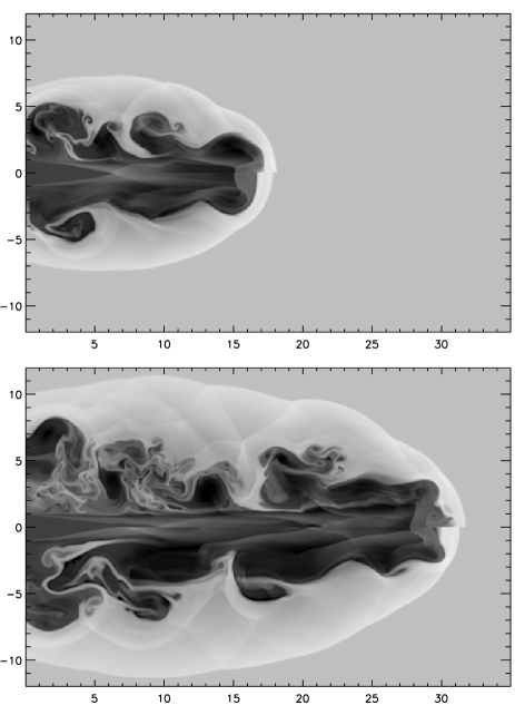
Figure 12: Gray scale images of the rest-mass density logarithm for the relativistic jet simulation at $t=40$ (top panel) and $t=80$ (bottom panel). In each panel, the HLLC (HLL) solver has been used for the upper (lower) portion of the image. The resolution is $20$ points per jet radius, corresponding to grid size of $240\times 700$ computational zones. Integration has been carried with CFL = 0.5

5 Efficiency Comparison

Previous numerical tests have shown that the quality of solution achieved with the HLLC scheme can be competitive with more complex exact or iterative non-linear Riemann solvers, see for example Martí & Müller (1996), Mignone et al. (2005). Another aspect which plays in favour of the HLLC formalism is the computational efficiency, particularly crucial in long-term simulations in two and three dimensions.

Table 1 gives the normalized CPU time required by the HLL, HLLC and approximate two-shock nonlinear Riemann solvers (for the latter see Mignone et al., 2005). All three solvers are available in the C author’s code and have been written performing similar degree of optimizations. On the contrary, the FORTRAN code for the exact solution to the Riemann problem, available from Martí & Müller (2003), was found to be more than a factor of $7$ slower than the HLL solver. We believe that this might be due to a lower degree of optimization and by the time consuming numerical integration across the rarefaction fan (Pons et al., 2000).

Test	# zones	HLL	HLLC	Riemann
# $1$	$4000$	$1$	$1.05$	$1.37$
# $2$	$4000$	$1$	$1.07$	$1.34$
# $3$	$4000$	$1$	$1.06$	$1.30$
# $4$	$4000$	$1$	$1.04$	$1.44$
R2-D	$400^{2}$	$1$	$1.03$	$1.30$

Table 1: Normalized CPU time per integration step for the first four one-dimensional shock tubes and the 2-D Riemann problem (R2-D) considered in §4.7. The two rightmost columns give the average computing time for the HLLC and two-shock nonlinear Riemann solvers normalized to the HLL time (third column). All runs were produced using the first-order scheme with $CFL=0.8$.

For illustrative purposes, we consider the first four one-dimensional tests and the two-dimensional Riemann problem. Integrations have been carried using the first-order scheme on $4000$ and $400^{2}$ zones, respectively. No optimization flags were used during the compilation.

From the table, one can easily conclude that the HLLC scheme requires little additional costs with respect to the HLL approach (between $4\%$ and $7\%$ in one dimension), while the iterative nonlinear solver is certainly more expensive, being by a factor of more than $30\%$ slower.

In making the comparison, however, one should keep in mind that HLL-type solvers are iteration-free since the underlying algorithms always require a fixed number of operations, regardless of the initial condition. On the contrary, iterative nonlinear Riemann solvers have a certain degree of adaptability since the number of iterations to achieve convergence depends on the strength of the discontinuity at the zone interface. In smooth regions of the flow, for example, fewer iterations are usually needed. This explains why the fourth test problems is particularly time consuming, since a stronger discontinuity is involved.

In this respect, a direct comparison between different Riemann solvers becomes problem-dependent and can be used only as an order-of-magnitude estimate. Conversely, we do not expect the HLLC/HLL efficiency ratio to change with increasing complexity of the flow patterns. For this reason, we believe that for problems involving rich and complex structures the trade-off between computational efficiency and quality of results is certainly worth the effort.

6 Conclusions

We have presented, for the first time, an extension of the HLLC scheme by Toro et al. (1994) to relativistic gas dynamics. The solver is robust, computationally efficient and complete, in that it considers the full wave structure in the solution to the Riemann problem. The solver retains the attractive feature of being positively conservative, typical of the HLL scheme family.

The major improvement over the simple single-state HLL solver is the ability to resolve contact and tangential discontinuities. This property has been demonstrated by direct comparisons in several one- and two-dimensional test problems, where differences are strongly evident. The results indicate that the new HLLC solver attains sharper representation of discontinuities, quantitatively similar to the exact but algebraically and computationally more intensive Riemann solver.

The additional computational cost over the traditional HLL approach is less than $8\%$ and we believe that the improved quality of results largely justifies the trade-off between the two approximate Riemann solvers.

Extension to relativistic magnetized flows will be considered in a forthcoming paper. We notice, however, that the HLLC formalism presented in this work can be easily generalized to the case of vanishing normal component of magnetic field. When this degeneracy occurs (as in the propagation of jets with toroidal magnetic field, see for example Leismann et al., 2005), in fact, the solution to the Riemann problem is entirely analogous to the non-magnetized case, since only three waves are actually involved. This extension will be presented in Mignone et al. (2005).

Finally, we mention that the relativistic HLLC scheme does not make any assumption on the equation of state, and efforts to incorporate different equations of state should be minimal.

Appendix A Proof of $\lambda_{L}\leq\lambda^{*}\leq\Lambda_{R}$

In what follows we prove some important results concerning the positivity of the our relativistic HLLC scheme. The proof is given below in A.4. Propositions A.1 through A.3 demonstrate some preliminary results.

We assume that the fastest and slowest signal velocities are computed according to the prescription given in §3.1.1, and that $\lambda_{R}>0$ and $\lambda_{L}<0$, which is the case of applicability for the intermediate fluxes (13). Obviously, the initial left and right states are supposed to be physically admissible, i.e. they belong to the set $G$ defined in §3.1.2.

Proposition A.1

$A_{R}>0$, $A_{L}<0$

We will only prove $A_{R}>0$, since the proof for $A_{L}$ is similar. For the sake of clarity, we omit the subscript $R$. Using the definition of $A$ given after equation (17) one has

$$A=(E+p)\left[\lambda\left(1-\frac{\sigma}{\Gamma}\right)-v_{x}\right]\,,$$ (40)

where $\sigma=c_{s}^{2}/\gamma^{2}$ is always positive numbers. Equation (40) is always positive for $\lambda>\lambda_{0}$, where

$$\lambda_{0}\equiv\frac{\Gamma v_{x}}{\Gamma-\sigma}\,.$$ (41)

However, according to the choice given in §3.1.1, $\lambda$ must satify

$$f(\lambda)=(\lambda-v_{x})^{2}-\frac{\sigma}{1-c_{s}^{2}}(1-\lambda^{2})\geq 0\,.$$ (42)

with $\sigma_{s}=\sigma/(1-c_{s}^{2})$. Equation (42) simply states that $\lambda$ must be greater than the root with the positive sign $\lambda_{+}$ (for the left state, $\lambda_{L}$ is always less than the root with the negative sign $\lambda_{-}$). Direct substitution of $\lambda_{0}$ from (41) into (42) shows, after some algebra, that

$$f(\lambda_{0})\leq K_{1}\left[-c_{s}^{4}+(v_{x}^{2}+2\Gamma)c_{s}^{2}-\Gamma^{2}\right]\,,$$ (43)

where the equality occurs in the limit of zero tangential velocities and $K_{1}$ is always a positive quantity. Since $1<\Gamma<2$ and $c^{2}_{s}$ has the limiting value $(\Gamma-1)$ the expression in square bracket is always negative, which means that $\lambda\geq\lambda_{+}>\lambda_{0}$. This implies that $A\equiv A_{R}$ is always positive with our choice of $\lambda\equiv\lambda_{R}$.

Since one can prove, in a similar way, that $A_{L}<0$, we have the important results that $U_{E}^{hll}=A_{R}-A_{L}>0$.

Proposition A.2

$B_{R}+A_{R}>0$, $B_{L}-A_{L}>0$.

Again we only give the proof for the right state, the other case being similar. The function $A+B$ (the subscript $R$ is omitted), with $A$ and $B$ defined after equation (17) increases linearly with $\lambda$ and is positive for $\lambda>\lambda_{0}$, where

$$\lambda_{0}=\frac{v_{x}\gamma^{2}\Gamma(v_{x}+1)+c_{s}^{2}}{\gamma^{2}\Gamma(v_{x}+1)-c_{s}^{2}}\,.$$ (44)

However, direct substitution of $\lambda_{0}$ in (42) shows, after extensive manipulations, that

$$f(\lambda_{0})=-K_{2}\Big{[}c_{s}^{4}-(1+2\Gamma)c_{s}^{2}+\gamma^{2}\Gamma^{2}(1-v_{x}^{2})\Big{]}\,,$$ (45)

where $K_{2}$ is always a positive quantity. It can be easily verified that the function in square brackets is always positive if $c_{s}^{2}\in[0,\Gamma-1]$ and $1<\Gamma<2$. Thus we must have $B_{R}/A_{R}>-1$.

Proposition A.3

$\lambda_{L}A_{R}-A_{R}<0$, $\lambda_{R}A_{L}-B_{L}>0$.

For the right state we have that

$$\lambda_{L}A-B\leq\lambda_{-}A-B\leq\left(\frac{2v}{1+\sigma_{s}}-\lambda\right)A-B\,,$$ (46)

where the last inequality follows from the fact that the two roots of equation (42) satisfy

$$\lambda_{-}=\frac{2v}{1+\sigma_{s}}-\lambda_{+}\;,\quad\textrm{and}\quad\lambda_{+}\leq\lambda\,.$$ (47)

Using the fact that $\lambda^{2}(1+\sigma_{s})\geq 2\lambda v-v^{2}+\sigma_{s}$ and that $A>0$, the last expression in equation (46) can be shown to obey the following

$$\left(\frac{2v}{1+\sigma_{s}}-\lambda\right)A-B\leq g\,,$$ (48)

where

$$g=K_{3}\Big{[}v^{2}(\Gamma-c_{s}^{2}-1)+1-\Gamma+c_{s}^{2}-2c_{s}^{2}v_{t}^{2}\Big{]}\,,$$ (49)

with $K_{3}$ being a positive quantity. The expression in square bracket in equation (49) is always negative under the same assumptions used previously. Thus we have $\lambda_{L}<B_{R}/A_{R}$ and, similarly, one can prove that $\lambda_{R}>B_{L}/A_{L}$.

Proposition A.4

$\lambda_{L}\leq\lambda^{*}\leq\lambda_{R}$.

We now show that the choice of eigenvalues given in §3.1.1 always guarantees $\lambda_{L}\leq\lambda^{*}\leq\lambda_{R}$.

The starting point is to note that the quadratic equation (18) can be more conveniently written as

$$(A_{L}\lambda^{*}-B_{L})(1-\lambda_{R}\lambda^{*})=(A_{R}\lambda^{*}-B_{R})(1-\lambda_{L}\lambda^{*})\,,$$ (50)

which defines the intersection of two quadratic functions. The parabola on the left hand side vanishes in $\lambda^{*}=1/\lambda_{R}>1$ and $\lambda^{*}=B_{L}/A_{L}<1$, whereas the parabola on the right hand side in $\lambda^{*}=1/\lambda_{L}<-1$ and $\lambda^{*}=B_{R}/A_{R}>-1$. Moreover the two quadratics have the same concavity, since $\textrm{sign}(A_{L}\lambda_{R})=\textrm{sign}(A_{R}\lambda_{L})=-1$. Thus the intersection must necessarily satisfy

$$\min\left(\frac{B_{R}}{A_{R}},\frac{B_{L}}{A_{L}}\right)\leq\lambda^{*}\leq\max\left(\frac{B_{R}}{A_{R}},\frac{B_{L}}{A_{L}}\right)\,.$$ (51)

However, for any $\lambda\in(-1,1)$ one has

$$\lambda A-B=(\lambda-v_{x})^{2}(E+p)+p(1-\lambda^{2})>0\,,$$ (52)

which, together with the results previously shown, implies that

$$\begin{array}[]{l}\displaystyle 1>\lambda_{R}>\max\left(\frac{B_{R}}{A_{R}},\frac{B_{L}}{A_{L}}\right)\,,\\ \vskip 6.0pt plus 2.0pt minus 2.0pt\cr\displaystyle-1<\lambda_{L}<\min\left(\frac{B_{R}}{A_{R}},\frac{B_{L}}{A_{L}}\right)\,.\end{array}$$ (53)

and hence

$$\lambda_{L}\leq\lambda^{*}\leq\lambda_{R}\,.$$ (54)

References

- Aloy et al. (1999) Aloy, M. A., Ibáñez, J. M. & Martí, J. M. 1999, ApJS, 122, 151
- Anile (1989) Anile, A. M. 1989, Relativistic Fluids and Magneto-fluids (Cambridge: Cambridge University Press), 55
- Balsara (1994) Balsara, D. S. 1994, J. Comput. Phys., 114, 284
- Batten et al. (1997) Batten, P., Clarke, N., Lambert, C., and Causon, D.M. 1997, SIAM J. Sci. Comput, 18, 1553
- Colella (1985) Colella, P. 1985, SIAM J. Sci. Stat. Comput., 6, 104
- Courant et al. (1928) Courant, R., Friedrichs, K. O. & Lewy, H. 1928, Math. Ann., 100, 32
- Dai & Woodward (1997) Dai, W. & Woodward, P. R. 1997, SIAM J. Sci. Comput., 18, 982
- Davis (1988) Davis, S.F. 1988, SIAM J. Sci. Statist. Comput., 9, 445
- Del Zanna & Bucciantini (2002) Del Zanna, L. & Bucciantini, N. 2002, aap, 390, 1177
- Donat et al. (1998) Donat, R., Font, J. A., Ibáñez, J. M. & Marquina, A. 1998, J. Comput. Phys., 146, 58
- Duncan & Hughes (1994) Duncan, G. C., & Hughes, P. A. 1994, apjl, 436, L119
- Einfeldt et al. (1991) Einfeldt, B., Munz, C.D., Roe, P.L., and Sjögreen, B. 1991, J. Comput. Phys., 92, 273
- Eulderink & Mellema (1995) Eulderink, F., & Mellema, G. 1995, aaps, 110, 587
- Falle & Komissarov (1996) Falle, S. A. E. G & Komissarov, S. S. 1996, mnras, 278, 586
- Gurski (2004) Gurski, K.F. 2004, SIAM J. Sci. Comput, 25, 2165
- Harten et al. (1983) Harten, A., Lax, P.D., and van Leer, B. 1983, SIAM Review, 25(1):35,61
- Lax & Liu (1998) Lax, P. D. & Liu, X.-D. 1998, SIAM J. Sci. Comput., 19, 319
- Landau & Lifshitz (1959) Landau, L. D. & Lifshitz, E. M. 1959, Fluid Mechanics (New York: Pergamon)
- Leismann et al. (2005) Leismann, T., Antón, L., Aloy, M. A., Müller, E., Martí, J. M., Miralles, J. A., & Ibáñez, J. M. 2005, aap, 436, 503
- Li (2005) Shengtai Li, 2005, J. Comput. Phys., 344-357
- Marquina et al. (1992) Marquina, A., Martí, J.M., Ibáñez, J. M., Miralles, J. A. & Donat, R. 1992, aap, 258, 566
- Martí & Müller (1994) Martí, J. M. & Müller, E. 1994, J. Fluid Mech., 258, 317
- Martí & Müller (1996) Martí, J. M. & Müller, E. 1996, J. Comput. Phys., 123, 1
- Martí et al. (1997) Martí, J. M., Müller, E., Font, J. A., Ibanez, J. M. A. & Marquina, A. 1997, apj, 479, 151
- Martí & Müller (2003) Martí, J. M. & Müller, E. 2003, Living Reviews in Relativity, 6, 7
- Mignone et al. (2005) Mignone, A., Plewa, T., and Bodo, G. 2005, ApJS, accepted
- Mignone et al. (2005) Mignone, A., Massaglia, B., and Bodo, G. 2005, in preparation
- Pons et al. (2000) Pons, J.A., Martí, J.M. & Müller, E. 2000, J. Fluid Mech., 42, 125
- Quirk (1994) Quirk, J. 1994, Int. J. Numer. Methods Fluids, 18, 555
- Rezzolla et al. (2003) Rezzolla, L., Zanotti, O., Pons, J.A., 2003, J. Fluid Mech., 479, 199
- Saltzman (1994) Saltzman, J. 1994, J. Comput. Phys., 115, 153
- Lucas-Serrano et al. (2004) Lucas-Serrano, A., Font, J. A., Ibáñez, J. M., & Martí, J. M. 2004, aap, 428, 703
- Schneider et al. (1993) Schneider, V., Katscher, U., Rischke, D.H, Waldhauser, B., Maruhn, J.A, and Munz, C.-D, 1993, J. Comput. Phys, 105, 92
- Schulz et al. (1993) Schulz-Rinne, C. W., Collins, J. P. & Glaz, H. M. 1993, SIAM J. Sci. Comp., 14, 1394
- Strang (1968) Strang, G., 1968, SIAM J. Num. Anal., 5, 506
- Taub (1948) Taub, A. H. 1948, Physical Review, 74, 328
- Toro (1997) Toro, E. F. 1997, Riemann Solvers and Numerical Methods for Fluid Dynamics, Springer-Verlag, Berlin
- Toro et al. (1994) Toro, E. F., Spruce, M., and Speares, W. 1994, Shock Waves, 4, 25