A Unified, Merger-Driven Model for the Origin of Starbursts, Quasars, the Cosmic X-Ray Background, Supermassive Black Holes and Galaxy Spheroids

Abstract

We develop an evolutionary model for starbursts, quasars, and spheroidal galaxies in which supermassive black holes play a dominant role. In this picture, mergers between gas-rich galaxies drive nuclear inflows of gas, producing intense starbursts and feeding the growth of supermassive black holes. During this phase, the black hole is heavily obscured (a “buried” quasar), but feedback energy from its growth expels the gas, rendering the black hole briefly visible as a bright, optical source (a “visible” quasar), and eventually halting accretion (a “dead” quasar). The self-regulated growth of the black hole accounts for the observed correlation between black hole mass and stellar velocity dispersion in spheroidal galaxies. We show that the quasar lifetime and obscuring column density depend on both the instantaneous and peak luminosities of the quasar, and determine this dependence using a large set of simulations of galaxy mergers varying the host galaxy properties, orbital geometry, and gas physics.

We use our fits to the lifetime and column density to deconvolve observed quasar luminosity functions and obtain the evolution of the formation rate of quasars with a certain peak luminosity, $\dot{n}(L_{\rm peak},z)$. In our model, quasars spend extended periods of time at luminosities well below their peaks, and so $\dot{n}(L_{\rm peak},z)$ has a maximum, falling off at both brighter and fainter luminosities, corresponding to the “break” in the observed quasar luminosity function. We obtain self-consistent fits to hard and soft X-ray and optical quasar luminosity functions for a model in which $\dot{n}(L_{\rm peak},z)$ varies with redshift according to pure peak luminosity evolution. From this form for $\dot{n}(L_{\rm peak},z)$, and our simulation results for the luminosity dependence of the quasar lifetime and obscuring column, we are able to reproduce many observable quantities, including: the column density distribution of both optical and X-ray selected quasar samples, the luminosity function of broad-line quasars in X-ray samples and the broad-line (Type I, Type II) fraction as a function of luminosity, the mass function of active black holes, the observed distribution of Eddington ratios at both low and high redshift, the present-day mass function of relic, inactive supermassive black holes and total black hole mass density, and the spectrum of the cosmic X-ray background. In each case, our predictions agree well with observations, matching them to higher precision than previous tunable models for quasar lifetimes and obscuration similarly fit to the luminosity function. We provide a library of Monte Carlo realizations of our modeling for comparison with a wide range of observations, using various selection criteria.

1. Introduction

The measurement of anisotropies in the cosmic microwave background (e.g. Spergel et al. 2003) combined with observations of high redshift supernovae (e.g. Riess et al. 1998, 2000; Perlmutter et al. 1999) have established a “standard model” for the Universe, in which the energy density is dominated by an unknown form driving accelerated cosmic expansion, and most of the mass is non-baryonic, in a ratio of roughly 5:1 to ordinary matter. On small scales, it is believed that structure formed through gravitational instability. In the currently favored cold dark matter (CDM) paradigm, objects grow hierarchically, with smaller ones forming first and then merging into successively larger bodies. As baryons fall into dark matter potential wells, the gas is shocked and then cools radiatively to form stars and galaxies, in a “bottom-up” progression (White & Rees 1978).

Even with the many successes of this picture, the processes underlying galaxy formation and evolution are poorly understood. For example, there has yet to be an ab initio calculation, starting from an initial state prescribed by the standard model, resulting in a population of objects that reproduces observed galaxies. However, from the same initial conditions, computer simulations have yielded a new, successful interpretation of the Lyman-alpha forest in which absorption in caused by density fluctuations in the intergalactic medium (e.g. Cen et al. 1994; Zhang et al. 1995; Hernquist et al. 1996), over many orders of magnitude in column density (e.g. Katz et al. 1996a), explicitly related to growth of structure in a CDM universe (e.g. Croft et al. 1998, 1999, 2002; McDonald et al. 2000, 2004; Hui et al. 2001; Viel et al. 2003, 2004). This suggests that the difficulties with understanding galaxy formation and evolution lie not in the initial conditions or with the description of dark matter, but rather with the physics that has been used to model the baryons.

Observations have revealed regularities in the structure of galaxies that point to some of this “missing” physics. Supermassive black holes appear to reside at the centers of most galaxies (e.g. Kormendy & Richstone 1995; Richstone et al. 1998; Kormendy & Gebhardt 2001) and the masses of these black holes are correlated with either the mass (Magorrian et al. 1998; McLure & Dunlop 2002; Marconi & Hunt 2003) or the velocity dispersion (i.e. the $M_{\rm BH}$-$\sigma$ relation: Ferrarese & Merritt 2000; Gebhardt et al. 2000; Tremaine et al. 2002) of spheroids, demonstrating a direct link between the origin of galaxies and supermassive black holes. Simulations which follow the self-regulated growth of black holes in galaxy mergers (Di Matteo et al. 2005; Springel et al. 2005a) have shown that the energy released through this process has a global impact on the structure of the merger remnant. If this conclusion applies to spheroid formation in general, the simulations demonstrate that models for the origin and evolution of galaxies must account for black hole growth and feedback in a fully self-consistent manner.

Analytical and semi-analytical modeling (Silk & Rees, 1998; Fabian, 1999; Wyithe & Loeb, 2002, 2003; Begelman & Nath, 2005) suggests that, beyond a certain threshold, feedback energy from black holes can expel gas from the centers of galaxies, shutting down accretion onto them and limiting their masses. However, these calculations usually ignore the impact of this process on star formation and therefore do not explain the link between black hole growth and spheroid formation, and furthermore make simplifying assumptions about the dynamics of such accretion. For example, the duration of black hole growth is a free parameter, which is fixed either using observational estimates or assumed to be similar to e.g. the dynamical time of the host galaxy or the $e$-folding time for Eddington-limited black hole growth $t_{S}=M_{\rm BH}/\dot{M}=4.5\times 10^{7}\,l^{-1}\,(\epsilon_{r}/0.1)\,$yr for accretion with radiative efficiency $\epsilon_{r}=L/\dot{M}c^{2}\sim 0.1$ and $l=L/L_{\rm Edd}\lesssim 1$ (Salpeter, 1964). Moreover, these studies have adopted idealized models for quasar light curves, usually corresponding to growth at a constant Eddington ratio or on-off, “light bulb,” scenarios. As we discuss below, less restrictive modeling suggests that this phase is actually more complex.

Efforts to model quasar accretion and feedback more self-consistently (e.g., Ciotti & Ostriker, 1997, 2001; Granato et al., 2004) by treating the hydrodynamical response of gas to black hole growth have generally been restricted to idealized geometries, such as spherical symmetry, employing simple models for star formation and galaxy-scale quasar fueling. However, these works have made it possible to estimate duty cycles of quasars and shown that the objects left behind have characteristics similar to those observed, with quasar feedback being a critical element in reproducing these features (e.g. Sazonov et al. 2005; Kawata & Gibson 2005; Cirasuolo et al. 2005; for a review, see Ostriker & Ciotti 2005).

Springel et al. (2005b) have incorporated black hole growth and feedback into simulations of galaxy mergers and included a multiphase model for star formation and pressurization of the interstellar gas by supernovae (Springel & Hernquist, 2003) to examine implications of these processes for galaxy formation and evolution. Di Matteo et al. (2005) and Springel et al. (2005a,b) have shown that gas inflows excited by gravitational torques during a merger both trigger starbursts and fuel rapid black hole growth. The growth of the black hole is determined by the gas supply and terminates as gas is expelled by feedback, halting accretion, leaving a dead quasar in an ordinary galaxy. The self-regulated nature of black hole growth in mergers explains observed correlations between black hole mass and properties of normal galaxies (Di Matteo et al., 2005), as well as the color distribution of ellipticals (Springel et al., 2005a). These results lend support to the view that mergers have played an important role in structuring galaxies, as advocated especially by Toomre & Toomre (1972) and Toomre (1977). (For reviews, see, e.g., Barnes & Hernquist 1992; Barnes 1998; Schweizer 1998.)

Subsequent analysis by Hopkins et al. (2005a,b,c,d) has shown that the merger simulations can account for quasar phenomena as a phase of black hole growth. Unlike what has been assumed in e.g. semi-analytical studies of quasars, the simulations predict complicated evolution for quasar lifetimes, fueling rates for black hole accretion, obscuration, and quasar light curves. The light curves were studied by Hopkins et al. (2005a, b), who showed that the self-termination process gives observable lifetimes $\sim 10^{7}\,$yr for bright optical quasars and predicts a large population of obscured sources as a natural stage of quasar evolution, as implied by observations (for a review, see Brandt & Hasinger 2005). Hopkins et al. (2005b) analyzed simulations over a range of galaxy masses and found that the quasar light curves and lifetimes are always qualitatively similar, with both the intrinsic and observed quasar lifetimes being decreasing functions of luminosity, with longer lifetimes at all luminosities for higher-mass (higher peak luminosity) systems. The dependence of the lifetime on luminosity led Hopkins et al. (2005c) to suggest a new interpretation of the quasar luminosity function, in which the steep bright-end consists of quasars radiating near the Eddington limit and is directly related to the distribution of intrinsic peak luminosities (or final black hole masses) as has been assumed previously (e.g., Small & Blandford, 1992; Haiman & Loeb, 1998; Haiman & Menou, 2000; Kauffmann & Haehnelt, 2000; Somerville et al., 2001; Tully et al., 2002; Wyithe & Loeb, 2003; Volonteri et al., 2003; Haiman, Quataert, & Bower, 2004; Croton et al., 2005), but where the shallow, faint-end of the luminosity function describes black holes growing towards or declining from peak phases of quasar activity, with Eddington ratios generally between $l\sim 0.01$ and 1. The “break” in the luminosity function corresponds directly to the peak in the distribution of intrinsic quasar properties. As argued by Hopkins et al. (2005c, d) this new interpretation of the luminosity function can self-consistently explain various properties of both the quasar and galaxy populations, connecting the origin of galaxy spheroids, supermassive black holes, and quasars.

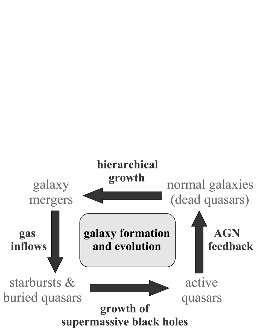
Figure 1.— Schematic representation of a “cosmic cycle” for galaxy formation and evolution regulated by black hole growth in mergers.

Motivated by these results, and earlier work by many others which we summarize below, in this paper we consider a picture for galaxy formation and evolution, illustrated schematically as a “cosmic cycle” in Figure 1, in which starbursts, quasars, and the simultaneous formation of spheroids and supermassive black holes represent connected phases in the lives of galaxies. Mergers are expected to occur regularly in a hierarchical universe, particularly at high redshifts. Those between gas-rich galaxies drive nuclear inflows of gas, triggering starbursts and fueling the growth of supermassive black holes. During most of this phase, quasar activity is obscured, but once a black hole dominates the energetics of the central region, feedback expels gas and dust, making the black hole visible briefly as a bright quasar. Eventually, as the gas is further heated and expelled, quasar activity can no longer be maintained and the merger remnant relaxes to a normal galaxy with a spheroid and a supermassive black hole. In some cases, depending on the gas content of the progenitors, the remnant may also have a disk (Springel & Hernquist 2005; Robertson et al. 2005a). The remnant will then evolve passively and would be available as a seed to repeat the above cycle. As the Universe evolves and more gas is consumed, the mergers involving gas-rich galaxies will shift towards lower masses, explaining the decline in the population of the brightest quasars from $z\sim 2$ to the present, and the remnants that are gas-poor will redden quickly owing to the termination of star formation by black hole feedback (Springel et al. 2005a), so that they resemble elliptical galaxies, surrounded by hot X-ray emitting halos (e.g. Cox et al. 2005).

There is considerable observational support for this scenario, which has led the development of this picture for the co-evolution of galaxies and quasars over recent decades. Infrared (IR) luminous galaxies are thought to be powered in part by starbursts (e.g. Soifer et al. 1984a,b; Sanders et al. 1986, 1988a,b; for a review, see e.g. Soifer et al. 1987), and the most intense examples locally, ultraluminous infrared galaxies (ULIRGs), are invariably associated with mergers (e.g. Allen et al. 1985; Joseph & Wright 1985; Armus et al. 1987; Kleinmann et al. 1988; Melnick & Mirabel 1990; for reviews, see Sanders & Mirabel 1996 and Jogee 2004). Radio observations show that ULIRGs have large, central concentrations of dense gas (e.g. Scoville et al. 1986; Sargent et al. 1987, 1989), providing a fuel supply to feed black hole growth. Indeed, some ULIRGs have “warm” IR spectral energy distributions (SEDs), suggesting that they harbor buried quasars (e.g. Sanders et al. 1988c), an interpretation strengthened by X-ray observations demonstrating the presence of two non-thermal point sources in NGC6240 (Komossa et al., 2003), which are thought to be supermassive black holes that are heavily obscured at visual wavelengths (e.g. Gerssen et al. 2004; Max et al. 2005, Alexander et al. 2005a,b). These lines of evidence, together with the overlap between bolometric luminosities of ULIRGs and quasars, indicate that quasars are the descendents of an infrared luminous phase of galaxy evolution caused by mergers (Sanders et al. 1988a), an interpretation supported by observations of quasar hosts (e.g. Stockton 1978; Heckman et al. 1984; Stockton & MacKenty 1987; Stockton & Ridgway 1991; Hutchings & Neff 1992; Bahcall et al. 1994, 1995, 1997; Canalizo & Stockton 2001).

However, many of the physical processes that connect the phases of evolution in Figure 1 are not well understood. Early simulations showed that mergers produce objects resembling galaxy spheroids (e.g. Barnes 1988, 1992; Hernquist 1992, 1993a) and that if the progenitors are gas-rich, gravitational torques funnel gas to the center of the remnant (e.g. Barnes & Hernquist 1991, 1996), producing a starburst (e.g. Mihos & Hernquist 1996), but these works did not explore the relationship of these events to black hole growth and quasar activity. While a combination of arguments based on time variability and energetics suggests that quasars are produced by the accretion of gas onto supermassive black holes in the centers of galaxies (e.g. Salpeter 1964; Zel’dovich & Novikov 1964; Lynden-Bell 1969), the mechanism that provides the trigger to fuel quasars therefore remains uncertain. Furthermore, there have been no comprehensive models that describe the transition between ULIRGs and quasars that can simultaneously account for observed correlations like the $M_{\rm BH}$-$\sigma$ relation.

Here, we study these relationships using numerical simulations of galaxy mergers that account for the consequences of black hole growth. In our simulations, black holes accrete and grow throughout a merger event, producing complex, time-varying quasar activity. Quasars reach a peak luminosity, $L_{\rm peak}$, during the “blowout” phase of evolution where feedback energy from black hole growth begins to drive away the gas, eventually slowing accretion. Prior to and following this brief period of peak activity, quasars radiate at instantaneous luminosities, $L$, with $L<L_{\rm peak}$. However, we show that even with this complex behavior, the global characteristics that determine the observed properties of quasars, i.e. lifetimes, light curves, and obscuration, can be expressed as functions of $L$ and $L_{\rm peak}$, allowing us to make predictions for quasar populations that agree well with observations, supporting the scenario sketched in Figure 1.

In § 2, we discuss our methodology and show how the quasar lifetimes and obscuration from our simulations can be expressed as functions of the instantaneous and peak luminosities of quasars. We also define a set of commonly adopted models for the quasar lifetime and obscuration against which we compare our predictions throughout. In § 3, we apply our models to the quasar luminosity function, using the observed luminosity function to determine the distribution of quasar peak luminosities, and show that this allows us to simultaneously reproduce the hard X-ray, soft X-ray, and optical quasar luminosity functions at all redshifts $z\lesssim 3$, and the distribution of column densities in both optical and X-ray samples. In § 4, we determine the time in our simulations when quasars will be observable as broad-line objects, and use this to predict the broad-line luminosity function and fraction of broad-line objects in quasar samples, as a function of luminosity, as well as the mass function of low-redshift, active broad-line quasars. In § 5, we estimate the distribution of Eddington ratios in our simulations as a function of luminosity, and infer Eddington ratios in observed samples at different redshifts. In § 6, we use our modeling to predict both the mass distribution and total density of present-day relic supermassive black holes, and describe their evolution with redshift. In § 7, we similarly apply this model to predict the integrated cosmic X-ray background spectrum, accounting for the observed spectrum from $\sim 1-100$ keV. In § 8, we discuss the primary qualitative implications of our results and propose falsifiable tests of our picture. Finally, in § 9, we conclude and suggest directions for future work.

Throughout, we adopt a $\Omega_{\rm M}=0.3$, $\Omega_{\Lambda}=0.7$, $H_{0}=70\,{\rm km\,s^{-1}\,Mpc^{-1}}$ ($h=0.7$) cosmology.

2. The Model: Methodology

Our model of quasar evolution has several elements, which we summarize here and describe in greater detail below.

• In what follows, a “quasar” is taken to mean the course of black hole activity in a single merger event. We use the term “quasar lifetime” to refer to the time spent by such a quasar at a given luminosity or fraction of the quasar peak luminosity, integrated over all black hole activity in a single merger event. This is not meant to suggest that this would constitute the entire accretion history of a black hole – a given black hole may have multiple “lifetimes” triggered by different mergers, with each merger in principle fueling a distinct “quasar” with its own lifetime. There is no a priori luminosity threshold for quasar activity – the time history can include various epochs at low luminosities and accretion rates.

• We model the galaxy mergers using hydrodynamical simulations, varying the orbital parameters of the encounter, the internal properties of the merging galaxies, prescriptions for the gas physics, initial “seed” black hole masses of the merging systems, and numerical resolution of the simulations. The black hole accretion rate is determined from the surrounding gas (smoothed over the scale of our spatial resolution, reaching $20\,$pc in the best cases), i.e. the density and sound speed of the gas, and its motion relative to the black hole, using Eddington-limited, Bondi-Hoyle-Lyttleton accretion theory. The black hole radiates with a canonical efficiency $\epsilon_{r}=0.1$ corresponding to a standard Shakura & Sunyaev (1973) thin disk, and we assume that $\sim 5\%$ of this radiated luminosity is deposited as thermal energy into the surrounding gas, weighted by the SPH smoothing kernel (which has a $\sim r^{-2}$ profile) over the scale of the spatial resolution. This scale is such that we cannot resolve the complex accretion flow immediately around the black hole, but we adopt this prescription because: (1) it reproduces the observed slope and normalization in the $M_{\rm BH}-\sigma$ relation (Di Matteo et al. 2005), (2) it follows from observations, based on estimates of the energy contained in highly-absorbed UV portion of the quasar SED (e.g., Elvis et al., 1994; Telfer et al., 2002), (3) it follows from theoretical considerations of momentum coupling to dust grains in the dense gas very near the quasar (Murray et al., 2005) and hydrodynamical simulations of small-scale radiative heating from quasar accretion (Ciotti & Ostriker, 2001), and (4) even if the feedback is initially highly collimated, a driven wind or shock in a dense region such as the center of the merging galaxies will rapidly isotropize, so long as it is decelerated by gravity and the surrounding medium, allowing the high sound speed within the shock to equalize angle-dependent pressure variations (e.g., Koo & McKee, 1990), and furthermore initial local distortions will be washed away in favor of triaxial structure determined by the large-scale density gradients (Bisnovatyi-Kogan & Silich, 1991), as occurs in our simulations.

• For each of our merger simulations, we compute the bolometric black hole luminosity and column density along $\sim 1000$ lines of sight to the black hole(s) (evenly spaced in solid angle), as a function of time from the beginning of the simulation until the system has relaxed for $\sim 1\,$Gyr after the merger.

• We bin different merger simulations by $L_{\rm peak}$, the peak bolometric luminosity of the black hole in the simulation, and the conditional distributions of luminosity, $P(L|L_{\rm peak})$, and column density, $P(N_{\rm H}|L,\,L_{\rm peak})$, are computed using all simulations that fall into a given bin in $L_{\rm peak}$. The final black hole mass (black hole mass at the end of the individual merger – subsequent mergers and quasar episodes could further increase the black hole mass) is approximately $M_{\rm BH}^{f}\approx M_{\rm Edd}(L_{\rm peak})$ (but not exactly, see § 2.4), so we obtain similar results if we bin instead by $M_{BH}^{f}$. Our calculation of $M_{BH}^{f}(L_{\rm peak})$ allows us to express our conditional distributions of luminosity and column density in terms of either peak luminosity or final black hole mass. Critically, we find that expressed in terms of $L_{\rm peak}$ or $M_{\rm BH}^{f}$, there is no systematic dependence in the quasar evolution on the varied merger simulation properties – this allows us to calculate a large number of observables in terms of $L_{\rm peak}$ or $M_{\rm BH}^{f}$ without the large systematic uncertainties inherent in attempting to directly estimate e.g. quasar light curves in terms of host galaxy mass, gas fraction, multiphase pressurization of the interstellar medium, orbital parameters and merger stage, and other variables.

• The observed quasar luminosity function is the convolution of the time a given quasar spends at some observed luminosity with the rate at which such quasars are created. Knowing the distributions $P(L|L_{\rm peak})$ and $P(N_{\rm H}|L,\,L_{\rm peak})$, we can calculate the time spent by a quasar with some $L_{\rm peak}$ at an observed luminosity in a given waveband. We use this to fit to observational estimates of the bolometric quasar luminosity function $\phi(L)$, de-convolving these quantities to determine the function $\dot{n}(L_{\rm peak})$; i.e. the rate at which quasars of a given peak luminosity must be created or activated (triggered in mergers) in order to reproduce the observed bolometric luminosity function.

• Given these inputs, we determine the joint distribution in instantaneous luminosity and black hole mass, column density distribution, peak luminosity and final black hole mass, as a function of redshift, i.e. $n(L,\,L_{\nu},\,M_{\rm BH},\,N_{\rm H},\,L_{\rm peak},\,M_{\rm BH}^{f}\ |\ z)$, at all redshifts where the observed quasar luminosity function can provide the necessary constraint. From this joint distribution, we can compute, for example, luminosity functions in other wavebands, conditional column density distributions, active black hole mass functions and Eddington ratio distributions, and relic black hole mass functions and cosmic backgrounds. We can compare each of these results to those determined using simpler models for either the quasar lifetime or column density distributions; in § 2.5 we describe a canonical set of such models, to which we compare throughout this paper.

2.1. The Simulations

The simulations were performed with GADGET-2 (Springel, 2005), a new version of the parallel TreeSPH code GADGET (Springel, Yoshida, & White, 2001). GADGET-2 is based on a fully conservative formulation (Springel & Hernquist, 2002) of smoothed particle hydrodynamics (SPH), which maintains simultaneous energy and entropy conservation when smoothing lengths evolve adaptively (for a discussion, see e.g., Hernquist 1993b, O’Shea et al. 2005). Our simulations account for radiative cooling, heating by a UV background (as in Katz et al. 1996b, Davé et al. 1999), and incorporate a sub-resolution model of a multiphase interstellar medium (ISM) to describe star formation and supernova feedback (Springel & Hernquist, 2003). Feedback from supernovae is captured in this sub-resolution model through an effective equation of state for star-forming gas, enabling us to stably evolve disks with arbitrary gas fractions (see, e.g. Springel et al. 2005b; Robertson et al. 2004). In order to investigate the consequences of supernova feedback over a range of conditions, we employ the scheme of Springel et al. (2005b), introducing a parameter $q_{\rm EOS}$ to interpolate between an isothermal equation of state ($q_{\rm EOS}=0$) and the full multiphase equation of state ($q_{\rm EOS}=1$) described above.

Supermassive black holes (BHs) are represented by “sink” particles that accrete gas at a rate $\dot{M}$ estimated using an Eddington-limited version of Bondi-Hoyle-Lyttleton accretion theory (Bondi 1952; Bondi & Hoyle 1944; Hoyle & Lyttleton 1939). The bolometric luminosity of the black hole is $L_{\rm bol}=\epsilon_{r}\dot{M}c^{2}$, where $\epsilon_{r}=0.1$ is the radiative efficiency. We assume that a small fraction (typically $\approx 5\%$) of $L_{\rm bol}$ couples dynamically to the surrounding gas, and that this feedback is injected into the gas as thermal energy, as described above.

We have performed several hundred simulations of colliding galaxies, varying the numerical resolution, the orbit of the encounter, the masses and structural properties of the merging galaxies, initial gas fractions, halo concentrations, and the parameters describing star formation and feedback from supernovae and black hole growth. This large set of simulations allows us to investigate merger evolution for a wide range of galaxy properties and to identify any systematic dependence of our modeling. The galaxy models are described in Springel et al. (2005b), and we briefly review their properties here.

The progenitor galaxies in our simulations have virial velocities $V_{\rm vir}=80,$ $113,$ $160,$ $226,$ $320,$ ${\rm and}\ 500\,{\rm km\,s^{-1}}$. We consider cases with gas equation of state parameters $q_{\rm EOS}=0.25$ (moderately pressurized, with a mass-weighted temperature of star-forming gas $\sim 10^{4.5}{\rm K}$) and $q_{\rm EOS}=1.0$ (the full, “stiff” Springel-Hernquist equation of state, with a mass-weighted temperature of star-forming gas $\sim 10^{5}{\rm K}$), and initial disk gas fractions (by mass) of $f_{\rm gas}=0.2,$ $0.4,$ $0.8,$ ${\rm and}\ 1.0$. Finally, we scale these models with redshift, altering the physical sizes of the galaxy components and the dark matter halo concentration in accord with cosmological evolution (Mo, Mao & White, 1998). Details are provided in Robertson et al. (2005b), and here we consider galaxy models scaled appropriately to resemble galaxies of the same $V_{\rm vir},f_{\rm gas},{\rm and}\ q_{\rm EOS}$ at redshifts $z_{\rm gal}=0,$ $2,$ $3,$ ${\rm and}\ 6$.

For each simulation, we generate two stable, isolated disk galaxies, each with an extended dark matter halo with a Hernquist (1990) profile, motivated by cosmological simulations (e.g. Navarro et al. 1996; Busha et al. 2004) and observations of halo properties (e.g. Rines et al. 2002, 2002, 2003, 2004), an exponential disk of gas and stars, and (optionally) a bulge. The galaxies have masses $M_{\rm vir}=V_{\rm vir}^{3}/(10GH_{0})$ for $z_{\rm gal}=0$, with the baryonic disk having a mass fraction $m_{\rm d}=0.041$, the bulge (when present) has a mass fraction $m_{\rm b}=0.0136$, and the rest of the mass is in dark matter typically with a concentration parameter $c=9.0$. The disk scale-length is computed based on an assumed spin parameter $\lambda=0.033$, chosen to be near the mode in the observed $\lambda$ distribution (Vitvitska et al., 2002), and the scale-length of the bulge is set to $0.2$ times the resulting value. In Hopkins et al. (2005a), we describe our analysis of simulation A3, one of our set with $V_{\rm vir}=160\,{\rm km\,s^{-1}},\ f_{\rm gas}=1.0,\ q_{\rm EOS}=1.0,\ {\rm and}\ z_{\rm gal}=0$, a fiducial choice with a rotation curve and mass similar to the Milky Way, and Hopkins et al. (2005b, c, d) used a set of simulations with the same parameters but varying $V_{\rm vir}=80,$ $113,$ $160,$ $226,$ ${\rm and}\ 320\,{\rm km\,s^{-1}}$, which we refer to below as runs A1, A2, A3, A4, and A5, respectively.

Typically, each galaxy is initially composed of 168000 dark matter halo particles, 8000 bulge particles (when present), 24000 gas and 24000 stellar disk particles, and one BH particle. We vary the numerical resolution, with many of our simulations using instead twice as many particles in each galaxy, and a subset of simulations with up to 128 times as many particles. We vary the initial seed mass of the black hole to identify any systematic dependence of our results on this choice. In most cases, we choose the seed mass either in accord with the observed $M_{\rm BH}$-$\sigma$ relation or to be sufficiently small that its presence will not have an immediate dynamical effect. Given the particle numbers employed, the dark matter, gas, and star particles are all of roughly equal mass, and central cusps in the dark matter and bulge profiles are reasonably well resolved (see Fig 2. in Springel et al. 2005b). The galaxies are then set to collide from a zero energy orbit, and we vary the inclinations of the disks and the pericenter separation.

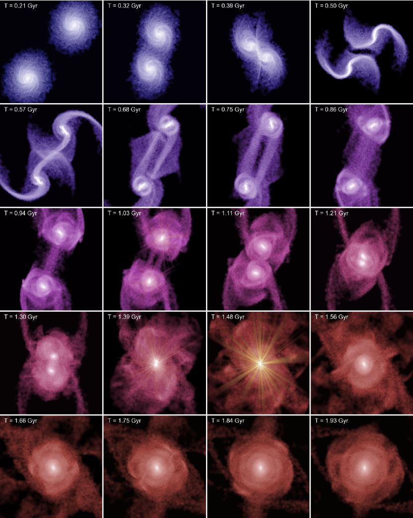
Figure 2.— Time sequence from one of our merger simulations ($V_{\rm vir}=160\,{\rm km\,s^{-1}}$, initial gas fraction 20%). Each panel is $80\,h^{-1}{\rm kpc}$ on a side and shows the simulation time in the upper left corner. Brightness of individual pixels gives the logarithm of the projected stellar mass density, while color hue indicates the baryonic gas fraction, from 20% (blue) to less than 5% (red). At $T=1.03$, $1.39$ and $1.48\,{\rm Gyr}$, when the black hole could be seen as an optical quasar, nuclear point sources are shown, providing a representation of the relative luminosities of stars and the quasar at these times.

A representative example of the behavior of the simulations is provided in Figure 2, which shows the time sequence of a merger involving two bulge-less progenitor galaxies with virial velocities of $160\,{\rm km\,s^{-1}}$ and initial gas fractions of 20%. During the merger, gas is driven to the galaxy centers by gravitational tides, fueling nuclear starbursts and black hole growth. The quasar activity is short-lived and peaks twice in this merger, both during the first encounter and the final coalescence of the galaxies. To illustrate the bright, optically observable phase(s) of quasar activity which we identify below, we have added nuclear point sources in the center at the position(s) of the black hole(s) at times $T=1.03$, $1.39$ and $1.48\,{\rm Gyr}$, generating a surface density in correspondence to the relative luminosities of stars and quasar at these times. At other times, the accretion activity is either obscured or the black hole accretion rate is negligible. To make the appearance of the quasar visually more apparent, we have put a small part of its luminosity in “rays” around the quasar. These rays are artificial and are only a visual guide.

2.2. Column Densities & Quasar Attenuation

From the simulation outputs, we determine the obscuration of the black hole as a function of time during a merger by calculating the column density to a distant observer along many lines of sight. Typically, we generate $\sim 1000$ radial lines-of-sight (rays), each with its origin at the black hole location and with directions uniformly spaced in solid angle ${\rm d}\cos{\theta}\,{\rm d}\phi$. For each ray, we begin at the origin and calculate and record the local gas properties using the SPH formalism and move a distance along the ray $\Delta r=\eta h_{\rm sml}$, where $\eta\leq 1$ and $h_{\rm sml}$ is the local SPH smoothing length. The process is repeated until a ray is sufficiently far from the origin ($\gtrsim 100$ kpc) that the column has converged. We then integrate the gas properties along a particular ray to give the line-of-sight column density and mean metallicity. We have varied $\eta$ and find empirically that gas properties along a ray converge rapidly and change smoothly for $\eta=0.5$ and smaller. We similarly vary the number of rays and find that the distribution of line-of-sight properties converges for $\gtrsim 100$ rays.

From the local gas properties, we use the multiphase model of the ISM described in Springel & Hernquist (2003) to determine the mass fraction in “hot” (diffuse) and “cold” (molecular and HI cloud core) phases of dense gas and, assuming pressure equilibrium, we obtain the local density of the hot and cold phases and their corresponding volume filling factors. The resulting values are in rough agreement with those of McKee & Ostriker (1977). Given a temperature for the warm, partially ionized component of the hot-phase $\sim 8000\,{\rm K}$, determined by pressure equilibrium, we further calculate the neutral fraction of this gas, typically $\sim 0.3-0.5$. We denote the neutral and total column densities as $N_{\rm H\,I}$ and $N_{\rm H}$, respectively. Using only the hot-phase density allows us to place an effective lower limit on the column density along a particular line of sight, as it assumes a given ray passes only through the diffuse ISM, with $\gtrsim 90\%$ of the mass of the dense ISM concentrated in cold-phase “clumps.” Given the small volume filling factor ($<0.01$) and cross section of cold clouds, we expect that the majority of sightlines will pass only through the “hot-phase” component.

Using $L_{\rm bol}=\epsilon_{r}\dot{M}c^{2}$, we model the intrinsic quasar continuum SED following Marconi et al. (2004), based on optical through hard X-ray observations (e.g., Elvis et al., 1994; George et al., 1998; Vanden Berk et al., 2001; Perola et al., 2002; Telfer et al., 2002; Ueda et al., 2003; Vignali et al., 2003), with a reflection component generated by the PEXRAV model (Magdziarz & Zdziarski, 1995). This yields, for example, a B-band luminosity $\log{(L_{B}/L_{\sun})}=0.80-0.067\mathcal{L}+0.017\mathcal{L}^{2}-0.0023\mathcal{L}^{3}$, where $\mathcal{L}=\log{(L_{\rm bol}/L_{\sun})}-12$, and we take $\lambda_{B}=4400\,$Å, but as we model the entire intrinsic SED we can determine the bolometric correction in any frequency interval.

We then use a gas-to-dust ratio to determine the extinction along a given line of sight at optical frequencies. Observations suggest that the majority of reddened quasars have reddening curves similar to that of the Small Magellanic Cloud (SMC; Hopkins et al. 2004, Ellison et al. 2005), which has a gas-to-dust ratio lower than the Milky Way by approximately the same factor as its metallicity (Bouchet et al., 1985). Hence, we consider both a gas-to-dust ratio equal to that of the Milky Way, $(A_{B}/N_{\rm H\,I})_{\rm MW}=8.47\times 10^{-22}\,{\rm cm^{2}}$, and a gas-to-dust ratio scaled by metallicity, $A_{B}/N_{\rm H\,I}=(Z/0.02)(A_{B}/N_{\rm H\,I})_{\rm MW}$. In both cases we use the SMC-like reddening curve of Pei (1992). The form of the correction for hard X-ray (2-10 keV) and soft X-ray (0.5-2 keV) luminosities is similar to that of the B-band luminosity. We calculate extinction at X-ray frequencies (0.03-10 keV) using the photoelectric absorption cross sections of Morrison & McCammon (1983) and non-relativistic Compton scattering cross sections, similarly scaled by metallicity. In determining the column density for photoelectric X-ray absorption, we ignore the inferred ionized fraction of the gas, as it is expected that the inner-shell electrons which dominate the photoelectric absorption edges will be unaffected in the temperature ranges of interest. We do not perform a full radiative transfer calculation, and therefore do not model scattering or re-processing of radiation by dust in the infrared.

For a full comparison of quasar lifetimes and column densities obtained varying our calculation of $N_{\rm H}$, we refer to Hopkins et al. (2005b) (see their Figures 1, 5, & 6), and note their conclusion that, after accounting for clumping of most mass in the dense ISM in cold-phase structures, the column density does not depend sensitively on our assumptions for the small-scale physics of the ISM and obscuration – typically, the uncertainties in the resulting quasar lifetime as a function of luminosity are a factor $\sim 2$ at low luminosities in the B-band, and smaller in e.g. the hard X-ray. Because our determination of the quasar luminosity functions is similar using the hard X-ray data alone or the hard X-ray, soft X-ray, and optical data simultaneously, the added uncertainties in our calculation of $\dot{n}(L_{\rm peak})$ in § 3.2 below owing to the uncertainty in our $N_{\rm H}$ calculation are small compared to the uncertainties owing to degeneracies in the fitting procedure and uncertain bolometric corrections.

2.3. The $N_{\rm H}$ Distribution as a Function of Luminosity

Next, we consider the distribution of column densities as a function of both the instantaneous and peak quasar luminosities. For each simulation, we consider $N_{\rm H}$ values at all times with a given bolometric luminosity $L$ (in some logarithmic interval in $L$), and determine the distribution of column densities at that $L$ weighted by the total time along all sightlines with a given $N_{\rm H}$. At each $L$, we approximate the simulated distribution and fit it to a lognormal form,

$$P(N_{H})=\frac{1}{\sigma_{N_{H}}\sqrt{2\pi}}\,\exp\left[\frac{-\log^{2}(N_{H}/\bar{N}_{H})}{2\sigma_{N_{H}}^{2}}\right].$$ (1)

This provides a good fit for all but the brightest luminosities, where quasar feedback becomes important driving the “blowout” phase, and the quasar sweeps away surrounding gas and dust to become optically observable.

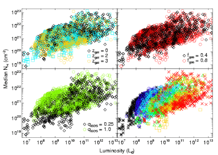
Figure 3.— The median fitted total (neutral and ionized) column density $\bar{N}_{H}$ at each luminosity $L$ in the snapshots from our series of simulations described in § 2. We compare changing concentrations and halo properties with redshift $z_{\rm gal}$ (upper left), gas fractions $f_{\rm gas}$ (upper right), the equation of state parameter $q_{\rm EOS}$ (lower left), and virial velocity $V_{\rm vir}$ (lower right). At lower right, simulations with $V_{\rm vir}=80,113,160,226,320,{\rm and}\ 500\,{\rm km\,s^{-1}}$ are shown as black asterisks, purple dots, red diamonds, green triangles, yellow squares, and red crosses, respectively. Other than a possible weak sensitivity to $q_{\rm EOS}$, the column density distribution as a function of luminosity shows no systematic dependence on any of the varied simulation parameters.

We show the resulting median column density $\bar{N}_{H}$ at each luminosity $L$ in Figure 3. In the upper left panel, simulations with $z_{\rm gal}=0$ are shown in black, those with $z_{\rm gal}=2$ in blue, and those with $z_{\rm gal}=3$ in yellow. In the upper right, simulations with $f_{\rm gas}=0.4$ are shown in black, those with $f_{\rm gas}=0.8$ in red. In the lower left, simulations with $q_{\rm EOS}=0.25$ are shown in black, those with $q_{\rm EOS}=1.0$ in green. And in the lower right, simulations with $V_{\rm vir}=80,113,160,226,320,{\rm and}\ 500\,{\rm km\,s^{-1}}$ are shown as black asterisks, purple dots, red diamonds, green triangles, yellow squares, and red crosses, respectively. Simulations with other values for these parameters (not shown for clarity, but see e.g. Hopkins et al. [2005d]) show similar trends.

While the increase in typical $N_{\rm H}$ values with luminosity appears to contradict observations suggesting that the obscured fraction decreases with luminosity, this is because the relationship shown above is dominated by quasars in growing, heavily obscured phases. In these stages, the relationship between column density and luminosity is a natural consequence of the fact that both are fueled by strong gas flows into the central regions of the galaxy – more gas inflow means higher luminosities, but also higher column densities. During these phases, the lognormal fits to column density as a function of instantaneous and peak luminosity presented in this section are reasonable approximations, but they break down in the brightest, short-lived stages of merger activity when the quasar rapidly heats the surrounding gas and drives a powerful wind, lowering the column density, resulting in a bright, optically observable quasar. Including in greater detail the effects of quasar blowout during the final stages of its growth in § 4, we find that this modeling actually predicts the observed decrease in obscured fraction with luminosity.

The relationship between $N_{\rm H}$ and $L$ shows no strong systematic dependence on any of the simulation parameters considered. At most, there is weak sensitivity to $q_{\rm EOS}$, in the sense that the simulations with $q_{\rm EOS}=1.0$ have slightly larger column densities at a given luminosity than those with $q_{\rm EOS}=0.25$. We derive an analytical model relating both the observed column density and quasar luminosity to the inflowing mass of gas in Hopkins et al. (2005d), by assuming that while it is growing, the black hole mass is proportional to the inflowing gas mass in the galaxy core (which ultimately produces the Magorrian et al. [1998] relation between black hole and bulge mass), and assuming Bondi accretion, with obscuration along a sightline through this (spherically symmetric) gas inflow. Such a model gives the observed correlation between $N_{\rm H}$ and $L$, and explains the weak dependence of the column density-luminosity relation on the ISM gas equation of state. The assumptions above give a relationship of the form

$$N_{\rm H}\sim f_{0}\,\frac{1}{m_{H}R_{c}}\,\Bigl{(}\frac{c_{s}}{c}\Bigr{)}\,\Bigl{(}\frac{cL}{G^{2}}\Bigr{)}^{1/3},$$ (2)

where $f_{0}\sim 50$ is a dimensionless factor depending on the radiative efficiency, mean molecular weight, density profile, and assumed $M_{\rm BH}-\sigma$ relation; $m_{H}$ is the mass of hydrogen; $R_{c}$ the radius of the galaxy core ($\sim 100\,{\rm pc}$); and $c_{s}$ the effective sound speed in the central regions of the galaxy. A $q_{\rm EOS}=1.0$ equation of state, with a higher effective temperature, results in a factor of $\approx 2$ larger sound speed in the densest regions of the galaxy than a $q_{\rm EOS}=0.25$ equation of state (Springel et al., 2005b), explaining the weak trend seen. In any event, the dependence is small compared to the intrinsic scatter for either equation of state in the value of $\bar{N}_{H}$ at a given luminosity, and further weakens at high luminosity, so it can be neglected. What may appear to be a systematic offset in $\bar{N}_{H}$ with $V_{\rm vir}$ is actually just a tendency for larger $V_{\rm vir}$ systems to be at higher luminosities; there is no significant change in the dependence of $N_{\rm H}$ on $L$.

We use our large set of simulations to improve our fits (relative to those of Hopkins et al. 2005d) to the $N_{\rm H}$ distribution as a function of instantaneous and peak luminosities. Looking at individual simulations, there appears to be a “break” in the power-law scaling of $\bar{N}_{H}$ with $L$ at $L\sim 10^{11}\,L_{\sun}$. We find that the best fit to the median column density $\bar{N}_{H}$ is then

$$\bar{N}_{H}=\left\{\begin{array}[]{ll}10^{22.8}\,{\rm cm^{-2}}\Bigl{(}\frac{L}{L_{\rm peak}}\Bigr{)}^{0.54}&\mathrm{if\ }L<10^{11}\,L_{\sun}\\ 10^{21.9}\,{\rm cm^{-2}}\Bigl{(}\frac{L}{10^{11}\,L_{\sun}}\Bigr{)}^{0.43}&\mathrm{if\ }L>10^{11}\,L_{\sun}.\end{array}\right.$$ (3)

Either of these two relations provides an acceptable fit to the plotted $\bar{N}_{H}$ distribution if applied to the entire luminosity range ($\chi^{2}/\nu\approx 2.8,\,3.2$ for the first and second relations, respectively), but their combination provides a significantly better fit ($\chi^{2}/\nu\approx 1.5$), although it is clear from the large scatter in $\bar{N}_{H}$ values that any such fit is a rough approximation. Despite the complicated form of this equation, it is, in practice, similar to our $\bar{N}_{H}\propto L^{0.35}$ fit from previous work and $\bar{N}_{H}\propto L^{1/3}$ analytical scaling over the range of relevant luminosities, but is more accurate by a factor $\sim 2-3$ at low ($\lesssim 10^{9}\,L_{\sun}$) luminosities. For comparison, however, we do consider this simpler form for $N_{\rm H}(L)$ as well as our more accurate fit above in our subsequent analysis, and find that it makes little difference to most observable quasar properties. At the highest luminosities, near the peak luminosities of the brightest quasars, the scatter about these fitted median $\bar{N}_{H}$ values increases, and as noted above the impact of the quasar in expelling surrounding gas becomes important and column densities vary rapidly. We consider this “blowout” phase in more detail in § 4.

We find that any dependence of $\sigma_{N_{H}}$ (the fitted lognormal dispersion) on $L$ or $L_{\rm peak}$ is not statistically significant, with approximately constant $\sigma_{N_{H}}\approx 0.4$ for individual simulations. We similarly find no systematic dependence of $\sigma_{N_{H}}$ on any of our varied simulation parameters. However, it is important to note that while the dispersion in $N_{\rm H}$ for an individual simulation is $\sigma_{N_{H}}\approx 0.4$, the dispersion in $\bar{N}_{H}$ across all simulations at a given luminosity is large, $\sim 1$ dex. Thus, we fit the effective $\sigma_{N_{H}}$ at a given luminosity for the distribution of quasars and find it is $\sigma_{N_{H}}\approx 1.2$. Although we have slightly revised our fits for greater accuracy at low luminosities, we note that this relation is shallower than the relation $N_{\rm H}\propto L$ roughly expected if $M_{\rm BH}$ is constant ($L\propto\rho\propto N_{\rm H}$) or $L\propto M_{\rm BH}$ always, and strongly contrasts with unification models which predict static obscuration, or evolutionary models in which $N_{\rm H}$ is independent of $L$ up to some threshold (e.g., Fabian, 1999).

2.4. Quasar Lifetimes & Sensitivity to Simulation Parameters

We define the luminosity-dependent quasar lifetime $t_{Q}=t_{Q}(L_{\rm min})$ as the time a quasar has a luminosity above a certain reference luminosity $L_{\rm min}$; i.e. the total time the quasar shines at $L\geq L_{\rm min}$. For ease of comparison across frequencies, we measure the lifetime in terms of the bolometric luminosity, $L$, rather than e.g. the B-band luminosity. Knowing the distribution of column densities $N_{\rm H}$ as a function of luminosity and system properties (see § 2.3), we can then analytically or numerically calculate the distribution of observed lifetimes at any frequency if we know this intrinsic lifetime. Below $\sim 1$ Myr, our estimates of $t_{Q}$ become uncertain owing to the effects of quasar variability and our inability to resolve the local small-scale physics of the ISM, but this is significantly shorter than even the most rapid timescales $\sim 10$ Myr of substantial quasar evolution.

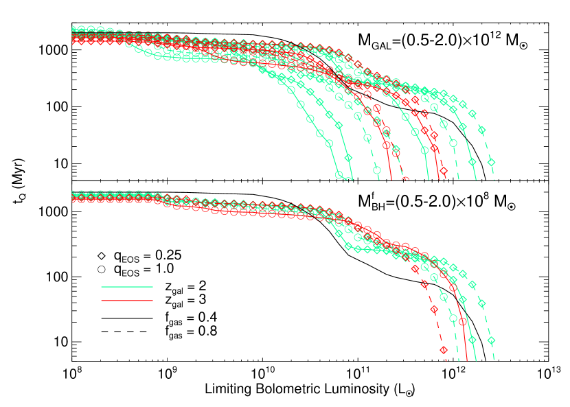
Figure 4.— Integrated intrinsic quasar lifetime above a given reference bolometric luminosity, $t_{Q}(L)$, as a function of luminosity for simulations with host galaxies with total mass (top panel) $M_{\rm gal}=0.5-2.0\times 10^{12}\,M_{\sun}$, and simulations with final black hole masses (bottom panel) $M^{f}_{\rm BH}=0.5-2.0\times 10^{8}\,M_{\sun}$ (i.e. similar peak luminosity $L_{\rm peak}\sim 10^{12}\,L_{\sun}$). The simulations cover a range in equation of state parameter $q_{\rm EOS}$, initial disk gas fraction $f_{\rm gas}$, galaxy redshift (for scaling of halo properties) $z_{\rm gal}$, and virial velocities $V_{\rm vir}=113-160\,{\rm km\,s^{-1}}$. The black line in both cases is for a merger involving Milky Way-like galaxy models, which we refer to as A3, with $f_{\rm gas}=1,\,q_{\rm EOS}=1,\,z_{\rm gal}=0,\ {\rm and}\ V_{\rm vir}=160\,{\rm km\,s^{-1}}$.

As before, we use our diverse sample of simulations to test for systematic effects in our parameterization of the quasar lifetime. Figure 4 shows the quasar lifetime as a function of reference luminosity $L_{\rm min}$ for both a set of simulations with similar total galaxy mass, $M_{\rm gal}\approx 10^{12}\,M_{\sun}$, and similar final black hole mass (i.e. similar peak quasar luminosity), $M^{f}_{\rm BH}\approx 10^{8}\,M_{\sun}$. In each case, the simulations cover a range in $q_{\rm EOS},$ $f_{\rm gas},$ $z_{\rm gal},$ ${\rm and}\ V_{\rm vir}$.

As Figure 4 demonstrates, at a given $M_{\rm gal}$, there is a wide range of lifetimes, with a systematic dependence on several quantities. For example, for fixed $M_{\rm gal}$, a lower $q_{\rm EOS}$ means that the gas is less pressurized and more easily collapses to high density, resulting in larger $M^{f}_{\rm BH}$ and longer lifetimes at higher luminosities. Similarly, higher $f_{\rm gas}$ provides more fuel for black hole growth at fixed $M_{\rm gal}$. However, for a given $M^{f}_{\rm BH}$, the lifetime $t_{Q}$ as a function of $L_{\rm min}$ is similar across simulations and shows no systematic dependence on any of the varied parameters. We find this for all final black hole masses in our simulations, in the range $M^{f}_{\rm BH}\sim 10^{6}-10^{10}\,M_{\sun}$. We have further tested this as a function of resolution, comparing with alternate realizations of our fiducial A3 simulation with up to 128 times as many particles, and find similar results as a function of $M^{f}_{\rm BH}$.

From Figure 4, it is clear that the final black hole mass or peak luminosity is a better variable to use in describing the lifetime than the host galaxy mass. The lack of any systematic dependence of either the quasar lifetime or $N_{\rm H}$($L,L_{\rm peak}$) on host galaxy properties implies that our earlier results (Hopkins et al. 2005a-d) are reliable and can be applied to a wide range of host galaxy properties, redshifts, and luminosities, although we refine and expand the various fits of these works and their applications herein. Furthermore, the large scatter in $t_{Q}$ at a given galaxy mass has important implications for the quasar correlation function as a function of luminosity, as one cannot associate a single quasar luminosity with hosts of a given mass (see Lidz et al. 2005).

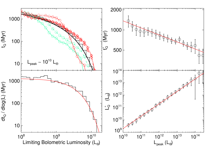
Figure 5.— Fits to the quasar lifetime as a function of luminosity from our simulations. Upper left shows the intrinsic, bolometric quasar lifetime $t_{Q}$ of a set of simulations with $L_{\rm peak}$ within a factor of 2 of $10^{10}\,L_{\sun}$, in the manner of Figure 4. The black histogram shows the geometric mean of these lifetimes, and the black histogram in the lower left shows the differential lifetime ${\rm d}t/{\rm d}\log{L}$ from this geometric mean. The black thick line in the upper left and red line in the lower left show the best-fit to our analytical form, ${\rm d}t/{\rm d}\log{L}=t^{\ast}_{Q}\,\exp(-L/L^{\ast}_{Q})$. Upper right shows the fitted $t^{\ast}_{Q}$ and resulting errors in each peak luminosity (final black hole mass) interval, and the best-fit power-law to $t^{\ast}_{Q}(L_{\rm peak})$ (red line). Lower right shows the fitted $L^{\ast}_{Q}$ and resulting errors in each peak luminosity (final black hole mass) interval, and the best-fit proportionality $L^{\ast}_{Q}\propto L_{\rm peak}$ (red line).

Although the truncated power-laws we have previously fitted to $t_{Q}$ using only the A-series simulations (Hopkins et al., 2005b) provide acceptable fits to all our runs, we use our new, larger set of simulations to improve the accuracy of the fits and average over peculiarities of individual simulations, giving a more robust prediction of the lifetime as a function of instantaneous and peak luminosity. For a given peak luminosity $L_{\rm peak}$, we consider simulations with an $L_{\rm peak}$ within a factor of 2, and take the geometric mean of their lifetimes $t_{Q}$($L$) (we ignore any points where $t_{Q}<1$ Myr, as our calculated lifetimes are uncertain below this limit). We can then differentiate this numerically to obtain ${\rm d}t/{\rm d}\log{L}$ (the time spent in a given logarithmic luminosity interval), and fit some functions to both curves simultaneously. Figure 5 illustrates this and shows the results of our fitting. We find that both the integrated lifetime $t_{Q}$($L$) and the differential lifetime ${\rm d}t/{\rm d}\log{L}$ are well fitted by an exponential,

$${\rm d}t/{\rm d}\log{L}=t^{\ast}_{Q}\,\exp[-L/L^{\ast}_{Q}],$$ (4)

where both $t^{\ast}_{Q}$ and $L^{\ast}_{Q}$ are functions of $M^{f}_{\rm BH}$ or $L_{\rm peak}$. The best-fit such ${\rm d}t/{\rm d}\log{L}$ is shown in the figure as a solid line for simulations with $L_{\rm peak}\sim 10^{10}\,L_{\sun}$, and agrees well with both the numerical derivative ${\rm d}t/{\rm d}\log{L}$ (lower left, black histogram) and the geometric mean $t_{Q}(L)$ (upper left, black histogram). This of course implies

$$t_{Q}(L)=t^{\ast}_{Q}\,\int^{L_{\rm peak}}_{L}e^{-L/L^{\ast}_{Q}}\,d\log{L},$$ (5)

but we are primarily interested in ${\rm d}t/{\rm d}\log{L}$ in our subsequent analysis.

Although our fitted lifetime involves an exponential, it is in no way similar to the exponential light curve of constant Eddington-ratio black hole growth or the model in, e.g., Haiman & Loeb (1998), which give ${\rm d}t/{\rm d}\log{L}=$ constant $\sim t_{S}\ll t^{\ast}_{Q}$.

Our functional form also has the advantage that, although it should formally be truncated with ${\rm d}t/{\rm d}\log{L}=0$ for $L>L_{\rm peak}$, the values in this regime fall off so quickly that we can safely use the above fit for all large $L$. Similarly, at $L\lesssim 10^{-4}\,L_{\rm peak}$, ${\rm d}t/{\rm d}\log{L}$ falls below the constant $t^{\ast}_{Q}$ to which this equation asymptotes. Furthermore, in this regime, the fits above begin to differ significantly from those obtained by fitting e.g. truncated power-laws or Schechter functions. However, these luminosities are well below those we generally consider and well below the luminosities where the contribution of a quasar with some $L_{\rm peak}$ is significant to the observed quantities we predict. Moreover, this turndown (i.e. the lower value predicted by an exponential as opposed to a power-law or Schechter function at low luminosities) is at least in part an artifact of the finite simulation duration. The values here are also significantly more uncertain, as by these low relative accretion rates, the system is likely to be accreting in some low-efficiency, ADAF state (e.g. Narayan & Yi 1995), which we do not implement directly in our simulations. Rather than introduce additional uncertainties into our modeling when they do not affect our predictions, we adopt these exponential fits which are accurate at $L\gtrsim 10^{-4}-10^{-3}\,L_{\rm peak}$. However, for purposes where the faint-end behavior of the quasar lifetime is important, such as predicting the value and evolution of the faint-end quasar luminosity function slope with redshift, a more detailed examination of the lifetime at low luminosities and relaxation of quasars after the “blowout” phase is necessary, and we consider these issues separately in Hopkins et al. (2005f).

We also note that in Hopkins et al. (2005c) we considered several extreme limits to our modeling, neglecting all times before the final merger and applying an ADAF correction at low accretion rates (taken into account a posteriori by rescaling the radiative efficiency $\epsilon_{r}$ with accretion rate, given the assumption that such low accretion rates do not have a large dynamical effect on the system regardless of radiative efficiency), and found that this does not change our results – the lifetime at low luminosities may be slightly altered but the key qualitative point, that the quasar lifetime increases with decreasing luminosity, is robust against a wide range of limits designed to decrease the lifetime at low luminosities.

Figure 5 further shows the fitted $t^{\ast}_{Q}$ (upper right) and $L^{\ast}_{Q}$ (lower right) as a function of peak quasar luminosity for each $L_{\rm peak}$. We find that $L^{\ast}_{Q}$, the luminosity above which the lifetime rapidly decreases, is proportional to $L_{\rm peak}$,

$$L^{\ast}_{Q}=\alpha_{L}L_{\rm peak},$$ (6)

with a best fit coefficient $\alpha_{L}=0.20$ (solid line). The weak dependence of $t^{\ast}_{Q}$ on $L_{\rm peak}$ is well-described by a power-law,

$$t^{\ast}_{Q}=t^{(10)}_{\ast}\,\Bigl{(}\frac{L_{\rm peak}}{10^{10}\,L_{\sun}}\Bigr{)}^{\alpha_{T}},$$ (7)

with $t^{(10)}_{\ast}=1.37\times 10^{9}\,{\rm yr}$ and $\alpha_{T}=-0.11$

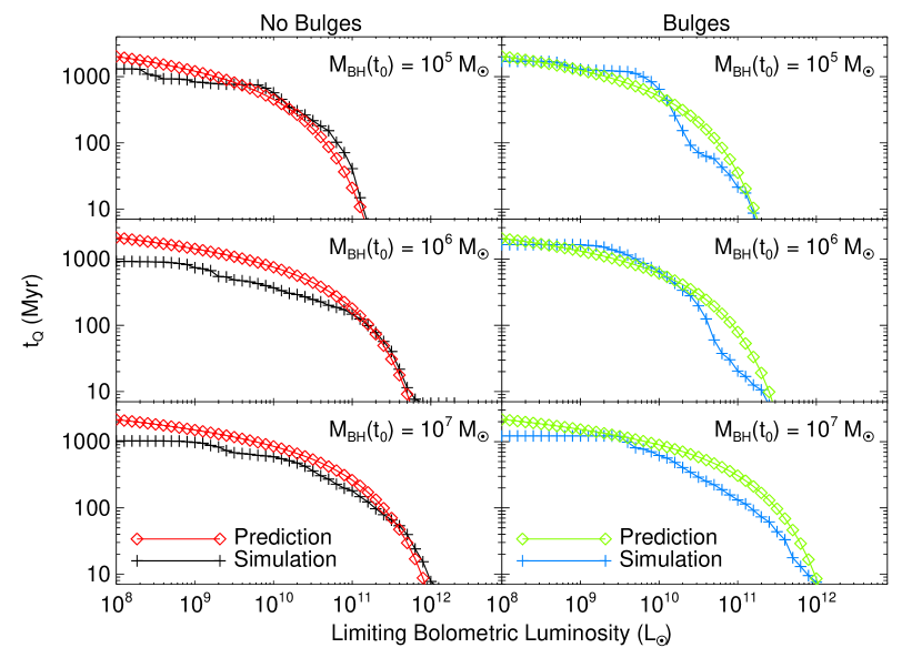
Figure 6.— Predicted quasar lifetime as a function of luminosity compared to that obtained in simulations with and without bulges and with different initial seed black hole masses. All simulations shown in this plot are initially identical to our fiducial A3 (Milky Way-like) case, but with or without an initial stellar bulge and with an initial seed black hole mass as labeled. Diamonds show the predicted quasar lifetime $t_{Q}$, a function of the peak luminosity of each simulated quasar, determined from the fits shown in Figure 5. Crosses show the lifetime determined directly in the simulations.

The presence or absence of a stellar bulge in the progenitors can have a significant impact on the quasar light curve (Springel et al. 2005b), primarily affecting the strength of the strong accretion phase associated with initial passage of the merging galaxies (e.g. Mihos & Hernquist 1994). Likewise, the seed mass of the simulation black holes could have an effect, as black holes with smaller initial masses will spend more time growing to large sizes, and more massive black holes may be able to shut down early phases of accretion in mergers in minor “blowout” events. In Figure 6, we show various tests to examine the robustness of our fitted quasar lifetimes to these variations. We have re-run our fiducial Milky Way-like A3 simulation both with (right panels) and without (left panels) initial stellar bulges in the merging galaxies and varying the initial black hole seed masses from $10^{4}-10^{7}\,M_{\sun}$. In each case we compare the lifetime $t_{Q}$ determined directly from the simulations (crosses) to that predicted from our fits above (diamonds), based only on the peak luminosity (final black hole mass) of the simulated quasar. Again, we find that varying these simulation parameters can have a significant effect on the final black hole mass, but that the quasar lifetime as a function of peak luminosity is a robust quantity, independent of initial black hole mass or the presence or absence of a bulge in the quasar host.

We can integrate the total radiative output of our model quasars,

$$E_{\rm rad}=\int^{L_{\rm peak}}_{L_{\rm min}}L\,\frac{{\rm d}t}{{\rm d}\log{L}}{\rm d}\log L,$$ (8)

and using our fitted formulae and $L_{\rm min}\ll L^{\ast}_{Q}$ we find

$$E_{\rm rad}=L^{\ast}_{Q}\,t^{\ast}_{Q}\,\log{e}\,(1-e^{-L_{\rm peak}/L^{\ast}_{Q}}).$$ (9)

Knowing $E_{\rm rad}=\epsilon_{r}M^{f}_{\rm BH}c^{2}$, we can compare the final black hole mass as a function of peak luminosity to what we would expect if the peak luminosity were the Eddington luminosity of a black hole with mass $M_{\rm Edd}$, $L_{\rm Edd}=\epsilon_{r}M_{\rm Edd}c^{2}/t_{S}$, where $t_{S}$ is the Salpeter time for $\epsilon_{r}=0.1$. Equating $E_{\rm rad}=\epsilon_{r}M^{f}_{\rm BH}c^{2}$ with the value calculated in Equation 9, and using the definition of the Eddington mass at $L=L_{\rm peak}$ and our fitted $L^{\ast}_{Q}=\alpha_{L}L_{\rm peak}$, we obtain

$$\frac{M^{f}_{\rm BH}(L_{\rm peak})}{M_{\rm Edd}(L_{\rm peak})}=\alpha_{L}\Bigl{(}\frac{t^{\ast}_{Q}}{t_{S}}\Bigr{)}\log e\approx 1.24\,f_{T},$$ (10)

where $f_{T}=(L_{\rm peak}/10^{13}\,L_{\sun})^{-0.11}$ for the power-law fit to $t^{\ast}_{Q}$. For our calculations explicitly involving black hole mass, we adopt this conversion unless otherwise noted, as we have performed our primary calculation (i.e. calculated $\dot{n}(L_{\rm peak})$) in terms of peak luminosity. Moreover, although this agrees well with the black hole masses in our simulations as a function of peak luminosity (as it must if the fitted quasar lifetimes are accurate), this allows us to smoothly interpolate to the highest black hole masses ($\sim{\rm a\ few}\,\times 10^{9}-10^{10}\,M_{\sun}$), which are of particular interest in examining the black hole population but for which the number of simulations we have with a given final black hole mass drops rapidly.

This gives explicitly the modifications to the black hole mass compared to that inferred from the “light bulb” and “constant Eddington ratio” models which we outline below in § 2.5, in which quasars shine at constant luminosity or follow exponential light curves, and for which $M_{\rm BH}^{f}=M_{\rm Edd}(L_{\rm peak})/l$, where $l$, the (constant) Eddington ratio, is generally adopted. The corrections are small, and therefore most of the black hole mass is accumulated in the bright, near-peak quasar phase, in good agreement with observational estimates (e.g., Soltan, 1982; Yu & Tremaine, 2002); we discuss this in greater detail in § 4 and § 6. Furthermore, the increase of $f_{T}$ with decreasing $L_{\rm peak}$ implies that lower-mass quasars accumulate a larger fraction of their mass in slower, sub-peak accretion after the final merger, while high-mass objects acquire essentially all their mass in the peak quasar phase. This is seen directly in our simulations, and is qualitatively in good agreement with expectations from simulations and semi-analytical models in which the $M_{\rm BH}-\sigma$ relation is set by black hole feedback in a strong quasar phase. Compared to the assumption that $M_{BH}^{f}=M_{\rm Edd}(L_{\rm peak})$, this formula introduces a small but non-trivial correction in the relic supermassive black hole mass function implied by the quasar luminosity function and $\dot{n}(L_{\rm peak})$ (see § 6).

The predictions of our model for the quasar lifetime and evolution can be applied to observations which attempt to constrain the quasar lifetime from individual quasars, for example using the proximity effect in the Ly$\alpha$ forest (Bajtlik, Duncan, & Ostriker, 1988; Haiman & Cen, 2002; Jakobsen et al., 2003; Yu & Lu, 2005) and multi-epoch observations (Martini & Schneider, 2003). However, many observations designed to constrain the quasar lifetime do so not for individual quasars, but using demographic or integral arguments based on the population of quasars in some luminosity interval (e.g., Soltan, 1982; Haehnelt, Natarajan, & Rees, 1998; Yu & Tremaine, 2002; Yu & Lu, 2004; Porciani, Magliocchetti, & Norberg, 2004; Grazian et al., 2004). Our prediction for these observations is similar but slightly more complex, as an observed luminosity function at a given luminosity will consist of sources with different peak luminosities $L_{\rm peak}$, but the same instantaneous luminosity, $L$. Furthermore, the lifetime being probed may be either the integrated quasar lifetime above some luminosity threshold or the differential lifetime at a particular luminosity.

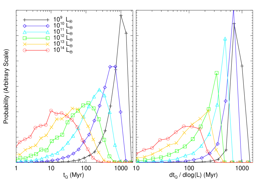
Figure 7.— Predicted distribution (fractional number density per logarithmic interval in lifetime) of quasar lifetimes at different bolometric luminosities, for the luminosity function determined in § 3 at $z=0.5$. Left panel plots the distribution of integrated lifetimes $t_{Q}$ (time spent over the course of each quasar lifetime above the given luminosity). Right panel plots the distribution of differential lifetimes ${\rm d}t/{\rm d}\log{L}$ (time spent by each quasar in a logarithmic interval about the given luminosity).

For a given determination of the quasar luminosity function using our model for quasar lifetimes and some distribution of peak luminosities, we can predict the distribution of quasar lifetimes as a function of the observed luminosity interval. Figure 7 shows an example of such a result, using the determination of the luminosity function below in § 3.2, at redshift $z=0.5$. We consider several bolometric luminosities spanning the luminosity function from $10^{9}-10^{14}\,L_{\sun}$, and for each, the distribution of sources (peak luminosities), and the corresponding distribution of quasar lifetimes. We show both the distribution of integrated quasar lifetimes $t_{Q}$ (left panel) and the distribution of differential quasar lifetimes ${\rm d}t/{\rm d}\log{L}$ (right panel). The evolution with redshift is weak, with the lifetime increasing by $\sim 1.5-2$ at a given luminosity at $z=2$. There is furthermore an ambiguity of a factor $\sim 2$, as some of the quasars observed at a given luminosity will only be entering a peak quasar phase, whereas the lifetimes shown are integrated over the whole quasar evolution. This prediction is quite different from that of the optical quasar phase which we describe below in § 4 and in Hopkins et al. (2005a), as it considers only the intrinsic bolometric luminosity, but our modeling and the fits provided above for the bolometric lifetime and column density distributions should enable the prediction of these quantities, considering attenuation, in any waveband. In either case, it is clear that the lifetime distribution for lower-luminosity quasars is increasingly more strongly peaked and centered around longer lifetimes, in good agreement with the limited observational evidence from e.g. Adelberger & Steidel (2005). This is a consequence of the fact that in our model quasar lifetimes decrease with increasing luminosity. The range spanned in the figure corresponds well to the range of quasar lifetimes implied by the observations above and others (e.g. Martini, 2004, and references therein).

2.5. Alternative Models of Quasar Evolution

Our modeling reproduces at least the observed hard X-ray quasar luminosity function by construction, since we use the observed quasar luminosity functions to determine the birthrate of quasars of a given $L_{\rm peak}$, $\dot{n}(L_{\rm peak})$, in § 3.2. It is therefore useful to consider in detail the differences in our subsequent predictions between various models for the quasar lifetime and obscuration, in order to determine to what extent these predictions are implied by any model that successfully reproduces the observed quasar luminosity function, and to what extent they are independent of the observed luminosity functions and instead depend on the model of quasar evolution adopted. To this end, we define two models for the quasar lifetime, and two models for the distribution of quasar column densities, combinations of which have been commonly used in most previous analyses of quasars.

For the quasar lifetime, we consider the following two cases:

“Light-Bulb Model” (e.g., Small & Blandford, 1992; Kauffmann & Haehnelt, 2000; Wyithe & Loeb, 2003; Haiman, Quataert, & Bower, 2004). The simplest possible model for the quasar light curve, the “feast or famine” or “light-bulb” model assumes that quasars have only two states, “on” and “off.” Quasars turn “on”, shine at a fixed bolometric luminosity $L=L_{\rm peak}$, defined by a “constant” Eddington ratio (i.e. $L_{\rm peak}=l\,M_{\rm BH}^{f}$) and constant quasar lifetime $t_{Q,\,\rm LB}$. Models where quasars live arbitrarily long with slowly evolving mean volume emissivity or mean light curve (e.g. Small & Blandford, 1992; Haiman & Menou, 2000; Kauffmann & Haehnelt, 2000) are equivalent to the “light bulb” scenario, as they still assume that quasars observed at a luminosity $L$ radiate at that approximately constant luminosity over some universal lifetime $t_{Q,\,\rm LB}$ at a particular redshift. We adopt $l=0.3$ and $t_{Q,\,\rm LB}=10^{7}\,$yr, as is commonly assumed in theoretical work and suggested by observations (given this prior) (e.g. Yu & Tremaine, 2002; Martini, 2004; Soltan, 1982; Yu & Lu, 2004; Porciani, Magliocchetti, & Norberg, 2004; Grazian et al., 2004), and similar to the $e$-folding time of a black hole with canonical radiative efficiency $\epsilon_{r}=0.1$ (Salpeter, 1964) or the dynamical time in a typical galactic disk or central regions of the merger. These choices control only the normalization of $\dot{n}(L_{\rm peak})$, and therefore do not affect most of our predictions. Where the normalization (i.e. value of the constant $t_{Q}$ or $l$) is important, we allow it to vary in order to produce the best possible fit to the observations.

“Exponential (Fixed Eddington Ratio) Model.” A somewhat more physical model of the quasar light curve is obtained by assuming growth at a constant Eddington ratio, as is commonly adopted in e.g. semi-analytical models which attempt to reproduce quasar luminosity functions (e.g. Kauffmann & Haehnelt, 2000; Wyithe & Loeb, 2003; Volonteri et al., 2003). In this model, a black hole accretes at a fixed Eddington ratio $l$ from an initial mass $M_{i}$ to a final mass $M_{f}$ (or equivalently, a final luminosity $L_{f}=l\,L_{Edd}(M_{f})$), and then shuts off. This gives exponential mass and luminosity growth, and the time spent in any logarithmic luminosity bin is constant,

$$dt/{\rm d}\log(L)=t_{S}\,(\ln(10)/l)$$ (11)

for $L_{i}<L<L_{f}$. This is true for any exponential light curve; i.e. this model includes cases with an exponential decline in quasar luminosity), $f(t)\propto e^{\pm t/t_{\ast}}$, such as that of Haiman & Loeb (1998), with only the normalization $dt/{\rm d}\log(L)=t_{\ast}\,\ln(10)$ changed, and thus any such model will give identical results with correspondingly different normalizations. As with the “light-bulb” model, we are free to choose the characteristic Eddington ratio and corresponding timescale for this lightcurve, and we adopt $l=0.3$ (i.e. $t_{\ast}\sim 10^{8}\,$yr) in general. Again, however, we allow the normalization to vary freely where it is important, such that these models have the best chance to reproduce the observations. For our purposes, models in which this timescale is determined by e.g. the galaxy dynamical time and thus are somewhat dependent on host galaxy mass or redshift are nearly identical to this scenario. Further, insofar as the dynamical time increases weakly with increasing host galaxy mass (as, e.g. for a spheroid with $M_{\rm BH}\propto M_{\rm vir}\sim a\,\sigma^{2}/G$, where $a$ is the spheroid scale length and $M_{\rm BH}\propto\sigma^{4}$, such that $t_{\rm dyn}\sim a/\sigma\propto\sigma\propto M_{\rm vir}^{1/4}$), this produces behavior qualitatively opposite to our predictions (of increasing lifetime with decreasing instantaneous luminosity), and yields results which are even more discrepant from our predictions and the observations than the constant (host-galaxy independent) case.

A wide variety of “light-bulb” or exponential (constant Eddington ratio) models are possible, allowing for different distributions of typical Eddington ratios and/or quasar lifetimes (see e.g. Steed & Weinberg 2003 for an extensive comparison of several classes of such models), but for our purposes they are essentially identical insofar as they do not capture the essential qualitative features of our quasar lifetimes, namely that the quasar lifetime depends on both instantaneous and peak luminosities, and increases with decreasing instantaneous luminosity.

We fit both of the simple models above to the observed quasar luminosity functions in the same manner described in § 3, (i.e. in the same manner as we fit our more complicated models of quasar evolution), to determine $\dot{n}(L_{\rm peak})_{\rm LB}$ for the “light-bulb” model and $\dot{n}(L_{\rm peak})_{\rm Edd}$ for the “fixed Eddington ratio” model (see Equations 15 and 16, respectively). Thus all three models of the quasar light curve, the “light-bulb”, “fixed Eddington ratio”, and our luminosity-dependent lifetimes model produce an essentially identical bolometric luminosity function.

We also consider two commonly adopted alternative models for the column density distribution and quasar obscuration:

“Standard (Luminosity-Independent) Torus” (e.g. Antonucci, 1993). This is the canonical obscuration model, based on observations of local, low-luminosity Seyfert galaxies (e.g., Risaliti et al., 1999). The column density distribution is derived from the torus geometry, where we assume the torus inner radius lies at a distance $R_{\rm T}$ from the black hole, with a height $H_{\rm T}$, and a density distribution $\rho(\theta)\propto\exp(-\gamma|\cos\theta|)$, where $\theta$ is the polar angle and the torus lies in the $\theta=0$ plane. This results in a column density as a function of viewing angle of

$$N_{\rm H}(\theta) = N_{\rm H,\,0}\,\exp(-\gamma|\cos\theta|)\,\cos(90-\theta)\,$$ (12)

$$\times\sqrt{\Bigl{(}\frac{R_{\rm T}}{H_{\rm T}}\Bigr{)}^{2}-\sec^{2}(90-\theta)\Bigl{(}\Bigl{(}\frac{R_{\rm T}}{H_{\rm T}}\Bigr{)}^{2}-1\Bigr{)}}$$

(Treister et al., 2004). Here, $N_{\rm H,\,0}$ is the column density along a line of sight through the torus in the equatorial plane and $\gamma$ parameterizes the exponential decay of density with viewing angle. This is a phenomenological model, and as a result the parameters are essentially all free. We adopt typical values, an equatorial column density $N_{\rm H,\,0}=10^{24}$ cm^-2, radius-to-height ratio $R_{\rm T}/H_{\rm T}=1.1$, and density profile $\gamma=4$. This combination of parameters follows Treister et al. (2004), and is designed to fit the observed X-ray column density distribution and give a ratio of obscured to unobscured quasars $\sim 3$, similar to the mean locally observed value (e.g. Risaliti et al., 1999).

“Receding (Luminosity-Dependent) Torus” (e.g. Lawrence, 1991). Many observations suggest that the fraction of obscured objects depends on luminosity (Steffen et al., 2003; Ueda et al., 2003; Hasinger, 2004; Grimes, Rawlings, & Willott, 2004; Sazonov & Revnivtsev, 2004; Barger et al., 2005; Simpson, 2005). Therefore, some theoretical works have adopted a “receding torus” model, in which the torus radius $R_{\rm T}$ (i.e. distance from the quasar) is allowed to vary with luminosity, but the height and other parameters remain constant. The torus radius is assumed to increase with luminosity, enlarging the opening angle and thus the fraction of unobscured quasars. In this case, the column densities are identical to those shown above, but now $R_{\rm T}/H_{\rm T}=(L/L_{0})^{0.5}$, where $L_{0}\approx 10^{11}\,L_{\sun}$ is the luminosity at which the ratio of obscured to unobscured quasars is $\approx 3:1$ and the power-law slope is chosen to fit the dependence of obscured fraction on luminosity.

Both of these column density distributions represent phenomenological models with several free parameters, explicitly chosen to reproduce the observed differences in quasar luminosity functions and column density distributions. Despite this, it is not clear that these functional forms represent the best possible fit to the observations they are designed to reproduce. Furthermore, comparison of our results in which column density distributions depend on luminosity and peak luminosity elucidates the importance of proper modeling of the dependence of column density on quasar evolution.

3. The Quasar Luminosity Function

3.1. The Effect of Luminosity-Dependent Quasar Lifetimes

Given quasar lifetimes as functions of both instantaneous and peak luminosities, the observed quasar luminosity function (in the absence of selection effects) is a convolution of the lifetime with the intrinsic distribution of sources with a given $L_{\rm peak}$. If sources of a given $L$ are created at a rate $\dot{n}(L,t)$ (per unit comoving volume) at cosmological time $t_{H}\sim 1/H(z)$ and live for some lifetime $\Delta t_{Q}(L)$, the total comoving number density observed will be

$$\Delta n=\int^{t_{H}+\Delta t_{Q}(L)}_{t_{H}}\dot{n}(L,t)\,{\rm d}t,$$ (13)

which, for a cosmologically evolving $\dot{n}(L,t)$, can be expanded about $\dot{n}(L,t_{H})$, yielding $\Delta n=\dot{n}(L,t_{H})\,\Delta t_{Q}(L)$ to first order in $\Delta t_{Q}(L)/t_{H}$. Considering a complete distribution of sources with some $L_{\rm peak}$, we similarly obtain the luminosity function

$$\phi(L)\equiv\frac{{\rm d}\Phi}{{\rm d}\log L}(L)=\int{\frac{{\rm d}t(L,L_{\rm peak})}{{\rm d}\log(L)}\,\dot{n}(L_{\rm peak})}\,{\rm d}\log(L_{\rm peak}).$$ (14)

Throughout, we will denote the differential luminosity function, i.e. the comoving number density of quasars in some logarithmic luminosity interval, as $\phi\equiv{\rm d}\Phi/{\rm d}\log L$. Here, $\dot{n}(L_{\rm peak})$ is the comoving number density of sources created per unit cosmological time per logarithmic interval in $L_{\rm peak}$, at some redshift, and ${\rm d}t/{\rm d}\log{L}$ is the differential quasar lifetime, i.e. the total time that a quasar with a given $L_{\rm peak}$ spends in a logarithmic interval in bolometric luminosity $L$. This formulation implicitly accounts for the “duty cycle” (the fraction of active quasars at a given time), which is proportional to the lifetime at a given luminosity. Corrections to this formula owing to finite lifetimes are of order $({\rm d}t/{\rm d}\log{L})/t_{H}$, which for the luminosities and redshifts considered here (except for Figure 11), are never larger than $\sim 1/5$ and are generally $\ll 1$, which is significantly smaller than the uncertainty in the luminosity function itself.

We next consider the implications of our luminosity-dependent quasar lifetimes for the relation between the observed luminosity function and the distribution of peak luminosities (i.e. intrinsic properties of quasar systems). In traditional models of quasar lifetimes and light curves, this relation is trivial. For example, models in which quasars “turn on” at fixed luminosity for some fixed lifetime (i.e. the “light-bulb” model defined in § 2.5) imply

$$\dot{n}(L_{\rm peak})_{\rm LB}\propto\phi(L=L_{\rm peak}),$$ (15)

and models in which quasar light curves are a pure exponential growth or decay with some cutoff(s) (e.g., exponential or fixed Eddington-ratio models) imply

$$\dot{n}(L_{\rm peak})_{\rm Edd}\propto\frac{d\phi}{{\rm d}\log(L)}\raisebox{-3.0pt}{\huge$\mid$}_{L=L_{\rm peak}}.$$ (16)

These both have essentially identical shape to the observed luminosity function, qualitatively different from our model prediction that $\dot{n}(L_{\rm peak})$ should turn over at luminosities approximately below the break in the observed luminosity function (see, e.g. Fig. 1 of Hopkins et al. 2005e). The luminosity-dependent quasar lifetimes determined from our simulations imply a new interpretation of the luminosity function, with $\dot{n}(L_{\rm peak})$ tracing the bright end of the luminosity function similar to traditional models, but then peaking and turning over below $L_{\rm peak}\sim L_{\rm break}$, the break luminosity in standard double power-law luminosity functions. In our deconvolution of the luminosity function, the faint end corresponds primarily to sources in sub-Eddington phases transitioning into or out of the phase(s) of peak quasar activity. There is also some contribution to the faint-end lifetime from quasars accreting efficiently (i.e. growing exponentially at high Eddington ratio) early in their activity and on their way to becoming brighter sources, but this becomes an increasingly small fraction of the lifetime at lower luminosities. For example, in Figure 7 of Hopkins et al. (2005b), direct calculation of the quasar lifetime shows that sub-Eddington phases begin to dominate the lifetime for $L\lesssim 0.1\,L_{\rm peak}$, with $\gtrsim 90\%$ of the lifetime at $L\sim 10^{-3}\,L_{\rm peak}$ corresponding to sub-Eddington growth. By definition, a “fixed Eddington ratio” or “light bulb” model is dominated at all luminosities by a fixed, usually large, Eddington ratio. Even models which assume an exponential decline in the quasar luminosity from some peak, although they clearly must spend a significant amount of time at low Eddington ratios, have an identical $\dot{n}(L_{\rm peak})=\dot{n}(L_{\rm peak})_{\rm Edd}$ (modulo an arbitrary normalization), and predict far less time at most observable ($\gtrsim 10^{-4}\,L_{\rm peak}$) low luminosities and accretion rates (because the accretion rates fall off so rapidly); i.e. the population at any observed luminosity is still dominated by objects near their peak.

Figure 8.— We reproduce (thin histogram) the luminosity function of Ueda et al. (2003) at redshift $z=0.5$ (thin curve) using the binned differential quasar lifetime ${\rm d}t/{\rm d}\log{L}$ directly from our simulations and a fitted distribution of peak luminosities $\dot{n}(L_{\rm peak})$ (thick histogram). For each bin in $\log(L_{\rm peak})$, we average the binned differential lifetime of a set of simulations with peak luminosity in the bin. This clearly demonstrates our key qualitative result, that the faint end of the luminosity function is reproduced by quasars with peak luminosity around the break luminosity but observed primarily in sub-Eddington states (luminosities $L\ll L_{\rm peak}$), is not an artifact of our fitting formulae or extrapolation to extreme luminosities.

From our new, large set of simulations, we test this model of the relationship between the distribution of peak quasar luminosities and observed luminosity functions, namely our assertion that $\dot{n}(L_{\rm peak})$ should peak around the observed break in the luminosity function, and turn over below this peak, with the observed luminosity function faint-end slope dominated by sources with peak luminosities near the break in sub-Eddington (sub-peak luminosity) states. In particular, we wish to ensure that this behavior for $\dot{n}(L_{\rm peak})$ is real, and not some artifact of our fitting functions for the quasar lifetime.

Figure 8 shows the best fit $\dot{n}(L_{\rm peak})$ distribution (solid thick histogram) fitted to the Ueda et al. (2003) hard X-ray quasar luminosity function (solid curve) at redshift $z=0.5$, as well as the resulting best-fit luminosity function (solid thin histogram). For ease of comparison with other quasar luminosities, we rescale the luminosity function to the bolometric luminosity using the corrections of Marconi et al. (2004). We determine $\dot{n}(L_{\rm peak})$ by logarithmically binning the range of $L_{\rm peak}$, and considering for each bin all simulations with $L_{\rm peak}$ in the given range. For each bin, then, we take the average binned time the simulations spend in each luminosity interval, and take that to be the quasar lifetime ${\rm d}t/{\rm d}\log{L}$. We then fit to the observed luminosity function of Ueda et al. (2003), fitting

$$\phi(L)\approx\sum_{i}\ \dot{n}_{i}(L_{{\rm peak},\,i})\,{\left\langle{\frac{\Delta t(L,\,L_{{\rm peak},\,i})}{\Delta\log L}}\right\rangle}$$ (17)

and allowing $\dot{n}_{i}(L_{{\rm peak},\,i})$ to be a free coefficient for each binned $L_{\rm peak}=L_{{\rm peak},\,i}$. Despite our large number of simulations, the numerical binning process makes this result noisy, especially at the extreme ends of the luminosity function. However, the relevant result is clear – the qualitative behavior of $\dot{n}(L_{\rm peak})$ described above is unchanged. For further discussion of the qualitative differences between the $\dot{n}(L_{\rm peak})$ distribution from different quasar models, and the robust nature of our interpretation even under restrictive assumptions (e.g. ignoring the early phases of merger activity or applying various models for radiative efficiency as a function of accretion rate), we refer to Hopkins et al. (2005c).

3.2. The Luminosity Function at Different Frequencies and Redshifts

Given a distribution of peak luminosities $\dot{n}(L_{\rm peak})$, we can use our model of quasar lifetimes and the column density distribution as a function of instantaneous and peak luminosities to predict the luminosity function at any frequency. From a distribution of $N_{\rm H}$ values and some a priori known minimum observed luminosity $L_{\nu}^{\rm min}$, the fraction $f_{\rm obs}$ of quasars with a peak luminosity $L_{\rm peak}$ and instantaneous bolometric luminosity $L$ which lie above the luminosity threshold is given by the fraction of $N_{\rm H}$ values below a critical $N_{H}^{\rm max}$, where $L_{\nu}^{\rm min}=f_{\nu}L\,\exp{(-\sigma_{\nu}N_{H}^{\rm max})}$. Here, $f_{\nu}(L)\equiv L_{\nu}/L$ is a bolometric correction and $\sigma_{\nu}$ is the cross-section at frequency $\nu$. Thus,

$$N_{H}^{\rm max}(\nu,L,L_{\nu}^{\rm min})=\frac{1}{\sigma_{\nu}}\ln{\Bigl{(}\frac{f_{\nu}(L)L}{L_{\nu}^{\rm min}}\Bigr{)}},$$ (18)

and for the lognormal distribution above,

$$f_{\rm obs}(\nu,L,L_{\rm peak},L_{\nu}^{\rm min})=\frac{1}{2}\Bigl{[}1+{\rm erf}\Bigl{(}\frac{\log{(N_{H}^{\rm max}/\bar{N}_{H})}}{\sqrt{2}\,\sigma_{N_{H}}}\Bigr{)}\Bigr{]}.$$ (19)

This results in a luminosity function (in terms of the bolometric luminosity)

$$\phi(\nu,L,L_{\nu}^{\rm min}) = \int{f_{\rm obs}(\nu,L,L_{\rm peak},L_{\nu}^{\rm min})}$$ (20)

$$\quad\times\frac{dt(L,L_{\rm peak})}{{\rm d}\log(L)}\,\dot{n}(L_{\rm peak})\,d\log(L_{\rm peak}),$$

where $\phi(\nu,L,L_{\nu}^{\rm min})$ is the number density of sources with bolometric luminosity $L$ per logarithmic interval in $L$, with an observed luminosity at frequency $\nu$ above $L_{\nu}^{\rm min}$.

Based on the direct fit for $\dot{n}(L_{\rm peak})$ in Figure 8, we wish to consider a functional form for $\dot{n}(L_{\rm peak})$ with a well-defined peak and falloff in either direction in $\log(L_{\rm peak})$. Therefore, we take $\dot{n}(L_{\rm peak})$ to be a lognormal distribution, with

$$\dot{n}(L_{\rm peak})=\dot{n}_{\ast}\ \frac{1}{\sigma_{\ast}\sqrt{2\pi}}\exp\Bigl{[}-\frac{1}{2}\,\Bigl{(}\frac{\log(L_{\rm peak}/L_{\ast})}{\sigma_{\ast}}\Bigr{)}^{2}\Bigr{]}.$$ (21)

Here, $\dot{n}_{\ast}$ is the total number of quasars being created or activated per unit comoving volume per unit time; $L_{\ast}$ is the center of the lognormal, the characteristic peak luminosity of quasars being born (i.e. the peak luminosity at which $\dot{n}(L_{\rm peak})$ itself peaks), which is directly related to the break luminosity in the observed luminosity function; and $\sigma_{\ast}$ is the width of the lognormal in $\dot{n}(L_{\rm peak})$, and determines the slope of the bright end of the luminosity function. Since our model predicts that the bright end of the luminosity function is made up primarily of sources at high Eddington ratio near their peak luminosity, i.e. essentially identical to “light-bulb” or “fixed Eddington ratio” models, the bright-end slope is a fitted quantity, determined by whatever physical processes regulate the bright-end slope of the active black hole mass function (possibly feedback from outflows or threshold cooling processes, e.g. Wyithe & Loeb 2003; Scannapieco & Oh 2004; Dekel & Birnboim 2004), unlike the faint-end slope which is a consequence of the quasar lifetime itself, and is only weakly dependent on the underlying faint-end active black hole mass or $\dot{n}(L_{\rm peak})$ distribution.

We note that although this choice of fitting function has appropriate general qualities, it is ultimately somewhat arbitrary, and we choose it primarily for its simplicity and its capacity to match the data with a minimum of free parameters. We could instead, for example, have chosen a double power-law form with $\dot{n}(L_{\rm peak})=\dot{n}_{\ast}/[(L_{\rm peak}/L_{\ast})^{\gamma_{1}}+(L_{\rm peak}/L_{\ast})^{\gamma_{2}}]$ and $\gamma_{1}<\gamma_{2}$, but given that the entire faint end of the luminosity function is dominated by objects with $L_{\rm peak}\sim L_{\ast}$, the observed luminosity function has essentially no power to constrain the faint end slope $\gamma_{1}$, other than setting an upper limit $\gamma_{1}\lesssim 0$. The “true” $\dot{n}(L_{\rm peak})$ will, of course, be a complicated function of both halo merger rates at a given redshift and the distribution of host galaxy properties including, but not necessarily limited to, masses, concentrations, and gas fractions.

Having chosen a form for $\dot{n}(L_{\rm peak})$, we can then fit to an observed luminosity function to determine $(\dot{n}_{\ast},\,L_{\ast},\,\sigma_{\ast})$. We take advantage of the capability of our model to predict the luminosity function at multiple frequencies, and consider both fits to just the Ueda et al. (2003) hard X-ray (2-10 keV) luminosity function, $\phi_{HX}$, and fits to the Ueda et al. (2003), Miyaji et al. (2001) soft X-ray (0.5-2 keV; $\phi_{SX}$), and Croom et al. (2004) optical B-band (4400 Å; $\phi_{B}$) luminosity functions simultaneously. These observations agree with other, more recent determinations of $\phi_{HX},\ \phi_{SX},\ \phi_{B}$ (e.g. Barger et al., 2005; Hasinger, Miyaji, & Schmidt, 2005; Richards et al., 2005, respectively) at most luminosities, and therefore we do not expect revisions to the observed luminosity functions to dramatically change our results. In order to avoid numerical artifacts from fitting to extrapolated, low-luminosity slopes in the analytical forms of these luminosity functions, we directly fit to the binned luminosity function data. Thus, we fit each luminosity function in all redshift intervals for which we have binned data.

We find good fits ($\chi^{2}/\nu=68.8/104\approx 0.66$) to all luminosity functions at all redshifts with a pure peak-luminosity evolution (PPLE) model, for which

$$L_{\ast}=L_{\ast}^{0}\,\exp({k_{L}\,\tau}),\ \dot{n}_{\ast}=constant,\ \sigma_{\ast}=constant,$$ (22)

where $\tau$ is the fractional lookback time ($\tau\equiv H_{0}\int^{z}_{0}dt$) and $k_{L}$ is a dimensionless constant fitted with $L_{\ast},\,\dot{n}_{\ast},\,\sigma_{\ast}$. It is important to distinguish this from “standard” pure luminosity evolution (PLE) models (e.g., Boyle et al., 1988), as with $\dot{n}(L_{\rm peak})>0$ and $L_{\ast}=L_{\ast}(z)$ always, the density of sources, especially as a function of observed luminosity at some frequency, evolves in a non-trivial manner.

We do not find significant improvement in the fits if we additionally allow $\dot{n}_{\ast}$ or $\sigma_{\ast}$ to evolve with redshift ($\Delta\chi^{2}\sim 1-2$, depending on the adopted form for the evolution), and therefore consider only the simplest parameterization above (Equation 22). We also find acceptable fits for a pure density evolution model, with $L_{\ast}=$ constant and $\dot{n}_{\ast}=\dot{n}_{\ast}^{0}\,\exp{(k_{N}\,\tau)}$ (both keeping $\sigma_{\ast}$ fixed and allowing it to evolve as well). However, the fits are somewhat poorer ($\chi^{2}/\nu\approx 1$), and the resulting parameters over-produce the present-day density of low-mass supermassive black holes and the intensity of the X-ray background by an order of magnitude, so we do not consider them further. In either case, there is a considerable degeneracy between the parameters $\sigma_{\ast}$ and $L_{\ast}$, where a decrease in $L_{\ast}$ can be compensated by a corresponding increase in $\sigma_{\ast}$. This degeneracy is present because, as indicated above, the observed luminosity function only weakly constrains the faint-end slope of $\dot{n}(L_{\rm peak})$.

The observations shown are insufficient at high redshift to strongly resolve the “turnover” in the total comoving quasar density at $z\sim 2-3$, and thus we acknowledge that there must be corrections to this fitted evolution at higher redshift, which we address below. However, as we primarily consider low redshifts, $z\lesssim 3$, and show that the supermassive black hole population and X-ray background are dominated by quasars at redshifts for which our $\dot{n}(L_{\rm peak})$ distribution is well determined, this is not a significant source of error in most of our calculations even if we extrapolate our evolution to $z\gg 3$.

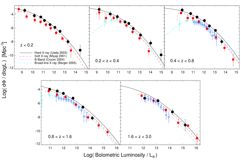
Figure 9.— Best-fit luminosity function from the pure peak-luminosity evolution $\dot{n}(L_{\rm peak})$ distribution, for redshifts $z=0-3$. From our fitted lognormal $\dot{n}(L_{\rm peak})$ distribution, we simultaneously reproduce the luminosity function in the hard X-ray (2-10 keV; solid black line), soft X-ray (0.5-2 keV; dashed red line), and optical B-band (4400 Å; dotted blue line) at all redshifts. Moreover, we reproduce the distribution of broad-line quasars in hard X-ray selected samples (cyan dot-dashed line), as described in § 4. All quantities have been rescaled to bolometric luminosities for ease of comparison, using the corrections of Marconi et al. (2004), with the plotted error bars representing both quoted measurement errors and the estimated errors in the bolometric corrections. The observations are from Miyaji et al. (2001) (soft X-ray; red squares), Ueda et al. (2003) (hard X-ray; black circles), Croom et al. (2004) (B-band, blue diamonds), and Barger et al. (2005) (X-ray selected broad-line quasars; cyan crosses).

Figure 9 shows the resulting best-fit PPLE luminosity functions from the best-fit $\dot{n}(L_{\rm peak})$ distribution, for redshifts $z=0-3$. This has the best-fit ($\chi^{2}/\nu=0.67$) values $(\log L_{\ast},k_{L},\,\log\dot{n}_{\ast},\,\sigma_{\ast})=(9.94,\,5.61,\,-6.29,\,0.91)$ with corresponding errors $(0.29,0.28,0.13,0.09)$. Here, $L_{\ast}$ is in solar luminosities and $\dot{n}_{\ast}$ in comoving ${\rm Mpc^{-3}\,Myr^{-1}}$. Fitting to the hard X-ray data alone gives a similar fit, with the slightly different values $(\log L_{\ast},k_{L},\,\log\dot{n}_{\ast},\,\sigma_{\ast})=(9.54,\,4.90,\,-5.86,\,1.03)\pm(0.66,0.43,0.37,0.13)$, $\chi^{2}/\nu=0.7$ (note the degeneracy between $L_{\ast}$ and $\sigma_{\ast}$ in the two fits). Our best-fit value of $k_{L}=5.6$ compares favorably to the value $\sim 6$ found by e.g. Boyle et al. (2000) and Croom et al. (2004) for the evolution of the break luminosity in the observed luminosity function, demonstrating that the break luminosity traces the peak in the $\dot{n}(L_{\rm peak})$ distribution at all redshifts. These fits and the errors were obtained by least-squares minimization over all data points (comparing each to the predicted curve at its redshift and luminosity), assuming the functional form we have adopted for $\dot{n}(L_{\rm peak})$.

The agreement we obtain at all redshifts, in each of the hard X-ray (black solid line), soft X-ray (red dashed line), and B-band (dark blue dotted line) is good. This is not at all guaranteed by our procedure, as the fit is highly over-constrained, because we fit three luminosity functions each at five redshifts to only four free parameters. Of course, the choice of the functional form for $\dot{n}(L_{\rm peak})$ ensures that we should be able to reproduce at least one luminosity function and its evolution (e.g. the hard X-ray luminosity function, which is least affected by attenuation), but our modeling of the column density distributions in mergers allows us to simultaneously reproduce the luminosity functions in different wavebands without imposing assumptions about obscured fractions or sources of attenuation. Expressed as bolometric luminosity functions, $\phi_{B}$, $\phi_{SX}$, and $\phi_{HX}$ would be identical in the absence of obscuration, similar to the predicted $\phi_{HX}$ as obscuration is minimal in the hard X-ray.

Figure 10.— Hard X-ray (thick), soft X-ray (thin), and B-band (dot-dash) LFs determined from our model of quasar lifetimes and column densities, based on a distribution of intrinsic source properties fitted to the observed hard X-ray LF and the limiting magnitudes of observed samples, at the different redshifts shown. All quantities are rescaled to bolometric luminosities with the bolometric corrections of Marconi et al. (2004). Symbols show the observed LFs for hard X-rays (Ueda et al., 2003, diamonds), soft X-rays (Miyaji et al., 2000, triangles), and B-band (Boyle et al., 2000, crosses). Reproduced from Hopkins et al. (2005d).

For redshifts $z\leq 1$, we reproduce in our Figure 10, Fig. 2 of Hopkins et al. (2005d), which shows in detail the agreement between hard X-ray (Ueda et al., 2003), soft X-ray (Miyaji et al., 2000), and optical (Boyle et al., 2000) luminosity functions resulting from the time and luminosity dependent column density distributions derived from the simulations. The differential extinction predicted for different frequencies (and magnitude limits) of observed samples based on the column density distributions in our simulations accounts for the different shape of the luminosity function in each band, and the evolution of the luminosity function with redshift is driven by a changing $L_{\ast}$, the peak of the $\dot{n}(L_{\rm peak})$ distribution (Equation 22). We emphasize that in our analysis, the key quantity constrained by observations is the fitted $\dot{n}(L_{\rm peak})$ distribution with redshift. All other quantities and distributions are derived from the basic input physics of our simulations, with no further assumptions or adjustable factors in our modeling beyond the prescription for Bondi (Eddington-limited) accretion and $\sim 5\%$ energy deposition in the ISM, which are themselves constrained by observations and theory as discussed in § 2 and in Di Matteo et al. (2005).

We can, of course, fit the previously defined simpler model of quasar lifetimes, either a “light-bulb” or exponential light curve/fixed Eddington ratio model, and obtain an identical hard X-ray luminosity function. We determine these fits (see also Equation 15 & 16) and use them throughout when we compare the predictions of such models (described in § 2.5) to those of our simulated quasar lifetimes in our subsequent analysis. Applying a standard torus model to any model of the luminosity function reproduces, by design, the mean offset between the B-band and hard X-ray luminosity functions, as the parameters of this model are tuned to reproduce this offset. As many observations show, the fraction of broad-line quasars increases with luminosity (Steffen et al., 2003; Ueda et al., 2003; Hasinger, 2004; Sazonov & Revnivtsev, 2004; Barger et al., 2005; Simpson, 2005), and so reproducing the relationship between B-band and hard X-ray luminosity functions requires adding parameters to the standard torus model which allow luminosity-dependent scalings, i.e. the class of “receding torus” models. These, again by construction, reproduce the distinction between hard X-ray and B-band quasar luminosity functions, including the dependence of this difference on luminosity. These are, however, phenomenological models designed to fit these observations. Our simulations, on the other hand, provide a self-consistent description of the column density, which predicts the differences between hard X-ray, soft X-ray, and optical luminosity functions without the addition of tunable parameters or model features designed to reproduce these observations.

Our fits are accurate down to low luminosities, as is clear from our prediction for the X-ray luminosity function at bolometric luminosities $L\sim 10^{9}\,L_{\sun}$. Furthermore, we have calculated the predicted $z\lesssim 0.1$ luminosity function in the B-band as well as in H$\alpha$ emission, using the conversion between the two from Hao et al. (2005) and comparing directly to their luminosity functions for Seyfert galaxies and low-luminosity active galactic nuclei (AGN) (both type I and II), and find that our distribution $\dot{n}(L_{\rm peak})$ and model for quasar lifetimes and obscuration reproduces the complete observed luminosity function down to a B-band luminosity $M_{B}\sim-16$. Although our prediction falls below the observed Seyfert luminosity function at fainter magnitudes, there is no reason to believe that mergers should be responsible for all nuclear activity at these luminosities (and indeed alternative fueling mechanisms for such faint objects likely exist) - it is surprising, in fact, that this picture reproduces the observed AGN activity to such faint luminosities.

Using the bolometric corrections of Elvis et al. (1994) instead of Marconi et al. (2004) results in a significantly steeper cutoff in the luminosity function at high bolometric luminosities, as the bolometric luminosity inferred for the brightest observed X-ray quasars is almost an order of magnitude smaller using the Elvis et al. (1994) corrections. However, this is because the Elvis et al. (1994) bolometric corrections do not account for any dependence on luminosity, and further the quasars in the sample of Elvis et al. (1994) are X-ray bright (Elvis et al., 2002), whereas it has been well-established that the ratio of bolometric luminosity to hard or soft X-ray luminosity increases with increasing luminosity (e.g., Wilkes et al., 1994; Green et al., 1995; Vignali et al., 2003; Strateva et al., 2005). Recent comparisons between large samples of quasars selected by both optical and X-ray surveys (Risaliti & Elvis, 2005) further suggests that this is an intrinsic correlation, not driven by e.g. the dependence of obscuration on luminosity. For a direct comparison of the bolometric luminosity functions resulting from the two corrections, we refer to Hopkins et al. (2005d). Our analysis uses the form for the UV to X-ray flux ratio, $\alpha_{\rm OX}$, from Vignali et al. (2003), but our results are relatively insensitive to the different values found in the literature. It is important to account for this dependence, as it creates a significant difference in the high-luminosity end of the bolometric quasar luminosity function and implies that a non-negligible fraction of the brightest quasars are not seen in optical surveys (see the discussion in Marconi et al., 2004; Richards et al., 2005).

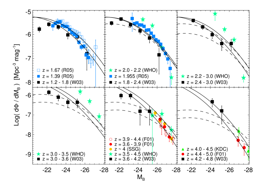
Figure 11.— Running our predicted broad-line luminosity function (determined in § 3, 4) to high redshifts, with either total density (dashed lines) or break luminosity ($L_{\ast}$; solid lines) decreasing exponentially with redshift above $z=2$. In each panel, our prediction is shown for the minimum and maximum redshift of the corresponding interval from the COMBO-17 luminosity function of Wolf et al. (2003) (W03; black squares). Other references for the observations shown are: R05 - Richards et al. (2005), WHO - Warren et al. (1994), F01 - Fan et al. (2001), SSG - Schmidt, Schneider, & Gunn (1995), KDC - Kennefick, Djorgovski, & De Carvalho (1995).

Finally, our fitted form for the evolution of the break luminosity, with $L_{\ast}\propto\exp{(k_{L}\tau)}$, cannot continue to arbitrarily high redshift. At redshifts $z\gtrsim 2-3$, this asymptotes because $\tau\rightarrow 1$, whereas the observed quasar population declines above $z\sim 2$. This difference is not important for most of our calculated observables, as they are either independent of high-redshift evolution or evolve with cosmic time in some fashion as $\propto\int{\dot{n}(L_{\rm peak})\,{\rm d}t}$, with little time and thus negligible contributions to integrated totals at high redshifts. However, some quantities, in particular the high-mass end of the black hole mass function (see § 6), which is dominated by the small number of the brightest quasars at high redshifts, can receive large relative contributions from these terms. Therefore, it is important in estimating these quantities to be aware of the turnover in the quasar density at high redshifts.

We quantify this in Figure 11, where we show the predicted broad-line luminosity function (where the broad-line phase is determined below in § 6) in six luminosity intervals from $z\sim 1.2-4.8$. The intervals are those of the COMBO-17 luminosity function from Wolf et al. (2003), but we further compare to the observed luminosity functions of Warren et al. (1994), Schmidt, Schneider, & Gunn (1995), Kennefick, Djorgovski, & De Carvalho (1995), Fan et al. (2001), and Richards et al. (2005) at the appropriate (labeled) redshifts. At each redshift $z>2$, we take the fitted $\dot{n}(L_{\rm peak})$ distribution above (Equations 21, 22) and rescale it according to an exponential cutoff: either pure density evolution (PDE), $\dot{n}(L_{\rm peak})\rightarrow\dot{n}(L_{\rm peak})\times 10^{-\alpha_{\rm PDE}\,(z-2)}$, or pure peak luminosity evolution (PPLE), $L_{\ast}\rightarrow L_{\ast}\times 10^{-\alpha_{\rm PPLE}\,(z-2)}$. Fitting to the data gives $\alpha_{\rm PDE}\sim 0.65$ and $\alpha_{\rm PPLE}\sim 0.55$, ($\chi^{2}/\nu\approx 1.3$ for both) in reasonable agreement with the density evolution of e.g. Fan et al. (2001). We note that this evolution, extrapolated as far as $z\sim 6$, is consistent also with the constraints on $z\sim 6$ quasars from Fan et al. (2003), especially in the PPLE case.

In each panel, we plot the resulting broad-line luminosity function (see § 4), for both the minimum and maximum redshift of the redshift bin, and both the PPLE (solid lines) and PDE (dashed lines) cases. The degeneracy between these possibilities is well-known, as current observations do not resolve the break in the luminosity function. Furthermore, the predicted luminosity function should be considered uncertain especially at low luminosities, as the quasar lifetime at these luminosities and redshifts can become comparable to the age of the Universe, at which point our formalism for the luminosity function as a function of $\dot{n}(L_{\rm peak})$ becomes inaccurate. However, we are able to make testable predictions, based on differences between the two models in integrated galaxy properties (for example, color-magnitude diagrams of red sequence galaxies at low masses or the fraction of recently formed spheroids as a function of mass and redshift), which distinguish the PPLE and PDE models for the evolution of the quasar luminosity function at $z\gtrsim 2-3$ (Hopkins et al., 2005e). Owing to these degeneracies and the poor constraints on the observed high-redshift luminosity functions, we have not considered them (those at $z>3$) in our fits to $\dot{n}(L_{\rm peak})$, but use them here to roughly constrain the turnover in the quasar density above $z\sim 2$ (i.e. fitting to $\alpha_{\rm PDE}$ and $\alpha_{\rm PPLE}$). Which form of the turnover we use makes little difference in our subsequent analysis, but, as discussed above, including some turnover is important in calculating select quantities such as the extreme high-mass end of the black hole mass function.

3.3. The Observed $N_{\rm H}$ Distribution

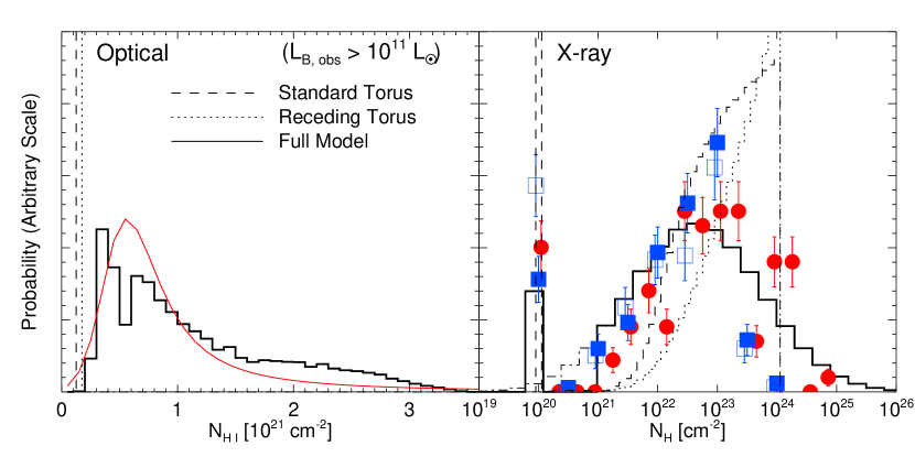
Figure 12.— Left panel: Distribution of column densities expected from the characteristic quasars $L_{\rm peak}\sim L_{\ast}$ of the luminosity function observed in optical samples, for a standard torus model of quasar obscuration (dashed), a receding torus model (dotted), and the distributions of column densities as a function of instantaneous and peak luminosity in our simulations (solid). The distribution of neutral $N_{\rm H\,I}$ values is obtained requiring an observed B-band luminosity $>10^{11}\,L_{\sun}$. The smooth red curve is the best-fit to the $E_{B-V}$ distribution of bright SDSS quasars with $z<2.2$, from Hopkins et al. (2004), rescaled to column densities and plotted about a peak (mode) $N_{\rm H\,I}$ (undetermined in Hopkins et al. 2004) of $N_{\rm H\,I}\approx 0.5\times 10^{21}\,{\rm cm^{-2}}$. The $i$-band absolute magnitude limit imposed in the observed sample, $M_{i}<-22$, corresponds approximately to our plotted B-band limit $L_{B,{\rm obs}}>10^{11}\,L_{\sun}$. Reproduced from Hopkins et al. (2005b). Right panel: Integrated distribution of total (neutral and ionized) column densities expected for a complete hard X-ray sample, from the column densities of our simulations and the $\dot{n}(L_{\rm peak})$ distribution. The distribution below $10^{21}\ {\rm cm^{-2}}$ is shown (dot-dashed line) and re-plotted as a single bin at $N_{\rm H}=10^{20}\ {\rm cm^{-2}}$ for our modeled columns. Data shown are the results of Treister et al. (2004) (blue squares) and Mainieri et al. (2005) (red circles), with assumed Poisson errors. Solid squares assume an intrinsic photon index $\Gamma=1.9$, for the soft X-ray quasar spectrum, open squares $\Gamma=1.7$.

Given the column density distributions and quasar lifetimes calculated from our simulations in § 2, and the quantity $\dot{n}(L_{\rm peak})$ determined above (§ 3.2), we can predict the distribution of column densities observed in a given sample. This will depend not only on the range of observed luminosities and the redshift of the sample, but also on the minimum observed magnitude and frequency (i.e. the selection function) of the sample. For a nearly complete sample or estimate of the luminosity function, for example the hard X-ray luminosity function, at least to $N_{\rm H}\sim 10^{25}\ {\rm cm^{-2}}$, we can integrate the $N_{\rm H}(L,L_{\rm peak})$ distribution over the $\dot{n}(L_{\rm peak})$ distribution (weighted by the lifetime at $L$).

Figure 12 plots the resulting distribution of column densities for this analysis. The left panel reproduces and expands upon a portion of Fig. 3 of Hopkins et al. (2005b), showing the distribution of column densities (scaled linearly) expected from the characteristic quasars $L_{\rm peak}\sim L_{\ast}$ of the luminosity function observed in optical samples, based on the simulated column density distributions as a function of luminosity and peak luminosity (solid black line). Specifically, we plot the distribution of neutral $N_{\rm H\,I}$ values requiring that the observed B-band luminosity be above some reference value $L_{B,{\rm min}}$. The smooth curve shown is the best-fit to the $E_{B-V}$ distribution of bright SDSS quasars with $z<2.2$, from Hopkins et al. (2004). The curve has been rescaled in terms of the column density (inverting our gas-to-dust prescription) and plotted about a peak (mode) $N_{\rm H\,I}$ (undetermined in Hopkins et al. 2004) of $N_{\rm H\,I}\approx 0.5\times 10^{21}\,{\rm cm^{-2}}$. The observationally implied $E_{B-V}$ distribution is determined from fitting to the distribution of photometric reddening in all SDSS bands (i.e. using the five-band photometry as a proxy for spectral fitting) in Sloan quasars, relative to the modal quasar colors at each redshift, for quasars with an absolute magnitude limit $M_{i}<-22$. The $i$-band absolute magnitude limit imposed in the observed sample, $M_{i}<-22$, corresponds approximately to our plotted B-band limit $L_{B,{\rm obs}}>10^{11}\,L_{\sun}$. This estimate does not account for bright but strongly reddened quasars having their colors altered to the point where color selection criteria of quasar surveys will not include them. However, this effect would only serve to bring our distribution into better agreement with observations, as it would slightly lower the high-$N_{\rm H\,I}$ tail. We also consider the predictions of a standard torus model and receding (luminosity-dependent) torus model in the figure (dashed and dotted lines, respectively). These should not be taken literally in this case – they reflect that these phenomenological models do not predict the distribution of low/moderate column densities, but rather assume that all lines of sight not intersecting the torus are “unobscured,” and encounter some constant, small column density (usually chosen to be $N_{\rm H}\sim 10^{20}\,{\rm cm^{-2}}$).

The right panel of 12 shows the integrated distribution (in $\log N_{\rm H}$) for a complete hard X-ray sample, both as predicted from our simulations based on the joint distribution of column density, luminosity, and peak luminosity (solid), and for both the standard torus model (dashed) and receding torus model (dotted) described in § 2.5. The data shown are the results of Treister et al. (2004) (blue squares) and Mainieri et al. (2005) (red circles), with assumed Poisson errors, from multiband Chandra and HST observations of GOODS fields. The solid squares are obtained by assuming an intrinsic photon index for the soft X-ray quasar spectrum of $\Gamma=1.9$, the open squares assuming $\Gamma=1.7$. For the sake of direct comparison with observed distributions, objects with $N_{\rm H}<10^{21}\ {\rm cm^{-2}}$, for which only an upper limit to the column density would be determined in X-ray observations, are grouped together and plotted as a single bin at $N_{\rm H}=10^{20}\ {\rm cm^{-2}}$. The actual distribution below $10^{21}\ {\rm cm^{-2}}$ is shown as a dot-dashed line. We note that our model of the quasar spectrum assumes a photon index $\Gamma=1.9$ in the soft X-ray, but this has no effect on the column densities calculated from the surrounding gas in our simulations.

The agreement between the observed column density distribution and the result of our simulations once the same selection effect is applied supports our model for quasar evolution, and the good agreement extends to both optical and X-ray samples. Probing to fainter luminosities or frequencies less affected by attenuation broadens the column density distribution, as is seen from the inferred column density distributions in the X-ray. This broadening occurs because, at lower luminosities, observers will see both intrinsically bright periods extinguished by larger column densities (broadening the distribution to larger $N_{\rm H}$ values) and intrinsically faint periods with small column densities (broadening the distribution to smaller $N_{\rm H}$ values). The distribution as a function of reference luminosity is a natural consequence of the dynamics of the quasar activity. Throughout much of the duration of bright quasar activity, column densities rise to high levels as a result of the same process that feeds accretion, producing the well-known reddened population of quasars (e.g. Webster et al., 1995; Brotherton et al., 2001; Francis et al., 2001; Richards et al., 2001; Gregg et al., 2002; White et al., 2003; Richards et al., 2003), extending to bright quasars strongly reddened by large $N_{\rm H\,I}$. Furthermore, a significant number of quasars are extinguished from optical samples or attenuated to lower luminosities, giving rise to the distinction between luminosity functions in the hard X-ray, soft X-ray, and optical.

The standard torus model described in § 2.5, although unable to predict the distribution of column densities seen in optically, relatively unobscured quasars, does a fair job of reproducing the observed distribution of X-ray column densities. The parameters of the model are, of course, chosen to reproduce the data shown (the model parameters are taken from Treister et al., 2004). Nevertheless, our prediction is still a better fit to the observed distribution, with $\chi^{2}/\nu\approx 2$ as opposed to $\chi^{2}/\nu\approx 7$ (although the absolute values depend on the estimated systematic errors in the column density estimations). The receding torus model fares even more poorly in reproducing the observed column density distributions, and is ruled out at high significance ($\chi^{2}/\nu\approx 10$), although this can be alleviated if the observed samples are assumed to be incomplete above $N_{\rm H}\sim 10^{23}\,{\rm cm^{-2}}$. This disagreement results because, in order to match the observed scaling of broad-line fraction with luminosity (see § 4 below), this model assumes a larger covering fraction for the torus at lower luminosities, normalized to a similar obscured fraction as the standard torus model near the break in the observed quasar luminosity function. However, since quasars with luminosities below the break dominate the total number counts, this predicts that the cumulative column density distribution must be significantly more dominated by objects with large covering angles, giving a larger Compton-thick population, inconsistent with the actual observed column density distribution.

Although we do not see a significant fraction of extremely Compton-thick column densities $N_{\rm H}\gtrsim 10^{26}\,{\rm cm^{-2}}$ in the distributions from our simulations, our model does not rule out such values. It is possible that bright quasars in unusually massive galaxies or quasars in higher-redshift, compact galaxies which we have not simulated may, during peak accretion periods, reach such values in their typical column densities. Moreover, as our model assumes $\sim 90\%$ of the mass of the densest gas is clumped into cold-phase molecular clouds, a small fraction of sightlines will pass through such clouds and measure column densities similar to those shown for the “cold phase gas” in, e.g. Figure 2 of Hopkins et al. (2005a), $N_{\rm H}\gtrsim 10^{25-26}{\rm cm^{-2}}$.

Furthermore, we have not determined the “shape” at any instant of the obscuration (e.g. the dependence of obscuration on radial direction), as in practice, for most of the most strongly obscured phases in peak merger activity, the central regions of the merging galaxies are highly chaotic. Generally, the scale of the obscuration in the peak merger phases is $\sim 100\,$pc, quite different than that implied by most traditional molecular torus models, but we note that our resolution limits, $\sim 20\,$pc in the dense central regions of the merger, prevent our ruling out collapse of gas in the central regions into a smaller but more dense torus. However, several efforts to model traditional tori through radiative transfer simulations (e.g., Granato & Danese, 1994; Schartmann et al., 2005) suggest significant column densities produced on scales of $\sim 100-200\,$pc, comparable to our predictions, and we note that only the solid angle covered by a torus, not the absolute torus scale, is constrained in the typical phenomenological torus model (e.g. Antonucci, 1993).

Whether the obscuration of bright quasars originates on larger scales than is generally assumed is observationally testable, either through direct probes of polarized scattered light tracing the obscuring/reflecting structure (e.g., Zakamska et al., 2005), or through correlations between obscuration and e.g. host galaxy morphologies and inclinations (e.g., Donley et al., 2005). These larger scales typical of the central regions of a galaxy are widely accepted as the scales of obscuration in starbursting systems (e.g. Soifer et al. 1984a,b; Sanders et al. 1986, 1988a,b; for a review, see e.g. Soifer et al. 1987), which in our modeling is associated with rapid obscured quasar growth and precedes the quasar phase. Thus, it is natural to associate obscuration with these large scales in any picture which associates starbursts and rapid black hole growth or quasar activity, as opposed to the smaller scales $\sim$ pc implied by torus models primarily developed to reproduce observations of quiescent, low-luminosity Type II AGN, which are usually not directly associated with merger activity. These low-luminosity AGN are in a relaxed state, suggesting the possibility that the remaining cold gas in the central regions of our merger remnants will collapse once the violent effects of the merger and bright quasar phase have passed, producing a more traditional small torus in a quiescent nucleus. The central point is that regardless of the form of obscuration, the typical magnitude of the obscuration is a strongly evolving function of time, luminosity, and host system properties, and the observed column density distributions reflect this evolution.

4. Broad-Line Quasars

4.1. Determining the Broad-Line Phase

Optical samples typically identify quasars through their colors, relying on the characteristic non-stellar power-law continua of such objects. However, observations of X-ray selected AGN show a large population of so-called Type 2 AGN, most of which have Seyfert-like luminosities and typical spectra in X-rays and wavelengths longward of $1\,\mu$m (e.g., Elvis et al., 1994), but are optically obscured to the point where no broad lines are visible. Their optical continua, in other words, resemble those of typical galaxies and thus they are not identified by conventional color selection techniques in optical quasar surveys. Traditional unification models (Antonucci, 1993) have postulated a static torus as the explanation for the existence of the Type 2 population, with such objects viewed through the dusty torus and thus optically obscured. Moreover, both synthesis models of the X-ray background (Setti & Woltjer, 1989; Madau et al., 1994; Comastri et al., 1995; Gilli et al., 1999, 2001) and recent direct observations in large surveys (e.g., Zakamska et al., 2004, 2005) indicate the existence of a population of Type 2 quasars, with similar obscuration but intrinsic (unobscured) quasar-like luminosities.

Observations of both radio-loud (Hill, Goodrich, & DePoy, 1996; Simpson, Rawlings, & Lacy, 1999; Willott et al., 2000; Simpson & Rawlings, 2000; Grimes, Rawlings, & Willott, 2004) and radio-quiet (Steffen et al., 2003; Ueda et al., 2003; Hasinger, 2004; Sazonov & Revnivtsev, 2004; Barger et al., 2005; Simpson, 2005) quasars, however, have shown that the broad-line fraction increases with luminosity, with broad-line objects representing a large fraction of all AGN at luminosities above the “break” in the luminosity function and rapidly falling off at luminosities below the break. Modifications to the standard torus unification model explain this via a luminosity-dependent inner torus radius (Lawrence, 1991), but this represents a tunable modification to a purely phenomenological model. Furthermore, as the observations have improved, it has become clear that even these luminosity-dependent torus models cannot produce acceptable fits to the broad line fraction as a function of luminosity (e.g., Simpson, 2005). However, we have shown above that the obscuring column, even at a given luminosity, is an evolutionary effect, dominated by different stages of gas inflow in different merging systems giving rise to varying typical column densities, rather than a single static structure. It is of interest, then, to calculate when quasars will be observed as broad-line objects, and to compare this with observations of broad line quasars and their population as a function of luminosity.

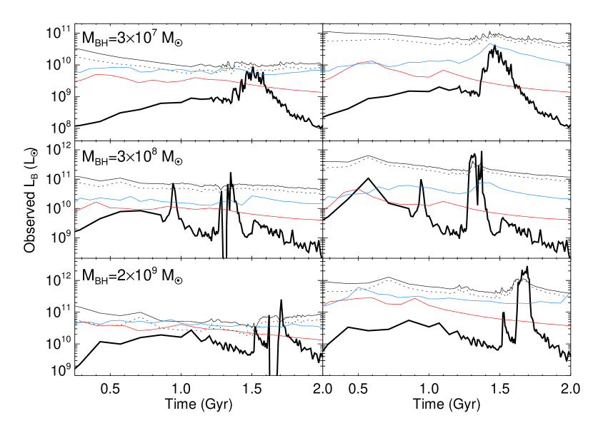
Figure 13.— Intrinsic (right panels) and median attenuated (left panels) B-band luminosity of the quasar (thick line) and host galaxy (integrated over all stars, thin line; ignoring bulge stars, dotted line) as a function of time. Results are shown from three representative simulations: A2, A3, and A5 (see § 2.1) with $q_{\rm EOS}=1.0,\,z_{\rm gal}=0$, and virial velocities $V_{\rm vir}=113,\,160,\ {\rm and}\ 320\,{\rm km\,s^{-1}}$. Each quasar should be observable as a broad-line AGN when $L_{\rm B,\,QSO}\gtrsim L_{\rm B,\,host}$. Colors show the stellar light curve with different gas fractions $f_{\rm gas}=1.0$ (black), $f_{\rm gas}=0.4$ (blue), and $f_{\rm gas}=0.2$ (red); quasar light curves are similar for each gas fraction.

Figure 13 shows the B-band luminosity as a function of time for both the quasars and host galaxies in three representative simulations: the A2, A3, and A5 cases described in detail in § 2.1. These simulations each have $f_{\rm gas}=1.0,\,q_{\rm EOS}=1.0,\,z_{\rm gal}=0$, with virial velocities $V_{\rm vir}=113,\,160\,{\rm and}\ 320\,{\rm km\,s^{-1}}$, with resulting final black hole masses $M^{f}_{\rm BH}=3\times 10^{7},\ 3\times 10^{8},\ {\rm and}\ 2\times 10^{9}\,M_{\sun}$, respectively. The thick line in each case shows the quasar B-band luminosity, and the thin line shows the integrated B-band luminosity of all stars in the galaxy. New stars are formed self-consistently in the simulations according to the ISM gas properties, equation of state and star formation model described in Springel & Hernquist (2003), with the age and metallicity taken from the local star-forming ISM gas, which is enriched by supernova feedback from previous star formation. We then use the stellar population synthesis model of Bruzual & Charlot (2003) to determine the B-band luminosity (the B-band mass-to-light ratio) of new stars based on the stellar age and metallicity. The dotted line shows the result neglecting bulge particles, which must be initialized at the beginning of the simulation with random or uniform ages and metallicities instead of those quantities being determined self-consistently from the simulation physics. The right panels plot the intrinsic values of these quantities, and the left panels plot the median observed values of these quantities, where we have used our method for determining column densities and dust attenuation (§ 2.2) to every star and bulge particle for each line of sight.

Unfortunately, the host galaxy luminosity does not scale with instantaneous and peak quasar luminosity as do, for example, the quasar lifetime and obscuration. Rather, there are important systematic dependencies, the largest of which is the dependence on host galaxy gas fraction. If the host galaxies are more massive, more concentrated, or have a weaker ISM equation of state pressurization, then they will more effectively drive gas into the central regions and maintain high gas densities for longer periods of time, as the deeper potential well or lack of gas pressure requires more heat input from the quasar before the gas can be expelled. These conditions will generally produce a quasar with a larger peak luminosity (final black hole mass), but also form more new stars, meaning that the B-band relation between host and quasar luminosity is roughly preserved.

However, the the black hole consumes only a small fraction of the available gas (comparison of e.g. the stellar mass and black hole mass suggests the black hole consumes $\sim 0.1\%$ of the gas mass), and so, at least above some threshold $f_{\rm gas}\lesssim 0.1$, the quasar peak luminosity does not significantly depend on the galaxy gas fraction (see, e.g. Figure 2 of Robertson et al. 2005b). But, the mass of new stars formed during the merger does strongly depend on the available gas. For example, simulations which are otherwise identical but have initial $f_{\rm gas}=0.2,\ 0.4,\ 0.8,\ 1.0$ (i.e. an increasing fraction of the initial disk mass in gas instead of stars) produce similar peak quasar luminosity and final total stellar mass (within $\sim 30\%$ of one another), reflecting the conversion of most gas into stars and the fact that the peak quasar luminosity is determined more by the depth of the potential well than the total available gas supply. But, the mass of new stars formed in a merger scales roughly as $M_{\ast,\,\rm new}\propto f_{\rm gas}$ (as it must if the initial gas fraction does not change the final total stellar mass), and since young stellar populations dominate the observed B-band luminosity (especially during the peak merger and starburst phases associated with the bright quasar phase of interest), this implies roughly that $L_{B}\propto f_{\rm gas}$.

We demonstrate this explicitly in Figure 13, where we show in each panel the host galaxy and stellar B-band light curves for otherwise identical simulations with different gas fractions, $f_{\rm gas}=0.2\ {\rm(red)},\ 0.4\ {\rm(blue)},\ {\rm and}\ 1.0\ {\rm(black)}$. In each of these cases, the quasar light curve is nearly identical (we show only the $f_{\rm gas}=1.0$ quasar lightcurve, for clarity, but the others are within $\sim 30\%$ of the curve shown at most times, with no systematic offset).

In order for a quasar to be classified as a “broad-line” object, the optical spectrum must be visible and identified as such in the observed sample. This is clearly related to the ratio of quasar to host galaxy luminosity, but the threshold for classification is not obvious. In an X-ray or IR-selected sample, optical follow-up should be able to disentangle host galaxy light and identify quasar broad-line spectra with fluxes a factor of several fainter than the host. However, automated optical selection based on color or morphological criteria might well exclude objects unless the quasar luminosity is a factor of several greater than that of the host galaxy. Therefore, there is significant systematic uncertainty in the theoretical definition of a broad-line quasar. To first order, based on the above arguments, we can classify “broad-line quasars” as objects in which the quasar optical luminosity is larger than some multiple $f_{\rm BL}$ of the host galaxy optical luminosity. Because the relevant ratio is different depending on the survey and selection techniques, we consider the range $f_{\rm BL}=0.3-3$, with a rough median $f_{\rm BL}=1$. Furthermore, because our simulations do not allow us to model the broad-line regions of the quasar or spectral line structures as influenced by e.g. reddening and dust absorption, we adopt the B-band luminosity of the quasar and host galaxy as a proxy for optical luminosity and more complex (but often quite sample-specific) color and morphological selection criteria.

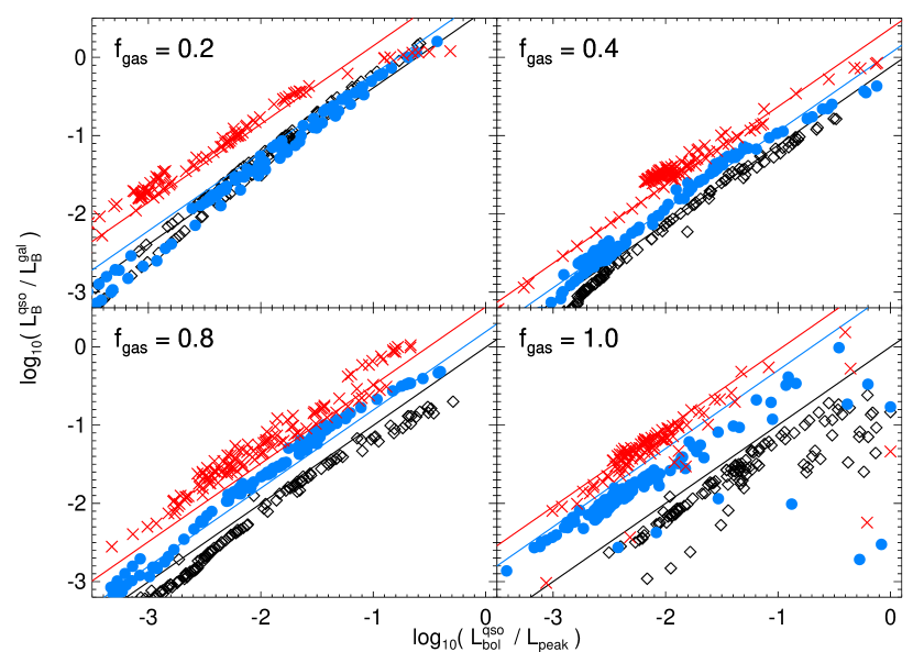
Figure 14.— Ratio of observed (attenuated) B-band quasar luminosity to host galaxy luminosity as a function of the ratio of instantaneous to peak quasar bolometric luminosity. Results are from simulations A2 (black diamonds), A3 (blue circles), and A5 (red $\times$’s) (the same simulations shown in Figure 13) with $q_{\rm EOS}=1.0,\,z_{\rm gal}=0$, and virial velocities $V_{\rm vir}=113,\,160,\ {\rm and}\ 320\,{\rm km\,s^{-1}}$. Each panel shows the same simulations except for a different initial gas fraction $f_{\rm gas}=0.2,\ 0.4,\ 0.8,\ 1.0$ as labeled. Solid lines are the predictions of Equation 26.

In Figure 13, the B-band host galaxy luminosity is quite flat as a function of time, relative to the quasar B-band luminosity, and is roughly given by $L_{B}^{\rm gal}/L_{\sun}\sim M_{\ast,\,\rm new}/M_{\sun}$, where $M_{\ast,\,\rm new}$ is the mass of new stars formed in the merger. As noted above, this scales approximately linearly with initial gas fraction at fixed final total stellar mass $M_{\ast}$, giving $L_{B}^{\rm gal}/L_{\sun}\approx c_{\rm gal}(M_{\ast}/M_{\sun})f_{\rm gas}$, where $c_{\rm gal}$ is a correction of order unity which we can fit from the simulations (essentially a mean mass-to-light ratio for the newly formed stars). The bolometric correction of the quasar is usually defined by $L_{\rm bol}^{\rm qso}=c_{B}L_{B}^{\rm qso}$, and the quasar peak luminosity is $L_{\rm peak}=c_{L}\,L_{\rm Edd}(M_{\rm BH}^{f})$, where again $c_{L}$ is a correction factor of order unity which we can calculate from our form for the quasar lifetime (see Equation 10) or measure in the simulations.

If we require that the quasar B-band luminosity be larger than a factor $f_{\rm BL}$ of the host galaxy B-band luminosity, we obtain

$$L_{\rm bol}^{\rm qso}/L_{\sun}>f_{\rm BL}c_{B}\,c_{\rm gal}(M_{\ast}/M_{\sun})f_{\rm gas}.$$ (23)

Dividing this through by $L_{\rm peak}$, we have

$$\frac{L_{\rm bol}^{\rm qso}}{L_{\rm peak}}\gtrsim 0.4\,f_{\rm gas}\,f_{\rm BL}\ {\Bigl{(}}\frac{c_{\rm gal}}{1.0}{\Bigr{)}}{\Bigl{(}}\frac{c_{B}}{12.0}{\Bigr{)}}{\Bigl{(}}\frac{M_{\rm BH}^{f}/M_{\ast}}{0.001}{\Bigr{)}}^{-1}{\Bigl{(}}\frac{c_{L}}{1.24}{\Bigr{)}}^{-1}.$$ (24)

We can test this scaling relation against the results of our simulations, and do so in Figure 14. Rearranging the equations above gives

$$\frac{L_{B}^{\rm qso}}{L_{B}^{\rm gal}} \approx \ 3.4\,f_{\rm gas}^{-1}\,\frac{L_{\rm bol}^{\rm qso}}{L_{\rm peak}}$$ (25)

$$\times{\Bigl{(}}\frac{c_{\rm gal}}{1.0}{\Bigr{)}}^{-1}{\Bigl{(}}\frac{c_{B}}{12.0}{\Bigr{)}}^{-1}{\Bigl{(}}\frac{M_{\rm BH}^{f}/M_{\ast}}{0.001}{\Bigr{)}}{\Bigl{(}}\frac{c_{L}}{1.24}{\Bigr{)}},$$

which we can compare to our direct calculation of $L_{B}^{\rm qso}/{L_{B}^{\rm gal}}$ and $L_{\rm bol}^{\rm qso}/L_{\rm peak}$ for each simulation snapshot.

Ultimately, we are not interested so much in the intrinsic B-band luminosity of the quasar and host galaxy, but rather the observed luminosities; i.e. we are interested in the ratio ${L_{B,\rm\ obs}^{\rm qso}}/{L_{B,\rm\ obs}^{\rm gal}}=({L_{B}^{\rm qso}}/{L_{B}^{\rm gal}})\,(\exp\{-(\tau_{Q}-\tau_{G})\})$, where $\tau_{Q}$ and $\tau_{G}$ are “effective” optical depths which we use to denote the mean attenuation of quasar and host galaxy B-band luminosities, respectively. We have considered the distribution of column densities attenuating the quasar as a function of instantaneous and peak quasar luminosity in detail in § 2.3 above; the attenuation of the host galaxy as a function of luminosity, observed band, halo mass, and star formation rate are discussed in detail in Jonsson et al. (2005). Combining these fits gives, roughly, $(\exp\{-(\tau_{Q}-\tau_{G})\})\sim(M_{\rm BH}^{f}/10^{8}\,M_{\sun})^{0.16}$, but a better approximation can be determined directly from the simulations.

This scaling can be understood roughly using toy models of uniformly mixed luminous sources within the galaxy described by Jonsson et al. (2005), after accounting for the fact that the luminosity (star formation rate) dependent portion of the attenuation scales with luminosity in a similar manner to our quasar attenuation (compare our $\tau_{Q}\propto N_{\rm H}\propto L_{\rm qso}^{0.43-0.54}$ to their $\tau_{G}\propto L_{\rm B,\ gal}^{0.55}$). The key consequence of this is that more massive systems (higher bulge and black hole masses) have their host galaxy light proportionally more attenuated in mergers, meaning that (as suggested by the comparison of light curves in Figure 13) the quasar is more likely to be observed with an optical luminosity larger than that of its host.

Figure 14 plots the ratio of the observed (attenuated) B-band quasar luminosity to the observed host galaxy B-band luminosity as a function of the ratio of instantaneous to peak quasar bolometric luminosity. We show the results for four different gas fractions $f_{\rm gas}=0.2,\ 0.4,\ 0.8,\ 1.0$ as labeled. For each gas fraction, we consider our simulations A2 (black diamonds), A3 (blue circles), and A5 (red $\times$’s) (the same simulations shown in Figure 13) with $q_{\rm EOS}=1.0,\,z_{\rm gal}=0$, and virial velocities $V_{\rm vir}=113,\,160\,{\rm and}\ 320\,{\rm km\,s^{-1}}$, using the labeled initial gas fraction. The colored lines in each panel show the predictions of combining the scalings expected for the intrinsic luminosities (Equation 25) and attenuations as above, giving

$$\frac{L_{\rm B,\ obs}^{\rm qso}}{L_{\rm B,\ obs}^{\rm gal}}=7.9\,\frac{1}{f_{\rm gas}}\,{\Bigl{(}}\frac{M_{\rm BH}^{f}}{10^{8}\,M_{\sun}}{\Bigr{)}}^{0.2}\ \frac{L}{L_{\rm peak}},$$ (26)

where the colored lines each use the $M_{\rm BH}^{f}$ and $f_{\rm gas}$ of the simulation of the corresponding color and panel. This scaling provides a good estimate of the observed optical quasar-to-galaxy luminosity ratio, including the complicated effects of attenuation, evolving mass-to-light ratios, metallicities, and host galaxy properties, as a function of gas fraction, final black hole mass, and the ratio of the current to peak quasar luminosity. Although, for clarity, we have not shown a range of simulations varying other parameters, we find that this scaling is robust to the large number of quantities we have considered in our simulations – there are systematic offsets in e.g. $L_{\rm peak}$ and $M_{\rm BH}^{f}$ with changes such as e.g. different ISM equations of state, but the scaling in terms of $L_{\rm peak}$ and $M_{\rm BH}^{f}$ is unchanged.

Because the ratio of observed quasar and host galaxy B-band luminosities in our simulations obeys the scaling of Equation 26, we can use it to predict the properties of “broad-line” quasars, defined by $L_{\rm B,\ obs}^{\rm qso}>f_{\rm BL}L_{\rm B,\ obs}^{\rm gal}$. To do so, however, we must assume a typical host galaxy gas fraction. Unfortunately, because our empirical modeling in terms of the quasar lifetime as a function of $L$ and $L_{\rm peak}$ does not have a systematic dependence on host galaxy gas fraction (see § 2.4), we have no constraint on this parameter. It is, however, convenient for several reasons to consider $f_{\rm gas}=0.3$ as a typical value for bright quasars.

First, such a gas fraction is capable of yielding the brightest observed quasars; second, scaling a Milky-Way like disk with the observed $z=0$ gas fraction $\sim 0.1$ to the redshifts of peak quasar activity gives a similar gas fraction (e.g., Springel et al., 2005a); third, gas fractions $\gtrsim 30\%$ in major mergers are needed to explain the observed fundamental plane (Robertson et al. 2005c, in preparation), kinematic properties (Cox et al. 2005c, in preparation), and central phase space densities (Hernquist, Spergel & Heyl 1993) of elliptical galaxies; fourth, this choice implies that the brightest quasars with $M_{\rm BH}^{f}\sim 10^{10}\,M_{\sun}$ attain observed B-band luminosities $\sim 1000$ times that of their hosts at their peaks, as is observed (e.g., McLure & Dunlop, 2004). Finally, and most important, the assumed $f_{\rm gas}$ and $f_{\rm BL}$ are degenerate in our predictions for the broad-line population, as they both enter linearly in the ratio of host galaxy to quasar B-band luminosity. Therefore, the range of $f_{\rm BL}=0.3-3$ which we consider (for a fixed median $f_{\rm gas}=0.3$) can be equivalently considered, for a fixed median $f_{\rm BL}=1$, to represent a theoretical uncertainty in the host galaxy gas fraction, $f_{\rm gas}=0.1-0.9$; i.e. spanning the range from present, relatively gas-poor Milky-Way like disks to almost completely gaseous disks. This, then, gives for our “broad-line” criterion,

$$\frac{L}{L_{\rm peak}}\gtrsim 0.2\,{\Bigl{(}}\frac{f_{\rm BL}}{1.0}{\Bigr{)}}\,{\Bigl{(}}\frac{f_{\rm gas}}{0.3}{\Bigr{)}}\,{\Bigl{(}}\frac{M_{\rm BH}^{f}}{10^{7}\,M_{\sun}}{\Bigr{)}}^{-0.2}.$$ (27)

The “broad-line” phase is thus, as is clear from Figure 13 and implicit in our definition of the broad-line phase, closely associated with the final “blowout” stages of quasar evolution, when the mass of the quasar reaches that corresponding to its location on the $M_{\rm BH}-\sigma$ relation and gas is expelled from the central regions of the galaxy, shutting down accretion (Di Matteo et al., 2005). We note that combining the equation above with our fitted quasar lifetimes gives an integrated time when the quasar would be observable as a broad line object of $t_{\rm BL}\sim 10-20$ Myr, in good agreement with the optically observable bright quasar lifetimes we calculate directly from our quasar light curves, including the effects of attenuation, and with empirical estimates of the quasar lifetime which are based directly on optically-selected, broad-line quasar samples.

The $({M_{\rm BH}^{f}}/{10^{7}\,M_{\sun}})^{0.2}$ term in the above equation reflects the fact that, below a certain peak luminosity, quasars are less likely to reach luminosities above that of the host galaxy, as can be seen in the uppermost panels of Figure 13 for a final black hole mass of $M^{f}_{\rm BH}=3\times 10^{7}$ – i.e. the smallest AGN are proportionally less optically luminous than their hosts. This does not imply that such systems are not inherently broad-line objects, but only that the host galaxy light will increasingly dominate at lower luminosities. We also caution against extrapolating this to large or small $M_{\rm BH}^{f}$, as the attenuation becomes more difficult to predict at these peak luminosities, and the linear formula above is not always accurate (see Figure 14).

We can use this estimate of the broad-line phase and our model of the quasar lifetime to calculate the total energy radiated in this bright, optically observable stage following the calculation of § 2.4, but with a minimum luminosity determined by Equation 27. This gives an integrated fraction $\sim 0.3-0.4$ ($\sim\exp\{-0.2\,f_{\rm BL}\,(f_{\rm gas}/0.3)/\alpha_{L}\}$) of the total radiant energy emitted during the broad-line phase. Thus, despite the short duration of this optical quasar stage, a large fraction of the total radiated energy is emitted (as it represents the final $e$-folding in the growth of the black hole) when most of the final black hole mass (§ 2.4) is accumulated. Accounting for the luminosity dependence of our bolometric corrections (with the optical fraction of the quasar energy increasing with bolometric luminosity) as well as the small fraction of objects observable at lower luminosities (with larger typical obscuring column densities) increases this fraction to as much as $\sim 0.6-0.7$ for bright quasars. Therefore, despite the fact that the duration of the optically observable broad-line quasar phase may be $\sim 1/10$ that of the obscured quasar growth phase, the changing quasar luminosity over this period and non-trivial quasar lifetime as a function of luminosity implies only small corrections to counting arguments such as that of Soltan (1982), which rely on the total observed optical quasar flux density to estimate the relic supermassive black hole density.

4.2. The Broad-Line Fraction as a Function of Luminosity

By estimating the time that a quasar with some $L_{\rm peak}$ will be observable as a broad-line quasar at a given luminosity, we can then calculate the broad-line quasar luminosity function in the same fashion as the complete quasar luminosity function in § 3.2. Instead of the full quasar lifetime ${\rm d}t/{\rm d}\log{L}$, we consider only the time during which broad-lines would be observed (i.e. that the quasar spectrum would be recognized as opposed to the host galaxy spectrum), as identified in our simulations (§ 4.1).

For a sample selected in hard X-rays (i.e. the selection function only being relevant at column densities $\gtrsim 10^{24}\ {\rm cm^{-2}}$), we show the resulting “broad-line” luminosity function in Figure 9 (cyan dot-dashed lines), and compare it to the broad-line quasar luminosity function identified in the hard X-ray luminosity function of Barger et al. (2005). The agreement is good at all luminosities, and our model explains both the fact that broad-line quasars dominate the luminosity function at luminosities well above the “break” in the luminosity function, and the downturn in the broad-line quasar population at luminosities below the peak. Essentially, the broad-line quasar population more closely traces the shape of the $\dot{n}(L_{\rm peak})$ distribution, giving rise to the observed behavior as a dual consequence of luminosity-dependent quasar lifetimes and the evolutionary nature of quasar obscuration in our simulations.

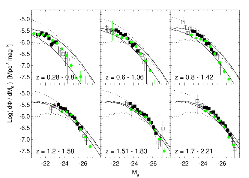
Figure 15.— Broad-line quasar luminosity function of Richards et al. (2005) from the 2dF-SDSS (2SLAQ) survey (black squares) and that of Croom et al. (2004) (green circles) from the 2dF survey, compared to our predicted “broad-line” luminosity function from our determination of the relative quasar and host galaxy luminosities in our simulations (solid line), where we estimate that quasars are observable as “broad-line” objects when their observed B-band luminosity is greater than a factor $f_{\rm BL}$ of that of the host galaxy, Solid lines are shown for the minimum and maximum observed redshift in each bin (as labeled), assuming $f_{\rm BL}=1$. Dotted lines show the result for $f_{\rm BL}=0.3$ and $f_{\rm BL}=3$, at the mean redshift of the bin, i.e. corresponding to “broad-line” luminosity functions in surveys which are complete to quasars with observed optical luminosity $\sim 0.3$ and $3$ times that of the host galaxy, respectively, or alternatively reflecting nearly complete theoretical uncertainty regarding merging galaxy gas fractions ($f_{\rm gas}=0.1-0.9$). Open squares are observations with uncertain incompleteness corrections in Richards et al. (2005).

Figure 15 compares our theoretical predictions to the 2dF-SDSS (2SLAQ) g-band luminosity function of broad-line quasars from Richards et al. (2005) (black squares), as well as the B-band luminosity function from Croom et al. (2004) (green circles), at several redshifts from $z\sim 0.3-2$, over which range the surveys are expected to be relatively complete (for broad-line quasars). The 2dF-SDSS result is the most recent determination of the broad-line luminosity function, but compares well with previous determinations by, e.g., Boyle et al. (1988), Koo & Kron (1988), Marano, Zamorani, & Zitelli (1988), Boyle et al. (1990), Boyle, Jones, & Shanks (1991), Zitelli et al. (1992), Boyle et al. (2000), and Croom et al. (2004). Open squares correspond to bins in luminosity which have been corrected for incompleteness following Page & Carrera (2000), but this correction is uncertain as the bins are not uniformly sampled. We compare this at each redshift to the prediction of our determination of the quasar “broad-line” phase, where we estimate that the quasar is observable as a broad line object when its observed B-band luminosity is greater than a factor $f_{\rm BL}=1$ of that of the host galaxy. We calculate this for both the minimum and maximum observed redshift of each bin to show the range owing to evolution of the luminosity function over each interval in redshift. The systematic uncertainty in our prediction can be estimated from the dotted lines, which show the prediction (at the mean redshift of the bin) if we instead require the observed quasar B-band luminosity to be above a factor of 0.3 (upper lines) or 3 (lower lines) of the observed host galaxy B-band luminosity, which as discussed in § 4.1 can alternatively be considered an uncertainty in host galaxy gas fraction, with $f_{\rm gas}=0.1$ and $f_{\rm gas}=0.9$, respectively.

The agreement at all luminosities and redshifts shown is encouraging, given the simplicity of our determination of the broad-line phase from the simulations, but the systematic uncertainties are large, emphasizing the importance of calculating detailed selection effects in contrasting e.g. “broad-line” samples from optical and X-ray surveys, as opposed to assuming a constant obscured fraction at a given luminosity based on the ratio of luminosity functions as has been adopted in previous phenomenological models. The difference between different choices of $f_{\rm gas}$ is suppressed at the high luminosity (and correspondingly high redshift) end of the luminosity function, because the quasar-to-galaxy B-band luminosity ratio scales as $\propto(M_{\rm BH}^{f})^{0.2}$; i.e. regardless of the choice of $f_{\rm BL}$, quasars increasingly overwhelm their host galaxy in large systems near their peak luminosity. However, at low luminosity, the predictions rapidly diverge, implying that a measurement of the faint end of the broad-line quasar luminosity function, with a reliable calibration of $f_{\rm BL}$, can constrain the typical gas fractions of quasar host galaxies and the evolution of these gas fractions with redshift.

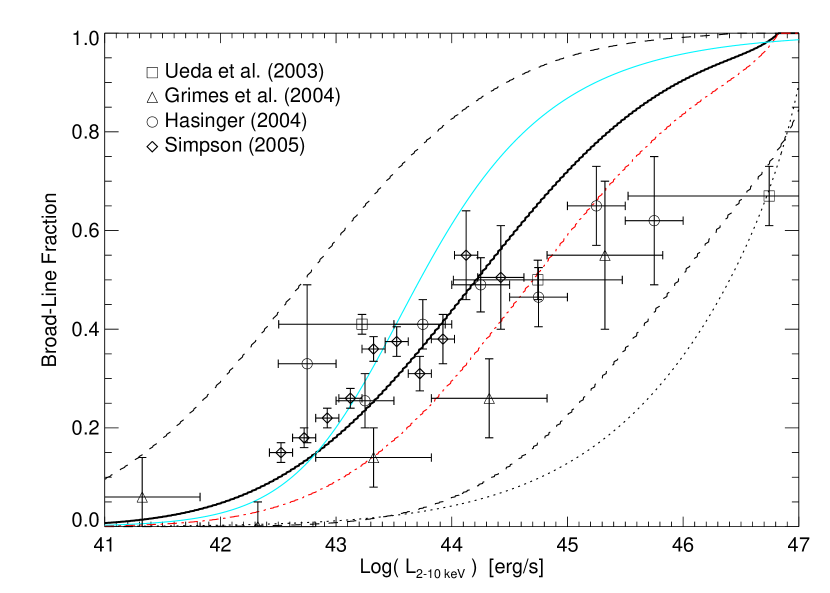
Figure 16.— Predicted “broad-line” fraction of a complete X-ray sample at low $z\lesssim 0.3$ redshift, from our simulations (where the object is observable as a broad-line quasar when it has an observed B-band luminosity greater than a factor $f_{\rm BL}=1.0$ of that of its host galaxy), is shown (thick black line). The results, changing our $f_{\rm BL}$ to 0.3 and 3.0 are shown, or equivalently of assuming a host galaxy gas fraction $f_{\rm gas}=0.1$ or 0.9 instead of $\sim 0.3$ (dashed), as are the results assuming a “light bulb” model where quasars spend a fixed time $t_{Q}=20$ Myr as broad line objects with a luminosity of $L_{\rm peak}$ (dotted). For comparison, the (scaled to 2-10 keV luminosity) observations of Ueda et al. (2003) (squares), Hasinger (2004) (circles), Grimes, Rawlings, & Willott (2004) (triangles), and Simpson (2005) (diamonds) are shown. The predicted result at higher redshift ($z\gtrsim 1$) is shown (red dot-dashed line), offset owing to the shift in break luminosity of the luminosity function with redshift. The best-fit luminosity-dependent torus model, fitted to the data, is shown as the solid cyan line. The best-fit static torus model is a constant broad-line fraction $\sim 0.3$ (not shown for clarity).

By dividing out the predicted luminosity function $\phi_{HX}$, we can estimate the fraction of “broad line” objects observed in reasonably complete X-ray samples as a function of luminosity. This is shown in Figure 16, where for ease of comparison we have shown the broad-line fraction as a function of hard X-ray (2-10 keV) luminosity. Our prediction, based on determining the time a quasar with a given luminosity $L$ and peak luminosity $L_{\rm peak}$ in our simulations will be observable with a B-band luminosity greater than a fraction $f_{\rm BL}=1.0$ of the host galaxy observed B-band luminosity, is shown as the thick black line. This is compared to the observations of Ueda et al. (2003) (squares), Hasinger (2004) (circles), Grimes, Rawlings, & Willott (2004) (triangles), and Simpson (2005) (diamonds). The data from Hasinger (2004) has been scaled from soft X-ray (0.5-2 keV) using our bolometric corrections, and the data from Grimes, Rawlings, & Willott (2004) and Simpson (2005) have been converted from [O iii] luminosity as in Simpson (2005) using the mean correction for Seyfert galaxies (Mulchaey et al., 1994), $L_{\rm[O\,III]}=0.015\times L_{\rm 2-10\,keV}$.

We also plot as upper and lower dashed lines the results of changing $f_{\rm BL}$, the fraction of the host galaxy B-band luminosity above which the quasar B-band luminosity must be observed for identification as a “broad-line” object, considering $f_{\rm BL}=0.3,\ {\rm and}\ 3$, respectively. We determine this for the low-redshift $z\lesssim 0.3$ quasar distribution, from which most of the data are drawn. The red dot-dashed line shows the difference at high redshift, if just $z\gtrsim 1$ quasars are considered (for $f_{\rm BL}=1$). The broad-line fraction is systematically lower, primarily because the break luminosity in the luminosity function moves to higher luminosity with redshift, meaning that at a fixed luminosity below the break, a smaller fraction of observed objects are at $L\sim L_{\rm peak}$ in the “blowout” phase of peak optical quasar luminosity. Finally, the dotted line shows the results assuming a “light bulb” model for the broad-line phase (but still using our $\dot{n}(L_{\rm peak})$ distribution, otherwise this translates to a constant obscured fraction with luminosity) lifetimes, with a fixed broad-line lifetime of $t_{Q}=20\,$Myr.

The prediction of the most basic torus model, with constant broad-line fraction $\sim 0.36$, is ruled out to high significance ($\chi^{2}/\nu=18.5,\ 17.2$ if we consider all data points, or if we consider only the most well-constrained data, from Simpson [2005], respectively). Furthermore, the solid cyan line shows the best-fit luminosity-dependent torus model, in which the broad line fraction is given by (e.g., Simpson, 1998; Grimes, Rawlings, & Willott, 2004)

$$f=1-1/\sqrt{1+3L/L_{0}},$$ (28)

where $L_{0}$ is the luminosity where the number of broad line objects is equal to the number of non-broad line objects. This fit is at best marginally acceptable over a narrow range in luminosities ($\chi^{2}/\nu=14.0,\ 7.3$). Modified luminosity-dependent, receding torus models have been proposed which give a better fit to the data by, for example, allowing the torus height to vary with luminosity (e.g., Simpson, 2005), but there is no physical motivation for these changes, and they introduce such variation through additional free parameters that allow a curve of essentially arbitrary slope to be fitted to the data.

However, the prediction of our model agrees reasonably well ($\chi^{2}/\nu=4.0,\ 1.2$) with the observations over the entire range covered, a span of six orders of magnitude in luminosity. We emphasize that our prediction, which matches the data better than standard torus models that are actually fitted to the data, is not a fit to the observations. Instead, it is derived from the physics of our simulations, including black hole accretion and feedback which are critical in driving the “blowout” phase which constitutes most of the time a quasar is visible as a “broad-line” object by our estimation, and from the $\dot{n}(L_{\rm peak})$ distribution implied by our model of quasar lifetimes and the bolometric quasar luminosity function. The agreement suggests that our choice of the parameter combination $f_{\rm BL}f_{\rm gas}=0.3$ is a good approximation. As noted above, this implies that calibrating $f_{\rm BL}$ for an observed sample, combined with the mean broad-line fraction and our modeling, can provide a constraint (albeit model-dependent) on the host galaxy gas fraction of quasars at a given redshift, which cannot necessarily be directly measured even with difficult, detailed host galaxy probes, as gas is rapidly converted into stars throughout the merger. The uncertainty plotted, while large, actually represents a larger theoretical uncertainty – as discussed above, if an observational sample were well-defined such that it were complete to broad-line objects with observed optical luminosity above a fraction $f_{\rm BL}$ of the host galaxy luminosity, the range we consider would correspond to a range $f_{\rm gas}=0.1-0.9$ in the quasar host galaxy gas fraction, which the observations could then constrain.

In our modeling, the broad line fraction as a function of luminosity does not depend sensitively on the observed luminosity function, as evidenced by the relatively similar prediction at high redshift. The evolution we do predict with redshift, in fact, agrees well with that found by Barger et al. (2005) over the redshift range $z=0.1-1.2$ (see also La Franca et al. 2005), an aspect of the observations which is not reproduced in any static or luminosity-dependent torus model but follows from the evolution of the quasar luminosity function in our picture for quasar growth. However, we do caution that gas fractions may systematically evolve with redshift, and as discussed above, a higher gas fraction will give generally shorter “broad-line” lifetimes using our criteria of quasar optical luminosity being higher than some fraction of the host galaxy luminosity, which will also contribute to the evolution in the mean “broad-line” fraction with redshift. Finally, neglecting the role of luminosity-dependent quasar lifetimes gives unacceptable fits to the data ($\chi^{2}/\nu=66.0,\ 77.5$), as the broad-line fraction as a function of luminosity is a consequence of both the evolution of obscuration and the dependence of lifetime on luminosity.

Our model for quasar evolution provides a direct physical motivation for the change in broad line fraction with luminosity and suggests that it is not a complicated selection effect. As an observational sample considers higher luminosities (i.e. approaches and passes the “break” in the observed luminosity function), a comparison of the luminosity function and the underlying $\dot{n}(L_{\rm peak})$ shows that it is increasingly dominated by sources near their peak luminosity in the final stages of Eddington limited growth. The final stages of this growth expel the large gas densities obscuring the quasar, rendering it a bright, optically observable broad-line object for a short time. Therefore, we expect that the fraction of broad-line objects should increase with luminosity in quasar samples, as indicated by the observations.

Figure 17.— Predicted “obscured” fraction (solid line) in an X-ray sample with identical redshift and luminosity range to that of Ueda et al. (2003), as a function of hard X-ray (2-10 keV) luminosity. Vertical error bars show Poisson errors estimated from the total time at a given luminosity across all our simulations (absolute values of the error bars should not be taken literally). The “obscured” fraction is defined as the fraction of quasars with X-ray column densities $N_{\rm H}>10^{22}\,{\rm cm^{-2}}$ in bins of $\Delta\log{L_{2-10\,{\rm keV}}}$. The observations from Ueda et al. (2003) are shown as black squares.

Many observational measures do not consider a direct optical analysis of the quasar spectrum in estimating the fraction of broad-line objects as a function of luminosity. For example, Ueda et al. (2003) adopt a proxy, classifying as “obscured” any quasars with an X-ray identified column density $N_{\rm H}>10^{22}\,{\rm cm^{-2}}$, and as “unobscured” quasars below this column density. We can compare to their observations, using the column density distributions as a function of luminosity from our simulations, which cover the entire range in luminosity of the observed sample. Specifically, we use a Monte Carlo realization of these distributions, employing our fitted $\dot{n}(L_{\rm peak})$ distribution at each redshift to produce a list of quasar peak luminosities and then generating all other properties based on the probability distribution of a given property in simulations with a similar peak luminosity. We describe this methodology in detail in § 8, and provide several such mock quasar distributions at different redshifts.

In Figure 17, we compare our estimated “obscured” and “unobscured” fractions as a function of hard X-ray luminosity, using the same definitions as well as redshift and luminosity limits as the observed sample. The solid line shows our prediction, with vertical error bars representing Poisson errors, where the number of “counts” is proportional to the total time spent by simulations at the plotted luminosity (the absolute value of these errors should not be taken seriously). The “obscured” fraction is determined in bins of luminosity $\Delta\log L_{2-10\ {\rm keV}}=0.5$. Despite our large number of simulations, there is still some artificial “noise” owing to incomplete coverage of the merger parameter space, namely the apparent oscillations in the obscured fraction. However, the mean trend agrees well with that observed (black squares), suggesting that the success of our modeling in reproducing the fraction of “broad line” objects as a function of luminosity is not a consequence of the definitions chosen above. We do not show the predictions of the standard and luminosity-dependent torus models, as (because essentially any line of sight through the torus encounters a column density $N_{\rm H}>10^{22}\,{\rm cm^{-2}}$) the predictions of these models are identical to those shown and compared to the same observations in Figure 16.

Our prediction that the fraction of broad-line objects should rise with increasing luminosity is counterintuitive, given our fitted column density distributions in which typical (median) column densities increase with increasing luminosity. This primarily owes to the simplicity of our $N_{\rm H}$ fits; we assume the distribution is lognormal at all times, but a detailed inspection of the cumulative (time-integrated) column density distribution shows that at bright (near-peak) luminosities, the distribution is in fact bimodal (see e.g. Figure 3 of Hopkins et al. 2005b and Figure 2 of Hopkins et al. 2005d), representing both the heavily obscured growth phase and the “blowout” phase we have identified here as the “broad line” phase. Over most of a simulation, we find the general trend shown in Figure 3 and discussed above, namely that typical column densities increase with intrinsic (unobscured) luminosity. This is because the total time at moderate to large luminosities is dominated by black holes growing in the obscured/starburst stages; here, the same gas inflows fueling black hole growth also give rise to large column densities and starbursts which obscure the black hole activity. However, when the quasar nears its final, peak luminosity, there is a rapid “blowout” phase as feedback from the growing accretion heats the surrounding gas, driving a strong wind and eventually terminating rapid accretion, leaving a remnant with a black hole satisfying the $M_{\rm BH}-\sigma$ relation. This can be identified with the traditional bright optical quasar phase, as the final stage of black hole growth with a rapidly declining density (allowing the quasar to be observed in optical samples), giving typical luminosities, column densities, and lifetimes of optical quasars. In these stages, larger luminosities imply more violent “blowout” events, i.e. a brighter peak luminosity quasar more effectively expels the nearby gas and dust, rendering a dramatic decrease in column density at these bright stages (see Hopkins et al. 2005f).

We are essentially modeling this bimodality in more detail by directly determining the “broad-line” phase from our simulations. However, the broad line fraction-luminosity relation we predict is also a consequence of the more complicated relationship between column density, peak luminosity, and bolometric and observed luminosity, as opposed to the predictions from a model with correlation between $N_{\rm H}$ and only observed luminosity. The key point is that we find, near the peak luminosity of the quasar, as feedback drives away gas and slows down accretion, the typical column densities fall rapidly with luminosity in a manner similar to that observed. In our model for the luminosity function, quasars below the observed “break” are either accreting efficiently in early stages of growth or are in sub-Eddington phases coming into or out of their peak quasar activity. Around and above the break, the luminosity function becomes dominated by sources at high Eddington ratio at or near their peak luminosities. Based on the above calculation, we then expect what is observed, that in this range of luminosities, the fraction of objects observed with large column densities will rapidly decrease with luminosity as the observed sample is increasingly dominated by sources at their peak luminosities in this blowout phase. This also further emphasizes that the evolution of quasars dominates over static geometrical effects in determining the observed column density distribution at any given luminosity.

Finally, if host galaxy contamination were not a factor, we would expect from our column density model that, at low luminosities ($L\lesssim 10^{10}\,L_{\sun}$, well below the range of most observations shown), the broad-line fraction would again increase (i.e. the obscured fraction would decrease), as the lack of gas to power significant accretion would also imply a lack of gas to produce obscuring columns. However, at these luminosities, typical of faint Seyfert galaxies or LINERs, our modeling becomes uncertain; it is quite possible, as discussed previously, that cold gas remaining in relaxed systems could collapse to form a traditional dense molecular torus on scales $\sim\,$pc, well below our resolution limits. Furthermore, host galaxy light is likely to overwhelm any AGN broad-line contribution, and selection effects will also become significant at these luminosities.

4.3. The Distribution of Active Broad-Line Quasar Masses

Our determination of the “broad-line” or optical phase in quasar evolution allows us to make a further prediction, namely the mass distribution of currently active broad-line quasars. At some redshift, the total number density of observed, currently active broad-line quasars with a given $L_{\rm peak}$ will be (in the absence of selection effects)

$$n_{\rm BL}(L_{\rm peak})\approx\dot{n}(L_{\rm peak})\,t_{\rm BL}(L_{\rm peak}),$$ (29)

where $t_{\rm BL}(L_{\rm peak})$ is the total integrated time that a quasar with peak luminosity $L_{\rm peak}$ spends as a “broad-line” object (using our criterion for the ratio of the observed quasar B-band luminosity to that of the host galaxy), given by integrating our formulae in § 4.1 or directly calculated from the simulations. Since we have determined roughly that a quasar should be observable as a “broad-line” object at times with $L\gtrsim 0.2\,L_{\rm peak}$ primarily just after it reaches its peak luminosity, in the “blowout” phase of its evolution, we expect the instantaneous black hole mass at the time of observation as a broad-line quasar to be, on average, $M^{\rm BL}_{\rm BH}\approx M^{f}_{\rm BH}(L_{\rm peak})$, where $M^{f}_{\rm BH}\sim M_{\rm Edd}(L_{\rm peak})$ modulo the order unity corrections described in § 2.4. Using our fitted $\dot{n}(L_{\rm peak})$ distribution from the luminosity function, extrapolated to low redshift ($z\sim 0$), and combining it with the integrated “broad-line” lifetimes from our simulations as above, we obtain the differential number density of sources in a logarithmic interval in $L_{\rm peak}$. Finally, we use our Equation 10 for $M^{f}_{\rm BH}(L_{\rm peak})$ determined from our fitted quasar lifetimes (demanding that $E_{\rm rad}=\epsilon_{r}M_{\rm BH}^{f}c^{2}$) to convert this to a distribution in black hole mass.

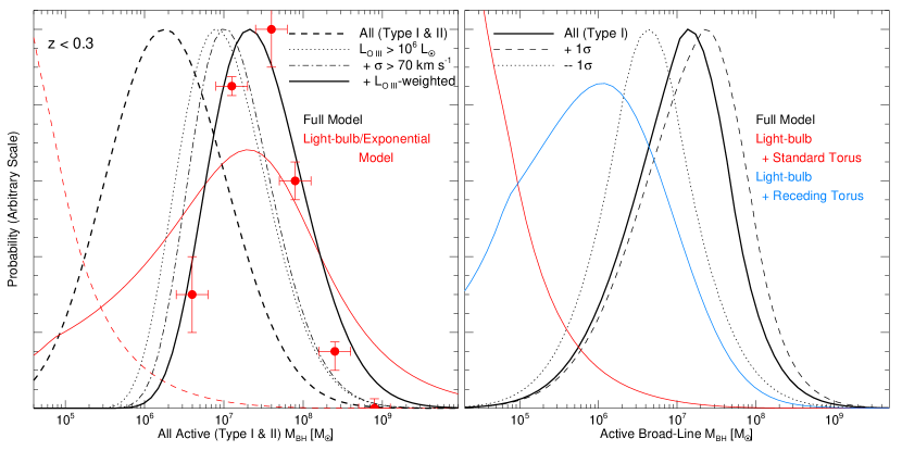
Figure 18.— Predicted distribution of currently active black hole masses, both considering all types (Type I & II; left) and only those visible as broad-line quasars (Type I; right), at low $z\lesssim 0.3$ redshift, from our $\dot{n}(L_{\rm peak})$ distribution and the estimation of the “broad-line” phase directly from the simulations. In the left panel (all quasar types), we consider the result with arbitrarily faint luminosity limits (dashed line), and with the luminosity completeness limit (dotted) and both luminosity limit and velocity dispersion limit (dash-dot) of the SDSS sample of Heckman et al. (2004). We then consider the mass distribution with these limits, weighted by OIII luminosity, for direct comparison to the mass function of Heckman et al. (2004), shown as red circles (vertical errors represent the range in different parameterizations of the luminosity-weighted mass function from Heckman et al. (2004), their Fig. 1, horizontal errors a $\sim 0.2$ dex uncertainty in the black hole mass). Black lines show this for our full model, red lines show the full distribution (dashed) and distribution with the same weighting and selection effects as Heckman et al. (2004) (solid) for a light-bulb or exponential light curve model of quasar evolution. At right, the distribution of active “broad-line” quasar masses (solid, where an object is a “broad-line” quasar if the observed quasar B-band luminosity is above a factor $f_{\rm BL}=1$ of that of the host galaxy – dotted and dashed lines show the result if $f_{\rm BL}=0.3$ or 3, respectively). Black lines show the prediction of the full model, red and blue lines the predictions of a light-bulb/exponential light curve model with a standard torus model (red) and receding torus model (blue) used to determine the broad-line fraction.

Our predicted $n(M_{\rm BH})$, i.e. the number of observed active quasars at low redshift in a logarithmic interval of black hole mass, is shown in Figure 18. We consider the complete distribution of active quasar masses, for both broad-line and non broad-line objects, in the left panel of the figure, and the distribution of broad-line objects only, $n(M^{\rm BL}_{\rm BH})$, in the right panel. On the left, we show the complete distribution which would be observed without any observational limits (dashed line). We calculate this from the distributions of Eddington ratios in our simulations, as a function of current and peak luminosity, and our fit to $\dot{n}(L_{\rm peak})$ (as, e.g. for our Monte Carlo realizations). We also consider the observed distribution if we apply the luminosity limit for completeness from the SDSS sample of Heckman et al. (2004) (dotted), $L_{\rm[O\,III]}>10^{6}\,L_{\sun}$, which using their bolometric corrections yields $L>3.5\times 10^{9}\,L_{\sun}$, and then additionally applying their minimum velocity dispersion $\sigma>70\,{\rm km\,s^{-1}}$ (dot-dashed). Finally, we can weight this distribution by luminosity (solid line) to compare directly to that determined in their Fig. 1. The red points are taken from the luminosity-weighted black hole mass function of Heckman et al. (2004), which serves as a rough estimate of the active black hole mass distribution given their selection effects. Vertical error bars represent the range in parameterizations of the mass function from Heckman et al. (2004), including whether or not star formation is corrected for and limiting the sample to luminosities $L\gtrsim 10^{10}\,L_{\sun}$ or Eddington ratios $>0.01$. Horizontal errors represent an uncertainty of $0.2\,$dex in the black hole mass estimation (representative of uncertainties in the $M_{\rm BH}-\sigma$ relation used). The agreement is good, especially given the significant effects of the selection criteria and luminosity-weighting.

We also consider the predictions of a “light-bulb” or “exponential / fixed Eddington ratio” model of the quasar lifetime for the active black hole mass distribution (red lines). For purposes of the active black hole mass function, the two predictions are identical and independent of the assumed quasar lifetime (modulo the arbitrary normalization), as both assume that all observed quasars are accreting at a fixed Eddington ratio, giving the distribution of active black hole masses. The dashed line shows the prediction for the complete active black hole mass function, which rises sharply to lower luminosities, as it must given a luminosity function which increases monotonically to lower luminosities. The solid line shows the prediction of such a model with the complete set of selection effects from Heckman et al. (2004) described above applied, as with the solid black line showing the prediction of our modeling. Here, we chose the characteristic Eddington ratio $\approx 1.0$ by fitting the predicted curve to the Heckman et al. (2004) observations. Note that both the characteristic Eddington ratio and lifetime (normalization) of the curve are fitted, so the relative normalization of this curve and our full model prediction are not the same; for example, the predicted total absolute number of active $M_{\rm BH}>10^{9}$ quasars is higher in the full model than in the light-bulb or exponential models. Still, it is clear that these models produce too broad a distribution of active black hole masses, in disagreement with the observations. We could, of course, obtain an arbitrarily close agreement with the observations if we fit to the distribution of accretion rates, but such a model would recover a quasar lifetime and accretion rate distribution quite similar to ours, as is evident from the agreement between the predictions of our simulations and the observations. A purely empirical model of this type is considered by e.g. Merloni (2004), who finds that similar qualitative evolution in the quasar lifetime and anti-hierarchical black hole assembly to that predicted by our modeling is implied by the combination of quasar luminosity functions and the black hole mass function.

On the right of the figure, we show our predicted mass distribution for low-redshift, active “broad-line” quasars (solid black lines), where we estimate that an object is a “broad-line” quasar if the observed quasar B-band luminosity is above a factor $f_{\rm BL}=1$ of that of the host galaxy – dotted and dashed lines show the result if $f_{\rm BL}=0.3$ or 3, respectively, parameterizing the range of different observed samples. As discussed above, the range of $f_{\rm BL}$ shown can be, alternatively, thought of as a parameterization of uncertainty in the host galaxy gas fraction, if (in an observed sample), the sensitivity to seeing quasar broad lines against host galaxy contamination is known. Therefore, the location of the peak in the active broad-line black hole mass function can be used, just as the mean broad line fraction vs. luminosity, as a test of the typical gas fractions of bright quasar host galaxies, and can constrain potential evolution in these gas fractions with redshift.

The prediction shown is testable, but appears to be in good agreement with preliminary results for the distribution of active broad-line black hole masses from the SDSS (e.g., McLure & Dunlop, 2004). The observations may show fewer low-mass black holes than we predict, but this is expected, as observed samples are likely incomplete at the low luminosities of these objects (even at the Eddington limit, a $10^{5}\,M_{\sun}$ black hole has magnitude $M_{g}\sim-16$). If, in our model, we were to consider instead a standard torus scenario for the definition of the broad-line phase, we would predict the same curve as that shown in the left half of the figure (black dashed; our prediction for the cumulative active black hole mass function). This is because the standard torus model predicts that a constant fraction of objects are broad-line quasars, regardless of mass or luminosity, thus giving identical distributions of Type I and Type II quasar masses. If we consider a luminosity-dependent or receding torus model, the prediction is nearly identical to the black line shown. This is because, as shown in Figure 16, our prediction for the broad line fraction as a function of luminosity is similar to that of the receding torus model. The differences in the model predictions for the broad-line fraction as a function of luminosity do manifest in the prediction for the active broad-line black hole mass function, but the difference in these models is smaller than the $\sim 1\sigma$ range from different values of $f_{\rm BL}$ shown. However, if we consider different models for the quasar light curve or lifetime, the predicted active broad-line mass function is quite different (as is the cumulative active black hole mass function).

We show the predictions of a light-bulb or exponential light curve model for quasar evolution in the figure, adopting either a standard torus model (red) or receding torus model (blue) to determine the broad-line fraction as a function of luminosity. For the standard torus model, this predicts that the broad line mass function should trace the observed luminosity function, rising monotonically to lower black hole masses in power-law fashion (just as seen in the red dashed line in the left half of the figure for the cumulative black hole mass function). For the receding torus model, the active black hole mass function shows a peak (because, at lower luminosities, there are more observed quasars, but a larger fraction of them are obscured). However, the location of this peak is at roughly an order of magnitude smaller black hole mass than for our prediction. This assumes a typical Eddington ratio $\sim 1$, which we have fitted to the cumulative black hole mass function – the peak in the broad-line active black hole mass function in these models could be shifted to larger black hole masses by assuming a smaller typical Eddington ratio, but this would only worsen the agreement with the cumulative black hole mass function of Heckman et al. (2004). Furthermore, a robust difference between the models is that the light bulb or Eddington-limited/exponential models predict, for the standard torus case, no turnover in the active broad-line black hole mass function, and for the receding torus case, a broader distribution in active broad-line quasar black hole masses than is predicted in our modeling. Roughly, the lognormal width of this distribution in our model is $\sim 0.6$ dex, whereas the light-bulb or exponential light curve models have a distribution with width $\sim 1.0$ dex. As noted above, we obtain a similar prediction if we adopt our full obscuration model instead of the receding torus model here. A determination of the range of active, broad-line quasar masses can, therefore, constrain quasar lifetimes and light curves.

Our model makes an accurate prediction for the distribution of active black hole masses, even at $z\sim 0$ where our extrapolation of the luminosity function is uncertain. It is important to distinguish this from the predicted relic black hole mass distribution, derived in § 6, which must account for all quasars, i.e. $\dot{n}(L_{\rm peak})$ integrated over redshift. We additionally find for broad-line quasars, as we expect from our prediction of the broad-line phase, that these objects are primarily radiating at large Eddington ratios, $l\sim 0.2-1$, but we address this in more detail in § 5. The success of this prediction serves not only to support our model, but also implies that we can extrapolate to fairly low luminosities, even bright Seyfert systems at $z\sim 0$. This suggests that many of these systems, at least at the bright end, may be related to our assumed quasar evolution model, fueled by similar mechanisms and either exhibiting weak interactions among galaxies or relaxing from an earlier, brighter stage in their evolution. As we speculate in § 8, our description of self-regulated black hole growth may also be relevant to fainter Seyferts, even those that reside in apparently undisturbed galaxies.

5. The Distribution of Eddington Ratios

In traditional models of quasar lifetimes and light curves, the Eddington ratio, $l\equiv L/L_{\rm Edd}$ is generally assumed to be constant. Even complex models of the quasar population which allow for a wide range of Eddington ratios according to some probability distribution $P(l)$ implicitly associate a fixed Eddington ratio with each individual quasar, and do not allow for $P(l)$ to depend on instantaneous luminosity or host system properties. However, this is a misleading assumption in the context of our model, as the Eddington ratio varies in a complicated manner over most of the quasar light curve. Furthermore, the integrated time at a given Eddington ratio is different in different systems, with more massive, higher peak luminosity systems spending more time at large ($l\sim 1$) Eddington ratios.

The probability of being at a given Eddington ratio should properly be thought of as a conditional joint distribution $P(l\,|\,L,\,L_{\rm peak})$ in both instantaneous and peak luminosity, just as the quasar “lifetime” is more properly a conditional distribution $t_{Q}(L\,|\,L_{\rm peak})$. Rather than adopting a uniform Eddington ratio or Eddington ratio distribution, empirical estimates must consider more detailed formulations such as the framework presented in Steed & Weinberg (2003), which allows for a conditional bivariate Eddington ratio distribution and can therefore incorporate these physically motivated dependencies and complications in de-convolving observations of the quasar luminosity function to determine e.g. Eddington ratio distributions, active black hole mass functions, and other physical quantities.

Figure 19.— Distribution of Eddington ratios (left panels) and instantaneous black hole mass (right panels) as a function of quasar bolometric luminosity for our fiducial Milky Way-like A3 simulation, with $V_{\rm vir}=160\,{\rm km\,s^{-1}}$ and $L_{\rm peak}\sim 5\times 10^{13}\,L_{\sun}$. The trend of an increasingly narrow Eddington ratio and mass distribution (concentrated at higher values) with increasing luminosity is clear. The result of applying an ADAF-type radiative efficiency correction at low accretion rates is shown (dashed) as well as the result of considering only times after the final merger, with $M_{\rm BH}\sim M^{f}_{\rm BH}$ (dotted).

Figure 19 shows the distribution of Eddington ratios as a function of luminosity for the fiducial, Milky Way-like A3 simulation ($V_{\rm vir}=160\,{\rm km\,s^{-1}}$). Over the course of the simulation, the system spends a roughly comparable amount of time at a wide range of Eddington ratios from $l\sim 0.001-1$. At high luminosities, $L>10^{12}\,L_{\sun}$ for a system with $L_{\rm peak}\approx 10^{13}\,L_{\sun}$, the range of Eddington ratios, is concentrated at high values $l\sim 0.5-1$ with some time spent at ratios as low as $l\sim 0.1$. Note, however, that the y-axis of the plot is scaled logarithmically, so the time spent at $l\sim 0.1$ in this luminosity interval is a factor $\sim 5$ smaller than the time spent at $l\gtrsim 0.5$. Considering lower luminosities $10^{11}\,L_{\sun}<L<10^{12}\,L_{\sun}$, the distribution of Eddington ratios broadens down to $l\sim 0.01$. Going to lower luminosities still, $L<10^{11}\,L_{\sun}$, the distribution broadens further, with comparable time spent at ratios as low as $l\sim 0.001$, and becomes somewhat bimodal. At large luminosities near $L_{\rm peak}$, the system is primarily in Eddington-limited or near-Eddington growth. However, as we consider lower luminosities, we include both early times when the black hole is growing efficiently (high $l$) and late or intermediate times when the black hole is more massive but the accretion rate falls (low $l$). As we go to lower luminosities, the total time spent in sub-Eddington states increasingly dominates the time spent at $l\sim 1$, although the time spent at any given value of $l$ is fairly flat with $\log(l)$.

Roughly, at some luminosity $L$, there is a constant probability of being in some logarithmic interval in $l$,

$$P(l|L,L_{\rm peak})\sim\left[\log\Bigl{(}\frac{L_{\rm peak}}{L}\Bigr{)}\right]^{-1},\ \frac{L}{L_{\rm peak}}<l<1,$$ (30)

and $P(l|L,L_{\rm peak})=0$ otherwise. This is especially clear if we compare the distribution of Eddington ratios in each luminosity range obtained if we consider only times after the final merger of the black holes (dotted histograms). At the highest luminosities, the distribution is identical to that obtained previously, since all the time at these luminosities is during the final merger. However, as we move to lower luminosities, the characteristic $l$ move systematically lower, as we are seeing only the relaxation after the final “blowout” near $L_{\rm peak}$, with characteristic Eddington ratio $l=L/L_{\rm peak}$ at any given luminosity $L$. These trends are also clear if we consider the distribution of instantaneous black hole masses in each luminosity interval shown in the figure, which is trivially related to the Eddington ratio distribution at a given luminosity $L$ as

$$M_{\rm BH}=M_{0}\,\frac{L}{l\,L_{\rm Edd}(M_{0})}=\frac{L\,t_{S}}{l\,\epsilon_{r}c^{2}}.$$ (31)

Of course, it is clear here that $M_{\rm BH}\approx M^{f}_{\rm BH}=3\times 10^{8}\,M_{\sun}$ if we consider only times after the final merger.

It has also been argued from observations of stellar black hole binaries that a transition between accretion states occurs at a critical Eddington ratio $\dot{m}\equiv\dot{M}/\dot{M_{\rm Edd}}$, from radiatively inefficient accretion flows at low accretion rates (e.g., Esin, McClintock, & Narayan, 1997) to radiatively efficient accretion through a standard Shakura & Sunyaev (1973) disk. Although the critical Eddington ratio for supermassive black holes is uncertain, observations of black hole binaries (Maccarone, 2003) as well as theoretical extensions of accretion models (e.g., Meyer, Liu, & Meyer-Hofmeister, 2000) suggest $\dot{m}_{\rm crit}\sim 0.01$. We can examine whether this has a large impact on our predictions for the luminosity function and $\dot{n}(L_{\rm peak})$ distribution, by determining whether the distribution of Eddington ratios is significantly changed by such a correction. Because we assume a constant radiative efficiency $L=\epsilon_{r}\,\dot{M}\,c^{2}$ with $\epsilon_{r}=0.1$, we account for this effect by multiplying the simulation luminosity at all times by an additional “efficiency factor” $f_{\rm eff}$ which depends on the Eddington ratio $l=L/L_{\rm Edd}$,

$$f_{\rm eff}=\left\{\begin{array}[]{ll}1&\mathrm{if\ }l>0.01\\ 100\,l&\mathrm{if\ }l\leq 0.01.\end{array}\right.$$ (32)

This choice for the efficiency factor follows from ADAF models (Narayan & Yi, 1995) and ensures that the radiative efficiency is continuous at the critical Eddington ratio $l_{\rm crit}=0.01$. Applying this correction and then examining the distribution of Eddington ratios as a function of luminosity (dashed histograms in Figure 19), we see that the distribution of Eddington ratios is essentially identical, with only a slightly higher probability of observing extremely low Eddington ratios $l\lesssim 0.001$. Of course, our modeling of accretion processes does not allow us to accurately describe ADAF-like accretion at these low Eddington ratios, but such low values are not relevant for the observed luminosity functions and quantities with which we make our comparisons. This implies that such a transition in the radiative efficiency with accretion rate should not alter our conclusions regarding the luminosity function and the $\dot{n}(L_{\rm peak})$ distribution (essentially, the corrections are important only at luminosities well below those relevant in constructing the observed luminosity functions; see also Hopkins et al. 2005c for a calculation of the effects of such a correction on the fitted quasar lifetime and $\dot{n}(L_{\rm peak})$ distributions, which leads to the same conclusion).

Despite the broad range of Eddington ratios in the simulations, this entire distribution is unlikely to be observable in many samples. The effect of this can be predicted based on the behavior seen in Figure 19. For example, we consider the distribution of Eddington ratios that would be observed if the B-band luminosity $L_{B,{\rm obs}}\geq 10^{11}\,L_{\sun}$, comparable to the selection limits at high redshift of many optical quasar samples. As expected from the change in $l$ with luminosity, this restricts the observed range of Eddington ratios to large values $l\sim 0.1-1$, in good agreement with the range of Eddington ratios actually observed in such samples. Essentially, it has reduced the observed range to a bolometric luminosity $L\gtrsim 10^{12}\,L_{\sun}$ in the case shown, giving a similar distribution to that seen in the lower panel of the figure.

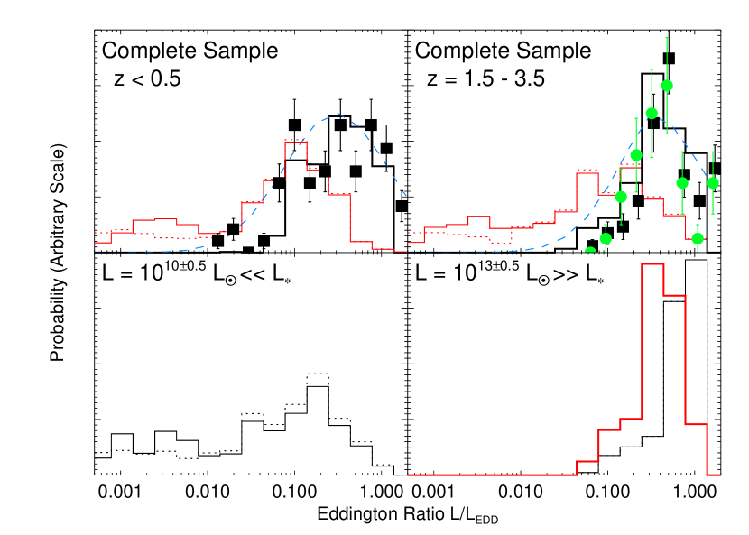
Figure 20.— Predicted distribution of Eddington ratios based on the luminosity function and the quasar evolution in our simulations, in two redshift intervals $z<0.5$ (upper left) and $1.5<z<3.5$ (upper right). The observed distributions for radio loud (black squares) and radio quiet (green circles) quasars are shown from Vestergaard (2004) with Poisson errors. Thick black lines show the predicted distribution given the same minimum observed luminosity as the observed sample. Thin red lines show the predicted distributions for a sample extending to arbitrarily faint luminosities, dotted lines show the same, with the ADAF correction of § 5 applied at low accretion rates. Blue dashed lines show the prediction for a fixed (luminosity-independent) Eddington ratio distribution in a light-bulb or exponential light curve model, fitted to the $z<0.5$ data and used to predict the $1.5<z<3.5$ Eddington ratio distribution given the observational luminosity limit. Lower panels show the predicted distributions for $z\lesssim 1$ in two luminosity intervals, above and below the “break” luminosity in the observed luminosity function (red lines here correspond to an observed (attenuated) B-band luminosity $L_{B,{\rm obs}}>10^{11}\,L_{\sun}$).

We compare our predicted distribution of Eddington ratios to observations in Figure 20. Using the distribution of peak luminosities $\dot{n}(L_{\rm peak})$ determined from the luminosity function, we can integrate over all luminosities to infer the observed Eddington ratio distribution,

$$P(l) \propto \int{{\rm d}\log L}\int{{\rm d}\log L_{\rm peak}}$$ (33)

$$\times P(l|L,L_{\rm peak})\,\frac{{\rm d}t(L,L_{\rm peak})}{{\rm d}\log L}\dot{n}(L_{\rm peak}).$$

As our estimate of $P(l|L,L_{\rm peak})$ above is rough, we do this by binning in $L_{\rm peak}$ and averaging the binned $P(l|L,L_{\rm peak})\,{\rm d}t/{\rm d}\log{L}$ for each simulation in the range of $L_{\rm peak}$, then weighting by $\dot{n}(L_{\rm peak})$ and integrating. We consider both the entire distribution that would be observed in the absence of selection effects (red histograms), and the distribution observed demanding a B-band luminosity above some reference value, $L_{B,{\rm obs}}>L_{\rm min}$ (black histograms). The results are shown for redshifts $z<0.5$ and $z=1.5-3.5$, along with the observed distribution from Vestergaard (2004), with assumed Poisson errors. The observations should be compared to the black histograms, which have luminosity thresholds $L=10^{10}\,L_{\sun}\ {\rm and}\ 10^{11}\,L_{\sun}$ for $z<0.5$ and $z=1.5-3.5$, respectively, corresponding approximately to the minimum observable luminosities in the observed samples in each redshift interval.

The agreement is good, given the observational uncertainties, and it suggests that the observed Eddington ratio distribution can be related to the non-trivial nature of quasar lifetimes and light curves we model, rather than some arbitrary distribution of fixed $l$ across sources. However, the selection effects in the observed samples are quite significant – the complete distribution of Eddington ratios is similar in both samples, implying that the difference in the observed Eddington ratio distribution is primarily a consequence of the higher luminosity limit in the observed samples – and a more detailed test of this prediction requires fainter samples.

Still, there is a systematic offset in the observed samples at $z<0.5$ and $z=1.5-3.5$ which does not owe to selection effects. At progressively lower redshifts, more quasars with luminosities further below the “break” in the luminosity function are observed, and therefore the observed Eddington ratio is broadened to lower Eddington ratios $l\sim 0.1$, whereas at high redshift the distribution is more peaked at slightly higher Eddington ratios. This difference, although not dramatic, is a prediction of our model not captured in “light bulb” or “fixed Eddington ratio” models, even when allowing for a distribution of Eddington ratios, if such a distribution is static. We demonstrate this by fitting the low-redshift Eddington ratio distribution to a Gaussian (blue dashed lines in upper left), and then assuming that this distribution of accretion rates is unchanged with redshift, giving (after applying the same selection effects which yield the black histograms plotted) the blue dashed line in the upper right panel. Although the agreement may appear reasonable, the difference is significant – such a fit overpredicts the fraction of high redshift objects at Eddington ratios $\lesssim 0.1$ and underpredicts the fraction at $\sim 0.3$, giving a somewhat poor fit overall ($\chi^{2}/\nu=2.7$, but with typical $\gtrsim 3\sigma$ overpredictions for Eddington ratios $\lesssim 0.1$).

Furthermore, without being modified to allow for a distribution of Eddington ratios, such models are clearly inconsistent with the observations, as they would predict a single, constant Eddington ratio. However, models which fit the observed evolution in the quasar luminosity function with a non-static distribution of accretion rates do recover the broadening of the Eddington ratio distribution at low redshift, so long as strong evolution in the distribution of accretion rates for systems of a given black hole mass is not allowed (Steed & Weinberg, 2003), giving a qualitatively similar picture of the evolution we model. Regardless of the evolution in accretion rates, an advantage of our modeling is that it provides a physically motivated predicted distribution of accretion rates, as opposed to being forced to adopt the distribution of accretion rates from observational input (which can be, as demonstrated in the figure, significantly biased by observational selection effects). The dotted histograms show the distribution if we apply our ADAF correction to the intrinsic distribution, and demonstrate that this does not significantly change the result. We note that our model for black hole accretion employs the Eddington limit as a maximum accretion rate; if we remove this restriction, we find that the simulations spend some small but non-negligible time with $l\sim 1-2$, which is also consistent with the observations.

Furthermore, we can make a prediction of this model which can be falsified, namely that the Eddington ratio distribution at luminosities well below the break in the luminosity function should be broader and extend to lower values than the distribution at luminosities above the break luminosity. We quantify this in the lower panels of Figure 20, for the distribution at low redshifts $z\lesssim 1$. Here we consider two bins in luminosity, $L=10^{9.5}-10^{10.5}\,L_{\sun}$ and $L=10^{12.5}-10^{13.5}\,L_{\sun}$, for redshifts where the break in the luminosity function is at approximately $L\sim 10^{11}-10^{12}\,L_{\sun}$. Clearly, the distribution is broader and extends to lower Eddington ratios in the former luminosity interval, whereas in the latter it is strongly peaked about $l\sim 0.2-1$, for both the complete distribution (black) and that with $L_{B,{\rm obs}}\geq 10^{11}\,L_{\sun}$ (red). The distribution obtained applying the ADAF correction described above is shown as dotted histograms. Despite the fact that the Eddington ratio distribution at low luminosities will be strongly biased by selection effects, a reasonably complete sample should be able to test this prediction, at least qualitatively.

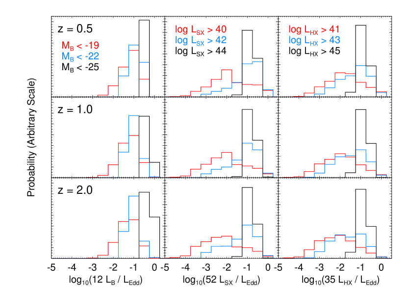
Figure 21.— Predicted distribution of Eddington ratios based on the luminosity function and the quasar evolution in our simulations, at three redshifts $z=0.5$ (top panels), $z=1.0$ (middle), and $z=2.0$ (bottom). The inferred distribution of Eddington ratios, adopting a constant bolometric correction from the observed (attenuated) luminosity in each of three bands is shown, i.e. assuming $L=12\,L_{B}^{\rm obs}$ ($4400\,$Å; left), $L=52\,L_{SX}^{\rm obs}$ (0.5-2 keV; middle), and $L=35\,L_{HX}^{\rm obs}$ (2-10 keV; right). For each waveband, results are shown for three reference luminosities. In B-band, $M_{B}<-19$ (red), $M_{B}<-22$ (blue), and $M_{B}<-25$ (black). In soft X-rays, $\log(L_{SX}[{\rm erg\,s^{-1}}])>40\ (\rm red),\ 42\ (\rm blue),\ 44\ (\rm black)$. In hard X-rays, $\log(L_{HX}[{\rm erg\,s^{-1}}])>41\ (\rm red),\ 43\ (\rm blue),\ 45\ (\rm black)$.

We illustrate the effects of changing observed waveband, redshift, and luminosity thresholds on the observed Eddington ratio distribution in Figure 21. Here, we plot the predicted distribution of Eddington ratios determined as in Figure 20, from our fitted $\dot{n}(L_{\rm peak})$ distribution at each redshift and the distribution of Eddington ratios as a function of instantaneous and peak luminosity in each of our simulations (specifically, these are drawn from the Monte Carlo realizations of the quasar population described in § 8). We show the predictions at three redshifts $z=0.5$ (top panels), $z=1.0$ (middle), and $z=2.0$ (bottom). For each redshift, results are shown in three wavebands, and with three reference luminosities. In B-band, we require $M_{B}<-19$ (red), $M_{B}<-22$ (blue), and $M_{B}<-25$ (black). In soft X-rays, $\log(L_{SX}[{\rm erg\,s^{-1}}])>40\ (\rm red),\ 42\ (\rm blue),\ 44\ (\rm black)$. In hard X-rays, $\log(L_{HX}[{\rm erg\,s^{-1}}])>41\ (\rm red),\ 43\ (\rm blue),\ 45\ (\rm black)$. The observationally inferred distribution of Eddington ratios at each redshift is loosely estimated by adopting a constant bolometric correction from the observed (attenuated) luminosity in each of three bands shown, i.e. assuming $L=12\,L_{B}^{\rm obs}$ ($4400\,$Å; left), $L=52\,L_{SX}^{\rm obs}$ (0.5-2 keV; middle), and $L=35\,L_{HX}^{\rm obs}$ (2-10 keV; right). This follows common practice in many observational estimates of the Eddington ratio distribution and allows for the effects of attenuation, but we caution that it can be misleading.

If we instead use the luminosity-dependent bolometric corrections of Marconi et al. (2004) which we adopt throughout, even given that we are calculating from the observed (attenuated) luminosities, we do not see the large population of highly sub-Eddington (Eddington ratios $\lesssim 10^{-3}$) quasars in soft and hard X-ray samples with low luminosity thresholds. This is because these are actually reasonably high-Eddington ratio quasars, but our bolometric corrections imply that a larger fraction of the bolometric luminosity is radiated in the X-ray at low bolometric luminosity, meaning that assuming a constant bolometric correction will underestimate the Eddington ratios of high-bolometric luminosity sources. Regardless, the figure illustrates both the importance of different wavelengths (i.e. the ability to observe more low-Eddington ratio sources in X-ray as compared to optical samples) and luminosity/magnitude limits on the inferred distribution of Eddington ratios. For example, even for relatively deep B-band quasar samples complete to $M_{B}<-23$ (i.e. complete to essentially all objects traditionally classified as having “quasar-like” luminosities), the expected observed Eddington ratio distribution at $z\sim 0.5-2$ is quite sharply peaked about $\sim 0.1-0.3$, in good agreement with recent observational results (Kollmeier et al., 2005).

We do not compare to the $z=0$ distribution of black hole accretion rates, as this is dominated by objects at extremely low Eddington ratios $l\sim 10^{-5}-10^{-4}$ (e.g., Ho, 2002; Marchesini et al., 2004; Jester, 2005), which are well below the range we model, and are not likely to be driven by merger activity (many of these objects are quiescent, low-luminosity Seyferts in normal spiral galaxy hosts); furthermore, many of these objects are not accreting at the Bondi rate (Fabian & Canizares, 1988; Blandford & Begelman, 1999; Di Matteo et al., 2000; Narayan et al., 2000; Quataert & Gruzinov, 2000; Di Matteo et al., 2001; Loewenstein et al., 2001; Bower et al., 2003), clearly showing that our simulations must incorporate more sophisticated models for accretion in quiescent, low-luminosity states (when gravitational torques cannot provide a mechanism to drive large amounts of gas to the central regions of the galaxy) in order to describe such phases.

However, it has been suggested that the rapid “blowout” phase and subsequent decay in accretion rates seen in our simulations, coupled with spectral modeling of radiatively inefficient accretion modes, can explain the apparently bimodal distribution of low-redshift accretion rates (Cao & Xu, 2005). Moreover, present-day, relaxed ellipticals are observed to have mass accretion rates $\sim 10^{-4}$ implying a long relaxation time at moderate and low accretion rates, qualitatively similar to that seen after the “blowout” in our modeling (Hopkins et al. 2005f). A pure exponential decay in accretion rate after the peak quasar phase would give $\dot{m}=\dot{M}/\dot{M}_{\rm Edd}\sim\exp{(-t_{H}/t_{Q})}$ at present, where $t_{H}$ is the Hubble time and $t_{Q}$ is the quasar lifetime of order e.g. the Salpeter time $t_{S}=4\times 10^{7}$ yr, yielding an unreasonably low expected accretion rate $\dot{m}\sim 10^{-145}$. Even assuming an order of magnitude larger quasar lifetime, this gives $\dot{m}\sim 10^{-15}$, far below observed values, implying that regardless of the fueling mechanisms at low luminosities, the basic key point of our modeling must be true to some extent, namely that quasars spend long times relaxing at moderate to low Eddington ratios.

6. The Mass Function of Relic Supermassive Black Holes from Quasars

From the $M_{\rm BH}$-$\sigma$ relation and other host galaxy-black hole scalings, estimates of bulge and spheroid velocity dispersions have been used to determine the total mass density ($\rho_{\rm BH}$) and mass distribution of local, primarily inactive supermassive black holes (e.g., Salucci et al., 1999; Marconi & Salvati, 2002; Yu & Tremaine, 2002; Ferrarese, 2002; Aller & Richstone, 2002; Marconi et al., 2004; Shankar et al., 2004). These estimates, along with others based on X-ray background synthesis (e.g., Fabian & Iwasawa, 1999; Elvis et al., 2002), have compared these quantities to those expected based on the mass distribution of ‘relic’ black holes grown in quasars. It appears that most, and perhaps nearly all of the present-day black hole mass density was accumulated in bright quasar phases, and the $M_{\rm BH}-\sigma$ and $M_{\rm BH}-L_{\rm bulge}$ correlations yield estimates of the local mass function in good agreement with those from hard X-ray AGN luminosity functions (Marconi et al., 2004).

However, this modeling is dependent on several assumptions. Namely, the average radiative efficiency $\epsilon_{r}$, Eddington ratio $l$, and average quasar lifetime $t_{Q}$ are generally taken to be constants and either input into the model or constrained by demanding agreement with the local mass function. In our simulations, we find the quasar lifetime and Eddington ratio to be complex functions of both luminosity and host system properties (as opposed to being constants). We also find that quasars spend a large fraction of their lives in obscured growth phases, suggesting some mass gain outside of the bright quasar phase. It is thus of interest to determine the relic black hole mass function expected from our model for quasar evolution.

Using our estimate for the birthrate of quasars with a given peak luminosity at a particular redshift, $\dot{n}(L_{\rm peak})$, obtained from the luminosity function in § 3.2, we can estimate the total number density of relic quasars accumulated by a particular redshift that were born with a given $L_{\rm peak}$ (per logarithmic interval in $L_{\rm peak}$) from

$$n(L_{\rm peak})=\int{\,\dot{n}(L_{\rm peak})\,{\rm d}t}=\int{\frac{\dot{n}(L_{\rm peak},z)\,{\rm d}z}{(1+z)H(z)}}.$$ (34)

By redshift $z=0$, most of these quasars will be “dead,” with only a small residual fraction having been activated in the recent past.

Using our log-normal form for $\dot{n}(L_{\rm peak})$, with normalization $\dot{n}_{\ast}$ and dispersion $\sigma_{\ast}$ held constant and only the median $L_{\ast}=L_{\ast}^{0}\,\exp{(k_{L}\tau)}$ evolving with redshift, this integral can be evaluated numerically to give the space density of relic quasars $n(L_{\rm peak})$. Finally, we use $M^{f}_{\rm BH}(L_{\rm peak})$, roughly the Eddington mass of the given peak luminosity (but determined more precisely in § 2.4) to convert from ${\rm d}n(L_{\rm peak})/{\rm d}\log L_{\rm peak}$ to ${\rm d}n(M_{\rm BH})/{\rm d}\log M_{\rm BH}$. This formulation implicitly assumes that black holes do not undergo subsequent mergers after the initial quasar-producing event. However, this effect should be small (a factor $\lesssim 2$) as subsequent mergers would be dry (gas poor). We explicitly calculate the effects of dry mergers on the spheroid mass function (essentially a rescaling of the black hole mass function calculated here) in Hopkins et al. (2005e), and show that this is a small effect (significantly less than the uncertainties owing to our fit to the quasar luminosity function) even assuming the maximum dry merger rates of e.g. van Dokkum (2005).

This mass function can then be integrated over $dM_{\rm BH}$ to give the total present-day black hole mass density, $\rho_{\rm BH}$. Neglecting temporarily the small corrections to $M^{f}_{\rm BH}(L_{\rm peak})$ from § 2.4, we expect

$$M^{f}_{\rm BH}\approx M_{\rm Edd}(L_{\rm peak})=\frac{L_{\rm peak}\,t_{S}}{\epsilon_{r}c^{2}}$$ (35)

where $t_{S}/\epsilon_{r}c^{2}\approx 2.95\times 10^{-5}\,M_{\sun}/L_{\sun}$, so therefore,

$$\rho_{\rm BH}=\frac{t_{S}}{\epsilon_{r}c^{2}}\int{L_{\rm peak}\,n(L_{\rm peak})\,{\rm d}\log L_{\rm peak}}.$$ (36)

This can be combined with the integral over redshift for $n(L_{\rm peak})$, giving, at each $z$, a pure Gaussian integral over $\log{(L_{\rm peak})}$, in the form

$$\rho_{\rm BH} = \frac{L_{\ast}^{0}\,t_{S}}{\epsilon_{r}c^{2}}\frac{\dot{n}_{\ast}}{H_{0}}\,e^{\frac{1}{2}(\sigma_{\ast}\ln{10})^{2}}\,\int{\frac{e^{k_{L}\tau}\,dz}{(1+z)\,\hat{H}(z)}}$$ (37)

$$= \frac{L_{\ast}^{0}\,t_{S}}{k_{L}\epsilon_{r}c^{2}}\frac{\dot{n}_{\ast}}{H_{0}}\,e^{\frac{1}{2}(\sigma_{\ast}\ln{10})^{2}}\,\Bigl{(}e^{k_{L}\tau_{f}}-e^{k_{L}\tau}\Bigr{)},$$

where $\hat{H}(z)\equiv H(z)/H_{0}$ and $\tau_{f}$ is the fractional lookback time at some upper limit. We must modify this integral above $z\sim 2$ to account for the decreasing space density of bright quasars, applying either our density or peak-luminosity evolution turnover from § 3.2, but quasars at these high redshifts contribute only a small fraction to the present-day density. Thus, in this formulation, the evolution of the total supermassive black hole mass density, i.e. $\rho_{\rm BH}(z)/\rho_{\rm BH}(z=0)$, is given approximately by the dimensionless integral above, and depends only on how $L_{\ast}$ evolves, essentially the rate at which the break in the quasar luminosity function shifts. Although this is not strictly true if we include corrections to $M^{f}_{\rm BH}(L_{\rm peak})$ based on $L_{\rm peak}$, the difference is small and this behavior is essentially preserved. Note that the total supermassive black hole mass density is independent of corrections from subsequent dry mergers, which (being gas poor) conserve total black hole mass.

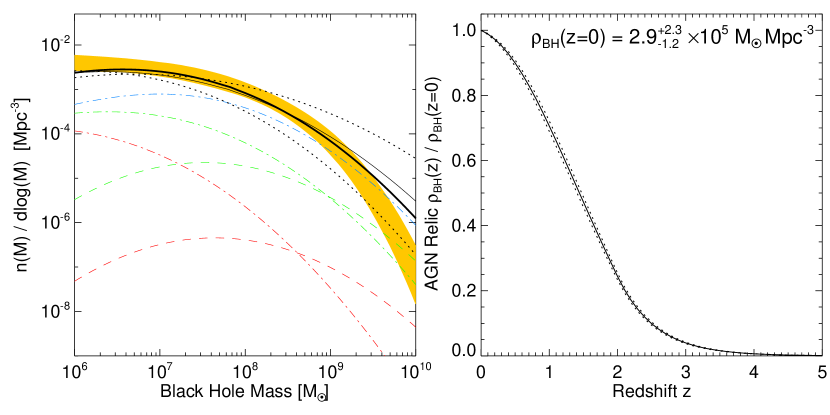
Figure 22.— Right: Total predicted quasar relic black hole mass density and evolution of the fractional black hole mass density with redshift. Dotted lines show the difference resulting from $1\sigma$ deviation in fitted $\dot{n}(L_{\rm peak})$ from the luminosity function. Left: Predicted present $z=0$ relic mass function (thick black line), for comparison with the $1\sigma$ range (yellow) of the inferred supermassive black hole mass function from Marconi et al. (2004). Also shown are the results given $1\sigma$ errors in the fitted $\dot{n}(L_{\rm peak})$ distribution (dotted lines), or ignoring the small corrections to $M^{f}_{\rm BH}(L_{\rm peak})$ from § 2.4 (thin black line). Dot-dashed lines show the predicted mass function at $z=1.5,\,3.0,\,5.0$ (blue, green, and red, respectively). The extensions to $z>2$ includes the turnover (pure peak luminosity evolution form) in the quasar space density above $z=2$ from high-redshift luminosity functions described in § 3.2, except for the dashed green and red lines which use the pure density evolution form.

Figure 22 shows our prediction for the mass distribution of supermassive black holes, as well as the total density $\rho_{\rm BH}$ and its evolution with redshift. We find a total relic black hole mass density of $\rho_{\rm BH}=2.9^{+2.3}_{-1.2}\times 10^{5}\,M_{\sun}\,{\rm Mpc^{-3}}$, in agreement with the observational estimate of $\rho_{\rm BH}=2.9\pm 0.5\,h^{2}_{0.7}\times 10^{5}\,M_{\sun}\,{\rm Mpc^{-3}}$, by Yu & Tremaine (2002) ($h_{0.7}\equiv H_{0}/70\,{\rm km\,s^{-1}\,Mpc^{-1}}$; their result is converted from $h=0.65$), and within $1\sigma$ of the value $\rho_{\rm BH}=4.6^{+1.9}_{-1.4}h^{2}_{0.7}\times 10^{5}\,M_{\sun}\,{\rm Mpc^{-3}}$, of Marconi et al. (2004), based on the observations of Marzke et al. (1994), Kochanek et al. (2001), Nakamura et al. (2003), Bernardi et al. (2003), and Sheth et al. (2003). The fractional evolution of $\rho_{\rm BH}$ with redshift is quite well constrained, and we find, as with previous estimates, that most of the present-day black hole mass density accumulates at moderate to low redshifts $z\approx 0.5-2.5$. The $1\sigma$ errors are shown as dotted lines in the figure, and are close to our best-fit estimate, as we have demonstrated that this quantity depends only on $k_{L}$, the rate of evolution of the break in the luminosity function with redshift, which is fairly well-constrained by observations (from our fitting to the luminosity functions, $k_{L}=5.61\pm 0.28$). The difference in $\rho_{\rm BH}$ if we include or neglect the small corrections to $M^{f}_{\rm BH}$ is negligible compared to our errors ($\sim 5\%$).

Our estimate for the relic black hole mass distribution (thick black line) also agrees well with observational estimates, with all observations within the range allowed by the $1\sigma$ errors of our fitting to the luminosity function (dotted lines). The observations shown are again from Marconi et al. (2004), based on the combination of observations by Marzke et al. (1994), Kochanek et al. (2001), Nakamura et al. (2003), Bernardi et al. (2003), and Sheth et al. (2003). The high mass end of the black hole mass function $M_{\rm BH}>10^{9}\,M_{\sun}$ is relatively sensitive to whether or not we apply the $M^{f}_{\rm BH}(L_{\rm peak})$ corrections of § 2.4, instead of taking $M^{f}_{\rm BH}=M_{\rm Edd}(L_{\rm peak})$ (thin line), as well as to our fitting procedure. However, the agreement is still good, and this is also where the observational estimates of the mass distribution are most uncertain, as they are generally extrapolated to these masses, and are sensitive to the assumed intrinsic dispersions in the $M_{\rm BH}-\sigma$ and $M_{\rm BH}-L_{\rm bulge}$ relations (Yu & Tremaine, 2002).

If, instead, we adopt a light-bulb, constant Eddington ratio, or exponential light curve model for quasar evolution, we would have $M_{\rm BH}^{f}\propto L_{\rm peak}$, and thus the prediction would be similar to the thin black line shown, a somewhat worse fit at high black hole masses. However, in these models this can be remedied by adjusting the typical Eddington ratios, quasar lifetimes, or radiative efficiencies. We do not show the range of predictions of these models for the relic supermassive black hole mass function, as they have been examined in detail previously (e.g., Salucci et al., 1999; Marconi & Salvati, 2002; Yu & Tremaine, 2002; Ferrarese, 2002; Aller & Richstone, 2002; Marconi et al., 2004; Shankar et al., 2004). These works demonstrate that the observed quasar luminosity functions are consistent with the relic supermassive black hole mass function, given typical radiative efficiencies $\epsilon_{r}\sim 0.1$ and Eddington ratios $\sim 0.5-1.0$, and that most of the mass of black holes is accumulated in bright, observed phases, or else the required radiative efficiency would violate theoretical limits.

That our model of quasar lifetimes and obscuration reproduces the observed $z=0$ supermassive black hole mass function explicitly demonstrates that we are consistent with these constraints. By choice, the radiative efficiency in our simulations is $\epsilon_{r}=0.1$, and accretion rates are not allowed to exceed Eddington. As noted in § 4, most of the black hole mass is accumulated and radiant energy released in the final, “blowout” phase of quasar evolution, and here our black hole mass function and cumulative black hole mass density demonstrate that our modeling is consistent with integrated energy and mass arguments such as that of Soltan (1982), despite the fact that quasars spend more time in obscured phases than they do in bright optical quasar phases. In fact, comparison of our predicted total black hole mass density with estimates from the $z=0$ black hole mass distribution allows some latitude for significant mass gain in radiatively inefficient growth or black holes in small, disky spheroids, although we emphasize that this is mainly because the uncertainty in our prediction is large, it is not inherent or necessary in our modeling.

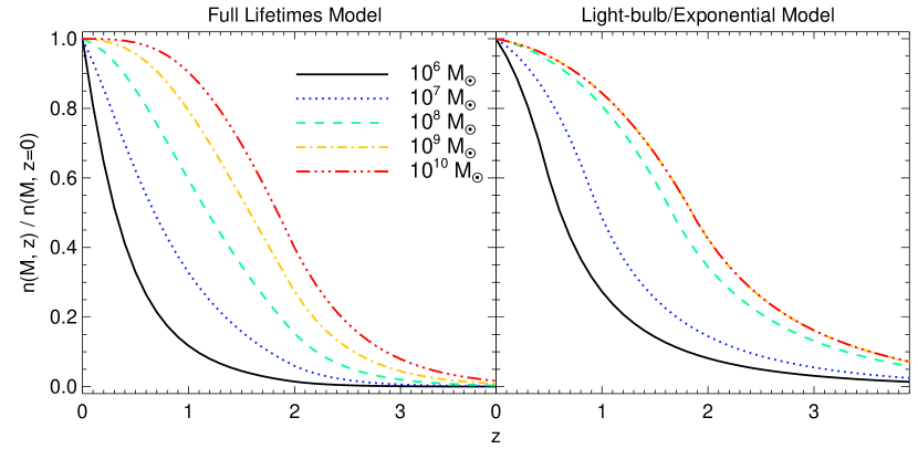
Figure 23.— Fractional number density $n(M,\,z)/n(M,\,z=0)$ of black holes of a given mass as a function of redshift, for several different black hole masses as shown. For $z>2$ this includes the turnover (pure density evolution form) in the quasar space density above $z=2$ from high-redshift luminosity functions described in § 3.2. Left panel shows the results using our full model of quasar lifetimes, right panel assuming a “light-bulb” or exponential (constant Eddington ratio) light curve model. The yellow dot-dash ($10^{9}\,M_{\sun}$) and red triple-dot-dash ($10^{10}\,M_{\sun}$) curves are nearly identical in the right panel.

The anti-hierarchical nature of black hole formation, where less massive black holes are formed at lower redshift, is reflected in our modeling by the shift of the break in the quasar luminosity function to lower values with decreasing redshift. This can be seen in Figure 22, where the black hole mass distributions are shown at redshifts $z=1.5,\,3.0\ {\rm and}\ 5.0$, assuming either pure peak luminosity evolution or pure density evolution for $z>2$ (dot-dashed and dashed, respectively). While the choice for the turnover in the $z>2$ quasar density matters little for the $z<2$ black hole mass functions, the low-$M_{\rm BH}$ distribution at high redshift (where observations do not constrain $\dot{n}(L_{\rm peak})$ well) is quite different between the two models. Figure 23 plots the fractional number density of black holes of a given mass as a function of redshift, i.e. $n(M,\,z)/n(M,\,z=0)$, where $n(M)={\rm d}n/{\rm d}\log{(M)}$ is just the number density at mass $M$. This figure demonstrates that higher-mass black holes originated over a larger range of redshifts, and that they mostly formed at higher redshift, compared to lower-mass black holes.

The right panel of Figure 23 compares our prediction to that of a light-bulb or exponential light curve model for quasar lifetimes. In these models, the anti-hierarchical nature of black hole assembly is dramatically suppressed. At the high-mass end, there is no measurable difference in the distribution of formation redshifts (i.e. the $M_{\rm BH}=10^{9}\,M_{\sun}$ and $M_{\rm BH}=10^{10}\,M_{\sun}$ curves are indistinguishable), and there is little change in the formation times at $M_{\rm BH}=10^{8}\,M_{\sun}$. The shift in formation redshift at lower masses, although significant, is smaller than that predicted in our model. If spheroids and black holes are produced together, as in our picture, these models of the quasar lifetime would imply that spheroids of masses $M_{\rm vir}\sim 10^{11}-10^{13}\,M_{\sun}$ all formed over nearly identical ranges of redshifts, which is inconsistent with many observations indicating anti-hierarchical growth of the red, elliptical galaxy population (e.g., Treu et al., 2001; van Dokkum et al., 2001; Treu et al., 2002; van Dokkum & Stanford, 2003; Gebhardt et al., 2003; Rusin et al., 2003; van de Ven et al., 2003; Wuyts et al., 2004; Treu et al., 2005; Holden et al., 2005; van der Wel et al., 2005; di Serego Alighieri et al., 2005; Nelan et al., 2005). Implications of our model for the red galaxy sequence are considered in Hopkins et al. (2005e), where we show that this weaker anti-hierarchical black hole (and correspondingly, spheroid) evolution is inconsistent with observed luminosity functions, color-magnitude relations, and mass-to-light ratios of elliptical galaxies.

Our modeling reproduces the observed total density and mass distribution of supermassive black holes at $z=0$ with black holes accreting at the canonical efficiency $\epsilon_{r}=0.1$ expected for efficient accretion through a Shakura & Sunyaev (1973) disk. Presumably, a large change in $\epsilon_{r}$ would give a significantly different relation between peak luminosity and black hole mass (for the same $L_{\rm peak}$, $M_{\rm BH}^{f}\propto 1/\epsilon_{r}$), and thus if the quasar lifetime remained similar as a function of peak luminosity, this would translate to a shift in the black hole mass function. The long obscured stage in black hole evolution does not generate problems in reproducing the black hole mass density, and the final phases of growth are still in bright optical quasar stages. However, a large Compton-thick population of black holes at all luminosities (or even at some range of luminosities at or above the break in the luminosity function) (e.g., Gilli et al., 2001; Ueda et al., 2003), or a large population accreting in a radiatively inefficient ADAF-type solution, as invoked to explain discrepancies in the X-ray background produced by synthesis models (Di Matteo et al., 1999), would result in a significant over-prediction of the present-day supermassive black hole density. As we demonstrate in § 7.2, invoking such populations is unnecessary, as our picture for quasar lifetimes and evolutionary obscuration self-consistently reproduces the observed X-ray background.

Finally, we note that we reproduce the $z=0$ distribution of black hole masses inferred from the distribution of spheroid velocity dispersions (Sheth et al., 2003) and luminosity functions (Marzke et al., 1994; Kochanek et al., 2001; Nakamura et al., 2003), based on the observed $M_{\rm BH}-\sigma$ relation and fundamental plane for galaxy properties (e.g., Bernardi et al., 2003; Gebhardt et al., 2003). Therefore, since our modeling also reproduces the observed $M_{\rm BH}-\sigma$ (Di Matteo et al., 2005; Robertson et al., 2005b) and fundamental plane (Robertson et al., in preparation) relations, we implicitly reproduce the $z=0$ distribution of spheroid velocity dispersions and spheroid luminosity functions, given our basic assumption that the mergers that produce these spheroids also give rise to luminous quasar activity.

7. The Cosmic X-Ray Background

7.1. The Integrated Spectra of Individual Quasars

Unresolved extragalactic sources, specifically obscured AGN, have been invoked to explain the cosmic X-ray background (e.g, Setti & Woltjer, 1989). This picture has been confirmed as deep surveys with Chandra and XMM-Newton have resolved most or all of the X-ray background into discrete sources, primarily obscured and unobscured AGN (Brandt et al., 2001; Hasinger et al., 2001; Rosati et al., 2002; Giacconi et al., 2002; Baldi et al., 2002). The X-ray background, however, has a harder X-ray spectrum than typical quasars, with a photon index $\Gamma\sim 1.4$ in the $1-10$ keV range (Marshall et al., 1980). Therefore, obscured AGN are important in producing this shape, as absorption in the ultraviolent and soft X-rays hardens the observed spectrum. Indeed, population synthesis models based on observed quasar luminosity functions and involving large numbers of obscured AGN have been successful at matching both the X-ray background intensity and spectral shape (Madau et al., 1994; Comastri et al., 1995; Gilli et al., 1999, 2001). However, these models make arbitrary assumptions about the ratio of obscured to unobscured sources and its evolution with redshift, choosing these quantities to reproduce the X-ray background. Furthermore, as X-ray surveys have been extended to higher redshifts, it has become clear that both the observed redshift distribution of X-ray sources and the ratio of obscured to unobscured sources is inconsistent with that required by these models (Hasinger, 2002; Barger et al., 2003). Even synthesis models based on higher-redshift X-ray surveys and using observationally derived ratios of obscured to unobscured sources (e.g., Ueda et al., 2003) have invoked ad hoc assumptions about additional populations of obscured sources to reproduce the X-ray background shape and intensity.

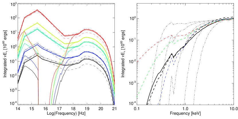
Figure 24.— Left: Integrated intrinsic spectra (thick solid lines) from simulations A1, A2, A3, A4, and A5 (black, blue, green, yellow, red, respectively), with virial velocities $V_{\rm vir}=80,\,113,\,160,\,226,\,{\rm and}\ 320\,{\rm km\,s^{-1}}$. The predicted integrated spectra from our model for quasar lifetimes are shown as dot-dashed lines, and the prediction of a “light bulb” model, where the same total energy is radiated at $L=L_{\rm peak}$, as dashed lines. Integrated observed spectra are shown as thin solid lines. Right: Integrated observed X-ray spectrum from the A3 simulation (thick black line), compared with the integrated intrinsic spectrum, reddened by various column density distributions: our fitted $N_{\rm H}$ distributions from § 2.3 (thick black dashed line), constant (luminosity-independent) lognormal $N_{\rm H}$ distribution with $\bar{N}_{H}=10^{22}\ {\rm cm^{-2}}$ and $\sigma_{N_{H}}=0.4,\,0.7,\,1.0$ (blue, green, and red dashed lines, respectively), and constant $N_{\rm H}=10^{21},\,10^{21.5},\,10^{22},\,10^{22.5},\ {\rm and}\ 10^{23}\ {\rm cm^{-2}}$ (thin dot-dashed lines).

We can test our model by examining whether the quasar luminosity function, relic AGN mass distribution, and X-ray background can be simultaneously reproduced in a self-consistent manner. Because our formulation describes the birthrate of quasars with a peak luminosity $L_{\rm peak}$, it is most useful to consider the integrated energy spectrum of such a quasar over its lifetime,

$$\nu E_{\nu}=\int{{\rm d}t\,\nu L_{\nu}(t)}=\int{\nu f_{\nu}(L)L\,\frac{{\rm d}t(L,L_{\rm peak})}{{\rm d}\log L}\,{\rm d}\log L},$$ (38)

where $f_{\nu}(L)$ is the bolometric correction ($L_{\nu}\equiv f_{\nu}\,L$). As an example, Figure 24 shows the integrated intrinsic spectra (thick solid lines) from the simulations A1, A2, A3, A4, and A5, described in § 2.1. The final black hole masses for these simulations are $M^{f}_{\rm BH}=7\times 10^{6},\,3\times 10^{7},\,3\times 10^{8},\,7\times 10^{8},\,{\rm and}\ 2\times 10^{9}\,M_{\sun}$, respectively. The integrated spectral shape in the X-ray, in particular, is ultimately determined by the observationally motivated bolometric corrections of Marconi et al. (2004), with a reflection component in the X-ray determined following Magdziarz & Zdziarski (1995), and, in the case of the observed spectrum, the distribution of column densities calculated from the simulations. Using our fits to the lifetime ${\rm d}t/{\rm d}\log{L}$ as a function of instantaneous and peak luminosities, we can calculate the expected $\nu E_{\nu}$ from the integral above. These integrated spectra are shown as the dot-dashed lines in the figure, and agree well with the actual integrated spectra of the simulations, demonstrating the self-consistency of our model and applicability of our fitted lifetimes.

This can be compared to idealized models for the quasar lifetime, where we allow the quasar to radiate just at its peak luminosity $L_{\rm peak}\approx L_{\rm Edd}(M^{f}_{\rm BH})$ for some fixed lifetime $t_{Q}^{0}$. We determine $t_{Q}^{0}$ by demanding that the total energetics be correct, $L_{\rm peak}t_{Q}^{0}=\epsilon_{r}M^{f}_{\rm BH}c^{2}$. The predicted integrated energy spectra are shown as the dashed lines, and under-predict the soft and hard X-ray energy output by a factor $\sim 1.5-2$. This is because higher-luminosity quasars tend to have a larger fraction of their energy radiated in the UV-optical rather than the X-ray (e.g., Wilkes et al., 1994; Green et al., 1995; Vignali et al., 2003; Strateva et al., 2005), reflected in our bolometric corrections. Thus, assuming that the quasar spends all its time at $L_{\rm peak}$ does not account for extended times at lower luminosity, where the ratio of X-ray to total luminosity is higher, which would generate an integrated spectrum with a larger fraction of its energy in the X-ray. Assuming that the quasar undergoes pure Eddington-limited growth to its peak luminosity produces an almost identical integrated spectrum to this light-bulb model, as it is similarly dominated by $L\sim L_{\rm peak}$.

Of course, the intrinsic integrated energy spectrum of the simulations is not what determines the X-ray background, but rather the integrated observed spectrum is the critical quantity. This is shown as the thin lines in the left panel of Figure 24, and in detail for our fiducial A3 simulation in the right panel of the figure (thick solid line). Along a given sightline, the observed integrated spectrum will be

$$\nu\frac{{\rm d}E_{\nu}}{{\rm d}\Omega}=\int{{\rm d}t\,\nu\frac{L_{\nu}(t)}{4\pi}\,e^{-\tau_{\nu}(\Omega,\,t)}},$$ (39)

where $\tau_{\nu}$ is the optical depth at a given frequency. We can integrate over solid angle and obtain

$$\nu E_{\nu,\,{\rm obs}}=\int{\nu f_{\nu}\langle e^{-\tau_{\nu}}\rangle\,L\,\frac{{\rm d}t(L,L_{\rm peak})}{{\rm d}\log L}\,{\rm d}\log L},$$ (40)

where $\langle e^{-\tau_{\nu}}\rangle$ is the averaged $e^{-\tau_{\nu}}$ over the column density distribution $P(N_{\rm H}|L,L_{\rm peak})$. Using our fits to the column density distribution and quasar lifetimes and calculating $\nu E_{\nu,\,{\rm obs}}$ as above, we reproduce the integrated observed spectrum quite well (black dashed line). For comparison, we show that it is not a good approximation to redden the spectrum with a constant $N_{\rm H}$, giving the results for $N_{\rm H}=10^{21},10^{21.5},10^{22},10^{22.5},\ {\rm and}\ 10^{23}\ {\rm cm^{-2}}$ (thin dot-dashed lines). Even allowing for a distribution of $N_{\rm H}$ values, the resulting spectrum is a poor match to the observed one if that distribution is taken to be static (i.e. luminosity-independent, as in traditional torus models, for example). We show the results of reddening the intrinsic spectrum by such a (Gaussian) distribution, varying the dispersion $\sigma_{N_{H}}=0.4,\,0.7,\,1.0$ (blue, green, and red dashed lines, respectively), for a median column density $\bar{N}_{H}=10^{22}\ {\rm cm^{-2}}$, the median column density expected around $L_{\rm peak}$ in this simulation. Therefore, the luminosity and host system property dependence of both quasar lifetimes and the column density distribution must be accounted for in attempting to properly predict the X-ray background spectrum from observations of the quasar luminosity function. Finally, note that the hard cutoff in the observed UV spectra at 912Å owes to our calculated cross-sections being incomplete in the extreme UV. Properly modeling the escape fraction and observed emission at these frequencies, while not important for the X-ray background, is critical to calculating the contribution of quasars to reionization, and requires a more detailed modeling of scattering and absorption, especially in the bright optical quasar phase.

7.2. The Integrated X-Ray Background

Given the volume emissivity $j_{\nu}(z)$ (per unit comoving volume) of some isotropic process at a given frequency at redshift $z$, the resulting background specific intensity at frequency $\nu_{0}$ at $z=0$ is (Peacock, 1999)

$$I_{\nu_{0}}=\frac{c}{4\pi}\int{\frac{j_{\nu}[(1+z)\nu_{0},z]}{(1+z)H(z)}}{\rm d}z.$$ (41)

If we were to consider the emissivity $j_{\nu}$ per unit physical volume, there would be an extra factor of $(1+z)^{-3}$ in the integral above. In § 7.1, we determined the integrated observed energy $E_{\nu,\,\rm obs}(L_{\rm peak})$ produced by a quasar with peak luminosity $L_{\rm peak}$. We have also inferred $\dot{n}(L_{\rm peak})(z)$ in § 3.2, the rate at which quasars of peak luminosity $L_{\rm peak}$ are created per unit comoving volume per unit cosmological time. Therefore, the comoving volume emissivity is just

$$j_{\nu}(z)=\int{E_{\nu,\,\rm obs}(L_{\rm peak})\,\dot{n}(L_{\rm peak})\,d\log L_{\rm peak}},$$ (42)

or, expanding $E_{\nu,\,\rm obs}$,

$$j_{\nu}(z) = \int{d\log L_{\rm peak}\int{d\log L}}$$ (43)

$$\times f_{\nu}\langle e^{-\tau_{\nu}}\rangle\,L\,\frac{dt(L,L_{\rm peak})}{{\rm d}\log L}\,\dot{n}(L_{\rm peak}).$$

If the column density distribution were independent of $L_{\rm peak}$, as is assumed in even luminosity-dependent torus models or observationally determined $N_{\rm H}$ functions used for X-ray background synthesis (e.g., Ueda et al., 2003), then we could combine terms in $L_{\rm peak}$ and integrate over them. This simplification, along with the definition of the luminosity function in terms of $L_{\rm peak}$, gives the more traditional formula for the X-ray background in terms of only the observed column density distribution and luminosity function,

$$j_{\nu}(z)=\int{d\log L\,\frac{d\Phi}{d\log L}L_{\nu}\langle e^{-\tau_{\nu}}\rangle}.$$ (44)

However, as we showed in § 3.3 and § 7.1, neglecting the dependence on $L_{\rm peak}$ is not a good approximation at all luminosities and gives an inaccurate estimate of the integrated quasar spectrum; therefore, “purely observation-based” synthesis models of the X-ray background will be inaccurate in a similar manner to synthesis models with an inappropriate model for the quasar lifetime. Essentially, this “averages out” the varying distribution of column densities with $L_{\rm peak}$, which changes the shape of the spectrum in a non-linear manner, especially when integrated over varying bolometric corrections as shown above.

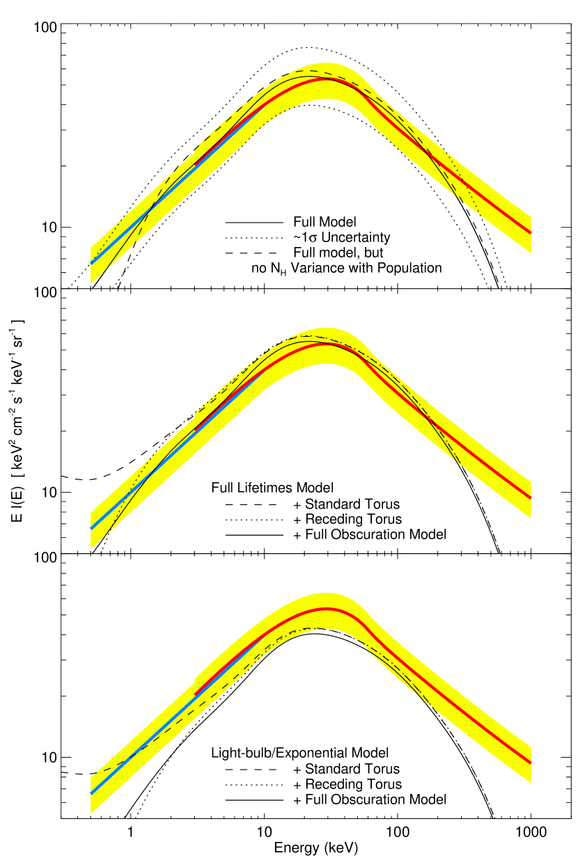
Figure 25.— Predicted integrated X-ray background spectrum (solid black line) from our model of quasar lifetimes and attenuation, with the peak luminosity distribution $\dot{n}(L_{\rm peak})$ determined from the luminosity function. Blue and red thick lines show the observed spectrum from Barcons et al. (2000) and Gruber et al. (1999), respectively. The shaded yellow area illustrates the uncertainty in normalization between both samples (alternatively, $2\sigma$ errors in the Barcons et al. 2000 normalization). The predictions given $1\sigma$ deviations in the fitted $\dot{n}(L_{\rm peak})$ distribution (dotted lines) and given the $\dot{n}(L_{\rm peak})$ distribution determined from hard X-ray data only (dashed line) are shown in the upper panel. Middle panel shows the prediction using our modeling of quasar lifetimes but different models of obscuration, lower panel the prediction with a “light-bulb” or exponential (constant Eddington ratio) model and different obscuration models.

Figure 25 (upper panel) shows the predicted X-ray background spectrum from our full modeling of quasar lifetimes and obscuration (solid lines). We use our analytical fits to the quasar lifetime and column density distributions as in § 7.1 above, as Figure 24 demonstrates that they accurately reproduce the actual integrated quasar X-ray spectra of the simulations, and the analytical forms are integrated over all luminosities and redshifts. The dotted lines show the deviation resulting from shifting the parameters describing our fitted $\dot{n}(L_{\rm peak})$ distribution by $1\sigma$ in either direction, although degeneracies in the parameters suggest that the actual uncertainty in the background prediction is smaller. The dashed line shows the predicted X-ray background if we ignore the broadening of the $N_{\rm H}$ distribution across simulations ($\sigma_{N_{H}}=1.2$) and instead consider only the dispersion of an individual simulation at a given luminosity ($\sigma_{N_{H}}=0.4$).

These can be compared to the observations of Gruber et al. (1999) (red curve, for $E\geq 3\,{\rm keV}$) and Barcons et al. (2000) (cyan curve, for $E\leq 10\,{\rm keV}$). We increase the normalization of the Gruber et al. (1999) spectrum to match that of the best estimate from Barcons et al. (2000) over the range of overlap, determined from combined ASCA, BeppoSAX, and ROSAT data to be $10.0^{+0.6}_{-0.9}\,{\rm keV\,cm^{-2}\,s^{-1}\,sr^{-1}\,keV^{-1}}$ at 1 keV. The uncertainty in the normalization between the two samples, $\sim 20\%$, is shown as the shaded yellow range (alternatively, this represents the $\sim 2\sigma$ errors in the ROSAT normalization).

In the middle panel of the figure, we calculate the predicted X-ray background using our full model of the quasar lifetime, but with different models for quasar obscuration. The solid black line shows the prediction using our full model of quasar obscuration, and is identical to the solid black line in the upper panel. The observations are likewise shown in an identical manner to the upper panel. The dashed black line is the prediction adopting the standard torus model for quasar obscuration, and the dotted line adopts the receding (luminosity-dependent) torus model. These models produce the same overall $\sim 30\,$keV normalization, as this is relatively unaffected by obscuration, but they predict a slightly ($\sim 20\%$) higher background at low energies, giving a slightly softer spectrum. This may appear counterintuitive, given that in Figure 12 these models tend to overpredict the number of high-column density sources, but this is because these models predict a strongly bimodal column density distribution, with unobscured sightlines encountering negligible column densities. These unobscured sightlines dominate the soft X-ray integrated spectrum, where the large column densities through the torus attenuate the quasar spectrum heavily. However, this net offset in the predicted background spectrum is generally within the range of the systematic theoretical and observational uncertainties, and can further be alleviated by tuning the parameters of the torus model to fit the X-ray background spectrum (e.g. Treister & Urry 2005, although their fits require a larger fraction of Compton-thick $N_{\rm H}\sim 10^{25}\,{\rm cm^{-2}}$ sources than shown for even the receding torus model in Figure 12). The feature at $\lesssim 5\,$keV in the standard torus model prediction is a consequence of assuming that “unobscured” lines of sight encounter negligible column density, and does not appear if such sightlines encounter moderate ($\sim 10^{21}\,{\rm cm^{-2}}$) columns.

The lower panel of the figure shows the predicted X-ray background spectrum if we instead consider a light-bulb or exponential light curve (fixed Eddington ratio) model for the quasar lifetime, again with various descriptions of quasar obscuration. In such models, the predicted X-ray background spectrum is independent of the quasar lifetime or characteristic Eddington ratio assumed (see Equation 44). However, as shown in Figure 24, these models do imply a different integrated spectrum for quasars; i.e. different effective bolometric corrections for predicting the X-ray background. In particular, in this model, the observed quasar spectrum at a given luminosity (averaged over the quasar population at that luminosity) is the same as the “effective” quasar spectrum one would use to calculate the total contribution to the X-ray background from quasars of the corresponding observed or peak luminosity, whereas this is not true in our model of quasar lifetimes. The observations are shown in the same manner as the preceding panels. The black solid line shows the prediction with this simplified model for the quasar lifetime, but still adopting our full model for obscuration as a function of instantaneous and peak luminosity, the dashed line assumes instead a standard torus model for obscuration, and the dotted line assumes a receding torus for the obscuration. The variations among different obscuration models are relatively small at most energies, and similar to those discussed above adopting our full model of quasar lifetimes.

In all three cases, however, this model for the quasar lifetime significantly under-predicts the X-ray background, particularly at the $\sim 30\,$keV peak. This shortfall is well-known, and earlier attempts (e.g., Madau et al., 1994; Comastri et al., 1995; Gilli et al., 1999, 2001; Pompilio et al., 2000; Ueda et al., 2003) have generally had to invoke additional assumptions about large obscured populations or a strong increase in the obscured fraction with redshift, neither of which is consistent with observations (e.g., Hasinger, 2002; Barger et al., 2003; Ueda et al., 2003; Szokoly et al., 2004; Barger et al., 2005). The difference between the predictions of various quasar lifetime models is, as explained above, attributable to the difference between the integrated quasar spectrum produced in our full model of the quasar lifetime (in which quasars spend long periods of time at low luminosities, with harder X-ray spectra), and the integrated spectrum in these simplified quasar lifetime models, which is proportional to the instantaneous quasar spectrum, and therefore underpredicts the hard X-ray portion of the spectrum by as much as $\sim 50\%$.

Our prediction of the X-ray background agrees well with the observed spectrum over the range $\sim 1-100\,{\rm keV}$. (At energies above $100\,{\rm keV}$ it is likely that processes we have not included, such as those involving magnetic fields, contribute significantly to the background.) Unlike previous synthesis models for the X-ray background, we are able to do so without invoking assumptions about large Compton thick populations or larger obscured populations at different redshifts. In part, this is because our modeling allows us to predict, based on $\dot{n}(L_{\rm peak})$ and our column density formulation, the population of Compton thick sources (see Figure 12). However, as we have demonstrated, it is primarily because the deficit in previous synthesis models can be attributed to their inability to properly account for the dependence of quasar lifetimes and attenuation on both the instantaneous quasar luminosity and the host system properties (peak luminosity). Our picture, on the other hand, yields an estimate for the X-ray background spectrum that is simultaneously consistent with the observed supermassive black hole mass distribution and total density, as well as the “luminosity-dependent density evolution” observed in X-ray samples (Hopkins et al., 2005f). The background is primarily built up from $z\sim 2.5$ to $z\sim 0.5$, as is evident from the evolution of the black hole mass density in Figure 22, although a harder spectrum at low luminosities will weight this slightly towards lower redshifts (where more low-luminosity quasars are forming). Compton thick and relaxing, low-luminosity sources are accounted for, not as large, independent populations, but as evolutionary phenomena continuously connected to the “normal” quasar population.

8. Discussion

8.1. General Implications of our Model

Our modeling suggests two important paradigm shifts in interpreting quasar populations and evolution:

(1) First, as proposed in Hopkins et al. (2005c), a proper accounting of the luminosity dependence of quasar lifetimes (as opposed to models in which quasars grow in a pure exponential fashion or turn on and off as “light bulbs”) implies a novel interpretation of the luminosity function. The steep bright end (luminosities above the “break” in the luminosity function) consists of quasars radiating near their Eddington limits and is directly related to the distribution of intrinsic peak luminosities (or final black hole masses) as has been assumed previously. However, the shallow, faint end of the luminosity function describes black holes either growing in early stages of activity or in extended, quiescent states going into or coming out of a peak bright quasar phase, with Eddington ratios generally between $l\sim 0.01$ and 1. The “break” luminosity in the luminosity function corresponds directly to the peak in the birthrate of quasars as a function of peak luminosity $\dot{n}(L_{\rm peak})$.

This interpretation resolves inconsistencies in a number of previous theoretical studies. For example, semi-analytical models of the quasar luminosity functions (e.g., Kauffmann & Haehnelt, 2000; Haiman & Menou, 2000; Wyithe & Loeb, 2003) assume, based on simplified models for the quasar lifetime, that quasars at the faint end of the luminosity function correspond to low final-mass black holes (low $L_{\rm peak}\sim L$), presumably in small halos. Consequently, these models overpredict the number of active low-mass black holes (as estimated from radio source counts), especially at high redshift, by orders of magnitude (Haiman, Quataert, & Bower, 2004), and overpredict the number of low-mass spheroids and red galaxies observed (Hopkins et al., 2005e).

Moreover, both observations (McLure & Dunlop, 2004) and comparison of the present-day black hole mass function with radio and X-ray luminosity functions (e.g. Merloni, 2004) suggest anti-hierarchical evolution for the growth of supermassive black holes, where the most massive black holes were produced mainly at high ($z\gtrsim 2$) redshift, and low-mass black holes mostly formed later, which does not follow from idealized descriptions of quasar lifetimes and the luminosity function (for a review, see e.g. Combes 2005).

A one-to-one correspondence between observed luminosity and black hole mass does produce anti-hierarchical behavior in some sense at the high-mass end, because the most massive black holes are formed at $z\sim 2-3$ during the peak of bright quasar activity and the quasar luminosity function evolves to lower luminosities at lower redshifts (as is also the case for our model because the bright end of the luminosity function is dominated by sources near their peak luminosities). However, at black hole masses equal to or below $\sim 10^{8}\,M_{\sun}$ (i.e. galaxies of stellar mass $\lesssim 10^{11}\,M_{\sun}$), the evolution in the quasar luminosity function implies a roughly constant production of black holes with these masses at all redshifts, which is inconsistent with observations of galaxy spheroids indicating that typical ages increase with mass, ruling out a large population of low-mass spheroids with ages equal to or older than those of high-mass spheroids (e.g., Treu et al., 2001; van Dokkum et al., 2001; Treu et al., 2002; van Dokkum & Stanford, 2003; Gebhardt et al., 2003; Rusin et al., 2003; van de Ven et al., 2003; Wuyts et al., 2004; Treu et al., 2005; Holden et al., 2005; van der Wel et al., 2005; di Serego Alighieri et al., 2005; Nelan et al., 2005). As demonstrated in Figure 23, such a model does not produce anti-hierarchical growth or any age gradients within the high-mass spheroid population, also inconsistent with observations. Even given observed “luminosity-dependent density evolution” (e.g. Page et al., 1997; Miyaji et al., 2000, 2001; La Franca et al., 2002; Cowie et al., 2003; Ueda et al., 2003; Fiore et al., 2003; Hunt et al., 2004; Cirasuolo et al., 2005; Hasinger, Miyaji, & Schmidt, 2005), implying that the densities of lower redshift quasars peak at lower redshift, the inferred anti-hierarchical evolution if observed luminosity directly corresponds to black hole mass (i.e. as in “light-bulb” or “fixed Eddington ratio” models) is not strong enough to account for observed anti-hierarchical growth of the corresponding galaxy spheroids (Hopkins et al., 2005e).

Furthermore, in these earlier models, a “break” in the luminosity function is not necessarily reproduced (Wyithe & Loeb, 2003), and the faint-end slope has no direct physical motivation. The break may be caused by feedback mechanisms which set a characteristic turnover in both the galaxy mass function and quasar luminosity function (e.g., Scannapieco & Oh 2004; Dekel & Birnboim 2004), as in our modeling. The $\dot{n}(L_{\rm peak})$ distributions in our model and “light bulb” or “fixed Eddington ratio” models are comparable at and above the break in the quasar luminosity function, and therefore make similar predictions for some observations at these luminosities. However, the faint-end slope has a different physical motivation in our model. Unlike the bright-end slope, which is determined directly by the active final black hole mass function or peak luminosity distribution (in essentially all models of the quasar lifetime), the faint-end slope in our modeling is a consequence of the quasar lifetime as a function of luminosity, and is a prediction of our simulations and modeling almost independent of the underlying faint-end slope of the active black hole mass function or peak luminosity distribution. In Hopkins et al. (2005f) we examine this in more detail, and demonstrate that it predicts well the evolution in the faint-end quasar luminosity function slope with redshift and the observed “luminosity-dependent density evolution” in many samples (Page et al., 1997; Miyaji et al., 2000, 2001; La Franca et al., 2002; Cowie et al., 2003; Ueda et al., 2003; Fiore et al., 2003; Hunt et al., 2004; Cirasuolo et al., 2005; Hasinger, Miyaji, & Schmidt, 2005).

Other observational evidence for our picture exists; for example in the observed distribution of Eddington ratios (see § 5), the distribution of low-redshift, active black hole masses (see § 4.3), and the turnover in the expected distribution of black hole masses in early-type galaxies at $\sim 10^{8}\,M_{\sun}$ (e.g., Sheth et al., 2003). Total (integrated) quasar lifetimes estimated from observations are inferred to increase with increasing black hole mass as we predict (Yu & Tremaine, 2002), and furthermore, the Eddington ratios of observed quasar samples are seen to increase systematically with redshift, as the sample becomes increasingly dominated by luminosities above the break in the luminosity function (McLure & Dunlop, 2004).

Moreover, observations show that the evolution of the luminosity function with decreasing redshift is driven by a decrease in the characteristic mass scale of actively accreting black holes (e.g., Heckman et al., 2004), which can be explained in our model by the relation of the observed luminosity function to the peak in the distribution of active black hole masses $\dot{n}(L_{\rm peak})$. This observation, however, has caused considerable confusion, as observations of both radio-quiet (Woo & Urry, 2002) and radio-loud (O’Dowd et al., 2002) local (low redshift) AGN indicate that nuclear and host luminosities are uncorrelated, implying that nuclear luminosity does not depend on black hole mass (Heckman et al., 2004), and therefore that the primary variable determining the nuclear luminosity is the Eddington ratio, with the luminosity function spanning a broad range in Eddington ratios (Hao et al., 2005). Furthermore, observations show that this is not true of high redshift quasars, as both direct estimates of accretion rates (e.g., Vestergaard, 2004; McLure & Dunlop, 2004) and the fact that their high luminosities would yield unreasonably large black hole masses rule out substantially sub-Eddington accretion rates for most objects. Many previous empirical and semi-analytical models could not simultaneously account for these observations. To explain just the low-redshift observations, such models adopt tunable distributions of Eddington ratios fitted to the data. However, both these observations are consequences of our interpretation of the luminosity function, as observations of local AGN and the low-redshift luminosity function are dominated by quasars below the break in the luminosity function, which are undergoing sub-Eddington growth and span a wide range of Eddington ratios, while observations at high redshift are dominated by bright objects at or above the break in the luminosity function, which are undergoing Eddington-limited (or near Eddington-limited) growth near their peak luminosity (see § 5).

(2) The second paradigm shift indicated by our modeling is that quasar obscuration is not a static or quasi-static geometric effect, but is primarily an evolutionary effect. The physical reasoning for this is simple: the massive gas inflows required to fuel quasar activity produce large obscuring columns, and so column densities are correlated with quasar luminosity. The basic picture of buried quasar activity associated with the early growth of supermassive black holes and starburst activity has been proposed previously and studied for some time (e.g., Sanders & Mirabel, 1996; Fabian, 1999), but our modeling allows us to describe the evolution of obscuration in a self-consistent manner, defining obscured and unobscured phases appropriately and identifying dynamical correlations between the column density distribution and instantaneous and peak luminosities.

There is substantial observational support for this picture. Point-like X-ray sources have been observed in many bright sub-millimeter or infrared and starburst sources, with essentially all very luminous infrared galaxies showing evidence of buried quasar activity (e.g., Sanders & Mirabel, 1996; Komossa et al., 2003; Ptak et al., 2003), indicating simultaneous buried black hole growth and star formation at redshifts corresponding to peak quasar activity ($z\gtrsim 1$) (Alexander et al., 2005a, b). The buried black holes in high-z starbursting galaxies appear to be active but undermassive compared to the quiescent galaxy black hole-stellar mass relation (Borys et al., 2005), implying that they are rapidly growing in the starburst but have not yet reached their final masses, presumably set in the subsequent “blowout” phase. Similarly, observations suggest that obscured AGN are significantly more likely to exhibit strong sub-millimeter emission characteristic of star formation, implying both that obscured black hole growth and star formation are correlated and that obscuration mechanisms (responsible for re-radiation in the submm and IR) may be primarily isotropic in at least some cases (e.g., Page et al., 2004; Stevens et al., 2005). Evidence from quasar emission line structure (e.g., Kuraszkiewicz et al., 2000; Tran, 2003), directly related to the inner broad-line region, suggests that isotropic obscuration of quasars can be important, in contradiction to angle-dependent models. Finally, many observations (e.g., Steffen et al., 2003; Ueda et al., 2003; Hasinger, 2004; Grimes, Rawlings, & Willott, 2004; Sazonov & Revnivtsev, 2004; Barger et al., 2005; Simpson, 2005) indicate that the fraction of broad-line or obscured quasars is a function of luminosity, which cannot be accounted for in traditional static “torus” models (e.g., Antonucci, 1993) or reproduced even by modified luminosity-dependent torus models (Lawrence, 1991), an observation that is explained by our model (see § 4 for a detailed discussion).

Much of the obscuration in our modeling comes from large scales, arising from the inner regions of the host galaxy on scales $\sim 50\,$pc or larger. While our resolution limits prevent our ruling out the possibility of gas collapse to a dense, $\sim\,$pc scale torus surrounding the black hole, during the peak obscured phases of the final merger, our simulations indicate that these large scales dominate the contribution to the column density, with quite large columns, which should be observationally testable. Indeed, this is suggested by the typical scales of obscuration in starbursting systems (e.g. Soifer et al. 1984a,b; Sanders et al. 1986, 1988a,b; for a review, see e.g. Soifer et al. 1987), given that, as discussed above, the dominant obscured phase of growth is closely associated with a starburst as implied observationally (Alexander et al., 2005a, b; Borys et al., 2005).

Observations of polarized light in intrinsically bright Type II AGN with unobscured luminosities typical of quasars (as opposed to local, dim Seyfert II objects in relaxed hosts) show scattering on large scales $\sim$kpc, and in some cases obscuration clearly generated over scales extending beyond the host galaxy in the form of distortions, tidal tails, and streams from interactions and major mergers (Zakamska et al., 2004, 2005). The angular structure seen in these observations is consistent with our modeling. Moreover, in optically faint X-ray quasars (e.g. Donley et al., 2005) it appears that obscuration is generated by the host galaxies, and is directly related to host galaxy morphologies and line-of-sight distance through the host. The critical point is that, regardless of the angular structure of obscuration, typical column densities are strongly evolving functions of time, luminosity, and host system properties, and the observed distribution of column densities is dominated by these effects, not by differences in viewing angle across a uniform population. This is the case in our modeling as the lognormal dispersion (across different lines of sight) in column densities is $\sigma_{N_{H}}\sim 0.4$ for a given simulation at some instant, whereas typical column densities across simulations, as a function of instantaneous and peak luminosities, span several orders of magnitude from $N_{\rm H}\sim 10^{18}-10^{26}\ {\rm cm^{-2}}$.

8.2. Specific Predictions of our Model

Our predictions include:

• Quasar Lifetimes: We find that for a particular source, the quasar lifetime depends sensitively on luminosity, with the observed lifetime in addition depending on the observed waveband. Intrinsic quasar lifetimes vary from $t_{Q}\sim 10^{6}-10^{8}$ yrs, with observable lifetimes $\sim 10^{7}$ yrs in optical B-band (Hopkins et al., 2005a, b), in good agreement with observational estimates (for a review, see Martini, 2004).

• Luminosity Functions: Using a parameterization of the intrinsic distribution of peak luminosities (final quasar black hole masses) at a given redshift, our model of quasar lifetimes allows us to reproduce the observed luminosity function at all luminosities and redshifts $z=0-6$. Although this is an empirical determination of the peak luminosity distribution, it implies a new interpretation of the luminosity function (Hopkins et al., 2005c), which provides a physical basis for the observed “break” corresponding to the peak in the peak luminosity distribution. Moreover, the faint end slope is not determined by our empirical fitting procedure, but instead by the dependence of the quasar lifetime on luminosity, with its value and redshift evolution predicted by our modeling (Hopkins et al., 2005f). The evolution of typical column densities in different stages of merger activity produces a significant population of obscured quasars, accounting for the difference between hard X-ray (e.g., Ueda et al., 2003), soft X-ray (e.g., Miyaji et al., 2001), and optical B-band (e.g., Croom et al., 2004) luminosity functions (§ 3.2).

• Column Density Distributions: The evolution of the column densities in our simulations reproduces the observed distribution of columns in optically-selected quasar samples, when the appropriate selection criteria are applied (Hopkins et al., 2005b), as well as complete column distributions in hard X-ray selected samples (§ 3.3). Column density evolution over the course of a merger yields a wider observed distribution of columns than that produced across different viewing angles at a given point in a merger.

• Broad Line Luminosity Function and Fraction: Using our simulations to estimate when quasars will be observable as broad-line objects (either based on the ratio of quasar to host galaxy optical B-band luminosity or the obscuring column density), we reproduce the luminosity function of broad-line quasars in hard X-ray selected samples as well as optical broad-line quasar surveys, and the fraction of broad-line quasars in a given sample as a function of luminosity, to better precision than traditional or luminosity-dependent (but non-dynamical) torus models which are fitted to the data (§ 4.2). By providing an a priori prediction of the broad-line fraction as a function of luminosity and redshift which depends systematically on the typical quasar host galaxy gas fraction, we propose that observations of the broad line fraction at different redshifts can be used to constrain the gas fraction of quasar hosts and its evolution with redshift.

• Active Black Hole Mass Functions: Using our prescription for deciding when objects will be visible as “broad-line” quasars, we predict the distribution of low-redshift, broad-line and non-broad line active quasar masses, in good agreement with observations from the SDSS, with expected incompleteness in the observed sample at low $M_{\rm BH}\lesssim 10^{6}\,M_{\sun}$ black hole masses (§ 4.3). This is a new prediction which can be tested in greater detail by future observations, and our calculations allow us to model the differences in active black hole mass functions of the Type I and Type II populations. The width of the expected broad-line black hole mass function depends significantly on the model of quasar lifetimes, enabling such measurements to probe the statistics of quasar evolution.

• Eddington Ratios: We determine Eddington ratio distributions from our simulations, given the peak luminosity distribution implied by the observed quasar luminosity function. The predicted distribution, once the appropriate observed magnitude limit is imposed, agrees well with observations at both low ($z<0.5$) and high ($1.5<z<3.5$) redshifts (§ 5). As noted above, our interpretation of the luminosity function explains seemingly contradictory observations of Eddington ratios at different redshifts. There is even a suggestion (Cao & Xu, 2005) that the evolution of quasars seen in our simulations (with bright phases in mergers and extended relaxation after) can account for observations of bimodal Eddington ratio distributions at $z\sim 0$ (Marchesini et al., 2004), when coupled with an appropriate description of radiatively inefficient accretion phases, although it is possible that many of these low-redshift black holes are not fueled by mergers, especially in e.g. low-luminosity Seyferts.

• Relic Black Hole Mass Function: With our model for quasar lifetimes, the luminosity function at a given redshift implies a birthrate of sources with given peak luminosities, $\dot{n}(L_{\rm peak})$, which translates to a distribution in final black hole masses. Integrating this over redshift, we predict the present-day mass distribution and total mass density of supermassive black holes. They agree well with observational estimates inferred from local populations of galaxy spheroids. In our picture, these spheroids are produced simultaneously with the supermassive black holes they harbor (§ 6). We demonstrate that the integrated supermassive black hole density, quasar flux density, and number counts in different wavebands can be reconciled with a radiative efficiency $\epsilon_{r}=0.1$, satisfying the constraints of counting arguments such as that of Soltan (1982). Further, we show in § 2.4 and § 4.1 that the corrections to such observational arguments based on optical quasar samples are small (order unity) when we account for the luminosity dependence of quasar lifetimes, despite an extended obscured phase of quasar growth. In other words, although a quasar spends more time obscured than it does as a bright optical source, the total mass growth and radiated energy are dominated by the final “blowout” stage visible as a bright optical quasar.

• X-ray Background: The integrated quasar spectrum from our models of quasar lifetimes and column densities as a function of instantaneous and peak luminosities can be combined with the birthrate of quasars with a given peak luminosity to give the integrated cosmic background in any frequency range. We predict both the normalization and shape of the X-ray background from $\sim 1-100$ keV, with our modeling accounting for quasar obscuration as an evolutionary process (with a corresponding population of Compton-thick objects), avoiding any need for arbitrary assumptions about additional obscured populations (§ 7.2). For any model in which the quasar spectrum depends on luminosity or accretion rate, we demonstrate that a proper modeling of the quasar lifetime is critical to reproducing observed backgrounds.

• Correlation Functions: In Lidz et al. (2005), we predict the quasar correlation function and bias as a function of redshift and luminosity using our model, and compare it to that expected using “light bulb” or exponential light curves. As most quasars in our modeling have a characteristic peak luminosity or final black hole mass corresponding to the peak of the $\dot{n}(L_{\rm peak})$ distribution, they reside in hosts of similar mass, and there is little change in bias with luminosity at a given redshift, in contrast to idealized models for the quasar lifetime and luminosity function. Our predicted bias agrees well with the observations of Croom et al. (2005), who also find no evidence for a dependence of the correlation on quasar luminosity at a given redshift, as we expect. In fact, Porciani, Magliocchetti, & Norberg (2004) and Croom et al. (2005) find that their observations can be explained if quasars lie in hosts with a constant characteristic mass $\sim 2\times 10^{12}\,M_{\sun}$ ($h=0.7$). If we consider their redshift range $z\sim 1-2$, we predict the quasar population will be dominated by sources with $L_{\rm peak}=L_{\ast}(z)$, which given $M^{f}_{\rm BH}(L_{\rm peak})$ and using the $M_{\rm BH}-M_{\rm halo}$ relation of Wyithe & Loeb (2003) yields a nearly constant characteristic host halo mass $\sim 1-2\times 10^{12}\,M_{\sun}$, in good agreement. Similarly, Adelberger & Steidel (2005) find that the quasar-galaxy cross-correlation function does not vary with luminosity, implying with $\sim 90\%$ confidence that faint and bright quasars reside in halos with similar masses and that fainter AGN are longer lived, strongly disfavoring traditional “light bulb” and exponential light curve models. Furthermore, Hennawi et al. (2005) find an order of magnitude excess in quasar clustering at small scales $\lesssim 40\,h^{-1}\,{\rm kpc}$, with the correlation function becoming progressively steeper at sub-Mpc scales, suggesting that quasar activity is triggered by interactions and mergers.

• Host Galaxy Properties: Because black hole growth and spheroid formation occur together in our picture, our modeling allows us to describe relationships between black hole and galaxy properties. For example, we reproduce both the observed $M_{\rm BH}-\sigma$ relation (Di Matteo et al., 2005; Robertson et al., 2005b) and the fundamental plane of elliptical galaxies (Robertson et al., in preparation). Since we also reproduce the distribution of relic black holes inferred from the $z=0$ distribution of spheroid velocity dispersions or luminosity functions using the observed versions of these relations, our match to these relations indicates that we also reproduce these distributions of host spheroid properties. We consider this in detail in Hopkins et al. (2005e), and find that we are able to account for a wide range of host galaxy properties, including luminosity and mass functions, color-magnitude relations, mass-to-light ratios, and ages as a function of size, mass, and redshift. With our modeling of the quasar lifetime as motivated by our simulations, the evolution and distribution of properties of red-sequence galaxies and the quasar population are shown to be self-consistent, which is not the case for idealized models of quasar evolution.

Aside from an empirical estimate of the distribution of peak quasar luminosities $\dot{n}(L_{\rm peak})$, we determine all of the quantities summarized above self-consistently from the input physics of our simulations, including a physically motivated dynamic accretion and feedback model in which black holes accrete at the Bondi rate determined from the surrounding gas, and $\sim 5\%$ of the radiant energy couples thermally to that gas. Beyond this, our simulations enable us to calculate the various predictions above a priori, without the need for additional assumptions or tunable parameters.

We compare each of these predictions to those obtained using idealized descriptions of the quasar lifetime, i.e. “light-bulb” and exponential light curve (constant Eddington ratio) models, and the column density distribution, i.e. standard and “receding” (luminosity-dependent) torus models. We fit all these (along with our full model) to the observed luminosity function in the same manner (allowing the same degree of freedom to ensure that they all yield the same observed luminosity function), and we fit the free parameters of these tunable models (e.g. typical Eddington ratios and quasar lifetimes for the “light-bulb” or exponential models, typical column densities and torus scalings for the torus models) independently to each observation to maximize their ability to reproduce observations. However, we still find better agreement between our model (with no parameters tuned to match observations) and the observations in nearly every case where the tunable phenomenological model is not guaranteed to reproduce the observation by construction. The one exception is the relic supermassive black hole mass function, for which the predictions of our modeling and idealized lifetime models are essentially identical, reflecting the fact that in both cases black hole growth is dominated by bright, optically observable, high Eddington ratio phases.

Moreover, the best-fit parameters for the idealized models, when fitted independently to each observation, are not self-consistent. For example, calculations of the black hole mass function imply high Eddington ratios $l\sim 0.5-1$ (e.g., Yu & Tremaine, 2002), and our fit to the active black hole mass function (Heckman et al., 2004) suggests $l\sim 1$, but the observed distribution of accretion shows a typical $l\sim 0.3$ (Vestergaard, 2004), and fitting to the broad-line fraction as a function of luminosity with our full obscuration model but these lifetime models implies a lower $l\sim 0.05$. Likewise, fitting torus models to the X-ray background suggests typical column densities through the torus of $N_{\rm H}\sim 10^{25}\,{\rm cm^{-2}}$ (e.g., Treister & Urry, 2005), while fitting to the observed column density distributions (Treister et al., 2004; Mainieri et al., 2005) suggests equatorial columns $N_{\rm H}\lesssim 10^{24}\,{\rm cm^{-2}}$. Clearly then, reproducing the observations listed above, and in particular doing so self-consistently, is not implicit in any model which successfully reproduces the quasar luminosity function, even at multiple frequencies.

8.3. Further Testable Predictions of our Model

Our model for quasar evolution makes a number of observationally testable predictions:

• Quasar lifetimes are only weakly constrained by observations (e.g. Martini, 2004), but future studies may be able to measure both the lifetime of individual quasars and the statistical lifetimes of quasar populations as a function of luminosity. We describe in detail our predictions for the evolution of individual quasars and quantify their lifetimes in § 2, and further predict the distribution of both integrated and differential lifetimes in an observed sample as a function of luminosity. This should provide a basis for comparison with a wide range of observations, with the most important prediction being that the quasar lifetime should increase with decreasing luminosity.

• For a reasonably complete, optically selected sample above some luminosity, the distribution of observed column densities should broaden to both larger and smaller $N_{\rm H}$ values as the minimum observed luminosity is decreased, as both intrinsically faint periods with low column density and intrinsically bright periods with high column density become observable.

• Similarly, the Eddington ratio distribution should be a function of observed luminosity, with a broad distribution of Eddington ratios down to $l\sim 0.01-0.1$ at luminosities well below the break in the observed luminosity function, and a more strongly peaked distribution about $l\sim 0.2-1$ for luminosities above the break (Figure 20).

• In our interpretation, the bright and faint ends of the luminosity function correspond statistically to similar mixes of galaxies, but in various stages of evolution; whereas in all other competing scenarios, the quasar luminosity is directly related to the mass of the host galaxy. Therefore, any observational probe that differentiates quasars based on their host galaxy properties such as, for example, the dependence of the clustering of quasars on luminosity, or the host stellar mass and size as a function of luminosity (although we caution that this is somewhat dependent of the modeling of star formation in mergers), can be used to discriminate our picture from older models. We present a detailed prediction of the quasar correlation function based on our modeling for comparison with observations in Lidz et al. (2005).

• Our distribution $\dot{n}(L_{\rm peak})$ directly translates to a black hole merger rate, as a function of mass, in our modeling, allowing a detailed prediction of the gravitational wave signal from black hole mergers as a function of redshift.

• The broad line fraction as a function of luminosity, defined by requiring that “broad-line” objects have an observed B-band luminosity above a fraction $f_{\rm BL}$ of that of their host galaxy, is a prediction of our model quasar and galaxy light curves. However, the uncertainties are large, primarily because different observational samples have varying sensitivity to quasar vs. host galaxy optical light. Furthermore, the host galaxy gas fraction and $f_{\rm BL}$ are degenerate in these predictions – a well-defined observational sample complete to some $f_{\rm BL}$ can constrain our modeling of quasar fueling and the relation between quasar and host galaxy light curves. In particular, such observations, either by measuring the faint-end shape of the “broad-line” quasar luminosity function or the mean “broad-line” fraction at a given luminosity as a function of redshift, can constrain the gas fractions of quasar host galaxies and their evolution, essentially a free parameter in our empirical modeling.

• We also predict the distribution of active, low-redshift black hole masses in § 4. These predictions can be compared to mass functions for active black holes from numerous quasar surveys, which should include improved mass functions of the entire quasar population complete to lower luminosities as well as future mass functions for the population of active broad-line AGN. We provide predictions for the black hole mass function of all active quasars, and for just the “broad-line” population (as a function of the survey selection).

• Because the evolution of spheroids and supermassive black holes is linked in our modeling, with each affecting the evolution of the other, we can also use the distribution of observed quasar properties to predict galaxy properties such as number counts, spheroid masses and luminosities, and colors as a function of redshift. For the calculation and discussion of these predictions, see Hopkins et al. (2005e).

• In our model, the growth of supermassive black holes is dominated by galaxy mergers. Therefore, at any given redshift, the mass (and as a consequence, luminosity) function of galaxy mergers should have a similar shape to our distribution of quasar birthrates, $\dot{n}(L_{\rm peak})$, distinct from the shapes of either the quasar or total galaxy luminosity functions. Indeed, preliminary observational estimates of both the merger luminosity function (e.g., Xu et al., 2004; Conselice et al., 2003; Wolf et al., 2005) and quasar host galaxy luminosity function (Bahcall et al., 1997; Hamilton et al., 2002), primarily at low redshifts, appear be consistent with this expectation. Theoretically, it may be possible to predict the merger luminosity function using either cosmological simulations or semi-analytical models; we discuss this further in § 9.

8.4. Mock Quasar Catalogs

In principle, our modeling can be used to predict the distributions of quasar luminosities in various wavebands, column densities, active black hole masses, and peak luminosities for a wide range of observational samples, but it is impractical for us to plot predictions of these quantities for all possible sample selection criteria. To enable comparison with a wider range of observations, we have used our modeling and the conditional probability distributions for these quantities from our simulations to generate Monte Carlo realizations of quasar populations, which we provide publicly via ftp.

At a particular redshift, we use our fitted $\dot{n}(L_{\rm peak})$ distribution and our suite of simulations to generate a random population of mock “quasars.” We first generate the peak luminosities of each “quasar” according to the fitted $\dot{n}(L_{\rm peak})$ at that redshift. For each object, we then use the probability of being at a given instantaneous luminosity in simulations with a similar peak luminosity to generate a current bolometric luminosity. In practice, we calculate the $P(L\,|L_{\rm peak})$ distribution by summing $w(L_{\rm peak},\ L_{\rm peak,\ i})\times P(L\,|L_{\rm peak,\ i})$, where $L_{\rm peak}$ is the mock quasar peak luminosity, $L_{\rm peak,\ i}$ is the peak luminosity of each simulation and $w(L_{\rm peak},\ L_{\rm peak,\ i})$ is a Gaussian weighting factor ($\propto\exp(-\log^{2}(L_{\rm peak}/L_{\rm peak,\ i})/2(0.05)^{2})$). Knowing the instantaneous bolometric luminosity $L$ and peak luminosity $L_{\rm peak}$, we then follow an identical procedure to determine the joint distribution $P(X\,|\,L,\,L_{\rm peak})$ of each subsequent quantity $X$, from simulations with similar $L$ and $L_{\rm peak}$. We have compared this with Monte Carlo realizations based on our fitted probability distributions in this paper, and find that essentially identical results are achieved for e.g. the distribution of $L$ and $L_{\rm peak}$, and column densities in phases of growth not near peak luminosity. However, this modeling is not identical for e.g. the distribution of Eddington ratios and column densities around $L\sim L_{\rm peak}$, which reflects the fact that our fits to the Eddington ratio distribution (§ 5) are rough and that our fits to the column density distribution do not apply to the final “blowout” phase of quasar evolution (as discussed in detail in § 4).

For each mock quasar, we generate a peak luminosity, final (post-merger) black hole mass, instantaneous bolometric luminosity, intrinsic (un-attenuated) B-band ($\nu L_{\nu}$ at $\nu=4400$Å), soft X-ray (0.5-2 keV), and hard X-ray (2-10 keV) luminosity, observed (attenuated using the generated column density and the reddening/dust extinction modeling described in § 2.2, with SMC-like reddening curves and extinction following e.g. Pei 1992, Morrison & McCammon 1983) B-band, soft X-ray, and hard X-ray luminosities, column density of neutral hydrogen, column density of neutral+ionized hydrogen, and instantaneous black hole mass. The intrinsic luminosities in each band are calculated using the bolometric corrections described in Marconi et al. (2004), which account for the luminosity dependence of the optical-to-X-ray luminosity ratio $\alpha_{\rm OX}$ (as discussed in § 3.2), and then attenuated to give the observed luminosities. We also provide intrinsic and attenuated luminosities in each waveband using the constant bolometric corrections of Elvis et al. (1994), but we caution that these are not calculated in a completely self-consistent manner, as our assumed bolometric luminosity function to which we fit the $\dot{n}(L_{\rm peak})$ distribution is based on using the luminosity-dependent bolometric corrections. We do not directly calculate Eddington ratios, as these are defined differently in many observed samples, but they should be calculable with the given luminosities and black hole masses.

We calculate these quantities for a mock sample of $\sim 10^{9}$ quasars at each redshift $z=0.2,\ 0.5,\ 1,\ 2,\ {\rm and}\ 3$. Most of these quasars are at luminosities orders of magnitude below those observed, therefore for space considerations and because our predictions become uncertain at low luminosities, we retain only the $10^{6}$ quasars with brightest bolometric luminosities at each redshift. This introduces some uncertainty in our statistics at the lowest luminosities in any given band, but these luminosities are generally still well below those observed in most samples. At any luminosity, but especially at the brightest luminosities, there is also a significant amount of effective “noise” owing to our incomplete sampling of the enormous parameter space of possible mergers, and decreasing total time across simulations spent at large luminosities, which can be estimated from e.g. Figures 8 and 17. Finally, at each redshift, we generate two distributions, reflecting the $\sim 1\sigma$ range in $\dot{n}(L_{\rm peak})$, and roughly parameterizing the degeneracies in our fit to the observed luminosity functions and uncertainty in the faint-end of $\dot{n}(L_{\rm peak})$ – “Fit 1” has a lower $L_{\ast}$ (lower peak in $\dot{n}(L_{\rm peak})$), with a larger $\sigma_{\ast}$ (broader $\dot{n}(L_{\rm peak})$ distribution), and “Fit 2” has a higher $L_{\ast}$ and smaller $\sigma_{\ast}$ (more narrowly peaked $\dot{n}(L_{\rm peak})$ distribution). We show a few example “quasars” from our $z=0.2$ mock distribution in Table 1, to demonstrate the format and units used.

8.5. Starburst Galaxies

Although we do not yet model the re-radiation of absorbed light by dust or the contribution of stellar light to quasar host IR luminosities, including these in our picture for quasar evolution will enable us to predict luminosity functions in the IR and sub-mm and their evolution with redshift. We can at this point, however, estimate if our model for quasar lifetimes and merger-driven evolution with $\dot{n}(L_{\rm peak})$ is consistent with the observed distribution of ultraluminous infrared galaxies. Naively, we might expect that since the obscured quasar phase has a duration up to $\sim 10$ times that of the optically observable quasar phase, there should be $\sim 10$ times as many ULIRGs as bright optical QSOs. But, this neglects the complicated, luminosity dependent nature of quasar lifetimes.

Given that the bright quasars we simulate attain, during their peak growth phase, an intrinsic luminosity comparable to that of the host starburst, and that this period of peak growth has a similar duration to the starburst phase (see Figure 13 and Di Matteo et al., 2005; Springel et al., 2005b), we can estimate (roughly) the ULIRG bolometric luminosity function from our bolometric quasar luminosity function. Thus, the more accurate comparison to the ULIRG luminosity function is with the hard X-ray quasar luminosity function, as this recovers (and at some luminosities can be dominated by) “buried” quasars in starburst phases. This is only applicable above the break in the luminosity function, where quasars are undergoing peak quasar growth. Below the break, quasars are, on average, sub-Eddington and can have luminosities well below that of their star-forming hosts (see Figure 13), so we expect our quasar luminosity function to be significantly shallower than the ULIRG luminosity function at these luminosities. Note also that this does not imply that ULIRGs are all AGN-dominated, as the starburst and peak AGN activity can be (and generally are) somewhat offset, but only says that the lifetime curves at the bright end should be similar.

Considering the luminosity function at $z=0.15$, then, we expect ULIRG densities $d\Phi/{\rm d}M_{\rm bol}\sim 3\times 10^{-7}\ {\rm and}\ 9\times 10^{-8}\ {\rm Mpc^{-3}\,mag^{-1}}$ at $L\sim 1.6\times 10^{12}\,L_{\sun}$ and $2.5\times 10^{12}\,L_{\sun}$, respectively. These estimates are consistent with the observed density in the IRAS 1 Jy Survey (Kim & Sanders, 1998) at a mean redshift $z=0.15$, with ${\rm d}\Phi/{\rm d}M_{\rm bol}\sim 5\times 10^{-7},\ 7\times 10^{-8}\ {\rm Mpc^{-3}\,mag^{-1}}$ (rescaled to our cosmology), and as expected, our quasar luminosity function slope becomes significantly shallower than the observed 1 Jy survey luminosity function slope below $L\sim 10^{11}-10^{12}\,L_{\sun}$, roughly the break luminosity of the luminosity function. We predict these densities to change with redshift according to the evolution of $\dot{n}(L_{\rm peak})$, decreasing by a factor $\sim 1.5$ at $z=0.04$, in good agreement with the evolution of IRAS ULIRG luminosity functions (Kim & Sanders, 1998). Likewise, at $z\sim 1-3$, we predict a mean space density $\Phi(L>10^{11}\,L_{\sun})\sim 1-3\times 10^{5}\ {\rm Mpc^{-3}}$, in agreement with the $\sim 5\times 10^{5}\ {\rm Mpc^{-3}}$ density of such sources expected to reproduce the observed cumulative source density $4\times 10^{4}\,{\rm deg^{-2}}$ of 1 mJy $850\,\mu{\rm m}$ SCUBA sources (Barger et al., 1999). Furthermore, our prediction of the fraction of buried AGN and its evolution with redshift agrees well with determinations from X-ray samples (Barger et al., 2005) and recent Spitzer results in the mid and near-infrared at $z\sim 2$ (Martinez-Sansigre et al., 2005).

8.6. AGN not Triggered by Mergers

Some low redshift quasars (e.g. Bahcall et al. 1996) and many nearby, low-luminosity Seyferts appear to reside in ordinary, relatively undisturbed galaxies. Our picture for quasar evolution does not immediately account for these objects because we suppose that nuclear activity is mainly triggered by tidal torques during a merger.

This work is primarily concerned with the origin of the majority of the mass in spheroids and supermassive black holes, and as a consequence, the relation of this to the abundance and evolution of quasars and the cosmic X-ray background. Based on our present analysis, we believe that a merger-driven picture can account for the main part of each of these, and, as described earlier, that the most relevant phase in the history of the Universe to these phenomena appears to have been at moderate redshifts, $z\sim 2.5$ to $z\sim 0.5$.

Our model does not exclude other mechanisms for triggering AGN and it is likely that a variety of stochastic or continuous processes are relevant to nuclear activity in undisturbed disks and residual low-level accretion in relaxed systems. This is not contrary to our picture because most of the total black hole mass density in the Universe is in spheroid-dominated systems. The principal requirement of our model is that AGN activity in undisturbed galaxies should not contribute a large fraction of the black hole mass density in the Universe, to avoid spoiling tight correlations between the black hole and host galaxy properties and producing too large a present-day black hole mass density in violation of the Soltan (1982) constraint.

For example, if a molecular cloud passed through the center of our Galaxy near Sgr A^∗, it is possible that the Milky Way would resemble a Seyfert for some period of time. Alternatively, it has long been recognized that mass loss from normal stellar evolution of bulge stars or stellar clusters near the centers of galaxies can provide a continuous supply of fuel for low-level accretion (e.g., McMillan et al., 1981; MacDonald & Bailey, 1981; Shull, 1983). Typical galactic stellar mass loss rates ($\dot{M}\sim 1\,M_{\sun}\,{\rm yr^{-1}}\,(10^{11}\,M_{\sun})^{-1}$) yield Bondi-Hoyle accretion rates $\sim 10^{-5}-10^{-4}$ of Eddington in relaxed, dynamically hot systems; and mass loss rates from O and W-R stars ($\dot{M}\sim 10^{-6}\,M_{\sun}\,{\rm yr^{-1}}\,(10\,M_{\sun})^{-1}$) in young, dense star clusters near the centers of galaxies with sufficient cold gas for continued star formation can yield rates as high as $\sim 10^{-2}$ of Eddington.

Even though these fueling mechanisms do not involve mergers, the scenario we have discussed might still be relevant to the origin of these black holes. Of course, the black holes and spheroids in disk-dominated systems may have produced in a manner that did not involve mergers. Alternatively, most of the black hole mass in these objects (which is small compared to that in spheroid-dominated galaxies) could have been assembled long ago in mergers with bright quasar phases and then these “dead” quasars are resurrected sporadically by other fueling mechanisms.

Independent of how these black holes were formed, elements of our modeling may still account for certain observed properties of Seyferts. The observed Seyfert luminosity function appears to join smoothly onto the quasar luminosity function (Hao et al., 2005). It is not obvious that this would be the case if the two types of objects are produced by entirely distinct mechanisms. In addressing this, it is useful to separate the process by which gas is delivered to the black hole from the subsequent evolution that determines the observed activity. In our picture, gas is delivered to the black hole by gravitational torques during a merger, but other mechanisms, like bar-induced fueling may be important for objects such as Seyferts. Regardless, the induced activity may be generic, if black hole growth is self-regulated in the way we describe it in our simulations.

In Hopkins et al. (2005f) we show that the faint end slope of the quasar luminosity function in our model is partly determined by the time dependence of the “blowout” phase of black hole growth. We derive an analytical model for this using a Sedov-Taylor type analysis and show that the impact of this feedback depends on the mass of the host. This analysis does not depend on the fueling mechanism, only on the subsequent evolution. If this self-regulated growth applies to Seyferts as well (for example if Seyfert growth is regulated by a balance between accretion feedback and the spheroid potential, as expected if these objects obey a similar $M_{\rm BH}-\sigma$ relation), we would expect the Seyfert luminosity function to smoothly join onto the quasar one, even if the fuel is delivered in a different manner.

9. Conclusions

We have studied the evolution of quasars in simulations of galaxy mergers spanning a wide region of parameter space. In agreement with earlier work (Hopkins et al., 2005a), we find that the lifetime of a particular source depends on luminosity and increases at lower luminosities, and that quasar obscuration is time-dependent. Our new, large set of simulations shows that the lifetime and obscuration can be expressed in terms of the instantaneous and peak luminosities of a quasar and that these descriptions are robust, with no systematic dependence on simulation parameters. We have combined these results with a semi-empirical method to describe the cosmological distribution of quasar properties, allowing us to predict a large number of observables as a function of e.g. luminosity and redshift. This approach also makes it possible to compare our picture to simpler models for quasar lifetimes and obscuration.

In the model we examine, quasars are triggered by mergers of gas-rich galaxies, which produce inflows of gas through gravitational torquing, fueling starbursts and rapid black hole growth. The large gas densities obscure the central black hole at optical wavelengths until feedback energy from the growth of the black hole ejects gas and rapidly slows further accretion (“blowout”). Quasar lifetimes and light curves are non-trivial, with strong accretion activity during first passage of the merging galaxies and extended quiescent (sub-Eddington) phases leading into and out of the phase of peak quasar activity associated with the final merger. The “blowout” phase in which the quasar is visible as a bright, near-Eddington optical source has a lifetime related to the dynamical time in the inner regions of the merging galaxies, which characterizes the timescale over which obscuring gas and dust are expelled, but the quasar spends a longer time at lower luminosities before and after this stage. These evolutionary processes have important consequences which cannot be captured in models of pure exponential or “on/off” quasar growth.

Our work emphasizes several goals for quasar and galaxy observations and theory. Observationally, it is important to constrain the faint end of the peak luminosity distribution; i.e. the low-mass active black hole distribution. Unfortunately, our modeling of quasar lifetimes implies that the faint-end quasar luminosity function is dominated by quasars with peak luminosities around the break in the luminosity function, and can provide only weak constraints on the faint-end $L_{\rm peak}$ distribution. However, there is still hope, as for example broad-line quasar activity is more closely associated with near-peak luminosities, and thus probing the faint-end of broad-line luminosity functions may in particular improve the estimates. Moreover, studies of the black hole mass distribution (or the distribution of galaxy spheroids) as a function of redshift, extending to small spheroid masses/velocity dispersions probes the faint end of $\dot{n}(L_{\rm peak})$. Other techniques, such as studies of faint radio sources at high redshift (Haiman, Quataert, & Bower, 2004) can similarly constrain these populations. Furthermore, the calculations in this paper can be combined to better determine $\dot{n}(L_{\rm peak})$, as, given a model for the quasar lifetime and obscuration, they all derive from this fundamental quantity. Additional observational tests of the modeling we have presented will provide an important means of constraining models for AGN accretion and feedback; for example, the faint-end slope of the quasar lifetime depends on how the “blowout” phase occurs and could provide a sensitive probe of feedback models, enabling the adoption of more realistic and sophisticated feedback prescriptions than we have thus far employed. Of course, improved constraints on the luminosity function at all luminosities at high redshift remains a valuable means of testing theories of quasar evolution.

Our simulations are based on isolated galaxy mergers, and thus do not provide a cosmological prediction for the distribution of peak luminosities $\dot{n}(L_{\rm peak})$, merger rates, or mass functions - we instead have adopted a semi-empirical model, in which we use our modeling of quasar evolution to determine these distributions from the observed luminosity function. While this allows us to predict a large number of observables and to demonstrate that a wide range of quasar and galaxy properties are self-consistent in a model of merger-driven quasar activity with realistic quasar lifetimes, future theoretical work in these areas should predict the distribution of peak luminosities $\dot{n}(L_{\rm peak})$ and its evolution with redshift. These quantities are to be distinguished from the distribution of observed luminosities, as the two are not trivially related in our model or any other with a non-trivial quasar lifetime.

Although the quasar birthrate as a function of peak luminosity will be, in general, a complicated function of galaxy merger rates, gas fractions, morphologies, and other factors, we have parameterized it for comparison with the results of future cosmological simulations and semi-analytical models. This distribution is particularly valuable as a theoretical quantity because it is more directly related to physical galaxy properties than even the complete (intrinsic) luminosity function, and additionally because theoretical modeling which successfully reproduces this $\dot{n}(L_{\rm peak})$ distribution is guaranteed to reproduce the large number of observable quantities we have discussed in detail in this work. We cannot determine the cosmological context in our detailed simulations of the relatively small-scale physics of galaxy mergers, and conversely, cosmological simulations and semi-analytical models cannot resolve the detailed physics driving quasar activity in mergers. However, our determination of quasar evolution as a function of peak luminosity or final black hole mass can be grafted onto these cosmological models to greatly increase the effective dynamic range of such calculations. Combined with our modeling, this would remove the one significant empirical element we have adopted, and allow for a complete prediction of the above quantities from a single theoretical framework.

In these efforts, we emphasize that the mergers relevant to our picture are of a specific type. First, the merging galaxies must contain a supply of cold gas in a rotationally supported disk. Hot, diffuse gas, as in the halos of elliptical galaxies, will not be subject to the gravitational torques which drive gas into galaxy centers and fuel black hole growth. Clearly, gas-poor mergers are also not important for this process. Second, the mergers will likely involve galaxies of comparable, although not necessarily equal, mass, so that the gravitational torques excited are strong enough and penetrate deep enough into galaxy centers to drive substantial inflows of gas. The precise requirement for the mass ratio is somewhat ill-defined because it also depends on the orbit geometry, but mergers with a mass ratio larger than $10:1$ are probably not generally important to our model. Simulations of minor mergers involving galaxies with mass ratios $\lesssim 10:1$ (e.g. Hernquist 1989; Hernquist & Mihos 1995) have shown that for particular orbital geometries, these events can produce starbursts similar to those in major mergers, leaving behind disturbed remnants with dynamically heated disks (e.g. Quinn et al. 1993; Mihos et al. 1995; Walker et al. 1996). It is of interest to establish whether black hole growth can also be triggered in minor mergers, as these events may be relevant to weak AGN activity like that in some Seyfert galaxies or LINERs.

In summary, the work presented here supports the conjecture that many aspects of galaxy formation and evolution can be understood in terms of the “cosmic cycle” in Figure 1. To be sure, much of what is summarized in Figure 1 has been proposed elsewhere, either in the context of observations or theoretical models. Our modeling of galaxy formation and evolution emphasizes the possibility that supermassive black holes could be responsible for much of what goes on in shaping galaxies, rather than being bystanders, closing the loop in Figure 1. In this sense, black holes may be the “prime movers” driving galaxy evolution, as has been proposed earlier for extragalactic radio sources (e.g. Begelman, Blandford & Rees 1984; Rees 1984). It may seem counterintuitive that compact objects with masses much smaller than those of galaxies could have such an impact, but it is precisely the concentrated nature of matter in black holes that makes this idea plausible.

Consider a black hole of mass $M_{\rm BH}$ at the center of a spherical galaxy of mass $M_{\rm sph}$ with a characteristic velocity dispersion $\sigma$. The energy available to affect the galaxy through the growth of the black hole will be some small fraction of its rest-mass, $E_{\rm feed}\sim\epsilon_{f}M_{\rm BH}c^{2}$. This can be compared with the binding energy of the galaxy, $E_{\rm bind}\sim M_{\rm sph}\sigma^{2}$. Observations indicate that $M_{\rm BH}$ and $M_{\rm sph}$ are correlated and that, roughly $M_{\rm BH}\sim(0.002-0.005)M_{\rm sph}$ (Magorrian et al. 1998; Marconi & Hunt 2003). Therefore, the ratio of the feedback energy to the binding energy of the galaxy is $E_{\rm feed}/E_{\rm sph}>10\epsilon_{f,-2}\,\sigma_{300}^{-2}$, for an assumed efficiency of 1%, $\epsilon_{f,-2}\equiv\epsilon/0.01$ and scaling the velocity dispersion to $\sigma_{300}\equiv\sigma/300$ km/sec, as for relatively massive galaxies. This result demonstrates that the supermassive black holes in the centers of spheroidal galaxies are by far the largest supply of potential energy in these objects, exceeding even the galaxy binding energy. When viewed in this way, if even a small fraction of the black hole radiant energy can couple to the surrounding ISM, then black hole growth is not an implausible mechanism for regulating galaxy formation and evolution; in fact, it appears almost inevitable that it should play this role.

Table 1Mock Quasar Distribution Examples

$L_{\rm peak}$	$M_{\rm BH}^{f}$	$L$	$M_{\rm BH}$	$N_{\rm H}$	$N_{\rm H\,I}$	$L_{B}^{\rm i}$	$L_{SX}^{\rm i}$	$L_{HX}^{\rm i}$	$L_{B}^{\rm obs}$	$L_{SX}^{\rm obs}$	$L_{HX}^{\rm obs}$
10.6	6.1	8.5	6.1	20.5	20.1	7.2  7.5	7.4  6.8	7.6  7.0	7.2  7.4	7.4  6.8	7.6  7.0
10.4	6.4	8.7	6.0	22.2	22.0	7.4  7.6	7.6  7.0	7.8  7.2	5.8  6.0	7.5  6.9	7.8  7.2
…

References

- Adelberger & Steidel (2005) Adelberger, K. L. & Steidel, C. C. 2005, ApJ, in press [astro-ph/0505210]
- Alexander et al. (2005a) Alexander, D. M., et al. 2005a, Nature, 434, 738
- Alexander et al. (2005b) Alexander, D. M., Bauer, F. E., Chapman, S. C., Smail, I., Blain, A. W., Brandt, W. N., & Ivison, R. J. 2005b, ApJ, in press [astro-ph/0506608]
- Allen et al. (1985) Allen, D.A., Roche, P.F. & Norris, R.P. 1985, MNRAS, 213, 67p
- Aller & Richstone (2002) Aller, M. C. & Richstone, D. 2002, AJ, 124, 3035
- Antonucci (1993) Antonucci, R. 1993, ARA&A, 31, 473
- Armus et al. (1987) Armus, L., Heckman, T.M. & Miley, G. 1987, AJ, 94, 831
- Bahcall et al. (1994) Bahcall, J.N., Kirhakos, S. & Schneider, D.P. 1994, ApJ, 435, L11
- Bahcall et al. (1995) Bahcall, J.N., Kirhakos, S. & Schneider, D.P. 1995, ApJ, 450, 486
- Bahcall et al. (1996) Bahcall, J.N., Kirhakos, S. & Schneider, D.P. 1996, ApJ, 457, 557
- Bahcall et al. (1997) Bahcall, J.N., Kirhakos, S., Saxe, D.H. & Schneider, D.P. 1997, ApJ, 479, 642
- Bajtlik, Duncan, & Ostriker (1988) Bajtlik, S., Duncan, R. C., & Ostriker, J. P. 1988, ApJ, 327, 570
- Baldi et al. (2002) Baldi, A., Molendi, S., Comastri, A., Fiore, F., Matt, G., & Vignali, C. 2002, ApJ, 564, 190
- Barcons et al. (2000) Barcons, X., Mateos, S., & Ceballos, M. T. 2000, MNRAS, 316, L13
- Barger et al. (1999) Barger, A. J., Cowie, L. L., & Sanders, D. B. 1999, ApJ, 518, 5
- Barger et al. (2003) Barger, A. J., et al. 2003, AJ, 126, 632
- Barger et al. (2005) Barger, A. J., Cowie, L. L., Mushotzky, R. F., Yang, Y., Wang, W.-H., Steffen, A. T., & Capak, P. 2005, AJ, 129, 578
- Barnes (1988) Barnes, J.E. 1988, ApJ, 331, 699
- Barnes (1992) Barnes, J.E. 1992, ApJ, 393, 484
- Barnes (1998) Barnes, J.E. 1998, in Galaxies: Interactions and Induced Star Formation, eds. D. Friedli, L. Martinet & D. Pfenniger (Springer-Verlag: Berlin), p. 275
- Barnes & Hernquist (1991) Barnes, J. E. & Hernquist, L. 1991, ApJ, 370, L65
- Barnes & Hernquist (1992) Barnes, J. E. & Hernquist, L. 1992, ARA&A, 30, 705
- Barnes & Hernquist (1996) Barnes, J. E. & Hernquist, L. 1996, ApJ, 471, 115
- Begelman, Blandford & Rees (1984) Begelman, M. C., Blandford, R. D. & Rees, M. J. 1984, Rev. Mod. Phys., 56, 255
- Begelman & Nath (2005) Begelman, M. C. & Nath, B. B. 2005, MNRAS, in press [astro-ph/0504400]
- Bernardi et al. (2003) Bernardi, M., et al. 2003, AJ, 125, 1849
- Bisnovatyi-Kogan & Silich (1991) Bisnovatyi-Kogan, G. S., & Silich, S. A. 1991, Soviet Astronomy, 35, 370
- Blandford & Begelman (1999) Blandford, R. D., & Begelman, M. C. 1999, MNRAS, 303, L1
- Bondi (1952) Bondi, H. 1952, MNRAS, 112, 195
- Bondi & Hoyle (1944) Bondi, H. & Hoyle, F. 1944, MNRAS, 104, 273
- Borys et al. (2005) Borys, C., Smail, I., Chapman, S. C., Blain, A. W., Alexander, D. M., & Ivison, R. J. 2005, ApJ, in press [astro-ph/0507610]
- Bouchet et al. (1985) Bouchet, P., Lequeux, J., Maurice, E., Prevot, L., & Prevot-Burnichon, M. L. 1985, A&A, 149, 330
- Bower et al. (2003) Bower, G. C., Wright, M. C. H., Falcke, H., & Backer, D. C. 2003, ApJ, 588, 331
- Boyle et al. (1990) Boyle, B. J., Fong, R., Shanks, T., & Peterson, B. A. 1990, MNRAS, 243, 1
- Boyle, Jones, & Shanks (1991) Boyle, B. J., Jones, L. R., & Shanks, T. 1991, MNRAS, 251, 482
- Boyle et al. (1988) Boyle, B. J., Shanks, T., & Peterson, B. A. 1988, MNRAS, 235, 935
- Boyle et al. (2000) Boyle, B. J., Shanks, T., Croom, S. M., Smith, R. J., Miller, L., Loaring, N., & Heymans, C. 2000, MNRAS, 317, 1014
- Brandt & Hasinger (2005) Brandt, W. N. & Hasinger, G. 2005, ARA&A, in press [astro-ph/0501058]
- Brandt et al. (2001) Brandt, W. N., et al. 2001, AJ, 122, 2810
- Brotherton et al. (2001) Brotherton, M. S., Tran, H. D., Becker, R. H., Gregg, M. D., Laurent-Muehleissen, S. A., White, R. L. 2001, ApJ, 546, 775
- Bruzual & Charlot (2003) Bruzual, G. & Charlot, S. 2003, MNRAS, 344, 1000
- Busha et al. (2004) Busha, M.T., Evrard, A.E., Adams, F.C. & Wechsler, R.H. 2004, MNRAS, submitted [astro-ph/0412161]
- Canalizo & Stockton (2001) Canalizo, G. & Stockton, A. 2001, ApJ, 555,719
- Cao & Xu (2005) Cao, X., & Xu, Y.-D. 2005, ApJ, in press [astro-ph/0504662]
- Cen et al. (1994) Cen, R., Miralda-Escudé, J., Ostriker, J. P., & Rauch, M. 1994, ApJ, 437, L9
- Ciotti & Ostriker (1997) Ciotti, L. & Ostriker, J. P. 1997, ApJ, 487, L105
- Ciotti & Ostriker (2001) Ciotti, L. & Ostriker, J. P. 2001, ApJ, 551, 131
- Cirasuolo et al. (2005) Cirasuolo, M., Shankar, F., Granato, G. L., & Danese, L. 2005, ApJ, in press [astro-ph/0504600]
- Comastri et al. (1995) Comastri, A., Setti, G., Zamorani, G., & Hasinger, G. 1995, A&A, 296, 1
- Combes (2005) Combes, F. 2005, in Astrophysics Update 2, in press [astro-ph/0505463]
- Conselice et al. (2003) Conselice, C. J., Bershady, M. A., Dickinson, M., & Papovich, C. 2003, AJ, 126, 1183
- Cowie et al. (2003) Cowie, L. L., Barger, A. J., Bautz, M. W., Brandt, W. N., & Garmire, G. P. 2003, ApJ, 584, L57
- Cox et al. (2005) Cox, T. J., Di Matteo, T., Hernquist, L., Hopkins, P. F., Robertson, B., & Springel, V. 2005, ApJ, submitted [astro-ph/0504156]
- Croft et al. (1998) Croft, R.A.C., Weinberg, D.H., Katz, N. & Hernquist, L. 1998, ApJ, 495, 44
- Croft et al. (1999) Croft, R.A.C., Weinberg, D.H., Pettini, M., Hernquist, L. & Katz, N. 1999, ApJ, 520, 1
- Croft et al. (2002) Croft, R.A.C., Weinberg, D.H., Bolte, M., Burles, S. Hernquist, L., Katz, N., Kirkman, D., & Tytler, D. 2002, ApJ, 581, 20
- Croom et al. (2004) Croom, S. M., Smith, R. J., Boyle, B. J., Shanks, T., Miller, L., Outram, P. J., & Loaring, N. S. 2004, MNRAS, 349, 1397
- Croom et al. (2005) Croom, S. M., et al. 2005, MNRAS, 356, 415
- Croton et al. (2005) Croton, D. J., et al. 2005, MNRAS, in press [astro-ph/0508046]
- Davé et al. (1999) Davé, R., Hernquist, L., Katz, N. & Weinberg, D.H. 1999, ApJ, 511, 521
- Dekel & Birnboim (2004) Dekel, A., & Birnboim, Y. 2004, preprint [astro-ph/0412300]
- Di Matteo et al. (2001) Di Matteo, T., Carilli, C. L., & Fabian, A. C. 2001, ApJ, 547, 731
- Di Matteo et al. (1999) Di Matteo, T., Esin, A., Fabian, A. C., & Narayan, R. 1999, MNRAS, 305, L1
- Di Matteo et al. (2000) Di Matteo, T., Quataert, E., Allen, S. W., Narayan, R., & Fabian, A. C. 2000, MNRAS, 311, 506
- Di Matteo et al. (2005) Di Matteo, T., Springel, V., & Hernquist, L. 2005, Nature, 433, 604
- di Serego Alighieri et al. (2005) di Serego Alighieri, S. et al. 2005, A&A, in press [astro-ph/0506655]
- Donley et al. (2005) Donley, J. L., Rieke, G. H., Rigby, J. R., & Perez-Gonzalez, P. G. 2005, ApJ, in press [astro-ph/0507676]
- Ellison et al. (2005) Ellison, S. L., Hall, P. B., Lira, P. 2005, AJ, accepted [astro-ph/0507418]
- Elvis et al. (1994) Elvis, M., et al. 1994, ApJS, 95, 1
- Elvis et al. (2002) Elvis, M., Risaliti, G., & Zamorani, G. 2002, ApJ, 565, L75
- Esin, McClintock, & Narayan (1997) Esin, A. A., McClintock, J. E., & Narayan, R. 1997, ApJ, 489, 865
- Fabian (1999) Fabian, A. C. 1999, MNRAS, 308, L39
- Fabian & Canizares (1988) Fabian, A. C., & Canizares, C. R. 1988, Nature, 333, 829
- Fabian & Iwasawa (1999) Fabian, A. C., & Iwasawa, K. 1999, MNRAS, 303, L34
- Fan et al. (2001) Fan, X. et al. 2001, AJ, 121, 54
- Fan et al. (2003) Fan, X. et al. 2003, AJ, 128, 515
- Ferrarese (2002) Ferrarese, L. 2002, in Lee C.-H., Chang H.-Y. eds, Current high-energy emission around black holes. World Scientific, 3
- Ferrarese & Merritt (2000) Ferrarese, L. & Merritt, D. 2000, ApJ, 539, L9
- Fiore et al. (2003) Fiore, F., et al. 2003, A&A, 409, 79
- Francis et al. (2001) Francis, P. J., Drake, C. L., Whiting, M. T., Drinkwater, M. J., Webster, R. L. 2001, Publications of the Astronomical Society of Australia, 18, 221
- Gebhardt et al. (2000) Gebhardt, K., Bender, R., Bower, G. et al. 2000, ApJ, 539, L13
- Gebhardt et al. (2003) Gebhardt, K., et al. 2003, ApJ, 597, 239
- George et al. (1998) George, I. M., Turner, T. J., Netzer, H., Nandra, K., Mushotzky, R. F., & Yaqoob, T. 1998, ApJS, 114, 73
- Gerssen et al. (2004) Gerssen, J. et al. 2004, AJ, 127, 75
- Giacconi et al. (2002) Giacconi, R., et al. 2002, ApJS, 139, 369
- Gilli et al. (1999) Gilli, R., Risaliti, G., & Salvati, M. 1999, A&A, 347, 424
- Gilli et al. (2001) Gilli, R., Salvati, M., & Hasinger, G. 2001, A&A, 366, 407
- Granato & Danese (1994) Granato, G. L., & Danese, L. 1994, MNRAS, 268, 235
- Granato et al. (2004) Granato, G. L., De Zotti, G., Silva, L., Bressan, A., & Danese, L. 2004, ApJ, 600, 580
- Grazian et al. (2004) Grazian, A., Negrello, M., Moscardini, L., Cristiani, S., Haehnelt, M. G., Matarrese, S., Omizzolo, A., & Vanzella, E. 2004, AJ, 127, 592
- Green et al. (1995) Green, P. J., et al. 1995, ApJ, 450, 51
- Gregg et al. (2002) Gregg, M. D., Lacy, M., White, R. L., Glikman, E., Helfand, D., Becker, R. H., Brotherton, M. S. 2002, ApJ, 564, 133
- Grimes, Rawlings, & Willott (2004) Grimes, J. A., Rawlings, S., & Willott, C. J. 2004, MNRAS, 349, 503
- Gruber et al. (1999) Gruber, D. E., Matteson, J. L., Peterson, L. E., & Jung, G. V. 1999, ApJ, 520, 124
- Haehnelt, Natarajan, & Rees (1998) Haehnelt, M. G., Natarajan, P., & Rees, M. J. 1998, MNRAS, 300, 817
- Haiman & Cen (2002) Haiman, Z. & Cen, R. 2002, ApJ, 578, 702
- Haiman & Menou (2000) Haiman, Z., & Menou, K. 2000, ApJ, 531, 42
- Haiman & Loeb (1998) Haiman, Z., & Loeb, A. 1998, ApJ, 503, 505
- Haiman, Quataert, & Bower (2004) Haiman, Z., Quataert, E., & Bower, G. C. 2004, ApJ, 612, 698
- Hamilton et al. (2002) Hamilton, T. S., Casertano, S., & Turnshek, D. A. 2002, ApJ, 576, 61
- Hao et al. (2005) Hao, L., et al. 2005, AJ, 129, 1795
- Hasinger et al. (2001) Hasinger, G., et al. 2001, A&A, 365, L45
- Hasinger (2002) Hasinger, G. 2002, in New Visions of the X-Ray Universe in the XMM-Newton and Chandra Era, ed. F. Jansen (ESA SP-488; Noordwijk: ESA), in press [astro-ph/0202430]
- Hasinger (2004) Hasinger, G. 2004, Nucl. Phys. B Proc. Supp., 132, 86
- Hasinger, Miyaji, & Schmidt (2005) Hasinger, G., Miyaji, T., & Schmidt, M. 2005, A&A, in press [astro-ph/0506118]
- Heckman et al. (1984) Heckman, T. M., Bothun, G. D., Balick, B., & Smith, E. P. 1984, AJ, 89, 958
- Heckman et al. (2004) Heckman, T. M., Kauffmann, G., Brinchmann, J., Charlot, S., Tremonti, C., & White, S. D. M. 2004, ApJ, 613, 109
- Hennawi et al. (2005) Hennawi, J. F., et al. 2005, AJ, submitted [astro-ph/0504535]
- Hernquist (1989) Hernquist, L. 1989, Nature, 340, 687
- Hernquist (1990) Hernquist, L. 1990, ApJ, 356, 359
- Hernquist (1992) Hernquist, L. 1992, ApJ, 400, 460
- Hernquist (1993a) Hernquist, L. 1993a, ApJ, 409, 548
- Hernquist (1993b) Hernquist, L. 1993b, ApJ, 404, 717
- Hernquist & Mihos (1995) Hernquist, L. & Mihos, J.C. 1995, ApJ, 448, 41
- Hernquist, Spergel & Heyl (1993) Hernquist, L., Spergel, D.N. & Heyl, J.S. 1993, ApJ, 416, 415
- Hernquist et al. (1996) Hernquist, L., Katz, N., Weinberg, D. & Miralda-Escudé, J. 1996, ApJ, 457, L51
- Hill, Goodrich, & DePoy (1996) Hill, G. J., Goodrich, R. W., & DePoy, D. L. 1996, ApJ, 462, 163
- Ho (2002) Ho, L. C. 2002, ApJ, 564, 120
- Holden et al. (2005) Holden, B. P., et al. 2005, ApJ, 620, L83
- Hopkins et al. (2005a) Hopkins, P. F., Hernquist, L., Martini, P., Cox, T. J., Robertson, B., Di Matteo, T., & Springel, V. 2005a, ApJ, 625, L71
- Hopkins et al. (2005b) Hopkins, P. F., Hernquist, L., Cox, T. J., Robertson, B., Di Matteo, T., Martini, P., & Springel, V. 2005b, ApJ, 630, 705
- Hopkins et al. (2005c) Hopkins, P. F., Hernquist, L., Cox, T. J., Robertson, B., Di Matteo, T., & Springel, V. 2005c, ApJ, 630, 716
- Hopkins et al. (2005d) Hopkins, P. F., Hernquist, L., Cox, T. J., Robertson, B., Di Matteo, T., & Springel, V. 2005d, ApJ, 632, 81
- Hopkins et al. (2005e) Hopkins, P. F., Hernquist, L., Cox, T. J., Robertson, B., & Springel, V. 2005e, ApJ, accepted [astro-ph/0508167]
- Hopkins et al. (2005f) Hopkins, P. F., Hernquist, L., Cox, T. J., Robertson, B., Di Matteo, T., & Springel, V. 2005f, ApJ, submitted [astro-ph/0508299]
- Hopkins et al. (2004) Hopkins, P. F., Strauss, M. A., Hall, P. B., Richards, G. T., Cooper, A. S., Schneider, D. P., Vanden Berk, D. E., Jester, S., Brinkmann, J., & Szokoly, G. P. 2004, AJ, 128, 1112
- Hoyle & Lyttleton (1939) Hoyle, F. & Lyttleton, R.A. 1939, Proc. Camb. Phil. Soc., 405
- Hui et al. (2001) Hui, L., Burles, S., Seljak, U., Rutledge, R.E., Magnier, E. & Tytler, D. 2001, ApJ, 552, 15
- Hunt et al. (2004) Hunt, M. P., Steidel, C. C., Adelberger, K. L., & Shapley, A. E. 2004, ApJ, 605, 625
- Hutchings & Neff (1992) Hutchings, J. B., & Neff, S. G. 1992, AJ, 104, 1
- Jakobsen et al. (2003) Jakobsen, P., Jansen, R. A., Wagner, S., & Reimers, D. 2003, A&A, 397, 891
- Jester (2005) Jester, S. 2005, ApJ, 625, 667
- Jogee (2005) Jogee, S. 2005, in AGN Physics on All Scales, LNP Volume, eds. D. Alloin, R. Johnson & P. Lira (Springer: Berlin), Ch. 6, in press [astro-ph/0408383]
- Jonsson et al. (2005) Jonsson, P., Cox, T. J., Primack, J. R., & Somerville, R. S. 2005, ApJ, in press [astro-ph/0503135]
- Joseph & Wright (1985) Joseph, R.D. & Wright, G.S. 1985, MNRAS, 214, 87
- Katz et al. (1996a) Katz, N., Weinberg, D.H., Hernquist, L. & Miralda-Escudé, J. 1996a, ApJ, 457, L57
- Katz et al. (1996b) Katz, N., Weinberg, D.H. & Hernquist, L. 1996b, ApJS, 105, 19
- Kauffmann & Haehnelt (2000) Kauffmann, G. & Haehnelt, M. 2000, MNRAS, 311, 576
- Kawata & Gibson (2005) Kawata, D. & Gibson, B.K. 2005, MNRAS, 358, L16
- Kennefick, Djorgovski, & De Carvalho (1995) Kennefick, J. D., Djorgovski, S. G., & De Carvalho, R. R. 1995, AJ, 110, 2553
- Kim & Sanders (1998) Kim, D. C. & Sanders, D. B. 1998, ApJS, 119, 41
- Kleinmann et al. (1988) Kleinmann, S.G. et al. 1988, ApJ, 328, 161
- Kochanek et al. (2001) Kochanek, C. S., et al. 2001, ApJ, 560, 566
- Kollmeier et al. (2005) Kollmeier, J. A. et al. 2005, ApJ, in press [astro-ph/0508657]
- Komossa et al. (2003) Komossa, S., Burwitz, V., Hasinger, G., Predehl, P., Kaastra, J. S., & Ikebe, Y. 2003, ApJ, 582, L15
- Koo & Kron (1988) Koo, D. C. & Kron, R. G. 1988, ApJ, 325, 92
- Koo & McKee (1990) Koo, B.-C., & McKee, C. F. 1990, ApJ, 354, 513
- Kormendy & Richstone (1995) Kormendy, J. & Richstone, D. 1995, ARA&A, 33, 581
- Kormendy & Gebhardt (2001) Kormendy, J. & Gebhardt, K. 2001, in AIP Conf. Proc. 586: 20th Texas Symposium on Relativistic Astrophysics, 363
- Kuraszkiewicz et al. (2000) Kuraszkiewicz, J., Wilkes, B. J., Brandt, W. N., & Vestergaard, M. 2000, ApJ, 542, 631
- La Franca et al. (2002) La Franca, F., et al. 2002, ApJ, 570, 100
- La Franca et al. (2005) La Franca, F., et al. 2005, ApJ, in press [astro-ph/0509081]
- Lawrence (1991) Lawrence, A. 1991, MNRAS, 252, 586
- Lidz et al. (2005) Lidz, A., Hopkins, P. F., Cox, T. J., Hernquist, L., & Robertson, B. 2005, ApJ, in press [astro-ph/0507361]
- Loewenstein et al. (2001) Loewenstein, M., Mushotzky, R. F., Angelini, L., Arnaud, K. A., & Quataert, E. 2001, ApJ, 555, L21
- Lynden-Bell (1969) Lynden-Bell, D. 1969, Nature, 223, 690
- Maccarone (2003) Maccarone, T. J. 2003, A&A, 409, 697
- MacDonald & Bailey (1981) MacDonald, J., & Bailey, M. E. 1981, MNRAS, 197, 995
- Madau et al. (1994) Madau, P., Ghisellini, G., & Fabian, A. C. 1994, MNRAS, 270, L17
- Magdziarz & Zdziarski (1995) Magdziarz, P., & Zdziarski, A. A. 1995, MNRAS, 273, 837
- Magorrian et al. (1998) Magorrian, J. et al. 1998, AJ, 115, 2285
- Mainieri et al. (2005) Mainieri, V., et al. 2005, A&A, in press [astro-ph/0502542]
- Marano, Zamorani, & Zitelli (1988) Marano, B., Zamorani, G., & Zitelli, V. 1988, MNRAS, 232, 111
- Marchesini et al. (2004) Marchesini, D., Celotti, A., & Ferrarese, L. 2004, MNRAS, 351, 733
- Marconi et al. (2004) Marconi, A., Risaliti, G., Gilli, R., Hunt, L. K., Maiolino, R., & Salvati, M. 2004, MNRAS, 351, 169
- Marconi & Salvati (2002) Marconi, A., & Salvati, M. 2002, in Maiolino R., Marconi A., Nagar N. eds, ASP Conf. Ser. 258: Issues in Unification of Active Galactic Nuclei, 258, 217
- Marconi & Hunt (2003) Marconi, A., & Hunt, L.K. 2003, ApJ, 589, L21
- Marshall et al. (1980) Marshall, F. E., Boldt, E. A., Holt, S. S., Miller, R. B., Mushotzky, R. F., Rose, L. A., Rothschild, R. E., & Serlemitsos, P. J. 1980, ApJ, 235, 4
- Martinez-Sansigre et al. (2005) Martinez-Sansigre, A., Rawlings, S., Lacy, M., Fadda, D., Marleau, F. R., Simpson, C., Willott, C. J., Jarvis, M. J. 2005, Nature, in press[astro-ph/0505486]
- Martini (2004) Martini, P. 2004, in Carnegie Obs. Astrophys. Ser. 1, Coevolution of Black Holes and Galaxies, ed. L.C. Ho (Cambridge: Cambridge Univ. Press), 170
- Martini & Schneider (2003) Martini, P. & Schneider, D. P. 2003, ApJ, 597, L109
- Marzke et al. (1994) Marzke, R. O., Geller, M. J., Huchra, J. P., & Corwin, H. G. 1994, AJ, 108, 437
- Max et al. (2005) Max, C.E. et al. 2005, ApJ, in press [astro-ph/0411590]
- McDonald et al. (2000) McDonald, P., Miralda-Escudé, J., Rauch, M., Sargent, W.L., Barlow, T.A., Cen, R. & Ostriker, J.P. 2000, ApJ, 543, 1
- McDonald et al. (2004) McDonald, P. et al. 2004, ApJ, submitted [astro-ph/0407377]
- McKee & Ostriker (1977) McKee, C. F. & Ostriker, J. P. 1977, ApJ, 218, 148
- McLure & Dunlop (2002) McLure, R. J. & Dunlop, J. S. 2002, MNRAS, 331, 795
- McLure & Dunlop (2004) McLure, R. J. & Dunlop, J. S. 2004, MNRAS, 352, 1390
- McMillan et al. (1981) McMillan, S. L. W., Lightman, A. P., & Cohn, H. 1981, ApJ, 251, 436
- Melnick & Mirabel (1990) Melnick, J. & Mirabel, I.F. 1990, A&A, 231, L9
- Merloni (2004) Merloni, A. 2004, MNRAS, 353, 1035
- Meyer, Liu, & Meyer-Hofmeister (2000) Meyer, F., Liu, B. F., & Meyer-Hofmeister, E. 2000, A&A, 354, L67
- Mihos & Hernquist (1994) Mihos, J. C. & Hernquist, L. 1994, ApJ, 431, L9
- Mihos & Hernquist (1996) Mihos, J. C. & Hernquist, L. 1996, ApJ, 464, 641
- Mihos et al. (1995) Mihos, J.C., Walker, I.R., Hernquist, L., Mendes de Oliveira, C. & Bolte, M. 1995, ApJ, 447, L87
- Miyaji et al. (2000) Miyaji, T., Hasinger, G., & Schmidt, M. 2000, A&A, 353, 25
- Miyaji et al. (2001) Miyaji, T., Hasinger, G., & Schmidt, M. 2001, A&A, 369, 49
- Mo, Mao & White (1998) Mo, J. J., Mao, S., White, S. D. M., 1998, MNRAS, 295, 319
- Morrison & McCammon (1983) Morrison, R. & McCammon, D. 1983, ApJ, 270, 119
- Mulchaey et al. (1994) Mulchaey, J. S., Koratkar, A., Ward, M. J., Wilson, A. S., Whittle, M., Antonucci, R. R. J., Kinney, A. L., & Hurt, T. 1994, ApJ, 436, 586
- Murray et al. (2005) Murray, N., Quataert, E., & Thompson, T. A. 2005, ApJ, 618, 569
- Nakamura et al. (2003) Nakamura, O., Fukugita, M., Yasuda, N., Loveday, J., Brinkmann, J., Schneider, D. P., Shimasaku, K., & SubbaRao, M. 2003, AJ, 125, 1682
- Narayan et al. (2000) Narayan, R., Igumenshchev, I. V., & Abramowicz, M. A. 2000, ApJ, 539, 798
- Narayan & Yi (1995) Narayan, R. & Yi, I. 1995, ApJ, 452, 710
- Navarro et al. (1996) Navarro J. F., Frenk C. S., White S. D. M., 1996, ApJ, 462, 563
- Nelan et al. (2005) Nelan, J. E., Smith, R. J., Hudson, M. J., Wegner, G. A., Lucey, J. R., Moore, S. A. W., Quinney, S. J., & Suntzeff, N. B. 2005, ApJ, in press [astro-ph/0505301]
- O’Dowd et al. (2002) O’Dowd, M., Urry, C. M., & Scarpa, R. 2002, ApJ, 580, 96
- O’Shea et al. (2005) O’Shea, B.W., Nagamine, K., Springel, V., Hernquist, L. & Norman, M.L. 2005, ApJ, submitted [astro-ph/0312651]
- Ostriker & Ciotti (2005) Ostriker, J.P. & Ciotti, L. 2005, Roy. Soc. Lond. Phil. Trans. Ser. A, 363, 667
- Page et al. (1997) Page, M. J., Mason, K. O., McHardy, I. M., Jones, L. R., & Carrera, F. J. 1997, MNRAS, 291, 324
- Page & Carrera (2000) Page, M. J. & Carrera, F. J. 2000, MNRAS, 311, 433
- Page et al. (2004) Page, M. J., Stevens, J. A., Ivison, R. J., & Carrera, F. J. 2004, ApJ, 611, L85
- Peacock (1999) Peacock, J. A. 1999, Cosmological Physics. Publisher: Cambridge, UK: Cambridge University Press, 1999. ISBN: 0521422701
- Pei (1992) Pei, Y. C. 1992, ApJ, 395, 130
- Perlmutter et al. (1999) Perlmutter, S. et al. 1999, ApJ, 517, 565
- Perola et al. (2002) Perola, G. C., Matt, G., Cappi, M., Fiore, F., Guainazzi, M., Maraschi, L., Petrucci, P. O., & Piro, L. 2002, A&A, 389, 802
- Pompilio et al. (2000) Pompilio, F., La Franca, F., & Matt, G. 2000, A&A, 353, 440
- Porciani, Magliocchetti, & Norberg (2004) Porciani, C., Magliocchetti, M., & Norberg, P. 2004, MNRAS, 355, 1010
- Ptak et al. (2003) Ptak, A., Heckman, T., Levenson, N. A., Weaver, K., & Strickland, D. 2003, ApJ, 592, 782
- Quataert & Gruzinov (2000) Quataert, E., & Gruzinov, A. 2000, 539, 809
- Quinn et al. (1993) Quinn, P.J., Hernquist, L. & Fullager, D.P. 1993, ApJ, 403, 74
- Rees (1984) Rees, M.J. 1984, ARA&A, 22, 471
- Richards et al. (2001) Richards, G. T., Fan, X., Schneider, D. P., Vanden Berk, D. E., Strauss, M. A., York, D. G., Anderson, J. E., Anderson, S. F., et al. 2001, AJ, 121, 2308
- Richards et al. (2003) Richards, G. T., Hall, P. B., Vanden Berk, D. E., Strauss, M. A., Schneider, D. P., et al. 2003, AJ, 126, 1131
- Richards et al. (2005) Richards, G. T. et al. 2005, in press [astro-ph/0504300]
- Richstone et al. (1998) Richstone, D. et al. 1998, Nature, 395, A14
- Riess et al. (1998) Riess, A. et al. 1998, AJ, 116, 1009
- Riess et al. (2000) Riess, A. et al. 2000, ApJ, 536, 62
- Rines et al. (2004) Rines K., Geller M. J., Diaferio A., Kurtz M. J., Jarrett T. H., 2004, AJ, 128, 1078
- Rines et al. (2002) Rines K., Geller M. J., Diaferio A., Mahdavi A., Mohr J. J., Wegner G., 2002, AJ, 124, 1266
- Rines et al. (2000) Rines K., Geller M. J., Diaferio A., Mohr J. J., Wegner G. A., 2000, AJ, 120, 2338
- Rines et al. (2003) Rines K., Geller M. J., Kurtz M. J., Diaferio A., 2003, AJ, 126, 2152
- Risaliti et al. (1999) Risaliti, G., Maiolino, R., & Salvati, M. 1999, ApJ, 522, 157
- Risaliti & Elvis (2005) Risaliti, G. & Elvis, M. 2005, ApJ, in press [astro-ph/0507434]
- Robertson et al. (2004) Robertson, B., Yoshida, N., Springel, V., & Hernquist, L. 2004, ApJ, 606, 32
- Robertson et al. (2005a) Robertson, B., Hernquist, L., Bullock, J.S., Cox, T.J., Di Matteo, T., Springel, V., & Yoshida, N. 2005a, ApJ, submitted [astro-ph/0503369]
- Robertson et al. (2005b) Robertson, B., Hernquist, L., Cox, T. J., Di Matteo, T., Hopkins, P. F., Martini, P., & Springel, V. 2005b, ApJ, submitted [astro-ph/0506038]
- Rosati et al. (2002) Rosati, P., et al. 2002, ApJ, 566, 667
- Rusin et al. (2003) Rusin, D., et al. 2003, ApJ, 587, 143
- Salpeter (1964) Salpeter, E. E. 1964, ApJ, 140, 796
- Salucci et al. (1999) Salucci, P., Szuszkiewicz, E., Monaco, P., & Danese, L. 1999, MNRAS, 307, 637
- Sanders et al. (1986) Sanders, D.B. et al. 1986, ApJ, 305, L45
- Sanders et al. (1988a) Sanders, D.B. et al. 1988a, ApJ, 325, 74
- Sanders et al. (1988b) Sanders, D.B. et al. 1988b, ApJ, 324, L55
- Sanders et al. (1988c) Sanders, D.B. et al. 1988c, ApJ, 328, L35
- Sanders & Mirabel (1996) Sanders, D. B. & Mirabel, I. F. 1996, ARA&A, 34, 749
- Sargent et al. (1987) Sargent, A.I. et al. 1987, ApJ, 312, L35
- Sargent et al. (1989) Sargent, A.I., Sanders, D.B. & Phillips, T.G. 1989, ApJ, 346, L9
- Sazonov & Revnivtsev (2004) Sazonov, S. Y., & Revnivtsev, M. G. 2004, A&A, 423, 469
- Sazonov et al. (2005) Sazonov, S. Y., Ostriker, J.P., Ciotti, L. & Sunyaev, R.A. 2005, MNRAS, 358, 168
- Scannapieco & Oh (2004) Scannapieco, E., & Oh, S. P. 2004, ApJ, 608, 62
- Schartmann et al. (2005) Schartmann, M., Meisenheimer, K., Camenzind, M., Wolf, S., & Henning, T. 2005, A&A, in press [astro-ph/0504105]
- Schmidt, Schneider, & Gunn (1995) Schmidt, M., Schneider, D. P., & Gunn, J. 1995, AJ, 110, 68
- Schweizer (1998) Schweizer, F. 1998, in Galaxies: Interactions and Induced Star Formation, eds. D. Friedli, L. Martinet & D. Pfenniger (Springer-Verlag: Berlin)
- Scoville et al. (1986) Scoville, N.Z. et al. 1986, ApJ, 311, L47
- Setti & Woltjer (1989) Setti, G., & Woltjer, L. 1989, A&A, 224, L21
- Shakura & Sunyaev (1973) Shakura, N. I. & Sunyaev, R. A. 1973, A&A, 24, 337
- Shankar et al. (2004) Shankar, F., Salucci, P., Granato, G. L., De Zotti, G., & Danese, L. 2004, MNRAS, 354, 1020
- Sheth et al. (2003) Sheth, R. K., et al. 2003, ApJ, 594, 225
- Shull (1983) Shull, J. M. 1983, ApJ, 264, 446
- Silk & Rees (1998) Silk, J. & Rees, M. J. 1998, A&A, 331, L1
- Simpson (1998) Simpson, C. 1998, MNRAS, 297, L39
- Simpson (2005) Simpson, C. 2005, MNRAS, submitted [astro-ph/0503500]
- Simpson & Rawlings (2000) Simpson, C., & Rawlings, S. 2000, MNRAS, 317, 1023
- Simpson, Rawlings, & Lacy (1999) Simpson, C., Rawlings, S., & Lacy, M. 1999, MNRAS, 306, 828
- Small & Blandford (1992) Small, T. A., & Blandford, R. D. 1992, MNRAS, 259, 725
- Soifer et al. (1984a) Soifer, B.T. et al. 1984a, ApJ, 278, L71
- Soifer et al. (1984b) Soifer, B.T. et al. 1984b, ApJ, 283, L1
- Soifer et al. (1987) Soifer, B.T., Houck, J.R. & Neugebauer, G. 1987, ARA&A, 25, 187
- Soltan (1982) Soltan, A. 1982, MNRAS, 200, 115
- Somerville et al. (2001) Somerville, R. S., Primack, J. R., & Faber, S. M. 2001, MNRAS, 320, 504
- Spergel et al. (2003) Spergel, D.N. et al. 2003, ApJS, 148, 175
- Springel (2005) Springel, V. 2005, MNRAS, submitted, [astro-ph/0505010]
- Springel et al. (2005a) Springel, V., Di Matteo, T., & Hernquist, L. 2005a, ApJ, in press, [astro-ph/0409436]
- Springel et al. (2005b) Springel, V., Di Matteo, T., & Hernquist, L. 2005b, MNRAS, in press, [astro-ph/0411108]
- Springel & Hernquist (2002) Springel, V. & Hernquist, L. 2002, MNRAS, 333, 649
- Springel & Hernquist (2003) Springel, V. & Hernquist, L. 2003, MNRAS, 339, 289
- Springel & Hernquist (2005) Springel, V. & Hernquist, L. 2005, ApJ, in press [astro-ph/0411379]
- Springel, Yoshida, & White (2001) Springel, V., Yoshida, N., & White, S. D. M. 2001, New Astronomy, 6, 79
- Steed & Weinberg (2003) Steed, A. & Weinberg, D. H. 2003, in press [astro-ph/0311312]
- Steffen et al. (2003) Steffen, A. T., Barger, A. J., Cowie, L. L., Mushotzky, R. F., & Yang, Y. 2003, ApJ, 596, L23
- Stevens et al. (2005) Stevens, J. A., Page, M. J., Ivison, R. J., Carrera, F. J., Mittaz, J. P. D., Smail, I., & McHardy, I. M. 2005, MNRAS, submitted, [astro-ph/0503618]
- Stockton (1978) Stockton, A. 1978, ApJ, 223, 747
- Stockton & MacKenty (1987) Stockton, A. & MacKenty, J. 1987, ApJ, 316, 584
- Stockton & Ridgway (1991) Stockton, A. & Ridgway, S. 1991, AJ, 102, 488
- Strateva et al. (2005) Strateva, I., Brandt, N., Schneider, D. P., Vanden Berk, D. G., Vignali, C. 2005, AJ, in press [astro-ph/0503009]
- Szokoly et al. (2004) Szokoly, G. P. et al. 2004, ApJS, 155, 271
- Telfer et al. (2002) Telfer, R. C., Zheng, W., Kriss, G. A., & Davidsen, A. F. 2002, ApJ, 565, 773
- Toomre (1977) Toomre A., 1977, in Evolution of Galaxies and Stellar Populations, 401, Yale Univ. Obs: New Haven
- Toomre & Toomre (1972) Toomre A. & Toomre J., 1972, ApJ, 178, 623
- Tran (2003) Tran, H. D. 2003, ApJ, 583, 632
- Treister et al. (2004) Treister, E., et al. 2004, ApJ, 616, 123
- Treister & Urry (2005) Treister, E. & Urry, C. M. 2005, ApJ, in press [astro-ph/0505300]
- Tremaine et al. (2002) Tremaine, S., et al. 2002, ApJ, 574, 740
- Treu et al. (2001) Treu, T., Stiavelli, M., Bertin, G., Casertano, S., & Moller, P. 2001, MNRAS, 326, 237
- Treu et al. (2002) Treu, T., Stiavelli, M., Casertano, S., Moller, P., & Bertin, G. 2002, ApJ, 564, L13
- Treu et al. (2005) Treu, T., Ellis, R. S., Liao, T. X., & van Dokkum, P. G. 2005, ApJ, 622, L5
- Tully et al. (2002) Tully, R. B., Somerville, R. S., Trentham, N., & Verheijen, M. A. W. 2002, ApJ, 569, 573
- Ueda et al. (2003) Ueda, Y., Akiyama, M., Ohta, K., & Miyaji, T. 2003, ApJ, 598, 886
- van Dokkum (2005) van Dokkum, P. G. 2005, AJ, in press [astro-ph/0506661]
- van Dokkum et al. (2001) van Dokkum, P. G., Franx, M., Kelson, D. D., & Illingworth, G. D. 2001, ApJ, 553, L39
- van Dokkum & Stanford (2003) van Dokkum, P. G., & Stanford, S. A. 2003, ApJ, 585, 78
- van de Ven et al. (2003) van de Ven, G., van Dokkum, P. G., & Franx, M. 2003, MNRAS, 344, 924
- van der Wel et al. (2005) van der Wel, A., Franx, M., van Dokkum, P. G., Rix, H. W., Illingworth, G. D., & Rosati, P. 2005, ApJ, in press [astro-ph/0502228]
- Vanden Berk et al. (2001) Vanden Berk, D. E., et al. 2001, AJ, 122, 549
- Vestergaard (2004) Vestergaard, M. 2004, ApJ, 601, 676
- Viel et al. (2003) Viel, M., Matarrese, S., Theuns, T., Munshi, D. & Wang, Y. 2003, MNRAS, 340, L47
- Viel et al. (2004) Viel, M., Haehnelt, M.G. & Springel, V. 2004, MNRAS, 354, 684
- Vignali et al. (2003) Vignali, C., Brandt, W. N., & Schneider, D. P. 2003, AJ, 125, 433
- Vitvitska et al. (2002) Vitvitska, M., Klypin, A. A., Kravtsov, A. V., Wechsler, R. H., Primack, J. R., & Bullock, J. S. 2002, ApJ, 581, 799
- Volonteri et al. (2003) Volonteri, M., Haardt, F., & Madau, P. 2003, ApJ, 582, 559
- Walker et al. (1996) Walker, I.R., Mihos, J.C. & Hernquist, L. 1996, ApJ, 460, 121
- Warren et al. (1994) Warren, S. J., Hewett, P. C., & Osmer, P. S. 1994, ApJ, 421, 412
- Webster et al. (1995) Webster, R. L., Francis, P. J., Peterson, B. A., Drinkwater, M. J., Masci, F. J. 1995, Nature, 375, 469
- White et al. (2003) White, R. L., Helfand, D. J., Becker, R. H., Gregg, M. D., Postman, M., Lauer, T. R., Oegerle, W. 2003, AJ, 126, 706
- White & Rees (1978) White, S.D.M. & Rees, M.J. 1978, MNRAS, 183, 341
- Wilkes et al. (1994) Wilkes, B. J., Tananbaum, H., Worrall, D. M., Avni, Y., Oey, M. S., & Flanagan, J. 1994, ApJS, 92, 53
- Willott et al. (2000) Willott, C. J., Rawlings, S., Blundell, K. M., Lacy, M. 2000, MNRAS, 316, 449
- Wolf et al. (2003) Wolf, C., Wisotzki, L., Borch, A., Dye, S., Kleinheinrich, M., & Meisenheimer, K. 2003, A&A, 408, 499
- Wolf et al. (2005) Wolf, C., et al. 2005, ApJ, 630, 771
- Woo & Urry (2002) Woo, J.-H., & Urry, C. M. 2002, ApJ, 579, 530
- Wuyts et al. (2004) Wuyts, S., van Dokkum, P. G., Kelson, D. D., Franx, M., & Illingworth, G. D. 2004, ApJ, 605, 677
- Wyithe & Loeb (2002) Wyithe, J. S. B. & Loeb, A. 2002, ApJ, 581, 886
- Wyithe & Loeb (2003) Wyithe, J. S. B. & Loeb, A. 2003, ApJ, 595, 614
- Xu et al. (2004) Xu, C. K., Sun, Y. C., & He, X. T. 2004, ApJ, 603, L73
- Yu & Lu (2004) Yu, Q. & Lu, Y. 2004, ApJ, 602, 603
- Yu & Lu (2005) Yu, Q. & Lu, Y. 2005, ApJ, accepted, in press (astro-ph/0411098)
- Yu & Tremaine (2002) Yu, Q. & Tremaine, S. 2002, MNRAS, 335, 965
- Zakamska et al. (2004) Zakamska, N. L., Strauss, M. A., Heckman, T. M., Ivezić, Ž., & Krolik, J. H. 2004, AJ, 128, 1002
- Zakamska et al. (2005) Zakamska, N. L., et al. 2005, AJ, 129, 1212
- Zel’dovich & Novikov (1964) Zel’dovich, Ya.B. & Novikov, I.D. 1964, Sov. Phys. Dokl. 158, 811
- Zhang et al. (1995) Zhang, Y., Anninos, P., & Norman, M. L. 1995, ApJ, 453, L57
- Zitelli et al. (1992) Zitelli, V., Mignoli, M., Zamorani, G., Marano, B., & Boyle, B. J. 1992, MNRAS, 256, 349