Period recovery success rate expected with Gaia

Abstract

The Gaia satellite was selected as a cornerstone mission of the European Space Agency (ESA) in October 2000 and confirmed in 2002 with a current target launch date of 2011. The Gaia mission will gather on the same observational principles as hipparcos detailed astrometric, photometric and spectroscopic properties of about 1 billion sources brighter than mag $V=20$. The nature of the measured objects ranges from NEOs to gamma ray burst afterglows and encompasses virtually any kind of stars in our Galaxy. Gaia will provide multi-colour (in about 20 passbands extending over the visible range) photometry with typically 250 observations distributed over 40 well separated epochs during the 5-year mission. The multi-epoch nature of the project will permit to detect and analyse variable sources whose number is currently estimated in the range of several tens of million, among the detectable sources.

In this paper, we assess the performances of Gaia in analysing photometric periodic phenomena. We first present quickly the overall observational principle before discussing the implication of the scanning law in the time sampling. Then from extensive simulations one assesses the performances in the recovery of periodic signals as a function of the period, signal-to-noise ratio and position on the sky for simple sinusoidal variability.

1 Introduction: The Gaia mission

The very successful ESA mission Hipparcos was the first modern multi-epoch all sky space survey. Although primarily designed for astrometry the full light (supplemented by two chromatic bands of lesser accuracy) photometry proved to be a significant addition to the initial goal. About 10% of the objects in the final catalogue have information about variability, 7% are listed in the periodic and unsolved catalogues, and 3% (i.e 3794) have been published with their light curves. A refined analysis of the occurrence of variability through the whole HR diagram was subsequently achieved [Eyer & Grenon, 1997].

The Gaia mission, a cornerstone of the ESA science programme, will dramatically improve this analysis in several respects: (i) the photometric precision will be much better, in the range of milli-magnitude for single observations (compared to 0.01 for hipparcos); (ii) the number of objects will be increased by a factor nearly 10 000; (iii) multiband photometry (15 to 20 photometric channels in addition to the full light) will be available and will permit to identify the physical processes responsible for the variable phenomena. In addition, there will be an instrument for low resolution spectroscopy. The mission selected in 2000 and confirmed in 2002 with a modified design is scheduled for a launch in mid-2011 for a 5-years sky survey.

Scientific preparation for the mission involves the participation of some 15 working groups sharing responsibility for the simulation, the data processing, the science modelling and the instrument optimisation. Extensive simulation programs have been developed feeding all the groups with input data required to test the processing. In particular the scanning parameters are now fixed and constitute the basic tool to determine the times series. The algorithm used in this paper is based on the analytical algorithm built and implemented by one of us [Mignard, 2001] and used thoroughly by the Gaia community.

Regarding the photometry, as of mid-2005, the choice of passbands, and the parameters of the scanning law are now fixed. The relative positions of the fields of view may again change before the design is frozen by the prime contractor next year. We have used the design of the study phase of mid-2003. The measurement errors have been also assessed and for the full light magnitude (the so-called $G$ magnitude) can be found in [Jordi, 2003]. It is better than 0.002 mag for a single observation (one transit in the astrometric field) of stars brighter than $G=15$ and of the order of 0.01 mag for the faintest stars ($G\sim 20$) detectable with Gaia. This gives already a rough idea of the wealth of science information recoverable on the variable stars, virtually over any spectral type or luminosity class.

The large scale photometric survey will have significant value for stellar astrophysics, supplying basic stellar parameters (effective temperatures, metallicity and abundances, gravities) together with a virtually unbiased sample of variable stars of nearly all types, such as eclipsing binaries, pulsating stars with periods ranging from hours to several hundred days. Much shorter periods could be achieved also from the exploitation of the light recorded during the passage of the image on individual CCDs of a field of view. This particular and very specific sampling is not addressed in this paper. Variability search methods will be systematically applied to every photometric time series, before the period search. Estimated number of variable stars to be detected as such is highly uncertain, but crude estimates suggest some 20 million in total, half of them being periodic variables [Eyer & Cuypers, 2000].

2 The observing instrument

Although most technical details can be found on the Gaia documentation (e.g Perryman et al. 2001), there are two items particularly relevant to the study of the variable stars, as they impact directly on the time sampling. The first is the way the sky is scanned, allowing to observe a given region of the sky at about 30 to 50 different times during the 5-year mission, with an average return in the same direction every 6 weeks. The second is concerned with the repeated measurements over much smaller time intervals, typically between one to ten hours. This sampling is determined by the relative positions of the different fields of view, through which photometric measurements are carried out. These two aspects of the design are discussed in the following.

The instrumental parameters used in this paper refer to the current baseline of the design at the time of writing. This is subject to possible change during the study phase, without major impact on the main results of this paper, regarding the determination of the period of the variables, all the more because the simulation is primarily based on the data coming from the astrometric fields of view.

2.1 The scanning law

Measurements with Gaia are conducted with a scanning satellite with two widely separated astrometric fields of view, similar in its principle to the solution adopted for Hipparcos. This proved to be a very efficient and reliable solution for global astrometry.

The sky is scanned continuously following a pre-defined pattern, with the satellite spin-axis kept at a fixed angle of 50° from the Sun (Fig. 1) and nominally perpendicular to each viewing direction. A sun-centered precession motion of the spin axis in $\sim 70$ days allows a rather uniform coverage of the full sky every six months, yielding repeated observations of every region of the sky. The scan period is six hours amounting to a displacement rate of the stellar images on the ccds of 60 arcsec/s.

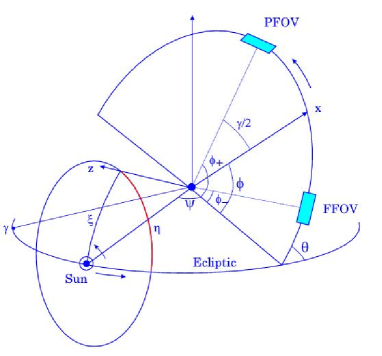
Figure 1: The nominal scanning law of Gaia. The spacecraft rotates around the $z-$axis in 6 hours so that the fovs sweep approximately a circle on the sky. The $z-$axis is constrained to move on a sun-centered cone of 50 degrees half-aperture with a period of 70 days, forcing the plane of scan to sway back and forth with inclinations between 40 to 140 deg. The axis of the cone follows the yearly solar motion.

2.2 The photometric fields of view

The Gaia payload is fitted with two main telescopes with an aperture of $1.4\times 0.5$ m², primarily dedicated to astrometry and full light photometry. On each field, several columns of ccds are covered with broad-band filters. This broad-band photometric field provides multi-colour, multi-epoch photometric measurements for each object observed in the astrometric field, for chromatic correction and astrophysical purposes. Four or five photometric bands should be implemented within each instrument with an integration time of $\sim 3.3$ s per ccd. A third telescope with a square entrance pupil of $0.5\times 0.5$ m² collects starlight for the spectrometer and the medium-band photometer.

3 Sequences of observation

Due to the combination of the quick spin motion over six hours and that of precession over 70 days coupled with the annual solar motion, the sampling of the epochs at which a particular object is measured is very peculiar and quite irregular. However, irregular does not mean random, and there are some basic recurring patterns which apply to each sequence. One must consider separately the succession of observations over period less than $\sim$ 1-2 day due to the repeated passages over few consecutive rotations of the satellite and are primarily governed by the spin and the focal plane layout, and the return in a particular direction after several weeks without observations, controlled by the precession motion. So a complete sequence divides itself naturally in succession of epochs, widely separated in time, in which there are a small number (between $\sim$ 1 to 10) of observations in the astrometric or photometric fields of view. For a regular sampling the ability to carry out accurate frequency analyses of variable stars depends on the succession of repeated observations over short time-scale, that is to say on sequences of successive revolutions separated by returns of the viewing direction to the same area of the sky. However for a purely random sampling one can obtain alias-free results even for frequencies much higher than the inverse of the smallest intervals between observations and one should not worry too much about the time gaps between successive observations. But Gaia sampling is obviously not perfectly regular but also falls short from a purely random sampling. This is something intermediate with regular patches over short time-scales repeating with much irregularity over longer time-scales. At the end the combination of the two interleaved sampling proved important to achieve an ambiguous and accurate frequency retrieval.

The variety of short term intervals likely to occur within a sequence of observations is given in Table 1. The highest temporal resolution is obtained by combining successive crossings in the MBP field with a photometric measurement obtained in the astrometric preceding field, leading to a minimum interval of 38 minutes.

Table 1: Fundamental sampling intervals following from the Gaia scanning law and from the location of the viewing directions. Transitions from an initial field to a final field are considered with the interval given in days. PFOV: preceding astrometric field of view, FFOV: following astrometric field of view, MBP: Medium band photometer field of view.

Initial field	Final field	Interval
		hours
PFOV	FFOV	1.78
PFOV	MBP	5.38
PFOV	PFOV	6.00
FVOV	MBP	3.60
FFOV	PFOV	4.22
FFOV	FFOV	6.00
MBP	PFOV	0.62
MBP	FFOV	2.40
MBP	MBP	6.00

3.1 Short term succession

3.1.1 Astrometric fields

Let a star be observed in the preceding astrometric field, at some reference time $t=0$. The star is located somewhere in the field of view of width $0.66$ degree in the cross-scan direction. We use a local rectangular frame with x-axis along the scan direction and y-axis in the transverse direction. Take the star image at the middle of the field for this reference time, that is to say $y=0$. Six hours later this viewing direction is back in nearly the same region of the sky. However the pole of the scan circle has moved by nearly 1 degree on the sky, and the ordinate of the star in the field can now be as large as 1 degree. In this case the star is no longer in the field of view and cannot be re-observed. On the other hand if the star happens to lie very close to one of the two stationary points of the scan circle (over a period of few days the scan of the sky can be described by the slow motion of a great circle, implying that there are two nodes on this circle which are stationary) the star has virtually not moved on the field and will be observed again after one revolution, and this situation could recur during four or five rotations of the satellite, supplying as many observations in the preceding fov.

Consider now the transition between the preceding and following astrometric fov’s. They are separated by 106 degrees, meaning that it takes 106 minutes to rotate from one field to the next. During this interval the apparent transverse motion of the star with respect to the scan circle is at most of 0.3 degrees. Therefore a star observed at a random position in the preceding field will be observed in the following field with a $\sim$ 0.5 probability. The average transverse motion being only $2/\pi\times 0.3=0.19$ degree, this makes the odds more favourable for the observations to be grouped at least by pair. With smaller transverse motion (star closer to the instantaneous node) one may have four or five successive pairs of observations, each separated by 0.25 day. During these crossings there are photometric measurements in full light and in the five broad band filters as well.

We can do a simple probabilistic modelling to assess the probability that an observation in a particular field is isolated (sequence of length 1) or followed by at least one observation in the next available field of view. It is reasonable to assume that the first observation of a sequence may occur at any ordinate in the field (this is a crude approximation, as the first observation of a sequence is more likely to occur near the upper or lower edge of the field). The chance of having the star observable in the next field depends on the transverse velocity and on the interval of time between the two fields. Let $V_{t}$ be the transverse velocity and $\Delta t$ the interval of time. One has $\Delta t=106$ minutes from preceding fov (pfov) to following fov (ffov), 254 mn from ffov to pfov and 360 mn = 0.25 day for one revolution. The transverse velocity depends very simply on the longitude $\phi$ of the optical axis on the instantaneous scan circle and takes the form $V_{t}=V_{\mbox{max}}\,\sin(\phi+\alpha)$ with $V_{\mbox{max}}=0.170$ deg/h and where $\phi$ is a fast moving angle (period of 6 h) and the phase $\alpha$ is a slow varying variable with a typical time-scale of 70 days. We call $\mathbf{X}$ the random variable $\mathbf{X}=1$ if the star is not re-observed after the first crossing at the start of a new epoch, and $\mathbf{X}=0$ for the opposite outcome. If $h$ is the transverse size of the field, it is easy to establish (see the Appendix) by conditioning the random variable to the transverse velocity and computing the expectation $\mbox{E}(\mbox{E}(\mathbf{X}|\mathbf{V_{t}}))$ that,

$$P(\mathbf{X}=1)=$$

$$\left\{\begin{array}[]{ccl}\frac{2}{\pi}\,\frac{1}{u}&\mbox{\ if \ }&u\geq 1\\[11.38109pt] \frac{2}{\pi}\,\frac{1}{u}\,\left(1-(1-u^{2})^{1/2}\right)+\frac{\pi-2\,\arcsin(u)}{\pi}&\mbox{\ if \ }&u\leq 1\end{array}\right.$$ (1)

where $u=h/V_{\mbox{max}}\,\Delta t$. When $u>1$ the transverse motion over $\Delta t$ is always less than the width of the fov while it can be larger otherwise when $u<1$. For the transitions between the preceding to following fov this yields a probability $P=0.71$ that more than one observation occurs and 0.32 for the transition between the following and preceding field, with the same assumption that the observation in the first field is the first of a sequence.

Table 2 gives the actual frequency of the different length of the sequence based on a simulation over 10 000 randomly distributed stars on the sky. The positions of these stars have been compared with the viewing directions over five years, thus producing for each star the time sampling in each field of view. The termination criterion for a continuous sequence of observations is activated when the interval between two successive observations is larger than few revolution periods of the satellite. A gap of 3 or 4 revolutions ($\sim 1$ day) may happen in a short time sequence in the passage from MBP transits to BBP transits as a result of the relative location of their respective detectors as shown in Fig. 2. From trials and errors we have found that a time gap between two successive observations larger than 2.5 days was a good signature to isolate short observing sequences from very different observing epochs. This means essentially that when one has a gap of 2.5 days without observation, the actual gap will be in practice much larger ($\sim 20-30$ days), with few exceptions well accounted for by the idiosyncrasies of the scanning law.

In the first two columns of Table 2, only the observations in the astrometric fields have been monitored and sequences starting with the preceding fov (sequences like P, PF, PFP, PFPF $\cdots$) or following fov (sequences like F, FP, FPF, FPFP, $\cdots$) are counted separately. They are not symmetrical, because the occurrence of a sequence pfov $\rightarrow$ ffov is more likely than the opposite sequence. The typical sequence comprises two observations (PF) in the first group, while sequences of unit length (F) are the most common in the second group. The average length of the sequences is 2.1 in the first case and 1.6 in the second. While the number of long sequences is small (less than one percent of the sequences longer than 10 observations), the length of the sequences can be very large and can reach 20 or 40 consecutive observations, meaning that the star is observed at regular interval for up to 5 days.

3.1.2 Astrometric and spectroscopic fields

We introduce now the field with the medium band filters (MBP fields of view). It is located ahead of the preceding field, at 38 degrees as depicted in Fig. 3 and comprises two subfields symmetrically placed with respect to the scan direction as shown in Fig. 2. Its vertical extension is much larger than the astrometric fields, meaning that the probability that a star is observed in this photometric field is higher than in the astrometric fovs. The average number of observations is just above 200 in the medium band photometer over the 5-year mission. The distribution with the ecliptic latitude (Fig. 4) displays the same symmetrical behaviour as for the observations with the broad band filters.

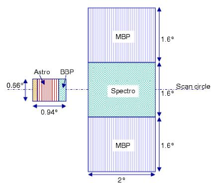
Figure 2: Relative size of the fields of view of Gaia. Many more field crossings arise in the medium band photometer (mbp) than in the broad band photometers (bbp) in the astrometric fields, as a result of the vertical extension.

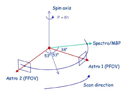
Figure 3: Relative positions of the viewing directions along the scan circle. MBP = Medium band photometry, PFOV (resp. FFOV) = preceding (resp. following) field of view.

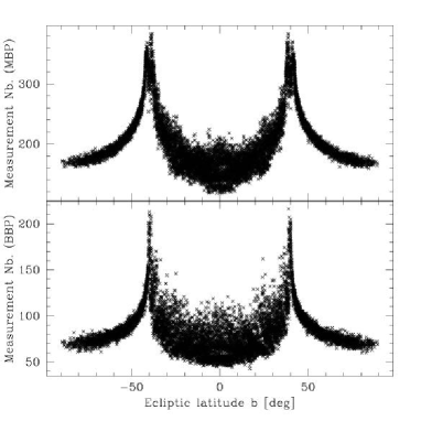
Figure 4: Number of measurements in MBP (top) and BBP (bottom) fields of view as function of ecliptic latitude ${b}$. The mean number of observations is 200 for the MBP and 80 for the BBP.

The transverse motion over one revolution is always smaller than the vertical extension of any of the two subfields, which implies that observations take place over at least two successive revolutions of the satellite. In fact, the average length of a sequence consists of 6-7 consecutive observations within less than a day, with measurements in every bandpass. In this case all the sequences but a handful start with an observation in the MBP field and a typical sequence is MMPFMM, meaning two MBP measurements followed by observations in the preceding and following astrometric fields and then again two in the MBP field. The probability distribution of the sequence lengths is given in the rightmost column of Table 2. Very long sequences of nearly 100 uninterrupted consecutive observations over $\sim$ 10 days may happen exceptionally.

The distribution of the short intervals when observations in the three photometric fields are combined is shown in Fig. 5. The most frequent interval is 0.25 days, corresponding to one spin period between two successive observations in the medium band photometer and accounts for 50 percent of the intervals. The origin of the other intervals can be read in Table 1, by adding in some instances one or two revolutions of 0.25 days.

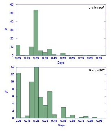
Figure 5: Frequency distribution of the intervals between consecutive observations performed at the same epoch in the three photometric fields of view. This indicates that the most common interval between paired observations is the 6 hours of the scan period. The lower panel is a close-up view of the overall distribution shown in the upper panel.

Table 2: Frequency distribution of the number of observations in continuous sequences. In the 2nd and 3rd columns only transits in the astrometric FOV are considered (that is to say in the BBP filters) while the last column includes also the MBP filters. The table gives the frequency of sequences of different lengths, according as the first field in the sequence is the preceding or following astrometric field of view (col 2 & 3), while for the MBP, due to the size and position of the detectors, all sequences start with few consecutive observations in MBP, followed by transits including only BBP and MBP, before additional crossings of the MBP.

	Sequence starts with
length	pfov	ffov	MBP
1	0.27	0.63	0.00
2	0.60	0.20	0.00
3	0.05	0.11	0.06
4	0.04	0.02	0.13
5	0.01	0.02	0.33
6	0.01	0.00	0.22
7	0.00	0.00	0.07
$>7$	0.01	0.01	0.19

3.2 Long term succession

The short term succession within an epoch is essentially driven by the relative position of the fields and the spin period, which control the time needed to rotate from one field to the next. The transverse motion which leads to the end of a sequence and later to the beginning of a new one is due to the slight displacement of the spin axis on the precession cone of $\sim$ 4 degrees per day. Therefore the return of an epoch of observation is primarily determined by the precession motion and the yearly solar motion on the ecliptic.

We have seen in the previous section, that the average length of a sequence in the astrometric fields only, is very close to two. With a total of $\sim$ 80 observations in total (Fig. 4), this gives about 40 epochs distributed over the 1800 days of the mission, or a typical interval between epochs of 45 days. If we take the combined observations in the two photometers instead, we have 280 observations and an average sequence of 6.5 observations, that is to say a return again every 45 days. However we have seen that the total number of observations per star is also function of the ecliptic latitude, as any other effect tied to the precessional motion. The actual number as a function of the latitude can only be obtained through a simulation with a fairly large number of stars.

The frequency distribution is shown in Fig. 6 for the ecliptic region, the intermediate latitude and the extended polar cap. These distributions are very informative, and indeed more relevant for the purpose of variable analysis than a weakly scattered distribution about the average interval would be. Below ${b}=40\degr$, there is quite an extensive coverage between 5 to 150 days, with two holes in the ranges 50–80 days and 100–130 days. At higher latitude, the scatter is less pronounced, with a smaller period between two epochs, meaning more observations. Clearly the period recovery of variable stars will depend, not strongly indeed, on the ecliptic latitude just because of the time sampling. The evaluation of this feature is the main object of the coming sections of this paper. A similar conclusion applies to the periods of spectroscopic binaries determined from the radial velocity measurements as found by Pourbaix & Jancart (2003).

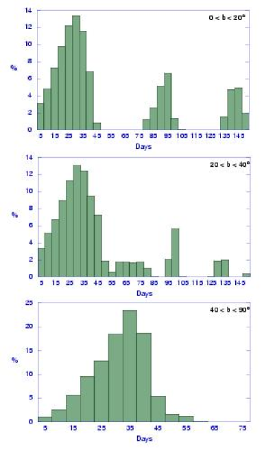
Figure 6: Frequency distribution (as a function of the ecliptic latitude) of the intervals of time between epochs of observations in the three photometric fields of view. The recurrence is primarily driven by a combination of the precessional motion of Gaia spin axis and the yearly solar motion.

4 Simulations

4.1 The time sampling

As said earlier a catalogue of 10 000 directions uniformly distributed has been produced. From the position and size of the different fields of view and the scanning law it was possible to sample the 1800 days of the mission and determine at any time which regions of the sky are observable by each instrument. When a star lies in a field, one computes then accurately the date of the crossing of the central line of the field, together with its ordinate and transverse velocity and the index of the field. Many refinements are used to speed up the runtime by eliminating quickly many of the stars not observable within $\sim$ a day. The output is finally re-organised to produce chronological time series for each of the 10 000 stars. This gives at the end a set of about 3 million observations scattered over 5 years. This file of realistic observing sequences is then the basis of the photometric simulation and the variability analysis.

The distribution of the number of individual observations (an observation at a particular date corresponds to the crossing of one field of view) is shown in Fig. 4 as a function of the ecliptic latitude for the $10\,000$ sources of the simulation. There is a strong dependence resulting from the scanning law, with mid-latitude region over observed compared to the mean, while the ecliptic region is observed less frequently than the average. The same pattern is common to the main astrometric field, which includes the BBP filters, and to the MBP field. However due to the larger across-scan extension of the latter, about twice as many observations are made in the latter field. This appears clearly in Fig. 7 which displays the frequency distribution of the number of observations in the same two fields of view. The scatter in each field is significant with variation from 40 to 150 in the astrometric fields and 100 to 300 in the MBP field.

Figure 7: Histograms of the number of measurements for the astro-fields (both following and preceding) and for the MBP field. The extended scatter towards the largest values comes from the observations around $40\degr$ of ecliptic latitude.

Quite as important as the number of observations is the number of different epochs at which the signal is sampled. The observations are clustered into small groups of $\sim$ 2 to 10 observations within a day, before a new cluster shows itself after several weeks. The number of epochs based on the same simulation plotted in Fig. 8 shows that there are essentially two regimes: the ecliptic zone with $\pm 30\degr$ with about 30 observational epochs over the five years and the region of upper ecliptic latitude, above $40\degr$, with $\sim 50$ different epochs. This feature impacts significantly on the variability analysis probably more than the total number of observations, since it is directly related to the ability to recover the characteristics of periodic phenomena. Even after a normalization over the $S/N$ values, there should remain a systematic effect with the ecliptic latitude.

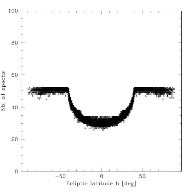
Figure 8: Number of clustered groups as function of ecliptic latitude ${b}$. The pattern is much simpler than that for the total number of transits (Fig. 4), with only two regimes : low and high ecliptic latitude.

4.2 The photometric signal

For each star one generates the photometric variability, modelled by a simple sinusoidal signal with one frequency. More complex light curves have been tested with several harmonics representing non-sinusoidal oscillations of pulsating variables or eclipsing binaries without affecting the main conclusions of this study, although the case of the eclipsing binaries is the source of specific problems. Therefore our baseline simulated signal has the form,

$$s(t)=S_{0}+A\sin(2\pi\nu t+\phi)+\mbox{noise}$$

where $A$ is the amplitude of the variability, $\nu$ the frequency, $\phi$ the phase. One should note that variable stars are usually characterised by the amplitude of variability, that is to say by the peak to peak amplitude $2*A$. The noise added to the deterministic signal is a Gaussian random variable of zero mean with a standard deviation determined by the signal-to-noise ratio of each experiment. Although we have also experimented with multi-periodic signals, the results presented here refer to purely periodic variables.

All the simulations are scaled by the $S/N$ ratio (defined here as $A/$noise). This is a convenient parameter which makes our results independent of the star magnitude. However as a result of the systematic variation of the number of observations with the ecliptic latitude, the dominant effect in the variability analysis beyond the $S/N$ ratio, is the ecliptic latitude. In order to avoid this bias, we have used a normalised definition of the signal-to-noise ratio, by dividing the single observation noise in $S/N$ by $n^{1/2}$. More precisely we have,

$$\chi=S/N\times\sqrt{n/80}$$ (2)

so that $\chi\sim 1$ for an average observation with $S/N=1$, while at ${b}\sim 40\degr$, $\chi=1$ is equivalent to $S/N\sim 0.65$. Therefore any remaining effect with the ecliptic latitude will arise more from the time sampling than from the systematic difference in the number of observations.

Simulated variables are generated for a grid of frequencies and $\chi$. For each point of this grid, and for all the sources a period search is performed on the signal, without any a priori information, using primarily an optimised version of the Lomb-Scargle algorithm [Press et al., 1992] or a frequency analysis based on orthogonal decomposition developed by one of us (FM). The rate of success in the period retrieval for every grid point is the main output of the program. Regarding the size of the computation, we have sampled about 10 periods (from the slowest Miras to the shortest pulsating variable with periods of few hours) and between 3 and 5 values of the normalised $S/N$. Each of the 10 000 stars (or 5000 for the runs limited to one hemisphere) has been used 5 times, with independent random noise on the observations. This gives in total 50 000 period searches for every grid point. In total the number of computed ”periodograms” reaches nearly 1.4 million.

5 Results

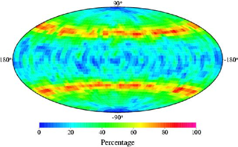
Figure 9: Rate of correct detections for $S/N=0.75$ and a single period of 0.2 days, using only the astrometric fields. We are here in a range of small signal-to-noise ratio. For certain regions, the rate reaches nearly 0% and for other regions where the number of measurements is high, it reaches nearly 100%. The small effects in longitude follow from the non-uniform coverage observation density as of function of longitude over 5 years.

5.1 Rate of detection

Results consist primarily of correct rate of detection as a function of the period, the signal-to-noise ratio and the position on the sky, this as a result of the inhomogeneous time sampling of Gaia. Fig. 9 gives for a single grid point ($P=0.2$ day and the unnormalised $S/N=0.75$) the sky distribution of the correct rate of period retrieval. The main pattern reproduces the scatter of the number of observations with the ecliptic latitude, which has been subsequently eliminated with the normalised $S/N$. In the range of latitude around $40\degr$ the rate is close to $80$ percent, and between $20$ and $50$ percent outside this area. The rate falls off very quickly with lower signal-to-noise ratio, but on the other hand grows quickly to $100$ percent for $S/N>1.5$.

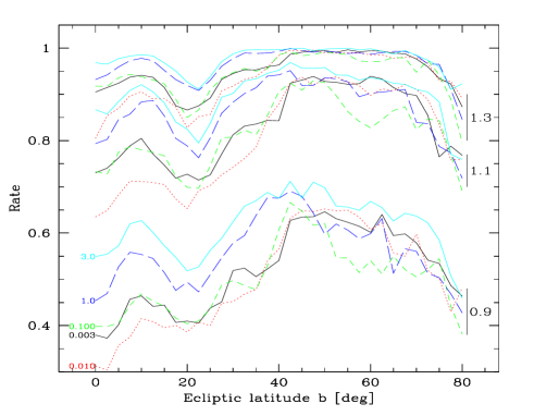
Figure 10: Rate of correct detection for normalised signal-to-noise ratios $\chi$ (written on the right) and frequencies [cycle/day] (written on the left for the normalised signal-to-noise ratio of 0.9, the same colour/gray scale and line type are applied for the higher signal-to-noise ratios).

Since there are only small secondary modulations with the ecliptic longitude, one can perform one dimensional analyses by looking at the dependence with the ecliptic latitude for various grid-points. Results are shown in Fig. 10. There are three sets of curves for $\chi=0.9,1.1,1.3$ and different periods (8h, 1, 10, 100 and 330 days).

• It is clear, that despite the normalisation of the $S/N$, the effect with the ecliptic latitude has not fully vanished, indicating an influence of the number of epochs (the number of clusters of observations separated by few weeks shown in Fig. 8). There is a systematic loss in the period recovery around ${b}\simeq 20\degr$, not easily understood at the moment.

• The rate of correct recovery grows quickly to $100$ percent, with normalised $S/N\geq 1.5$.

• Although the scatter is large, it seems that the shorter periods ($<1$ day) are better recovered than the larger periods. However the difference is not conspicuous and this comes as a surprising (and welcome) result, as it was thought that very short periods would be very difficult to recover.

5.2 Aliasing and false periods

With irregular sampling, and within the range of periods analysed here, one should not expect too much aliasing [Eyer & Bartholdi, 1999], since the somewhat randomness of the sampling limits the building up of coherent signature at regularly spaced frequencies. However, at low signal-to-noise levels, the recovery rate is low, and the search program may end up in a normal exit with no periodic signal found (the favourable outcome) or with the identification of a period (possibly wrong), without warning. It is then of interest to look at what kind of periods are found as a function of the true period. This is illustrated in Fig. 11 for the BBP (same field as the astrometric detector) (top) and the MBP fields (bottom). The simulated variable has a period of one day and $S/N=0.75$ in this example. In the BBP, when the period is not recovered (about half of the cases tested) the final erroneous frequency can be almost anything, with a higher probability to frequencies of 11 and 13 cycles per day, coming from the convolution with the spectrum of the observing window. So, unless further assumptions, there is no way to decide from the output of the period search whether the period found is correct, although a significance level is easily produced and could be used as a warning, but not as a measurement of the uncertainty of the period. In the case of the MBP, aliased results are clearly visible, regularly spaced with $\delta\nu=2$ cycles/day, corresponding to half of the satellite spin frequency (period of 6 hours). This comes from successive observations regularly sampled every revolution within a cluster of observations, responsible for the aliasing and leading to a wrong determination of the period. This again cannot be avoided with the present design of the instrument, but fortunately limited to those observations with low SNR.

Figure 11: Example of terminal frequencies for an initial signal of $S/N=0.75$ and frequency $\nu=1.000$. It reflects the pattern of individual periodogram, which bears the signature of the spectral window.

6 Conclusion

In this paper we have investigated the retrieval of periods of variable stars from observations to be carried out during the Gaia mission. We have found, that with adequate frequency analysis algorithms, one can recover period of regular variable stars even with signal-to-noise ratio around unity. It is also shown that the very irregular time sampling expected from Gaia allows to determine frequencies much higher than the upper frequency estimated from a straightforward evaluation of the Nyquist boundary (cf. Eyer & Bartholdi 1999), and with virtually no aliasing. These two features are very good news for the preparation, and subsequent scientific exploitation, of the mission.

However, from this investigation we have noted that the frequency analysis without initial assumption on the frequency range may be very demanding in term of computer resources, hardly compatible with the goal of analysing from scratch $\sim 10^{8}$ sources. Therefore a major effort is needed during this preparatory phase to develop optimised software, to estimate quickly and efficiently possible periods or ranges of periods, before a thorough and accurate search can be launched on a well bounded frequency range. An estimate of the level of significance of each peak height should be also a built-in feature, alongside the possibility of searching for harmonics or a second independent period.

7 Acknowledgements

We would like to thank Michel Grenon for interesting discussions and Floor van Leeuwen for his valuable comments on the article.

Appendix : Derivation of equation 1

Let a star observed in one field and crossing the field in the along-scan direction at the ordinate $y$. The field height is $h$ and $0<y<h$ during the transit. This crossing may happen at any ordinate with a uniform probability, so that $P(\bf{Y}<y)=y/h$. After an interval of time $\Delta t$ (one of the possible intervals between the preceding and following fields listed in Table 1) the rotation of the satellite has brought the line of sight of the second field in the same direction and the star may be observed again, provided its transverse motion during $\Delta t$ has not been too large. Mathematically the star cannot be observed again if $y+V_{t}\ \Delta t>h$, meaning that its new ordinate is larger than the field height (we have restricted to the case $V_{t}>0$ to simplify the discussion, but this does not alter the final result for symmetry reasons). Therefore the probability that the star is not observed in the second field when the transverse velocity is $V_{t}$ is,

$$P(({\bf{X=1}})|V_{t})=$$

$$\left\{\begin{array}[]{lcl}1&\mbox{\ if \ }&V_{t}\ \Delta t\geq h\\[11.38109pt] P({\bf{Y}}>h-V_{t}\,\Delta t)=\frac{V_{t}\,\Delta t}{h}&\mbox{\ if \ }&V_{t}\ \Delta t\leq h\end{array}\right.$$

In the first case the transverse velocity is large enough for the transverse motion during $\Delta t$ to be greater than the field width. In the second case there exists a region in the initial field of view where even after the time $\Delta t$ the ordinate of the star is still less than the field width. The above probabilities are conditioned on the transverse velocity $V_{t}$ and one must now introduce its random distribution. Assuming that the star can be anywhere on the scan circle with a uniform probability, one has $V_{t}=V_{\mbox{max}}\ \sin(\phi)$ where the maximum velocity $V_{\mbox{max}}=0.170$ deg/h and $\phi$ is uniformly distributed between $0$ and $2\pi$. The final probability is just the average of the conditional probability over the distribution of the transverse velocity (restricted here to the positive values). The case when $V_{\mbox{max}}\ \Delta t/h\leq 1$ is very simple with

$$P({\bf{X=1}})=\frac{2}{\pi}\,\frac{V_{\mbox{max}}\ \Delta t}{h}\ \int_{0}^{\pi/2}\,\sin\phi\,d\phi=\frac{2}{\pi}\,\frac{V_{\mbox{max}}\ \Delta t}{h}$$

In the second case the integration extends up to $\phi_{m}$ such that $V_{\mbox{max}}\ \Delta t\sin\phi_{m}=h$, or $\phi_{m}=\arcsin(h/V_{\mbox{max}}\ \Delta t)$, and beyond this angle the conditional probability is one. This yields for $V_{\mbox{max}}\ \Delta t/h\geq 1$,

$$P({\bf{X=1}})=\frac{2}{\pi}\,\frac{V_{\mbox{max}}\ \Delta t}{h}\ \int_{0}^{\phi_{m}}\,\sin\phi\,d\phi+\frac{2}{\pi}\ \int_{\phi_{m}}^{\pi/2}\,d\phi$$

giving with $u=h/(V_{\mbox{max}}\ \Delta t)$ (hence $u<1$ here),

$$P({\bf{X=1}})=\frac{2}{\pi}\,\frac{1}{u}\left[1-\left(1-u^{2}\right)^{1/2}\right]+\left[1-\frac{2}{\pi}\,\arcsin u\right]$$

which is the same as Eq. 1.

References

- [Eyer & Bartholdi, 1999] Eyer, L., & Bartholdi, P. 1999, A&AS, 135, 1
- [Eyer & Cuypers, 2000] Eyer, L., Cuypers, J. 2000, in ASP Conf. Ser. 203, The Impact of Large-Scale Surveys on Pulsating Star Research, ed. L. Szabados, & D. W. Kurtz, Proc IAU Colloq. 176, 71
- [Eyer & Grenon, 1997] Eyer, L., Grenon, M. 1997, ESA SP-402, 467
- [Jordi, 2003] Jordi, C., et al. 2003, in Gaia Spectroscopy, Science and Technology, 209–220, ASP Conf. Ser. 298, ed. U. Munari
- [Mignard, 2001] Mignard, F. 2001, A practical scanning law for Gaia simulations, Technical Note GAIA_FM_010
- [Perryman et al., 2001] Perryman, M.A.C., de Boer, K.S., Gilmore, G., et al. 2001, A&A, 369, 339
- [Pourbaix & Jancart 2003] Pourbaix, D., & Jancart, S. 2003, in ASP Conf. Ser. 298, Gaia Spectroscopy, Science and Technology, ed. U. Munari, 345
- [Press et al., 1992] Press, W. H., Teukolsky, S. A., Vetterling, W. T., Flannery, B. P. 1992, Numerical Recipes in Fortran. Cambridge University Press