Tracking Dark Energy with the ISW effect: short and long-term predictions

Abstract

We present an analysis of the constraining power of future measurements of the Integrated Sachs-Wolfe (ISW) effect on models of the equation of state of dark energy as a function of redshift, $w(z)$. To achieve this, we employ a new parameterization of $w$, which utilizes the mean value of $w(z)$ ($\left<w\right>$) as an explicit parameter. This helps to separate the information contained in the estimation of the distance to the last scattering surface (from the CMB) from the information contained in the ISW effect. We then use Fisher analysis to forecast the expected uncertainties in the measured parameters from future ISW observations for two models of dark energy with very different time evolution properties. For example, we demonstrate that the cross–correlation of Planck CMB data and LSST galaxy catalogs will provide competitive constraints on $w(z)$, compared to a SNAP–like SNe project, for models of dark energy with a rapidly changing equation of state (e.g. “Kink” models). Our work confirms that, while SNe measurements are more suitable for constraining variations in $w(z)$ at low redshift, the ISW effect can provide important independent constraints on $w(z)$ at high $z$.

I Introduction

There is now a substantial amount of observational evidence that the universe is dominated by a dark component which is causing its expansion rate to accelerate. The analysis of the Cosmic Microwave Background (CMB) anisotropy power spectra Spergel combined with results from large scale structure (LSS) surveys 2dFSDSS strongly suggest that about $70\%$ of the energy in the universe is in an exotic form of matter which we refer to as dark energy (DE). Measurements of the luminosity distance to Supernova Type Ia (SNIa) independently confirm these conclusions by showing that high redshift supernovae are dimmer than in a matter dominated universe RiessPerl .

Further evidence, which has recently become available, is the detection of the Integrated Sachs-Wolfe (ISW) effect using the CMB/LSS cross-correlation xray ; nolta ; fosalba ; scranton ; afshordi03 . This evidence is complementary in nature to the SNIa data. Rather than probing the overall expansion of the universe, it detects the slow down in the growth of density perturbations that occurs when the universe ceases to be matter dominated. CMB photons traveling to us from the surface of last scattering blueshift and redshift as they fall into and climb out of gravitational potentials along their paths. During matter domination, the large scale potentials remain constant in time, hence the blueshift and the redshift exactly cancel each other out. However, any deviation from a constant total equation of state results in a time variation of the potentials and a net change in the photon energy. This is observed as an additional CMB temperature anisotropy, which is the ISW effect Sachs .

Detecting the ISW effect from measurements of CMB temperature anisotropy alone is not feasible because the signal is hard to separate from the primordial anisotropy from the last scattering surface. To circumvent this, it was proposed to correlate the CMB temperature maps with the local distribution of matter turok96 . The cross-correlation arises from CMB anisotropies produced after the cosmic structures were formed. On large angular scales the cross-correlation signal is dominated by the ISW effect, while at small angles an additional contribution comes from the Sunyaev-Zel‘dovich effect Sun ; Peiris .

The cosmological constant $\Lambda$ is the simplest model of dark energy that provides a satisfactory fit to the existing data. Despite the success of the concordance $\Lambda$ cold dark matter scenario ($\Lambda$CDM), it is difficult to explain why the cosmological constant value is so extremely small compared to the expectations of particle physics without involving anthropic selection anthro . On the other hand, the observations are also consistent with an evolving dark energy, such as Quintessence models where the dark energy originates from a scalar field wetterich ; peebles ; caldwell98 . Establishing whether the dark energy is constant or evolving is one of the main challenges for modern cosmology. In the Friedmann-Robertson-Walker (FRW) universe the evolution of dark energy is completely determined by its equation of state, which is defined as the ratio of pressure to energy density: $w\equiv p/\rho$. For scalar field Quintessence, the sound speed is unity and $w$ determines the clustering properties of DE. Depending on the model $w$ can be constant or change with time. Models with $w\neq-1$ correspond to evolving DE, while $w=-1$ corresponds to $\Lambda$.

The time dependence of the dark energy equation has been constrained by fitting various forms of $w(z)$ to the SNIa data, often in combination with CMB and the LSS measurements Wang ; Corasetal04 ; Hannestad04 ; Bruce04 ; Rapetti ; jassal05 . However the data are not accurate enough to distinguish between the cosmological constant and many forms of dynamical dark energy. Moreover degeneracies between dark energy parameters strongly limit the possibility to test whether $w$ is constant or not.

As we shall describe in this paper, the CMB/LSS correlation can provide another probe of the evolution of $w(z)$. The sensitivity of the cross-correlation to the dark energy evolution has previously been investigated in GPV04 ; Levon04 . In this paper we study constraints expected from correlating surveys such as DES and LSST with the CMB data. We introduce a novel way of parameterizing $w(z)$ that has the average $\left<w\right>$ (eq. (3)) as an explicit parameter. This helps to separate information contained in the estimate of the distance to last scattering from that in the ISW contribution. We then proceed to show that the cross-correlation, in the absence of errors, is more sensitive to the details of the high redshift evolution of $w(z)$ than other available observables. This sensitivity, however, is off-set by large statistical errors due to a large primordial contribution to the CMB signal. We forecast the expected uncertainties in DE parameters (using two different models) extracted from CMB/LSS correlation that will be possible in the next five years (WMAP/DES) and in the next ten years (Planck/LSST). We also calculate corresponding constraints from the SNe data (SNLS in short term and SNAP in long term). We find that in long term, cross-correlation can provide competitive constraints on the evolution of $w(z)$.

The paper is organized as follows. In Section II we discuss the dark energy modeling and the details of the calculations. Section III describes the observations considered in the paper. In Section IV we discuss some advantages of including the cross correlation information and give the resulting parameter constraints. Finally in Section V we present our conclusions.

II Formalism and methods

II.1 Dark energy model

Many models of dark energy have been proposed: cosmological constant ($\Lambda$), Quintessence, k-essence, tangled defects, etc. For simplicity, we will focus on quintessence based models where the dark energy arises from a scalar field currently slow-rolling down a potential, which is effectively inflation occurring at late times. Perturbations in the dark energy are easily incorporated in such models, and the sound speed is typically of order the speed of light.

The shape of the potential, which determines the evolution of the dark energy, is generally a free function. This makes it difficult to predict the time dependence of the DE equation of state, so one is potentially left with constraining a completely arbitrary function of redshift. The problem must be simplified by considering some parameterization of the function $w(z)$. Several parameterizations have been suggested in a vast literature, but any resulting constraints are very sensitive to the choice of parameterization. For instance it was shown in maor01 that fitting a constant $w$ will tend to favor lower negative values if the DE equation of state is time dependent. Even two-parameter Taylor expansions are too simplistic, resulting in a strong dependence on the assumed priors and generally biased against dynamical models Wang ; Bruce04 ; Taxil04 .

One of the most popular two-parameter formulae is the linear change in the scale factor $a=(1+z)^{-1}$ PolarskiLinder given by,

$$w(a)=w_{0}+(a-1)\delta_{w}\ ,$$ (1)

where $w_{0}=w_{Q}({\rm today})$ and $w_{m}=w_{0}+\delta_{w}$ being the value at some early time, such as the radiation-matter equality. From eq. (1) it appears evident that with two parameters one can fix the value of the equation of state today and at high redshift, but the time evolution between the two extremes cannot be changed (i.e. $dw/da={\rm const}.$). As consequence of this, a linear expansion cannot allow for rapid variation in the equation of state and particularly in the case of Quintessence, for which $w_{Q}>-1$, this bias will tend to favor small values of $\delta_{w}$. Despite these potential problems, eq. (1) has become a common tool of testing the capability of future experiments to constrain DE models (see UISLH ). Due to its wide use in the literature, we will consider this parameterization here to help the comparison of our results with previous works. We shall refer to it as Model I.

In order to avoid the pitfalls introduced by the Taylor expansion we also consider a phenomenological approach and model $w(z)$ according to some minimal requirements, which are: 1) the form of $w(z)$ depends on a minimal number of parameters which are of simple physical interpretation, 2) the parameterization is not biased against any particular time behavior and can account for both rapid (large) or slow (small) variation of the equation of state, 3) the parameterization reproduces the evolution of several proposed models of DE such as Quintessence. In this regard, a general formula constructed to follow these guidelines was proposed in brucemeta ; corased and is usually referred to as the “Kink” model Corasetal04 .

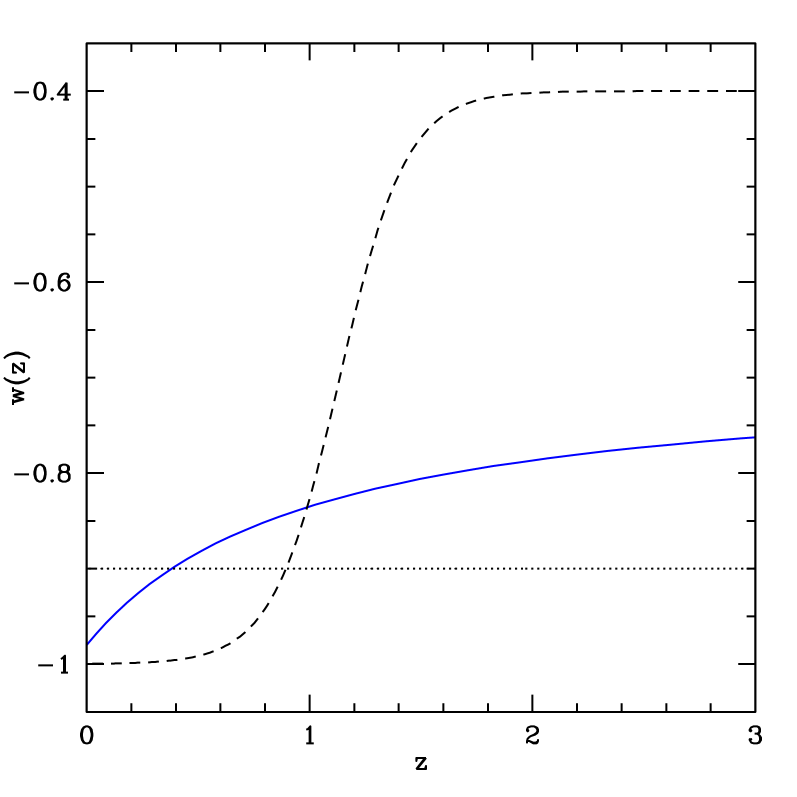
Figure 1: The equation of state as a function of redshift for the two fiducial models considered in the paper. Model I (blue solid line) and Model II (black dash line) have the same weighted average $\left<w\right>=-0.9$ (the dotted line) defined in eq. (3).

Within the class of the Kink models we consider a unique new parameterization. We start with the functional form

$$w(z)=\frac{w_{+}+w_{-}}{2}+\frac{w_{+}-w_{-}}{2}\ {\rm tanh}\left[{z-z_{T}\over\Delta_{z}}\right]\ ,$$ (2)

which describes a transition from $w_{+}$ for $z\rightarrow+\infty$, to $w_{-}$ for $z\rightarrow-\infty$, with parameters $\Delta_{z}$ and $z_{T}$ describing the width and the central redshift of the transition. The novelty is in using the average equation of state ($\left<w\right>$) as an explicit parameter, where $\left<w\right>$ is defined as

$$\left<w\right>\equiv{\int_{a_{\rm LS}}^{1}da\ w(a)\ \Omega_{D}(a)\over\int_{a_{\rm LS}}^{1}da\ \Omega_{D}(a)}\ .$$ (3)

Here $a$ is the scale factor ($a=1$ today), $a_{\rm LS}$ is the scale factor at the surface of last scattering and $\Omega_{D}(a)$ is the ratio of the DE energy density to the critical density. It is well known huey99 ; dave02 that on small scales the CMB temperature anisotropy spectra are insensitive to the details of $w(z)$ except for its average value as defined in eq. (3). Specifying $\left<w\right>$ roughly fixes the distance to the last scattering surface saini03 , which determines positions of the acoustic peaks in the CMB temperature anisotropy spectrum. The CMB temperature data, combined with a prior knowledge of $H_{0}$ and under the assumption that the universe is flat, is capable of constraining the value of $\left<w\right>$ with a very high accuracy. By explicitly specifying $\left<w\right>$ we preserve the information that would be obtained from fitting a constant $w$ to the CMB, while still allowing for a varying $w(z)$. Hence, a direct control on the value $\left<w\right>$ allows us to reduce the four dimensional parameter space to a much smaller observationally allowed region, which corresponds to a narrow range of possible values of $\left<w\right>$.

Note that for $\left<w\right>$ close to $-1$, as favored by the data, most choices of $\Delta_{w}$ would lead to $w(z)$ changing between $-1$ and $-1+|\Delta_{w}|$, where $\Delta_{w}=w_{-}-w_{+}$. Also note that in a large class of quintessence models either $w_{+}$ or $w_{-}$ is $-1$. This is the case when the scalar field is initially in a slow-roll regime ($w_{+}=-1$) as in, e.g., the Doomsday model Linde86 ; GV00 . Similarly for tracker models, where the quintessence field starts tracking the background component and evolves at late time settling to a minimum of its potential (i. e. $w_{-}=-1$) Trackers . Hence, fixing the value of either $w_{-}$ or $w_{+}$ to $-1$ is physically and observationally motivated and allows us to reduce the number of parameters in eq. (2) from four to three.

Thus, instead of using the four parameters of eq. (2), $w_{+}$, $w_{-}$, $z_{T}$ and $\Delta_{z}$, we use three parameters: $\left<w\right>$, $\Delta_{w}$ and $\Delta_{z}$. Here, $z_{T}$ is chosen to reproduce the desired value of $\left<w\right>$. (Alternatively, we could explicitly specify $z_{T}$ and use eq. (3) to find the corresponding value of $\Delta_{z}$.) Since we are primarily interested in determining whether $w(z)$ is varying or constant, $\Delta_{w}$ is the main parameter of interest. The role of the third parameter, $z_{T}$ or $\Delta_{z}$, is only to allow for sufficient freedom in the ansatz. In this paper, we will stay with the choice of $\left<w\right>$, $\Delta_{w}$ and $\Delta_{z}$ and refer to this parameterization as our Model II.

Representative plots of $w(z)$ versus $z$ for Model I and Model II are shown in Fig. 1.

II.2 Temperature and density correlations

The CMB temperature anisotropy due to the ISW effect can be written as

$${\delta T(\hat{\bf n})\over\bar{T}}=\int_{\eta_{m}}^{\eta_{0}}d\eta\ \left(\dot{\Phi}\left[(\eta_{0}-\eta)\hat{\bf n},\eta\right]-\dot{\Psi}\left[(\eta_{0}-\eta)\hat{\bf n},\eta\right]\right),$$ (4)

where $\hat{\bf n}$ is a direction on the sky, $\eta$ is the conformal time, $\eta_{m}$ is some initial time far into the matter era, $\eta_{0}$ is the time today, $\Phi$ and $\Psi$ are the gravitational potentials in the Newtonian gauge, and the dot denotes differentiation with respect to $\eta$.

The ISW temperature anisotropy can be correlated with the distribution of galaxies on the sky using,

$$\delta_{g}(\hat{\bf n})={{N}(\hat{\bf n})-\bar{N}\over\bar{N}}$$ (5)

where $\delta_{g}(\hat{\bf n})$ is the overdensity of galaxies in the direction $\hat{\bf n}$, $N(\hat{\bf n})$ is the number of galaxies in the pixel corresponding to the direction $\hat{\bf n}$, and $\bar{N}$ is the mean number of galaxies per pixel. We assume here that we sample galaxies in a fixed redshift region, characterized by a normalized galaxy selection function, $W_{g}(z)$. For simplicity, we initially consider a single selection function, but below we consider correlations arising between different redshift bins as well.

The galaxy number overdensity $\delta_{g}(\hat{\bf n})$ is assumed to be tracing the cold dark matter (CDM) density contrast $\delta_{c}(\hat{\bf n})$ via

$$\delta_{g}(\hat{\bf n})=b_{g}\delta_{c}(\hat{\bf n}),$$ (6)

where $b_{g}$ is the linear galaxy bias, which is possibly redshift dependent. The CDM density contrast can be written as an integral over conformal time,

$$\delta_{c}(\hat{\bf n})=\int_{\eta_{m}}^{\eta_{0}}d\eta\ {dz\over d\eta}\ W_{g}(z(\eta))\ {\delta_{c}}((\eta_{0}-\eta)\hat{\bf n},\eta),$$ (7)

where ${\delta_{c}}({\bf x},\eta)$ is the three-dimensional density contrast and is directly related to the gravitational potentials.

We are interested in calculating the cross-correlation function

$$X(\theta)\equiv X(|\hat{\bf n}_{1}-\hat{\bf n}_{2}|)\equiv\left\langle{\delta T^{\rm ISW}\over\bar{T}}(\hat{\bf n}_{1})\delta_{g}(\hat{\bf n}_{2})\right\rangle\ ,$$ (8)

where the angular brackets denote ensemble averaging and $\theta$ is the angle between directions $\hat{\bf n}_{1}$ and $\hat{\bf n}_{2}$. Calculations are often simplified when $X(\theta)$ is decomposed into a Legendre series,

$$X(\theta)=\sum_{l=2}^{\infty}{2\ell+1\over 4\pi}X_{\ell}P_{\ell}({\rm cos}\ \theta)\ .$$ (9)

The coefficients $X_{\ell}$ can be evaluated using GPV04 :

$$X_{\ell}=4\pi{9\over 25}\int{dk\over k}\ \Delta_{\cal R}(k)\ \Delta^{\mathrm{ISW}}_{\ell}(k)\ M_{\ell}(k)\ ,$$ (10)

where $k$ is the wave-number, $\Delta_{\cal R}^{2}(k)$ is the primordial curvature power spectrum, and functions $\Delta^{\mathrm{ISW}}_{\ell}(k)$ and $M_{\ell}(k)$ are defined as

$$\Delta^{\mathrm{ISW}}_{\ell}(k) = \int_{\eta_{k}}^{\eta_{0}}d\eta\ j_{\ell}(k[\eta-\eta_{0}])$$

$$\times (c_{\Phi\Psi}\dot{\phi}(k,\eta)-\dot{\psi}(k,\eta))$$

$$M_{\ell}(k) = b_{g}c_{\delta\Psi}\int_{\eta_{k}}^{\eta_{0}}d\eta\ j_{\ell}(k[\eta-\eta_{0}])$$ (11)

$$\times \dot{z}W_{g}(z(\eta))\delta(k,\eta)\ .$$

In the above, the integration starts at an early time $\eta_{k}$, when a given mode $k$ is well-outside the horizon, $j_{l}(\cdot)$ are the spherical Bessel functions, $\dot{\phi}(k,\eta)$, $\dot{\psi}(k,\eta)$ and $\delta(k,\eta)$ are the evolution functions defined in GPV04 along with the numerical coefficients $c_{\Phi\Psi}$ and $c_{\delta\Psi}$:

$$c_{\delta\Psi}\equiv{\delta\over\Psi}=-{3\over 2}\ ,\ c_{\Phi\Psi}\equiv{\Phi\over\Psi}=-\left(1+{2\over 5}R_{\nu}\right)\ ,$$ (12)

where $R_{\nu}\equiv\rho_{\nu}/(\rho_{\gamma}+\rho_{\nu})$ and $\rho_{\gamma}$ and $\rho_{\nu}$ are the photon and relativistic neutrino densities.

Above we have considered the correlations between the CMB and a sample of galaxies defined by a single galaxy selection function. Future surveys will enable us to separate galaxies into many redshift slices with photometric redshift slices (bins), and we can consider separate correlations with each of the slices, $X^{i}_{\ell}$. We calculate these as above using the different selection functions, $W_{g}^{i}(z)$, each of which has a corresponding weighting function $M_{\ell}^{i}(k)$. For each bin, we consider a different possible bias factor $b^{i}_{g}$, but as we discuss in Section IV.2, these can be determined sufficiently well by the observations of the galaxy-galaxy correlation functions.

The galaxy-galaxy correlations are evaluated in a similar way. We have many correlation functions $\omega^{(i,j)}(\theta)$, corresponding to correlations between all possible redshift bins labeled by indices $(i,j)$. Similarly to eq. (10), the Legendre coefficients of these correlations are given by

$$\omega^{(i,j)}_{\ell}=4\pi{9\over 25}\int{dk\over k}\ \Delta^{2}_{\cal R}\ M^{i}_{\ell}(k)M^{j}_{\ell}(k)\ .$$ (13)

The full CMB auto-correlation $C^{TT}_{\ell}$ contains the primary anisotropy from the last scattering surface as well as contributions from the ISW, the SZ and other effects:

$$C^{TT}_{\ell}=C^{\rm LS}_{\ell}+C^{\rm ISW}_{\ell}+C^{\rm SZ}_{\ell}+...\ .$$ (14)

The uncorrelated anisotropies from the last scattering surface dominate the noise in the cross correlation detection. The ISW contribution dominates the galaxy-CMB cross-correlation on large scales (where the signal is strongest), while the SZ effect is anti-correlated at WMAP frequencies and affects only the small angular scales fosalba . In principle the SZ signal can be eliminated by smoothing the CMB maps on scales smaller than the typical angular size of a cluster ( $1^{\circ}$), therefore we will not include the SZ in our analysis.

We evaluate the CMB/LSS correlation coefficients $X^{i}_{\ell}$, as well as all other relevant spectra, using an appropriately modified version of CMBFAST cmbfast . For all models, we assume a flat universe with adiabatic initial conditions for all particle species, including the Quintessence.

II.3 Fisher matrices

We use the usual Fisher method fisher for parameter estimation forecasts to study the potential of the CMB/LSS cross-correlation for dark energy constraints. We assume that the universe has evolved from adiabatic initial conditions with a nearly scale-invariant spectrum of density fluctuation, negligible tensor component and no massive neutrinos. It is also assumed to be flat with a Quintessence field parameterized by $w(z)$. In addition to the dark energy parameters $[w_{0}$,$\delta_{w}$] of Model I or [$\left<w\right>$,$\Delta_{w}$,$\Delta_{z}$] of Model II, our parameter space ${p_{\alpha}}$ includes the matter fraction of total energy density $\Omega_{M}$, the Hubble parameter $h$, the baryon density $\omega_{b}=\Omega_{b}h^{2}$, the reionization optical depth $\tau$, the scalar spectral index $n_{s}$ and the amplitude of the initial power spectrum $A_{s}$. In total, we have $8$ parameters for Model I and $9$ parameters for Model II. In addition, for the SNe analysis, we account for $M$ – the intrinsic supernova magnitude. Cross-correlation parameters also include the bias factors for each photometric bin, as described in Section IV.2.

The cross-correlation Fisher matrix can be written as

$$F^{X}_{\alpha,\beta}=f_{\rm sky}\sum_{\ell=\ell_{\rm min}}^{\ell_{X}}\sum_{i,j}{\partial X^{i}_{\ell}\over\partial p_{\alpha}}{\rm Cov}^{-1}(X_{\ell}^{i}X_{\ell}^{j}){\partial X^{j}_{\ell}\over\partial p_{\beta}}.$$ (15)

Here ${\rm Cov}^{-1}(X_{\ell}^{i}X_{\ell}^{j})$, as well as the partial derivatives, are evaluated at the fiducial values (see Sec. II.4). The sky fraction, $f_{\rm sky}$, is the smallest of the CMB and the galaxy survey sky coverage fractions. We used $\ell_{X}=1000$ as the summation limit, although most of the contribution comes from $\ell<500$. The smallest value of $\ell$ can be approximately determined from $\ell_{\rm min}\approx\pi/(2f_{\rm sky})$. The covariance matrix ${\rm Cov}_{\ell}$ is given by

$${\rm Cov}(X_{\ell}^{i}X_{\ell}^{j})=\left(\tilde{C}^{TT}_{\ell}\tilde{\omega}^{(i,j)}_{\ell}+X^{i}_{\ell}X^{j}_{\ell}\right)/(2\ell+1)\ ,$$ (16)

where $\tilde{C}^{TT}_{\ell}$ and $\tilde{\omega}^{(i,j)}_{\ell}$ are defined in eqns. (30) and (28) and include the contributions from the noise. Note that the contribution to the $C^{TT}_{\ell}$ from the surface of last scattering is much larger than that from the ISW effect, while $X^{j}_{\ell}$ is not sensitive to the last scattering physics at all. This results in a very large variance in $X^{j}_{\ell}$ that significantly impairs its potential for parameter estimation.

For CMB measurements, the Fisher information matrix is given by

$$F^{\mathrm{CMB}}_{\alpha,\beta}=f_{\rm sky}\sum_{\ell=2}^{\ell_{\mathrm{CMB}}}\sum_{A,B}{\partial\tilde{C}^{A}_{\ell}\over\partial p_{\alpha}}\mathrm{Cov}^{-1}\big{(}\tilde{C}^{A}_{\ell}\tilde{C}^{B}_{\ell}\big{)}{\partial\tilde{C}^{B}_{\ell}\over\partial p_{\beta}},$$ (17)

with the covariance matrices for $A,B=TT,EE,TE$ given explicitly in Zalda . In the above, $\ell_{\mathrm{CMB}}$ was taken to be $1200$ for WMAP and $2000$ for Planck, safely above the maximum $\ell$ allowed by the angular resolution of each experiment. The partial derivatives and the covariance matrix are evaluated at a fiducial choice of parameters that is specified in the next subsection.

The quantity directly measured from SNe observations is their redshift-dependent magnitude

$$m(z)=M+5\log{d_{L}}+25$$ (18)

where $M$ is the intrinsic supernova magnitude and $d_{L}$ the luminosity distance (in Mpc). The luminosity distance is defined as

$$d_{L}(z)=(1+z)\int_{0}^{z}{d{z}^{\prime}\over H({z}^{\prime})}\ ,$$ (19)

where $H(z)$ is the Hubble parameter with a current value of $H_{0}$. The information matrix for SNe observations is

$$F^{\mathrm{SN}}_{\alpha,\beta}=\sum_{i}^{N}{1\over\sigma(z_{i})^{2}}{\partial m(z_{i})\over\partial p_{\alpha}}{\partial m(z_{i})\over\partial p_{\beta}}.$$ (20)

where the summation is over the redshift bins and $\sigma_{m}(z_{i})$ is the value given by eq. (31) at the midpoint of the $i$-th bin.

Given the Fisher matrix, the lower bound on the uncertainty in determination of a parameter $p_{i}$ is given by

$$\Delta p_{i}\geq C_{ii}=(F^{-1})_{ii}\ ,$$ (21)

where $C_{ij}$ is the error matrix.

One can forecast constraints from a combination of measurements by adding the individual Fisher matrices. For example, cross-correlation measurements can be combined with measurements of the CMB spectra by Planck as

$$F^{Planck+X}_{\alpha,\beta}=F^{Planck}_{\alpha,\beta}+F^{X}_{\alpha,\beta}\ .$$ (22)

II.4 The fiducial models

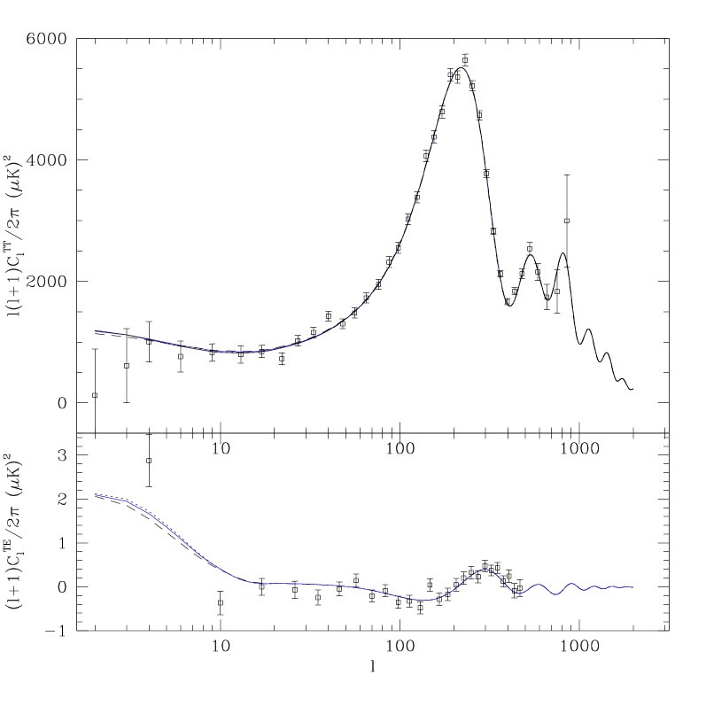
Figure 2: CMB temperature angular power spectrum (TT) and the temperature-polarization cross-correlation (TE) for the three models in Fig. 1 (using the same conventions for the three line types) with the WMAP’s first year data.

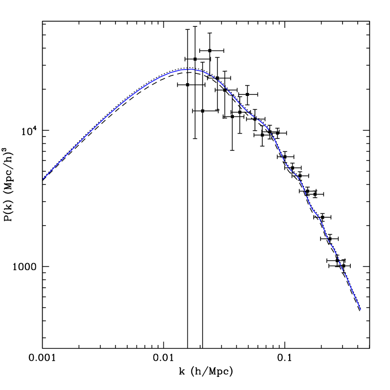
Figure 3: The linear matter power spectrum for the three models in Fig. 1. The SDSS data points sdss_pk are plotted to show current experimental error bars.

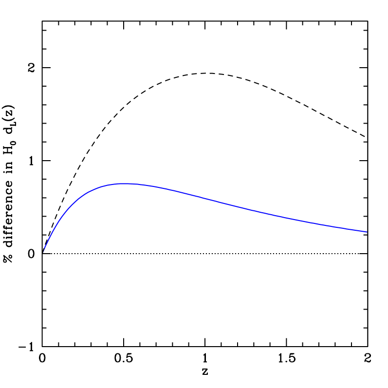
Figure 4: The percent difference in $H_{0}d_{L}(z)$ between the model with constant $w=-0.9$ (dotted line) and Models I (solid blue) and Model II (black dash). Current SNa data can determine $H_{0}d_{L}(z)$ with an accuracy of $5-10$%. Future data sets, such as supernovae from SNAP, can achieve an accuracy of $1-2$%.

Forecasts obtained using Fisher analysis are sensitive to the choice of the fiducial model. We will consider the same fiducial models for the two dark energy parameterizations discussed above and plotted in Fig. 1. The fiducial parameters for Model I were taken to be $w_{0}=-0.98$ and $\delta_{w}=-0.29$. For Model II we chose $\left<w\right>=-0.9$, $\Delta_{w}=-0.6$ and $\Delta_{z}=0.3$. We take all other cosmological parameters to be the same for both models. We have set the Hubble parameter $h=0.69$, baryon density $\Omega_{b}h^{2}=0.024$, total matter density $\Omega_{M}h^{2}=0.14$, spectral index $n_{s}=0.99$, optical depth $\tau=0.166$ and the amplitude of scalar fluctuations $A_{s}=0.86$ (as defined in wmap_verde .)

All of current data is consistent with $w={\rm const}=-0.9$ at $1\sigma$ level Spergel . Both, Model I and Model II, have the same weighted average $\left<w\right>=-0.9$. This assures that these two models have nearly identical CMB spectra as shown in Fig. 2.

In Fig. 3 we compare the matter power spectra predicted by the two models. Plotted are the linear CDM spectra at $z=0$. The bias, non-linear effects and the redshift space distortion would modify the three spectra in a similar way. While one cannot compare these linear spectra to the data without accounting for the above-mentioned corrections, we include the SDSS data points sdss_pk to illustrate the uncertainty in the current determination of $P(k)$.

Models I and II are also consistent with current estimates of the change in luminosity distance $d_{L}(z)$ obtained from the SNIa measurements. In Fig. 4 we plot the percent difference in $H_{0}d_{L}$ between the model with constant $w=-0.9$ and Models I and Model II. The differences between the models are of order $1-2$%, well below the current level uncertainty and comparable to the projected accuracy of SNAP.

Hence, present data cannot distinguish between $w={\rm const}=-0.9$ and our Models I and II and both are perfectly consistent with all available observations.

III Experiments

We are interested in forecasting the errors in dark energy parameters that can be extracted from CMB/LSS correlation studies and compare them to those expected from the luminosity distance measurements. We make short- (less than 5 years) and long- (ten years) term predictions based on the ongoing and planned CMB, galaxy and SNe observations.

For our short term predictions we assume the 4-year CMB temperature and polarization data from WMAP wmap , the expected galaxy counts from the Dark Energy Survey (DES) des , and the SNe from the Nearby Supernova Factory (NSNF) nsfactory and the Supernovae Legacy Survey (SNLS) snls . In addition, we impose a Gaussian prior on the value of $h$ corresponding to a $1\sigma$ uncertainty of $\pm 0.08$ from the Hubble Space Telescope’s Key Project (HSTKP) hconstraint .

For the long term predictions we assume the 14 months CMB temperature and polarization data by Planck satellite planck , the galaxy catalogues by the Large Synoptic Survey Telescope (LSST) lsst , and the SNe from the Supernovae Acceleration Probe (SNAP) snap complemented by those from the NSNF.

III.1 Galaxy data: DES and LSST

Figure 5: The galaxy number distribution vs. redshift expected from the DES survey.

Figure 6: The galaxy number distribution vs. redshift for the “conservative” LSST survey.

Figure 7: The galaxy number distribution vs. redshift for the “goal” LSST survey.

To describe the distribution of galaxies from a given survey, we take the total galaxy number density to have the following redshift dependence hu_scran :

$$n_{g}^{\mathrm{tot}}(z)\propto z^{2}e^{-(z/z_{n})^{2}},$$ (23)

where $z_{n}$ is a parameter that is adjusted to reproduce the expected median redshift of the survey. The galaxies are further divided into photometric redshift bins, i. e.

$$n_{g}^{\mathrm{tot}}(z)=\sum_{i}n_{g}^{i}(z).$$ (24)

Following reference hu_scran , we assume that the photometric redshift errors are Gaussian distributed, and that their rms fluctuations increase with redshift as $\sigma(z)=\sigma_{\mathrm{max}}(1+z)/(1+z_{\mathrm{max}})$. The bins sizes are chosen to increase proportionally to the errors. The resulting photometric redshift distributions are given by,

$$n_{g}^{i}(z)=\frac{1}{2}n_{g}^{\mathrm{tot}}(z)\left[\mathrm{erfc}\biggl{(}\frac{z_{i-1}-z}{\sqrt{2}\sigma(z)}\biggr{)}-\mathrm{erfc}\biggl{(}\frac{z_{i}-z}{\sqrt{2}\sigma(z)}\biggr{)}\right],$$ (25)

where erfc is the complementary error function.

For a given photometric redshift bin, the normalized selection function is given by

$$W_{g}^{i}(z)=\frac{n_{g}^{i}(z)}{\bar{N}^{i}}\,$$ (26)

where $\bar{N}^{i}$ is the total number of galaxies in the $i$-th bin. The Poisson noise is uncorrelated between bins and contributes only to the galaxy angular auto-correlation as

$$N^{(i,j)}_{\ell}=\frac{\delta_{ij}}{\bar{n}_{A}^{i}},$$ (27)

where $\delta_{ij}$ is the Kronecker delta and $\bar{n}_{A}^{i}$ is the galaxy number per solid angle in the $i$-th bin. The observed correlation $\tilde{\omega}^{(i,j)}_{\ell}$ is the sum of the signal and the Poisson noise:

$$\tilde{\omega}^{(i,j)}_{\ell}\equiv\omega^{(i,j)}_{\ell}+N^{(i,j)}_{\ell}\,$$ (28)

The Dark Energy Survey (DES) is designed to probe the redshift range $0.1<z<1.3$ with an approximate 1-$\sigma$ error of $0.1$ in photometric redshift. This roughly corresponds to four bins (see Fig. 5) and a median redshift of $z=0.6$. The total expected number of galaxies is approximately $250$ million in a $5000$ sq. deg. area on the sky, or $f_{sky}=0.13$.

The proposed LSST survey is expected to cover up to $20,000$ sq. deg. of the sky and catalogue over a billion galaxies out to $z\sim 3$. We consider two cases: the conservative scenario case with $f_{sky}=0.3$ and $7$ photometric redshift bins out to $z\sim 1.5$, and the desired case with $f_{sky}=0.5$ and $10$ photometric redshift bins out to $z\sim 3$. For both cases we assume $70$ gal$/$arcmin². The assumed galaxy number distributions for the two cases are shown in Figs. 6 and 7. In what follows, we will refer to the two LSST cases as “conservative” and “goal”.

The photometric redshift errors used in our analysis should be seen as the optimistic values for the respective experiments. For a discussion of potential sources of systematic errors in photo-z estimates the reader is referred to Huterer05 ; Ma05 .

III.2 CMB data: WMAP and Planck

The latest expected values for the sensitivity and the resolution parameters of the 4-year WMAP and 14 months Planck missions are available in wmap ; planck . To make comparison with previous results easier, we opted to use similar, although somewhat different, parameters employed in Rocha ; Khoury for the three highest frequency channels of WMAP and the lowest three Planck HFI channels. We have checked that using the exact parameters given in wmap ; planck would lead to an insignificant modification of our results. The relevant parameters are listed in Table 1.

Table 1: The relevant parameters of WMAP wmap and Planck planck . We use the three highest frequency WMAP channels and the lowest Planck HFI frequency channels.

	WMAP			Planck
$\nu$ (GHz)	41	61	94	100	143	217
$\theta_{\mathrm{FWHM}}$ (arc min)	28	21	13	10.7	8.0	5.5
$\sigma_{T}$ ($\mu$K)	22	29	49	5.4	6.0	13.1
$\sigma_{E}$ ($\mu$K)	30	45	75	n/a	11.4	26.7
$f_{\mathrm{sky}}$		0.8			0.8

The noise contribution to the CMB temperature auto-correlation (TT) and the E-mode polarization (EE) spectra from one frequency channel is given by

$$N_{\ell,c}^{AA}=\bigg{(}\frac{\sigma_{A,c}\ \theta_{\mathrm{FWHM},c}}{T_{\mathrm{CMB}}}\bigg{)}^{2}e^{\ell(\ell+1)\theta^{2}_{\mathrm{FWHM},c}/8\ln 2},$$

where $c$ labels the channel and $A=T,E$. The combined noise from all channels is

$$N_{\ell}^{AA}=\left[\sum_{c}(N_{\ell,c}^{AA})^{-1}\right]^{-1}\ .$$ (29)

The observed spectra, i.e. the signal plus the noise, are then

$$\tilde{C}^{AA}_{\ell}\equiv C^{AA}_{\ell}+N^{AA}_{\ell}.$$ (30)

III.3 SN data: SNLS and SNAP

Table 2: The redshift distribution of type Ia supernovae $N(z)$ for SNLS snls and SNAP kim_etal , together with 300 SNe from the NSNF. The redshifts given are the upper limits of each bin. Magnitude errors $\sigma_{m}(z)$ are evaluated at bin midpoints.

	$z\rightarrow$	0.1	0.2	0.3	0.4	0.5	0.6	0.7	0.8	0.9	1.0	1.1	1.2	1.3	1.4	1.5	1.6	1.7
SNLS	$N(z)$	300	56	70	84	133	105	84	84	42	7
	$\sigma_{m}(z)$ ($\times 10^{-3}$)	9	20	19	18	16	19	22	23	29	60
SNAP	$N(z)$	300	35	64	95	124	150	171	183	179	170	155	142	130	119	107	94	80
	$\sigma_{m}(z)$ ($\times 10^{-3}$)	9	25	19	16	14	14	14	14	15	16	17	18	20	21	22	23	26

The DE constraints from supernovae surveys depend on the depth of the survey, the total number of the supernovae and their redshift distribution, i. e. on the number of SNe per redshift bin. For example, when constraining an evolving equation of state, it is known frieman_etal that the choice of the distribution affects the bounds on the relevant parameters (e.g.  $[w_{0}$,$\delta_{w}$]).

SNe observations determine the magnitude, $m(z)$, defined in eq. (18). The uncertainty in $m(z)$, at any $z$-bin containing $N_{\mathrm{bin}}$ supernovae, is given by

$$\sigma_{m}(z)=\sqrt{\frac{\sigma_{\mathrm{obs}}^{2}}{N_{\mathrm{bin}}}+\mathrm{d}m^{2}},$$ (31)

and we assume $\sigma_{\mathrm{obs}}=0.15$. The systematic error, $\mathrm{d}m$, is assumed to increase linearly with redshift:

$$\mathrm{d}m=\delta m\frac{z}{z_{\mathrm{max}}},$$ (32)

$\delta m$ being the expected uncertainty and $z_{\mathrm{max}}$ the maximum redshift.

The SNLS is expected to measure approximately 700 supernovae out to $z_{\mathrm{max}}=1$ with an uncertainty $\delta m=0.02$. The SNLS supernovae distribution that we use for our short term forecasts is shown in Table 2. The ground-based NSNF experiment nsfactory will add to the count  300 SNe at $z\lesssim 0.1$.

SNAP will provide over 2000 supernovae with $\delta m=0.02$ and $z_{\mathrm{max}}=1.7$. In this work we have considered a fiducial SNAP survey analogous to the one modeled in kim_etal . The parameters are given in Table 2.

In addition to supernovae, SNAP can get over 300 million galaxies (at $n_{gal}=100$ arcmin^-2) at moderate and high redshifts, covering potentially up to $10,000$ sq.deg of the sky. This would make it a candidate survey for ISW studies .

IV Results and Discussion

IV.1 Cross correlations and $\mathbf{w(z)}$

As discussed earlier, CMB is sensitive primarily to a particular weighted average of the dark energy equation of state, given by $\left<w\right>$ huey99 ; dave02 ; saini03 . Measurements of the acceleration by SNe are predominantly sensitive to the very low redshift behavior of $w(z)$. The cross correlation measurements, on the other hand, can give an independent window on the behavior of the equation of state at intermediate redshifts. In this subsection we justify our expectation for the CMB/LSS cross-correlation to be an effective probe of $w(z)$. Additional analysis of the dependence of the cross correlation on the time evolution of the DE equation of state can be found in GPV04 ; Levon04 .

First note that in the small angle limit, the cross correlation can be written as

$$X(\theta\rightarrow 0)\approx{const}\int dz\ W_{g}(z)D(z){d\over dz}\left[(1+z)D(z)\right]\ .$$ (33)

where $D(z)\equiv\delta(k,z)/\delta(k,0)$ is the linear growth factor and we used the Poisson equation to express $\Phi$ in terms of $\delta$: $\Phi(k,z)\propto(1+z)\delta(k,z)$. The small angle limit $X(\theta\rightarrow 0)$ is representative of the total cross-correlation signal inside the redshift window $W_{g}(z)$ Levon04 .

Eq. (33) shows that the cross-correlation is essentially the product of the growth function and its derivative averaged over a given range of redshifts. Having several weakly overlapping selection functions $W_{g}^{i}(z)$, as in the case of LSST (e.g. see Fig. 7), would allow one to effectively map the evolution of this product. Since the rate of the growth is a particularly sensitive probe of the details of the dark energy evolution (see CHB03 for a discussion), cross-correlation studies can provide useful information despite large statistical errors.

Figure 8: The percent change in $P(z)$ (eq. (34), solid line), $d_{L}(z)$ (dot), $[D(z)]^{2}$ (dash) and $\Omega_{DE}(z)$ (dash-dot) caused by a $10$% change in $\Delta_{w}$, while holding $\left<w\right>$ fixed.

To illustrate the sensitivity of the cross-correlation to changes in the evolution of $w(z)$, we look at the change in the quantity

$$P(z)\equiv D(z){d\over dz}\left[(1+z)D(z)\right]$$ (34)

caused by a $10$% decrease in the parameter $\Delta_{w}$ of our Model II. We hold the other two DE parameters, $\left<w\right>$ and $\Delta_{z}$, as well as the cosmological parameters, fixed at their fiducial values. Then we compare the resulting relative difference in $P(z)$ to the differences in $[D(z)]^{2}$ and in $d_{L}(z)$. As one can see in Fig. 8, $P(z)$ is by far the more sensitive probe of the three. Also note, that the evolution of $P(z)$ is almost identically tracing the evolution of the DE fraction $\Omega_{DE}(z)$. This is expected, since the change in the gravitational potential $\Phi(z)$ is directly caused by a non-zero $\Omega_{DE}(z)$. In particular, it is shown in Wang98 that the evolution of $(1+z)D(z)$ couples to $w(z)\Omega_{DE}(z)$.

It is possible to explain the differences in Fig. 8 qualitatively. The reason $d_{L}(z)$ is not sensitive to a change in $\Delta_{w}$ is mainly due to the change occurring at a high redshift: $z_{T}\sim 1.2$. The main contribution to $d_{L}(z)$ in the integral given by eq. (19) comes from low redshifts, where $w(z)$ is not affected by a change in $\Delta_{w}$. That is, $w=-1$ at low redshifts for any small variation around Model II.

A change in $\Delta_{w}$ (while holding $\left<w\right>$ fixed) affects the observables via a combination of two effects. One is the change in the high redshift value of $w$, which alters the DE fraction at early times. The second is the change in the transition redshift, $z_{T}$. The change to the growth factor comes mainly from the first of the two effects, while $P(z)$ is affected by both.

The sensitivity of $P(z)$ to $w(z)$ is off-set by the large variance in cross-correlation measurements. Below we present results of the Fisher analysis that reflect this limitation.

IV.2 Bias

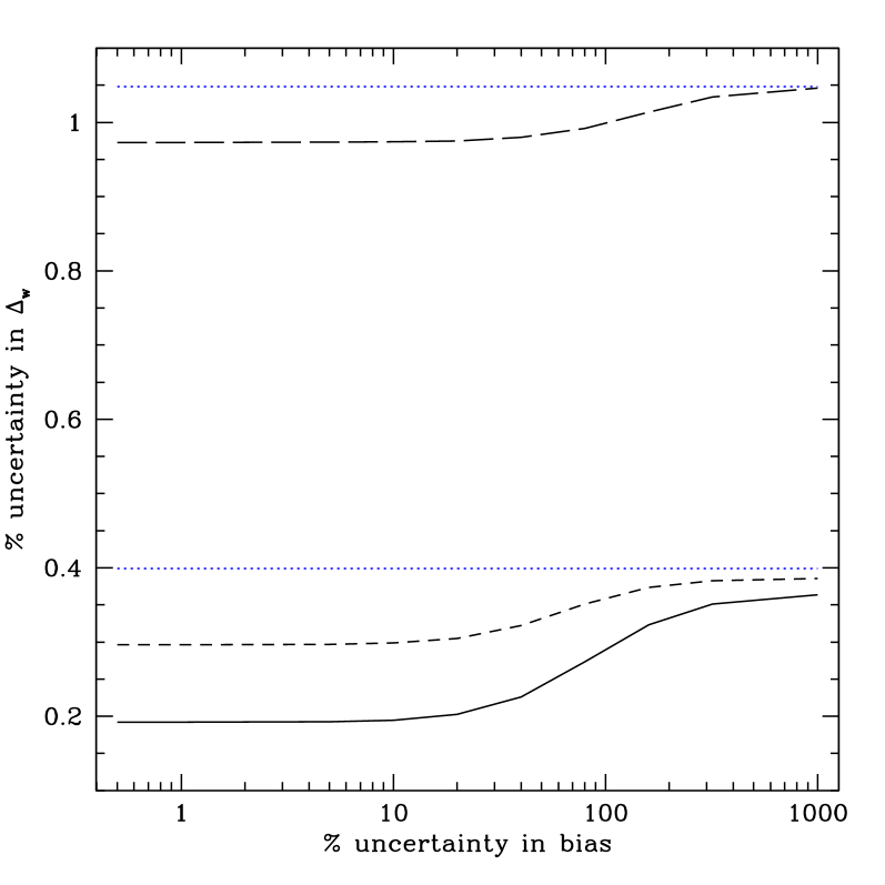
Figure 9: The dependence of the uncertainty in the Model II parameter $\Delta_{w}$ on the assumed bias prior. The long dash line corresponds to the error from the CMB/LSS cross-correlation using WMAP and DES, the short dash-line from Planck and the “conservative” LSST, and the solid line from Planck and the “goal” LSST. The blue dot lines are the expected errors in $\Delta_{w}$ from the WMAP data alone (the upper dotted line) and from Planck alone (the lower dotted line) shown for reference.

Most of the contribution to the CMB/LSS correlation signal comes from large scales , where perturbations are well described by the linear theory. On such scales, galaxies are expected to closely trace the distribution of dark matter, up to a scale-independent bias factor $b_{g}$. The bias is also known to vary with redshift, hence, each of the photometric bins will, in principle, have a different bias factor. The bias factors corresponding to each bin can be determined from the amplitude of the primordial spectrum extracted from the CMB and the galaxy-galaxy autocorrelation spectra. It is reasonable to assume that the bias in each bin can be determined with $10$% accuracy.

We account for the bias uncertainty by assigning an independent constant bias factor to each bin and treating them as parameters in our Fisher analysis. We assume that the value of the bias can be determined from elsewhere to a $10$% accuracy in all bins. This assumption, which we implement by imposing a prior, does not have a big influence on our final results, as long as the bias in each bin is known to better than $20$%. This is illustrated in Fig. 9, where we plot the predicted Fisher error in $\Delta_{w}$ as a function of the assumed uncertainty in bias. The fiducial values of the bias parameters were chosen to be the same for all bins. Choosing them according to a fixed function of redshift does not noticeably affect the results of the Fisher analysis.

IV.3 Short term prospects

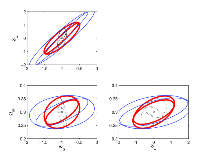
Figure 10: The expected $1\sigma$ projected contours for the $\Lambda$CDM fiducial model from WMAP (thin blue), and the information from WMAP combined with the WMAP/DES correlation (thick solid red) and SNLS supernovae (black dot), using the linear parameterization of eq. (1). For each line-type, the smaller ellipses correspond to including the CMB polarization information, while the larger ellipses are obtained using the CMB temperature spectra only. A prior from HSTKP on the value of $h$ is used.

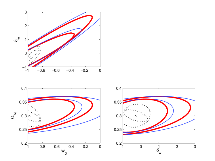
Figure 11: Short term forecasts of uncertainties on the parameters of Model I. Shown are the $1\sigma$ projected contours from WMAP (thin blue), and the WMAP information combined with the WMAP/DES correlation (thick solid red) and SNLS supernovae (black dot). As in Fig. 10, the smaller ellipses correspond to including the CMB polarization information, while the larger ellipses are obtained using the CMB temperature spectra only. A prior from HSTKP on the value of $h$ is used.

In the next few years we will have results from DES, SNLS and the complete data from WMAP, which will include E-mode polarization. In this subsection we show and compare the expected constraints on $w(z)$ from these measurements.

The linear parameterization of $w(z)$ (eq. (1)) with fiducial parameters corresponding to $\Lambda$CDM ($w_{0}=-1$, $\delta_{w}=0$) is the most commonly considered case in the existing literature. For that reason we include it in our analysis and show the short term prediction for the DE parameters in Fig. 10. Shown are only the contours for $\Omega_{M}$, $w_{0}$ and $\delta_{w}$, with other parameters being marginalized over. In this case, the cross-correlation information provides only a modest improvement over the CMB spectra alone. Supernovae data, on the other hand, can tighten the allowed range of the DE model parameters somewhat better and significantly constrain $w_{0}$.

Table 3: Short term predictions assuming WMAP for CMB, SNLS+NSNF for SNe and WMAP/DES for the CMB/LSS cross-correlation ($X$). The SNe and X results are shown with priors from CMB temperature only (T) and CMB temperature and polarization data combined (TP). A prior from HSTKP on the value of $h$ is used.

		Model I, $1\sigma$ errors						Model II, $1\sigma$ errors
		CMB		SNe		X		CMB		SNe		X
p	${\rm fiducial}\atop{\rm values}$	T	TP	T	TP	T	TP	T	TP	T	TP	T	TP
$w_{0}$	-0.98	1.1	0.73	0.16	0.15	0.87	0.62	-	-	-	-	-	-
$\delta_{w}$	-0.29	3.8	2.1	0.82	0.66	3.0	1.8	-	-	-	-	-	-
$\left<w\right>$	-0.9	-	-	-	-	-	-	0.26	0.19	0.22	0.13	0.23	0.17
$\Delta_{w}$	-0.6	-	-	-	-	-	-	3.2	1.0	2.9	1.0	2.0	0.97
$\Delta_{z}$	0.3	-	-	-	-	-	-	8.9	6.2	4.0	2.6	6.6	4.7
$\Omega_{M}$	0.3	0.07	0.06	0.04	0.02	0.07	0.06	0.07	0.06	0.05	0.03	0.07	0.05
$h$	0.69	0.07	0.07	0.03	0.02	0.07	0.07	0.08	0.07	0.06	0.04	0.07	0.06
$10^{3}\omega_{b}$	24	2	0.7	2	0.6	2	0.7	3.4	0.8	3.2	0.7	2.7	0.7
$n_{s}$	0.99	0.08	0.02	0.07	0.02	0.07	0.02	0.13	0.02	0.12	0.02	0.1	0.02
$\tau$	0.166	0.17	0.02	0.15	0.02	0.15	0.02	0.22	0.02	0.22	0.02	0.2	0.02
$A_{s}$	0.9	0.3	0.04	0.28	0.04	0.27	0.04	0.4	0.04	0.39	0.04	0.35	0.04

The short term predictions for Model I are shown in Fig. 11, again, for $\Omega_{M}$, $w_{0}$ and $\delta_{w}$ only. The list of predicted uncertainties in all parameters of Model I is given in Table 3. The expected uncertainties are different, and generally larger than in the $\Lambda$CDM fiducial case. This illustrates the importance of the underlying DE model for constraining $w(z)$. The cross-correlation will not, in short term, provide competitive constraints on the evolution of $w(z)$ according to $\Lambda$CDM or Model I.

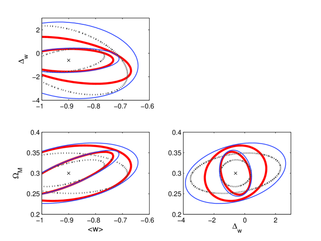
Figure 12: The expected $1\sigma$ projected contours from WMAP (thin blue), and the WMAP information combined with the WMAP/DES correlation (thick solid red) and SNLS supernovae (black dot) for Model II. The smaller ellipses correspond to including the CMB polarization information, while the larger ellipses are obtained from the CMB temperature spectra alone. A prior from HSTKP on the value of $h$ is used.

The forecasts for Model II parameters $\left<w\right>$, $\Delta_{w}$ and $\Omega_{M}$ are shown in Fig. 12, while Table 3 contains the full list of the expected parameter uncertainties. The choice of the model clearly makes a big difference. Most notably, neither the short term SNe nor the cross-correlation measurements can improve the CMB bounds on $\Delta_{w}$. The SNe, on the other hand, are still useful in tightening the constraint on $\Omega_{M}$ and $\left<w\right>$. Overall, it is clear from the plots and the table that measurements of the cross-correlation in the next five years will not provide any new competitive constraint on the evolution of $w$. In the case of Model II this is primarily due to limited depth of the DES survey, which does not sample the redshifts above $z\sim 1$, where the transition in $w(z)$ occurs. In the case of Model I, constraints from the cross-correlation are even weaker, even though it has one less parameter as compared to Model II. It is worth noticing that for this model, the degeneracy between $w_{0}$ and $\delta_{w}$ that hinders their determination from CMB alone (with a prior on $h$) is slightly improved by the addition of the cross-correlation information. This is because the angular diameter distance to last scattering surface depends on the dark energy through the average equation of state value $\left<w\right>$. Therefore in Model I different values of $w_{0}$ and $\delta_{w}$ can give the same $\left<w\right>$. On the other hand redshift dependent measurements of the ISW-correlation are sensitive to both the average equation of state and its time evolution improving the constraints on these two parameters.

In summary, the short term cross-correlation measurements will not be competitive, while supernovae measurements will only constrain $w_{0}$ of Model I and $\left<w\right>$ of Model II. As we will see in the next subsection, the constraints on all parameters tighten in the case of deeper surveys such as LSST.

IV.4 Long term prospects

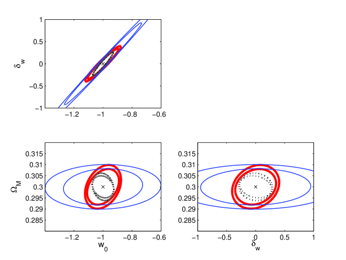
Figure 13: The expected $1\sigma$ projected contours from Planck (thin blue), and Planck information combined with the Planck/LSST(goal) correlation (thick solid red) and SNAP supernovae (black dot) for the linear parameterization of eq. (1) with $\Lambda$CDM fiducial parameters. (Compare this to Fig. 10).

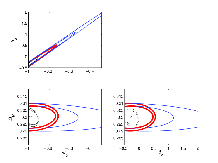
Figure 14: The expected $1\sigma$ projected contours for the Model I parameters from Planck (thin blue), and Planck information combined with the Planck/LSST(goal) correlation (thick solid red) and SNAP supernovae (black dot). (Compare this to Fig. 11).

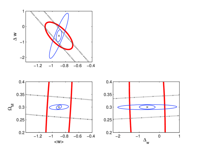
Figure 15: The expected $1\sigma$ projected contours for the Model II parameters from the three probes: Planck (thin blue), Planck/LSST(goal) correlation (thick solid red) and SNAP supernovae (black dot).

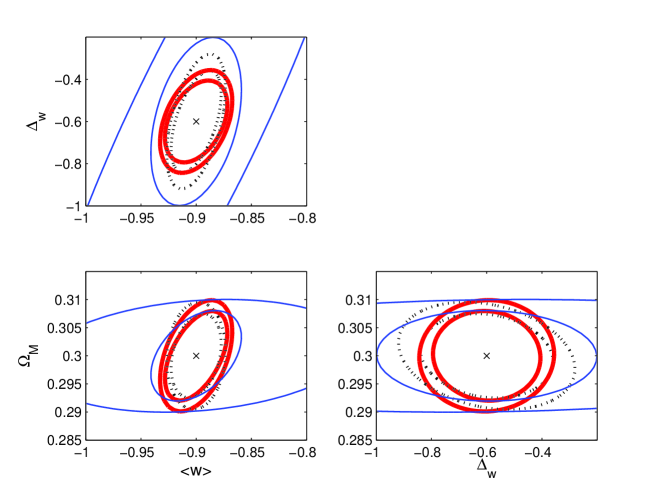
Figure 16: The expected $1\sigma$ projected contours for the Model II parameters from Planck (thin blue), and Planck information combined with the Planck/LSST(goal) correlation (thick solid red) and SNAP supernovae (black dot). (Compare this to Fig. 12).

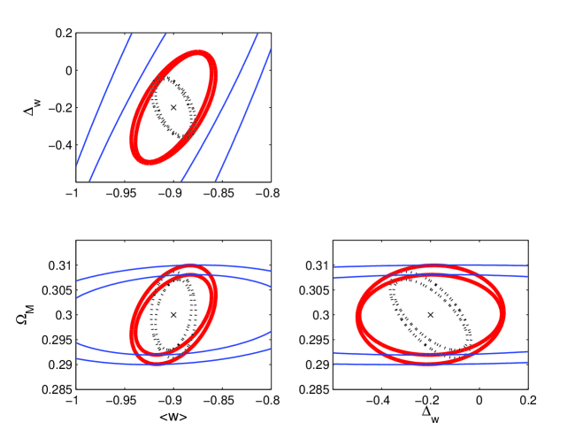
Figure 17: Same as Fig. 16 but using a fiducial $\Delta_{w}=-0.2$.

Table 4: Long term predictions assuming Planck for CMB, SNAP+NSNF for SNe and Planck/LSST for the CMB/LSS cross-correlation ($X$) for the“conservative” and “goal” cases. The SNe and $X$ results are shown with priors from CMB temperature only (T) and CMB temperature and polarization data combined (TP).

		Model I, $1\sigma$ errors								Model II, $1\sigma$ errors
		CMB		SNe		X(conserv.)		X(goal)		CMB		SNe		X(conserv.)		X(goal)
p	${\rm fiducial}\atop{\rm values}$	T	TP	T	TP	T	TP	T	TP	T	TP	T	TP	T	TP	T	TP
$w_{0}$	-0.98	0.86	0.46	0.08	0.08	0.41	0.33	0.26	0.24	-	-	-	-	-	-	-	-
$\delta_{w}$	-0.29	2.8	1.5	0.28	0.27	1.3	1.0	0.84	0.76	-	-	-	-	-	-	-	-
$\left<w\right>$	-0.9	-	-	-	-	-	-	-	-	0.14	0.04	0.03	0.02	0.04	0.03	0.03	0.03
$\Delta_{w}$	-0.6	-	-	-	-	-	-	-	-	1.5	0.39	0.32	0.24	0.44	0.3	0.24	0.19
$\Delta_{z}$	0.3	-	-	-	-	-	-	-	-	8.3	4.5	0.9	0.79	2.4	2.2	1.3	1.2
$\Omega_{M}$	0.3	0.01	0.008	0.007	0.005	0.01	0.008	0.01	0.008	0.01	0.008	0.009	0.007	0.01	0.008	0.01	0.008
$h$	0.69	0.01	0.009	0.006	0.005	0.01	0.009	0.01	0.009	0.01	0.009	0.01	0.008	0.01	0.009	0.01	0.009
$10^{3}\omega_{b}$	24	0.21	0.16	0.2	0.16	0.21	0.16	0.21	0.16	0.22	0.16	0.2	0.16	0.21	0.16	0.21	0.16
$n_{s}$	0.99	0.005	0.004	0.005	0.004	0.005	0.004	0.005	0.004	0.005	0.004	0.005	0.004	0.005	0.004	0.005	0.004
$\tau$	0.166	0.04	0.006	0.03	0.005	0.03	0.006	0.03	0.006	0.05	0.007	0.03	0.006	0.03	0.006	0.03	0.006
$A_{s}$	0.9	0.07	0.01	0.06	0.01	0.06	0.01	0.06	0.01	0.1	0.01	0.06	0.01	0.06	0.01	0.06	0.01

In the longer term, i.e. in the next ten years, we should expect to have the results from Planck CMB measurements, galaxy catalogues from LSST and the SNe measurements from SNAP. These will significantly improve the constraints on the DE parameters. In certain models, as we show here on the example of our Model II, CMB/LSS cross-correlation can play a competitive role.

As in the previous subsection, we begin by considering the linear DE model with two different sets of the fiducial values: one where they match a cosmological constant ($w_{0}=-1,\delta_{w}=0$) and another where $w$ evolves but still consistent with present observations (Model I). In Fig. 13 and Fig. 14 we show the $1\sigma$ projected contours for the linear models. On these plots, the cross-correlation and the SNe prediction includes the information from Planck. Combining with Planck is equivalent to applying strong priors on all cosmological parameters. The constraints in the absence of any priors can be found in Table 4. Planck and SNAP are by far the most dominant information sources for these models, with cross-correlation adding a relatively weak contribution.

For Model II we start by presenting the individual error contours for the three experiments (Fig. 15), with the purpose of explicitely showing degeneracy directions. We will see that, once we consider its combination with Planck, the

relative utility of the cross-correlation is significantly higher for Model II. The contours in Fig. 16 show that the cross-correlation can provide constraints on $\left<w\right>$ and $\Delta_{w}$ that are competitive with those from SNAP. The improvement on Planck is especially strong without the polarization data. The full list of parameter constraints is given in Table 4. Our results confirm that SNe measurements are more suitable for constraining variations in $w(z)$ at low redshifts. At higher redshifts, the cross-correlation becomes useful and can provide an independent constraint $\Delta_{w}$.

Figure 17 illustrates how a different choice of Model II fiducial parameters affects the constraining capabilities of the different probes. The alternative model has $\Delta_{w}=-0.2$ instead of $-0.6$ . In this case we note the SNAP+Planck constraint for $\Delta_{w}$ is noticeably tighter than that from the Planck/LSST correlation. Also note that this is mainly due to improvement in the sensitivity of the SNe, as the transition in this model happens at a lower redshfit. The size of the error on $\Delta_{w}$ from the cross-correlation is only marginally increased compared to Fig. 16.

V Conclusions

We have studied the potential of the CMB/LSS correlation for constraining the evolution of the DE equation of state. We proposed a new parameterization, a “Kink” model which has the average equation of state $\left<w\right>$ as an explicit parameter. A direct control on the value of $\left<w\right>$ preserves the tight constraints on $w$ obtained from the distance to last scattering measurements, while allowing $w(z)$ to vary in other ways.

Using Fisher analysis, we have made forecasts of the expected uncertainties in DE parameters extracted from the upcoming CMB, SNe and CMB/LSS correlation data. We have considered both short- (WMAP, DES, SNLS) and long- (Planck, LSST, SNAP) term prospects. We find that in long term the cross-correlation will provide competitive constraints on the evolution of $w(z)$, in particular, on the total change in $w$, provided a sufficiently generic parameterization is used. We also note that the transition length parameter, $\Delta_{z}$, will not be well constrained even with the long-term combined data.

Our results encourage further investigation of the CMB/LSS correlation as a probe of dark energy. The cross-correlation has a clear weakness – a large variance that hinders its utility as a precision cosmology probe. However, it also has certain attractive features, that in some cases can out weigh the lack of accuracy. These features are:

• The cross-correlation probes the rate of the growth of structure as well as the growth.

• It is practically independent of reionization details ($\tau$) and the details of the initial spectrum ($n_{s}$).

• It probes the large scales ($0.01<k<0.1h{\rm Mpc}^{-1}$), where the evolution of structure is safely inside the linear regime and there is no need for higher order corrections.

• On linear scales contributing to the ISW/LSS correlation the galaxy bias is expected to be independent of scale.

• Cross-correlation is linear in bias, compared to the matter power spectrum that is quadratic. In fact, if one used a cross-correlation estimator that is normalized to the auto-correlations, that estimator would be independent of bias and the overall normalization of the primordial spectrum.

• Cross-correlation can probe the evolution of dark energy at relatively high redshifts, inaccessible by luminosity distance measurements.

In this work we have restricted our attention to Quintessence models for which the effective sound speed is of order of unity, so that the dark energy perturbations only affect the evolution of the largest structures. However, if the dark energy clusters on smaller scales, it may leave a distinctive signature which can be detected with cross-correlation measurements. Although current data do not provide any constraints on the dark energy sound speed bean03 ; CGM , the constraints from the next generation of galaxy surveys have been studied in hu_scran .

We have only considered flat FRW models. Without the flatness assumption, CMB constraints on $\Omega_{M}$ and $h$ weaken because of a well-known degeneracy BondEfstathiou , also relaxing constraints on $w(z)$. We will explore constraints on DE using ISW without the flatness prior in a future work.

The Model II type parameterization of $w(z)$ considered in the paper is not necessarily the most optimal for underscoring the power of cross-correlation constraints (although clearly better suited for this purposed than Model I). A more comprehensive study using a principal component approach HutererStarkman ; Crittenden05 is a subject of ongoing research.

Another potential use of the ISW cross-correlation is to measure the amplitude of the scalar perturbations and indirectly constrain the amplitude of the tensor modes when combined with the normalization of CMB spectra CCGM . This is because the distribution of the large scale structures is not correlated with a stochastic background of gravitational waves. It has been also suggested glenn that CMB/LSS studies may help to differentiate between Quintessence and models with modified gravity.

For a fixed total number of galaxies the information extracted from the ISW studies depends on the choice of the redshift binning. The role of cross-correlation in constraining $w(z)$ may be further increased by optimizing the bin selection. Such an optimization is a topic of ongoing research.

- (1) D. Spergel et al.(WMAP team), Astrophys. J. Suppl. 148, 175 (2003).
- (2) W. J. Percival et al., Mont. Not. R. Astron. Soc. 327, 1297 (2001); M. Tegmark et al., Astrophys. J. 606, 70 (2004).
- (3) A. Riess et al., Astron. J. 116, 1009 (1998); S. Perlmutter et al., Astrophys. J. 517, 565 (1999).
- (4) S. Boughn and R. Crittenden, astro-ph/0305001; Nature 427, 45 (2004).
- (5) M. R. Nolta et al., Astrophys. J. 608, 10 (2004), astro-ph/0305097.
- (6) P. Fosalba, E. Gaztanaga, MNRAS 350, L37 (2004), astro-ph/0305468; P. Fosalba, E. Gaztanaga, and F. Castander, Astrophys. J. Lett. 597, L89 (2003), astro-ph/0307249.
- (7) R. Scranton et al, astro-ph/0307335.
- (8) N. Afshordi, Y. S. Loh and M. A. Strauss, Phys. Rev. D69, 083524 (2004) astro-ph/0308260.
- (9) R. Sachs and A. Wolfe, Astrophys. J. 147, 73 (1967).
- (10) R. G. Crittenden and N. Turok, Phys. Rev. Lett. 76, 575 (1996).
- (11) Y.B. Zel’dovic and R.A. Sunyaev, Astrophys. Space Sci. 4, 301 (1969).
- (12) H. Peiris and D. Spergel, Astrophys. J. 540, 605 (2000).
- (13) A. D. Linde, Rept. Prog. Phys. 47, 925 (1984); A. Vilenkin, Phys. Rev. Lett. 74, 846 (1985); G. Efstathiou, MNRAS 274, L73 (1995); S. Weinberg, Phys. Rev. Lett. 59, 2607 (1987); H. Martel, P. R. Shapiro and S. Weinberg, Astrophys. J. 492, 29 (1998); J. Garriga, M. Livio and A. Vilenkin, Phys. Rev. D61, 023503 (2000); S. A. Bludman, Nucl. Phys. A663, 865 (2000); J. Garriga and A. Vilenkin, Phys. Rev. D67, 043503 (2003); L. Pogosian, A. Vilenkin, M. Tegmark, astro-ph/0404497, JCAP 0407 (2004) 005
- (14) M. Reuter, C. Wetterich, Phys. Lett. B188, 38 (1987).
- (15) B. Ratra and P. J. E. Peebles, Phys. Rev. D37, 3406 (1988).
- (16) R. R. Caldwell, R. Dave, Paul J. Steinhardt, Phys. Rev. Lett. 80, 1582 (1998).
- (17) Y. Wang and M. Tegmark, Phys. Rev. Lett. 92, 241302 (2004).
- (18) P.S. Corasaniti, M. Kunz, D. Parkinson, E.J. Copeland and B.A. Bassett, Phys. Rev. D70, 083006 (2004).
- (19) S. Hannestad and E. Mortsell, J. Cosmol. Astropar. Phys. 0409, 001 (2004).
- (20) B.A. Bassett, P.S. Corasaniti and M. Kunz, Astrophys. J. 617, L1 (2004).
- (21) D. Rapetti, S.W. Allen and J. Weller, astro-ph/0409574.
- (22) H. K. Jassal, J. S. Bagla, T. Padmanabhan, MNRAS Lett., 356, L11-L16, (2005).
- (23) J. Garriga, L. Pogosian and T. Vachaspati, Phys. Rev. D69, 063511 (2004), astro-ph/0311412.
- (24) L. Pogosian, JCAP 04, 015 (2005), astro-ph/0409059.
- (25) I. Maor, R. Brustein, J. McMahon and P.J. Steinhardt, Phys. Rev. D65, 123003 (2002).
- (26) J.M. Virey et al., Phys. Rev. D70, 121301 (2004).
- (27) M. Chevallier and D. Polarski, Int. J. Mod. Phys. D10, 213 (2001); E.V. Linder, Phys. Rev. Lett. 90, 91301 (2003).
- (28) A. Upadhye, M. Ishak and P. J. Steinhardt, astro-ph/0411803; E V. Linder and D. Huterer, astro-ph/0505330.
- (29) B. A. Bassett, M. Kunz, J. Silk and C. Ungarelli, Phys. Rev. D68, 043504 (2003).
- (30) P. S. Corasaniti, E. J. Copeland, Phys. Rev. D67 (2003) 063521.
- (31) G. Huey, L. Wang, R. Dave, R. R. Caldwell, P. J. Steinhardt, Phys. Rev. D59, 063005 (1999).
- (32) R. Dave, R. R. Caldwell, P. J. Steinhardt, Phys. Rev. D66, 023516 (2002).
- (33) T. D. Saini, T. Padmanabhan and S. Bridle, MNRAS 343, 533 (2003).
- (34) A. D. Linde, in 300 Years of Gravitation, ed. by S. W Hawking and W. Israel, Cambridge University Press (1987).
- (35) J. Garriga and A. Vilenkin, Phys. Rev. D61 (2000) 083502
- (36) A. Albrecht and C. Skordis, Phys. Rev. D64, 023514 (2001), astro-ph/9908085; T. Barreiro, E.J. Copeland and N.J. Nunes, Phys. Rev. D61, 127301 (2000), astro-ph/9910214; E.J. Copeland, N.J. Nunes and F. Rosati, Phys. Rev. D62, 123503 (2000), hep-ph/0005222.
- (37) M. Zaldariaga and U. Seljak, Astrophys. J. 469, 437 (1996); http://www.cmbfast.org
- (38) M. Tegmark, A. N. Taylor and A. F. Heavens, Astrophys. J. 480, 22 (1997).
- (39) M. Zaldarriaga and U. Seljak, Phys. Rev. D55, 1830 (1997).
- (40) L. Verde et al (WMAP collaboration), Astrophys. J. Suppl. 148, 195 (2003).
- (41) M. Tegmark et al (SDSS collaboration), Ap. J. 606, 702 (2004).
- (42) N. Jarosik et al, Astrophys. J. Suppl. 148, 29 (2003); http://map.gsfc.nasa.gov/
- (43) http://www.darkenergysurvey.org/
- (44) W.M. Wood-Vasey et al, New Astron. Rev. 48, 637 (2004).
- (45) http://cfht.hawaii.edu/SNLS/
- (46) W. L. Freedman et al (HST Key Project), Astrophys. J. 553, 47 (2001)
- (47) http://www.rssd.esa.int/SA/PLANCK/docs/goal-perf-sum-feb-2004.pdf
- (48) http://www.lsst.org/
- (49) http://snap.lbl.gov/
- (50) W. Hu and R. Scranton, Phys. Rev. D70 123002 (2004).
- (51) D. Huterer et al, astro-ph/0506030.
- (52) Z. Ma, W. Hu and D. Huterer, astro-ph/0506614, accepted to Ap.J.
- (53) G. Rocha et al., MNRAS, 352, 20 (2004).
- (54) S. Wang et al., Phys.Rev. D70, 123008 (2004).
- (55) J.A. Frieman, D. Huterer, E.V. Linder and M.S. Turner, Phys. Rev. D67, 083505 (2003).
- (56) A. G. Kim, E. V. Linder, R. Miquel and N. Mostek, Mon. Not. Astron.Soc. 347 909-920 (2004).
- (57) A. Cooray, D. Huterer and D. Baumann, Phys.Rev. D69 (2004) 027301, astro-ph/0304268.
- (58) L. Wang, P. J. Steinhardt, Astrophys.J. 508 (1998) 483-490, astro-ph/9804015.
- (59) R. Bean and O. Dore, Phys.Rev. D69, 083503 (2004), astro-ph/0307100.
- (60) P.S. Corasaniti, T. Giannantoni and A. Melchiorri, astro-ph/0504115.
- (61) J. R. Bond and G. Efstathiou, MNRAS, 304, 75 (1999).
- (62) D. Huterer and G. Starkman, Phys. Rev. Lett. 90, 031301 (2003).
- (63) R. G. Crittenden and L. Pogosian, astro-ph/0510293.
- (64) A. Cooray, P.S. Corasaniti, T. Giannantonio and A. Melchiorri, astro-ph/0504290.
- (65) A. Lue, R. Scoccimarro, G. Starkman, Phys.Rev. D69 (2004) 044005