Hot Neutron and Quark Star Evolution

Abstract

The physics of compact objects is one of the very actively developing branches of theoretical investigations, since the careful analysis of different models for the internal structure of these objects, their evolutionary characteristics and the comparison with modern observational data give access to discriminate among various speculations about the state of matter under extreme conditions.

The lecture provides an overview to the problem of neutron star cooling evolution. We discuss the scheme and necessary inputs for neutron star cooling simulations from the background of a microscopic modeling in order to present the surface temperature - age characteristics of hybrid neutron stars including the determination of main regulators of the cooling process, the question of neutrino production and diffusion.

1 Introduction

The interiors of compact stars are considered as systems where high-density phases of strongly interacting matter do occur in nature, see Shapiro and Teukolsky [1], Glendenning [2] and Weber [3] for textbooks. The consequences of different phase transition scenarios for the cooling behaviour of compact stars have been reviewed recently in comparison with existing X-ray data [4].

The Einstein Observatory was the first that started the experimental study of surface temperatures of isolated neutron stars (NS). Upper limits for some sources have been found. Then ROSAT offered first detections of surface temperatures. Next $X$-ray data came from Chandra and XMM/Newton. Appropriate references to the modern data can be found in recent works by [5, 6, 7, 8], devoted to the analysis of the new data. More upper limits and detections are expected from satellites planned to be sent in the nearest future. In general, the data can be separated in three groups. Some data show very “slow cooling” of objects, other demonstrate an “intermediate cooling” and some show very “rapid cooling”. Now we are at the position to carefully compare the data with existing cooling calculations.

The “standard” scenario of neutron star cooling is based on the main process responsible for the cooling, which is the modified Urca process (MU) $nn\rightarrow npe\bar{\nu}$ calculated using the free one pion exchange between nucleons, see [9]. However, this scenario explains only the group of slow cooling data. To explain a group of rapid cooling data “standard” scenario was supplemented by one of the so called “exotic” processes either with pion condensate, or with kaon condensate, or with hyperons, or involving the direct Urca (DU) reactions, see [10, 1] and refs therein. All these processes may occur only for the density higher than a critical density, $(2\div 6)~{}n_{0}$, depending on the model, where $n_{0}$ is the nuclear saturation density. An other alternative to ”exotic” processes is the DU process on quarks related to the phase transition to quark matter.

Particularly the studies of cooling evolution of compact objects can give an opportunity for understanding of properties of cold quark gluon plasma. In dense quark matter at temperatures below $\sim 50$ MeV, due to attractive interaction channels, the Cooper pairing instability is expected to occur which should lead to a variety of possible quark pair condensates corresponding to color superconductivity (CSC) phases, see [11] for a review.

Since it is difficult to provide low enough temperatures for CSC phases in heavy-ion collisions, only precursor phenomena [12, 13] are expected under these conditions.

CSC phases may occur in neutron star interiors [14] and could manifest themselves, e.g., in the cooling behavior [15, 16, 17, 18].

However, the domain of the QCD phase diagram where neutron star conditions are met is not yet accessible to Lattice QCD studies and theoretical approaches have to rely on non-perturbative QCD modeling. The class of models closest to QCD are Dyson-Schwinger equation (DSE) approaches which have been extended recently to finite temperatures and densities [19]. Within simple, infrared-dominant DSE models early studies of quark stars [20] and diquark condensation [21] have been performed.

Estimates of the cooling evolution have been performed [15] for a self-bound isothermal quark core neutron star (QCNS) which has a crust but no hadron shell, and for a quark star (QS) which has neither crust nor hadron shell. It has been shown there in the case of the 2SC (3SC) phase of QCNS that the consequences of the occurrence of gaps for the cooling curves are similar to the case of usual hadronic neutron stars (enhanced cooling). However, for the CFL case it has been shown that the cooling is extremely fast since the drop in the specific heat of superconducting quark matter dominates over the reduction of the neutrino emissivity. As has been pointed out there, the abnormal rate of the temperature drop is the consequence of the approximation of homogeneous temperature profiles the applicability of which should be limited by the heat transport effects. Page et al. (2000)[16] estimated the cooling of hybrid neutron stars (HNS) where heat transport effects within the superconducting quark core have been disregarded. Neutrino mean free path in color superconducting quark matter have been discussed in [22] where a short period of cooling delay at the onset of color superconductivity for a QS has been conjectured in accordance with the estimates of [15] in the CFL case for small gaps.

A completely new situation might arise if the scenarios suggested for (color) superconductivity [23, 24] besides of bigger pairing gaps ($\Delta_{q}\sim 50\div 100$ MeV) will allow also small diquark pairing gaps ($\Delta_{q}<1$ MeV) in quark matter.

The questions which should be considered within these models are the following: (i) Is strange quark matter relevant for structure and evolution of compact stars? (ii) Are stable hybrid stars with quark matter interior possible? (iii) What can we learn about possible CSC phases from neutron star cooling? Further on in this lectures we discuss the scheme and the results of realization of the these points in relation with the cooling evolution of compact objects.

In the consideration of the scenario for the thermal evolution of NS and HNS we include the heat transport in both the quark and the hadronic matter. We will demonstrate the influence of the diquark pairing gaps and the hadronic gaps on the evolution of the surface temperature.

The main strategy of the simulation of the cooling evolution of compact objects is presented in Fig 1. On the top of scheme we have the general theoretical background of QCD models as it has been discussed in the introduction. On the second level of the scheme we separate two branches one for the structure of the compact objects and the other for the thermal properties of the stellar matter. On the bottom of the scheme those two branches are combined in the code of the cooling simulations project and entail the comparison of the theoretical and observational results.

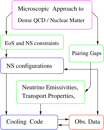
Figure 1: The scheme linked problems and tasks, which has to be done to simulate the cooling of compact objects

2 EoS of stellar matter and Compact Star configurations

2.1 Hadronic matter EoS and DU threshold

For the modeling of the dense hadronic matter different approaches, like relativistic and non-relativistic Brückner-Hartree-Fock approach including the three body correlations [25, 26, 27, 28] and different parameterizations of relativistic mean field models, are discussed successfully in the literature [29, 30, 31, 32].

For the appropriate cooling simulations we exploit the EoS of [25] (specifically the Argonne $V18+\delta v+UIX^{*}$ model), which is based on the most recent models for the nucleon-nucleon interaction including a parameterized three-body force and relativistic boost corrections. Actually we adopt a simple analytic parameterization of this model by Heiselberg and Hjorth-Jensen [28], hereafter HHJ.

The latter uses the compressional part with the compressibility $K\simeq 240$ MeV, a symmetry energy fitted to the data around nuclear saturation density and smoothly incorporates causality at high densities. The density dependence of the symmetry energy is very important since it determines the value of the threshold density for the DU process. The HHJ EoS fits the symmetry energy to the original Argonne $V18+\delta v+UIX^{*}$ model yielding $n_{c}^{\rm DU}\simeq~{}5.0~{}n_{0}$ ($M_{c}^{\rm DU}\simeq 1.839~{}M_{\odot}$).

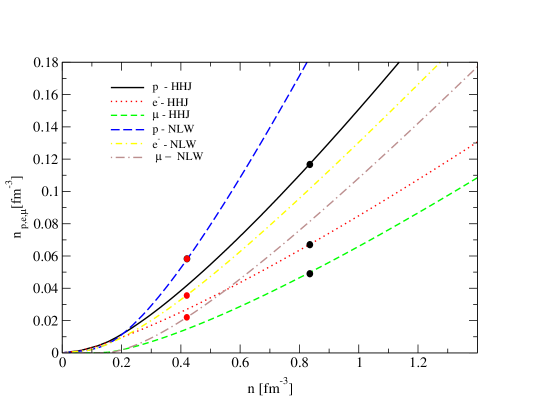
Figure 2: Densities of the charged particles as a function of baryon density for HHJ and NLW model EoS. Possibility of pion condensation is suppressed.

Fig. 2 demonstrates the partial densities of $p$, $e$ and $\mu^{-}$ in HHJ and relativistic non-linear Walecka (NLW) model in the parameterization of [32], adjusted to the following bulk parameters of the nuclear matter at saturation: $n_{0}=0.16$ fm^-3. Anyhow, in the given NLW model the threshold density for the DU process is $n_{c}^{\rm DU}\simeq~{}2.7~{}n_{0}$.

2.2 Quark matter EoS with 2SC superconductivity

The quark matter models [24, 33, 34] predict, that the diquark pairing condensate is possible for temperatures and densities relevant for compact objects. The order of magnitude of pairing gaps is 100 MeV and a remarkably rich phase structure of the matter has been identified [11, 35, 36, 37].

This leads to expectations of observable effects of color superconducting phases, particularly in the compact star cooling behaviour [15, 16, 17, 18, 38]. Generally color superconductivity is involved in all aspects of neutron star studies, such as magnetic field evolution [39, 40, 41, 42] or burst-type phenomena [43, 44, 45, 46].

The applications of the nonlocal chiral quark model developed in [47] for the case of neutron star constraints shows that the relevant CSC phase is a 2SC phase while the omission of the strange quark flavor is justified by the fact that chemical potentials in central parts of the stars do barely reach the threshold value at which the mass gap for strange quarks breaks down and they appear in the system [48, 49].

It has been shown in that work that the Gaussian formfactor ansatz of quark interaction (hereafter we call it SM model) leads to an early onset of the deconfinement transition and such a model is therefore suitable to discuss hybrid stars with large quark matter cores [50].

The resulting quark matter EoS within this nonlocal chiral model [47] can be represented in a form reminiscent of a bag model

$$P^{(s)}=P_{id}(\mu_{B})-B^{(s)}(\mu_{B})~{},$$ (1)

where $P_{id}(\mu_{B})$ is the ideal gas pressure of quarks and $B^{(s)}(\mu_{B})$ a density dependent bag pressure, see Fig. 3. The occurrence of diquark condensation depends on the value of the ratio $\eta=G_{2}/G_{1}$ of coupling constants and the superscript $s\in\{S,N\}$ indicating whether we consider the matter in the superconducting mixed phase ($\eta=1$) or in the normal phase ($\eta=0$), respectively.

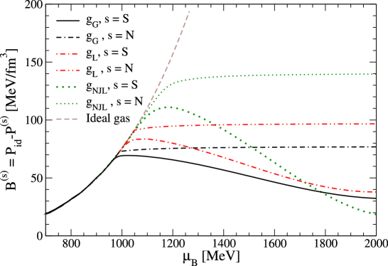
Figure 3: Bag pressure for different formfactors of the quark interaction in dependence on the baryon chemical potential for $\eta=0$ and for $\eta=1$. For the latter the superconducting phase is realized.

2.3 EoS of hybrid star matter

In some density interval above the onset of the first order phase transition, there may appear a mixed phase region between the hadronic (confined quark phase) and deconfined quark phases, see [51]. Ref. [51] disregarded finite size effects, such as surface tension and charge screening. On the example of the hadron-quark mixed phase Refs [52] demonstrated that finite size effects might play a crucial role substantially narrowing the region of the mixed phase or even forbidding its appearance in a hybrid star configuration. Therefore we omit the possibility of the hadron-quark mixed phase in our model assuming that the quark phase arises by the Maxwell construction.

To demonstrate the EoS with quark-hadron phase transition applicable for hybrid star configurations in the next Section, we show in Fig. 4 results using the relativistic mean field (RMF) model of asymmetric nuclear matter including a non-linear scalar field potential and the $\rho$ meson (nonlinear Walecka model) ( see [2]) for the cases $\eta=1$ (left panel) when the quark matter phase is superconducting and for $\eta=0$ (right panel) when it is normal.

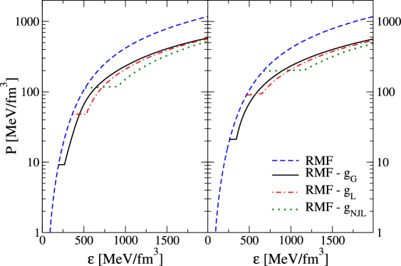
Figure 4: EoS for strongly interacting matter at zero temperature under compact star constraints for the coupling parameter $\eta=1$ (left panel) and $\eta=0$ (right panel). Dashed line: relativistic mean-field model for hadronic matter; solid, dash-dotted and dotted lines correspond to quark matter with Gaussian, Lorentzian and NJL formfactor functions, respectively.

In case the hadonic EoS is chosen to be HHJ model and the quark one is SM model we found a tiny density jump at the phase-boundary from $n_{c}^{\rm hadr}\simeq 0.44~{}{\rm fm}^{-3}$ to $n_{c}^{\rm quark}\simeq 0.46~{}{\rm fm}^{-3}$. The critical mass, when the branch of stable hybrid stars starts is $M_{c}^{\rm quark}=1.214~{}M_{\odot}$.

As shown in Refs. [53, 49] quark matter itself can exist in a mixed phase of 2SC and normal states. The presence or absence of the 2SC - normal quark mixed phase instead of only one of those phases is not so important for the hybrid star cooling problem since the latter is governed by processes involving either normal excitations or excitations with the smallest gap.

2.4 Stability of Hybrid star configurations

Not all compositions of hadronic and quark matter EoS’s give stable configu-rations for compact objects, which could be demonstrated using the HHJ model EoS for hadronic and the two flavor nonlocal chiral model EoS for quark matter.

The mechanical structure of the spherically symmetric, static gravitational self-bound configurations of dense matter can be calculated with the well-known Tolman-Oppenheimer-Volkoff equations. These are the conditions of hydrostatic equilibrium of self- gravitating matter, see also [2],

$$\frac{dP(r)}{dr}=-\frac{[\varepsilon(r)+P(r)][m(r)+4\pi r^{3}P(r)]}{r[r-2m(r)]}~{}.$$ (2)

Here $\varepsilon(r)$ is the energy density and $P(r)$ the pressure at distance $r$ from the center of the star. The mass enclosed in a sphere with radius $r$ is defined by

$$m(r)=4\pi\int_{0}^{r}\varepsilon(r^{\prime})r^{\prime 2}dr^{\prime}~{}.$$ (3)

These equations are solved for given central baryon number densities, $n_{B}(r=0)$, thereby defining a sequence of star configurations.

The configurations are stable if they are on the rising branch of the mass - central density relation.

The relation between pressure and energy density is given by the choice of the corresponding EoS model, which generally can be a function of temperature. The temperature is either constant for isothermal configurations, see [1], or has some profile, when the cooling evolution is assumed to be a hydrodynamically quasi-stationary process.

Hot quark stars have been discussed, e.g., in [20, 47, 54].

For late cooling, when the temperatures are below $T<1~{}{\rm MeV}$ the effects of temperature on the distribution of matter are negligible and the calculations for the star structure can be performed for the $T=0$ case.

Dots in Fig. 2 indicate threshold densities for the DU process. The possibility of charged pion condensation is suppressed. Otherwise for $n>n_{c}^{\rm DU}$ the isotopic composition is changed in favor of increasing proton fraction and a smaller critical density for the DU reaction. Deviations in the $M(n)$ relation for HHJ and NLW EoS are minor, whereas the DU thresholds are quite distinct.

In Fig. 5 we show the mass-radius relation for hybrid stars with HHJ EoS vs. Gaussian nonlocal chiral quark separable model (SM) EoS. Configurations with possible 2SC phase given by the solid line, are stable, whereas the hybrid star configurations without 2SC large gap color superconductivity (dash-dotted lines) are unstable. In case of “HHJ-SM with 2SC” the maximum neutron star mass proves to be $1.793~{}M_{\odot}$. For an illustration of the constraints on the mass-radius relation which can be derived from compact star observations we show in Fig. 5 the compactness limits from the thermal emission of the isolated neutron star RX J1856.5-3754 as given in [55] and from the redshifted absorption lines in the X-ray burst spectra of EXO 0748-676 given in [56]. These are, however, rather weak constraints.

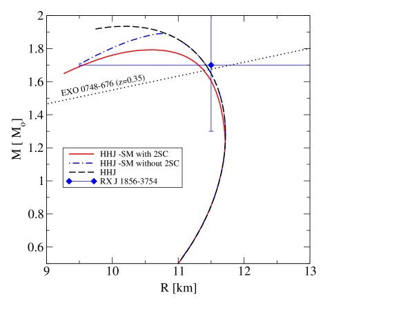
Figure 5: Mass - radius relations for compact star configurations with different EoS: purely hadronic star with HHJ EoS (dashed line), stable hybrid stars with HHJ - Gaussian nonlocal chiral quark separable model (SM) with 2SC phase (solid line) and with HHJ - SM, without 2SC phase (dash-dotted line). Data for two sources are also indicated, see [55, 56].

3 Heat transport, Neutrino production and diffusion

3.1 Boltzmann equation in curved space - time

For study of cooling evolution, we will use the diffusion approximation for neutrino transport, because it allows us easily to assess how global characteristics of the neutrino emission such as average energies, integrated fluxes, and time scales change in response to various input parameters. This approach is sufficient to establish connections between the microphysical ingredients and the duration of deleptonization and cooling time scales, which are necessary to estimate possible effects on neutrino signals. However, the detailed results of simulations for early cooling will not be presented in this lecture. The reader is referred to the works [57, 58] and citations within.

We will assume that the neutron star has an interior where the matter is spherically symmetric distributed. The evolution of the star will be assumed to be quasi stationary, which means that for each time step the velocity of the matter is zero.

The Boltzmann equation (BE) for massless particles is

$$p^{\beta}{\left({\frac{\partial f}{\partial x^{\beta}}}-{{\Gamma}_{\beta\gamma}^{\alpha}}p^{\gamma}{\frac{\partial f}{\partial p^{\alpha}}}\right)}={\left(\frac{df}{d\tau}\right)}_{coll}\,$$ (4)

where $f$ is the invariant neutrino distribution function, $p^{\alpha}$ is the neutrino 4-momentum and ${\Gamma}^{\alpha}_{\beta\gamma}$ are the Christoffel symbols for the metric

$$d\tau^{2}=-e^{2\phi}dt^{2}+e^{2\Lambda}dr^{2}+r^{2}d\theta^{2}+r^{2}\sin^{2}\theta\,d\Phi^{2}\,$$ (5)

of static spherically symmetric space-time manifold.

For simplicity one can use the comoving basis and rewrite the BE

$$p^{b}{\left({e^{\beta}_{b}}{\frac{\partial f}{\partial x^{\beta}}}-{\Gamma}^{a}_{bc}p^{c}{\frac{\partial f}{\partial p^{a}}}\right)}={\left(\frac{df}{d\tau}\right)}_{coll},$$ (6)

where ${e^{\beta}_{b}}$ are basis vectors in a comoving frame to an observer and in the static case they are diagonal. Indices $a,b,c$ are running from 0 to 3. The ${\Gamma}^{a}_{bc}$ are Ricci rotational coefficients with the non-zero components

$$\Gamma^{1}_{00} = {\Gamma}^{0}_{01}=e^{-\Lambda}\frac{\partial\phi}{\partial r},$$ (7)

$$\Gamma^{2}_{21} = -{\Gamma}^{1}_{22}=-{\Gamma}^{1}_{33}={\Gamma}^{3}_{31}={{e^{-\Lambda}}\over{r}},$$

$${\Gamma}^{2}_{33} = -{\Gamma}^{3}_{32}=-\frac{\cot\theta}{r}.$$

The neutrino 4-momentum is

$$p^{a}=\left(\omega,\omega{\mu},\omega{(1-{\mu}^{2})}^{1/2}\cos{\Phi},\omega{(1-{\mu}^{2})}^{1/2}\sin{\Phi}\right)\,,$$

where $\mu$ is the cosine of the angle between the neutrino momentum and the radial direction, $\omega$ is the neutrino energy in a comoving frame. Using the previous definitions we will have

$$\omega e^{t}_{0}\frac{\partial f}{\partial t} + \omega\mu e^{r}_{1}\frac{\partial f}{\partial r}-\omega^{2}{\mu}\Gamma^{1}_{00}\frac{\partial f}{\partial\omega}-\omega{(1-{\mu}^{2})}{\left(\Gamma^{1}_{00}+\Gamma^{1}_{22}\right)}\frac{\partial f}{\partial\mu}={\left(\frac{df}{d\tau}\right)}_{coll}\,.$$ (8)

3.1.1 Equations in Linear response Approximation

After applying the operator

$$\frac{1}{2}\int_{-1}^{+1}d{\mu}\,{\mu}^{i}\,,\quad i=0,1,2,\cdots,\;\;$$

to equation (8) and defining the $i^{\rm th}$ moments [59]

$$M_{i}=\frac{1}{2}\int_{-1}^{+1}d{\mu}\,{\mu}^{i}f,\;\;Q_{i}=\frac{1}{2}\int_{-1}^{+1}d{\mu}\,\mu^{i}{\left(\frac{df}{d\tau}\right)}_{coll}\,.$$

we get for $i=0$

$${\omega}\left({e^{t}_{0}}\frac{\partial M_{0}}{\partial t}+{e^{r}_{1}}\frac{\partial M_{1}}{\partial r}\right)-{\omega}^{2}{\left(\Gamma^{1}_{00}\frac{\partial M_{1}}{\partial{\omega}}\right)}-2{\omega}(\Gamma^{1}_{00}+\Gamma^{1}_{22})M_{1}=Q_{0},$$ (9)

and for $i=1$

$${\omega}\left({e^{t}_{0}}\frac{\partial M_{1}}{\partial t}+{e^{r}_{1}}\frac{\partial M_{2}}{\partial r}\right)-{\omega}^{2}{\left(\Gamma^{1}_{00}\frac{\partial M_{2}}{\partial{\omega}}\right)}+{\omega}(\Gamma^{1}_{00}+\Gamma^{1}_{22})(M_{0}-3M_{2})=Q_{1}\,.$$ (10)

Let us introduce $N_{\nu}$, $F_{\nu}$, and $S_{N}$ as the number density, number flux and the number source term, respectively,

$$N_{\nu}=\int_{0}^{\infty}\frac{d\omega}{2\pi^{2}}\,M_{0}\omega^{2}\,,\quad F_{\nu}=\int_{0}^{\infty}\frac{d\omega}{2\pi^{2}}\,M_{1}\omega^{2}\,,\quad S_{N}=\int_{0}^{\infty}\frac{d\omega}{2\pi^{2}}\,Q_{0}\omega,$$

while $J_{\nu}$, $H_{\nu}$, $P_{\nu}$, and $S_{E}$ are the neutrino energy density, energy flux, pressure, and the energy source term

$$J_{\nu} = \int_{0}^{\infty}\frac{d\omega}{2\pi^{2}}\,M_{0}\omega^{3}\,,\quad H_{\nu}=\int_{0}^{\infty}\frac{d\omega}{2\pi^{2}}\,M_{1}\omega^{3}\,,$$

$$P_{\nu} = \int_{0}^{\infty}\frac{d\omega}{2\pi^{2}}\,M_{2}\omega^{3}\,,\quad S_{E}=\int_{0}^{\infty}\frac{d\omega}{2\pi^{2}}\,Q_{0}\omega^{2}\,.$$ (11)

After integration over the neutrino energy and utilizing the continuity equation under assumption of a quasi-static evolution, one can recover the well known neutrino transport equation [60]

$$\frac{\partial({N_{\nu}/n_{B})}}{\partial t}+{\frac{\partial(e^{\phi}4\pi r^{2}F_{\nu})}{\partial a}}=e^{\phi}\frac{S_{N}}{n_{B}},$$ (12)

$$\frac{\partial({J_{\nu}/n_{B}})}{\partial t}+P_{\nu}\frac{\partial({1/n_{B}})}{\partial t}+e^{-\phi}{\frac{\partial(e^{2\phi}4\pi r^{2}H_{\nu})}{\partial a}}=e^{\phi}\frac{S_{E}}{n_{B}}\,.$$ (13)

The distribution function in the diffusion approximation could be represented in the following way

$$f(\omega,\mu)=f_{0}(\omega)+\mu f_{1}(\omega)\,,\quad f_{0}=[1+e^{\left(\frac{\omega-\mu_{\nu}}{kT}\right)}]^{-1}\,,$$ (14)

where $f_{0}(\omega)$ is the distribution function in equilibrium ($T=T_{mat}$, $\mu_{\nu}=\mu_{\nu}^{eq}$) with the neutrino energy $\omega$ and the chemical potential $\mu_{\nu}$ respectively. Hereafter the dependence of $f_{0}$ and $f_{1}$ on $\omega$ and non explicit dependence on space-time coordinates will be assumed without listing in arguments.

Thus the moments $M_{i}$ of the distribution function $f$ are

$$M_{0}=f_{0}\,,\,\,M_{1}=\frac{1}{3}f_{1}\,,\,\,M_{2}=\frac{1}{3}f_{0}\,,\,\,\quad{\rm and}\quad M_{3}=\frac{1}{5}f_{1}\,.$$ (15)

Therefore the equation (10) now reads

$${e^{-\Lambda}}\left(\frac{\partial f_{0}}{\partial r}-{\omega}{\frac{\partial\phi}{\partial r}}\frac{\partial f_{0}}{\partial\omega}\right)=3\frac{Q_{1}}{\omega}\,.$$ (16)

The collision term $Q_{1}$ can be represented as

$${\left(\frac{df}{d\tau}\right)}_{coll}=\omega\left(j_{a}(1-f)-\frac{f}{\lambda_{a}}+j_{s}(1-f)-\frac{f}{\lambda_{s}}\right)\,.$$ (17)

Here $j_{a}$ is the emissivity, $\lambda_{a}$ is the absorptivity, $j_{s}$ and $\lambda_{s}$ are the scattering contributions.

Namely

$$j_{s}=\frac{1}{{(2\pi)}^{3}}\int_{0}^{\infty}d\omega^{\prime}\,\omega^{\prime 2}\int_{-1}^{1}d\mu^{\prime}\int_{0}^{2\pi}d\Phi\,f(\omega^{\prime},\mu^{\prime})R^{in}_{s}(\omega,\omega^{\prime},\cos\theta)\,,$$ (18)

$$\frac{1}{\lambda_{s}}=\frac{1}{{(2\pi)}^{3}}\int_{0}^{\infty}d\omega^{\prime}\,\omega^{\prime 2}\int_{-1}^{1}d\mu^{\prime}\int_{0}^{2\pi}d\Phi\,[1-f(\omega^{\prime},\mu^{\prime})]R^{out}_{s}(\omega,\omega^{\prime},\cos\theta)\,,$$ (19)

where $\theta$ is the scattering angle. The relation between emissivities and absorptivities ($R^{in}_{s}$ and $R^{out}_{s}$ are scattering kernels) is given by

$$\frac{1}{\lambda_{a}(\omega)}=e^{\beta(\omega-\mu_{\nu}^{eq})}j_{a}(\omega)\quad{\rm and}\quad{R^{in}_{s}}=e^{\beta(\omega^{\prime}-\omega)}R^{out}_{s}\,.$$ (20)

Using the Legendre expansion for the moments one has

$$R^{out}_{l}=\int_{-1}^{1}d\cos{\theta}\,P_{l}(\cos\theta)R^{out}_{s}(\omega,\omega^{\prime},\cos{\theta})\,.$$ (21)

Performing the angular integrations of Eq. (17) one can define the relation between $Q_{0}$, $Q_{1}$ and $R^{out}_{0}$, $R^{out}_{1}$.

After substitution of the expression for $Q_{1}$ into Eq.(16) the relation between $f_{0}$ and $f_{1}$ reads

$$f_{1}=-D(\omega)\left[\frac{\partial f_{0}}{\partial r}-\omega\frac{\partial\phi}{\partial r}{\frac{\partial f_{0}}{\partial\omega}}\right]e^{-\Lambda}\,,D(\omega)={\left(j_{a}+\frac{1}{\lambda_{a}}+\kappa^{s}_{1}\right)}^{-1}\,,$$ (22)

where $D(\omega)$ is the diffusion coefficient. Using the relation between $\frac{\partial f_{0}}{\partial r}$ and $\frac{\partial f_{0}}{\partial\omega}$ and the notation $\eta=\mu_{\nu}/T$ to be the neutrino degeneracy parameter, we obtain

$$f_{1}=-D(\omega)e^{-\Lambda}\left[T\frac{\partial\eta}{\partial r}+\frac{\omega}{Te^{\phi}}\frac{\partial(Te^{\phi})}{\partial r}\right]\left(-\,\frac{\partial f_{0}}{\partial\omega}\right)\,.$$ (23)

Now the energy-integrated lepton and energy fluxes are

$$F_{\nu} = -\,\frac{e^{-\Lambda}e^{-\phi}T^{2}}{6\pi^{2}}\left[D_{3}\frac{\partial(Te^{\phi})}{\partial r}+(Te^{\phi})D_{2}\frac{\partial\eta}{\partial r}\right]$$

$$H_{\nu} = -\,\frac{e^{-\Lambda}e^{-\phi}T^{3}}{6\pi^{2}}\left[D_{4}\frac{\partial(Te^{\phi})}{\partial r}+(Te^{\phi})D_{3}\frac{\partial\eta}{\partial r}\right]\,.$$ (24)

Here the coefficients $D_{2}$, $D_{3}$, and $D_{4}$ are defined through the integrals over $\omega$ as

$$D_{n}=T^{-(n+1)}\,\int_{0}^{\infty}d\omega~{}\omega^{n}D(\omega)f_{0}(\omega)(1-f_{0}(\omega))~{}.$$

The explicit expression for the absorption mean free path is

$$\frac{1}{\lambda_{a}}=\frac{G_{F}^{2}}{\pi^{2}}\int_{0}^{\infty}dE_{e}\,E_{e}^{2}\,\left[1-f_{eq}(E_{e})\right]\int_{-1}^{+1}d\cos{\theta}\,\frac{(\cos\theta-1)}{1-e^{-z}}\left[AR_{1}+R_{2}+BR_{3}\right]$$ (25)

$$R^{out}_{s}={4G_{F}^{2}}\frac{(\cos\theta-1)}{1-e^{-z}}\left[AR_{1}+R_{2}+BR_{3}\right]$$ (26)

The response functions written in terms of the polarization functions are

$$R_{1} = ({\cal V}^{2}+{\cal A}^{2})~{}[{\rm Im}~{}\Pi^{R}_{L}(q_{0},q)+{\rm Im}~{}\Pi^{R}_{T}(q_{0},q)]$$ (27)

$$R_{2} = ({\cal V}^{2}+{\cal A}^{2})~{}{\rm Im}~{}\Pi^{R}_{T}(q_{0},q)-{\cal A}^{2}~{}{\rm Im}~{}\Pi^{R}_{A}(q_{0},q)$$ (28)

$$\;\;\;\;R_{3} = 2{\cal V}{\cal A}~{}{\rm Im}~{}\Pi^{R}_{VA}(q_{0},q)\,,$$ (29)

where the coupling constants for the absorption are ${\cal V}=g_{V}\cos(\theta_{c})$ and ${\cal A}=g_{A}\cos(\theta_{c})$ and for the scattering ${\cal V}=g_{V}/2$ and ${\cal A}=g_{A}/2$. $\theta_{c}$ is the Cabibbo angle, $g_{V}$ and $g_{A}$ are the vector and axial-vector couplings.

Introducing the $s$ entropy per baryon and $Y_{L}=(N_{\nu}+N_{e}+N_{\mu})/n_{B}$ lepton number fraction and with help of conservation laws for energy and baryon number combined with Eqs. (12) and (13) we finally will obtain the energy transport equation

$${T}e^{\phi}\frac{\partial{{s}}}{\partial{t}}+{\mu_{\nu}}e^{\phi}\frac{\partial{{Y_{L}}}}{\partial{t}}+\frac{\partial{(e^{2\phi}4\pi r^{2}{H_{\nu}})}}{\partial{a}}=0$$ (30)

and the equation for lepton diffusion

$$\frac{\partial{{Y_{L}}}}{\partial{t}}+\frac{\partial{(e^{\phi}4\pi r^{2}{F_{\nu}})}}{\partial{a}}=0.$$ (31)

The energy $H_{\nu}$ and lepton $F_{\nu}$ fluxes are defined in Eq.(24).

These coupled equations for the unknowns $T$ and $\mu_{\nu}$ with the Eq.(2) for the star structure completely describe the early cooling evolution of the compact objects in quasi-stationary regime. The solutions and more detailed information one can find in [57]. In the next section we will use the energy transport equation for consideration of late cooling evolution when the neutrinos are already untrapped, i.e. the mean free path $\lambda_{a}$ is larger than the star radius $R$ and $\mu_{\nu}=0$.

3.2 Late cooling evolution

The cooling scenario is described with a set of cooling regulators. In the regime without neutrino diffusion in the righthand side of Eq. (13) and therefore also in Eq. (30) for energy transport we introduce the energy loss term $\epsilon_{\nu}$ due to neutrino emission additional to $S_{E}$ and instead of the $H_{\nu}$ we use the total energy flux function $l(r,t)$. The temperature profile $T(r,t)$ is the one time dependent unknown dynamical quantity and during the cooling process due to an inhomogeneous distribution of the matter inside the star and the finite heat conductivity it can differ from the isothermal one. The heat conductivity $\kappa$ (the corresponding term to $D_{4}$ in Eq. (30)) determines the relation between $l(r,t)$ and gradient of $T(r,t)$. In isothermal age the temperature on the inner crust boundary ($T_{m}$) and the central temperature ($T_{c}$) are connected by the relation $T_{m}=T_{c}\exp[\phi(0)-\phi(R)]$. Here $\phi(0)-\phi(R)$ is the difference of the gravitational potentials in the center and at the surface of the star, respectively.

The flux of energy $l(r)$ per unit time through a spherical slice at the distance $r$ from the center, is proportional to the gradient of the temperature on both sides of this slice,

$$l(r)=-4\pi r^{2}\kappa(r)\frac{\partial(T{\rm e}^{\phi})}{\partial r}{\rm e}^{-\phi}\sqrt{1-\frac{2M}{r}}~{},$$ (32)

where the factor ${\rm e}^{-\phi}\sqrt{1-\frac{2M}{r}}$ corresponds to the relativistic correction of the time scale and the unit of thickness. The equations for energy balance and thermal energy transport are [3]

$$\frac{\partial}{\partial A}\left(l{\rm e}^{2\phi}\right) = -\frac{1}{n}\left(\epsilon_{\nu}{\rm e}^{2\phi}+c_{V}\frac{\partial}{\partial t}(T{\rm e}^{\phi})\right)~{},$$ (33)

$$\frac{\partial}{\partial A}\left(T{\rm e}^{\phi}\right) = -\frac{1}{\kappa}\frac{l{\rm e}^{\phi}}{16\pi^{2}r^{4}n}~{},$$ (34)

where $n=n(r)$ is the baryon number density, $A=A(r)$ is the total baryon number within a sphere of radius $r$. One has

$$\frac{\partial r}{\partial A}=\frac{1}{4\pi r^{2}n}\sqrt{1-\frac{2M}{r}}~{}.$$ (35)

The total neutrino emissivity $\epsilon_{\nu}$ and the total specific heat $c_{V}$ are given as the sum of the corresponding partial contributions defined in the next subsections. The density profiles $n_{i}(r)$ of the constituents $i$ of the matter are under the conditions of the actual temperature profile $T(r,t)$. The accumulated mass $M=M(r)$ and the gravitational potential $\phi=\phi(r)$ can be determined by

$$\frac{\partial M}{\partial A} = \frac{\varepsilon}{n}\sqrt{1-\frac{2M}{r}}~{},$$ (36)

$$\frac{\partial\phi}{\partial A} = \frac{4\pi r^{3}p+M}{4\pi r^{2}n}\frac{1}{\sqrt{1-\frac{2M}{r}}}~{},$$ (37)

where the energy density profile $\varepsilon=\varepsilon(r)$ and the pressure profile $p=p(r)$ is defined by the condition of hydrodynamical equilibrium (see Eq. 2)

$$\frac{\partial p}{\partial A}=-(p+\varepsilon)\frac{\partial\phi}{\partial A}~{}.$$ (38)

The boundary conditions for the solution of (33) and (34) read $l(r=0)=l(A=0)=0$ and $T(A(r_{m})=A,t)=T(r_{m}=R,t)=T_{m}(t)$, respectively.

In our examples we choose the initial temperature to be 1 MeV. This is a typical value for the temperature $T_{\rm opacity}$ at which the star becomes transparent for neutrinos. Simplifying we disregard the neutrino influence on transport. These effects dominate for $t<1\div 100$ min, when the star cools down to $T\leq T_{\rm opacity}$ and become unimportant for later times.

3.2.1 Neutrino Processes in dense matter

We compute the NS thermal evolution adopting our fully general relativistic evolutionary code. This code was originally constructed for the description of hybrid stars by [17]. The main cooling regulators are the thermal conductivity, the heat capacity and the emissivity.

Emissivity

The luminosities are calculated using the corresponding matrix element of the neutrino production process

$$L_{\nu}=(2\pi)^{4}\int\frac{d^{3}p_{n}}{(2\pi)^{3}2E_{n}}\dots\int\frac{d^{3}p_{\nu}}{(2\pi)^{3}2E_{\nu}}~{}\delta^{3}(\vec{p}_{i})\delta(E_{i})~{}\big{|}M_{fi}\big{|}^{2}~{}f_{n}(1-f_{p})(1-f_{e}).$$ (39)

The most effective process of neutrino production is the direct Urca (DU) one, $n\longrightarrow p+e^{-}+\bar{\nu}_{e}$, which is allowed when the momentum conservation holds  $\vec{p}_{F,n}=\vec{p}_{F,p}+\vec{p}_{F,e}$   $\Leftrightarrow$   $|\vec{p}_{F,n}|\leq|\vec{p}_{F,p}|+|\vec{p}_{F,e}|$. Since DU process is so intensive that as soon as it takes place the star cools too fast for better correspondence between the cooling simulations and the observational data, it is likely to assumed DU to be forbidden in the interior of the star.

The other processes, i.e. the modified Urca (MU), pair breaking and formation (PBF) and bremsstrahlung are the main ones governing the cooling in hadronic matter. The modified Urca (MU) $nn\rightarrow npe\bar{\nu}$, $np\rightarrow ppe\bar{\nu}$, has to be medium modified Urca (MMU) process due to the softening of in-medium pion propagator. The final emissivity is given by [9, 62]

$$\epsilon_{\nu}^{\rm nMU} = 8.6\times 10^{21}m^{*4}_{\rm nMU}(Y_{e}u)^{1/3}\zeta_{\rm nMU}T_{9}^{8}{\rm ergcm^{-3}s^{-1}},$$ (40)

$$\epsilon_{\nu}^{\rm pMU} = 8.5\times 10^{21}m^{*4}_{\rm pMU}(Y_{e}u)^{1/3}\zeta_{\rm pMU}T_{9}^{8}{\rm ergcm^{-3}s^{-1}}.$$ (41)

Here $m_{i}^{*}=\sqrt{m_{{\rm{rel}},i}^{*2}+p_{{\rm{F}},i}^{2}}$ is the non-relativistic quasiparticle effective mass related to the in-medium one-particle energies from a given relativistic mean field model for $i=n,p$. We have introduced the abbreviations $m^{*4}_{\rm nMU}=({m_{n}^{*}}/{m_{n}})^{3}({m_{p}^{*}}/{m_{p}})$ and $m^{*4}_{pMU}=({m_{p}^{*}}/{m_{p}})^{3}({m_{n}^{*}}/{m_{n}})$. The suppression factors are $\zeta_{\rm nMU}=\zeta_{n}\zeta_{p}\simeq{\exp}\{-[\Delta_{n}(T)+\Delta_{p}(T)]/T\}$, $\zeta_{\rm pMU}\simeq\zeta_{p}^{2}$, and should be replaced by unity for $T>T_{{\rm crit},i}$, when for given species $i$ the corresponding gap vanishes. For neutron and proton $S$-wave pairing is $\Delta_{i}(0)=1.76~{}T_{{\rm crit},i}$ and for the $P$-wave pairing of neutrons $\Delta_{n}(0)=1.19~{}T_{{\rm crit},n}$ (see Fig. 6). The gap as a function of temperature is given by the interpolation formula $\Delta_{N}(T)=\Delta(0)\sqrt{1-T/T_{{\rm crit},N}}$.

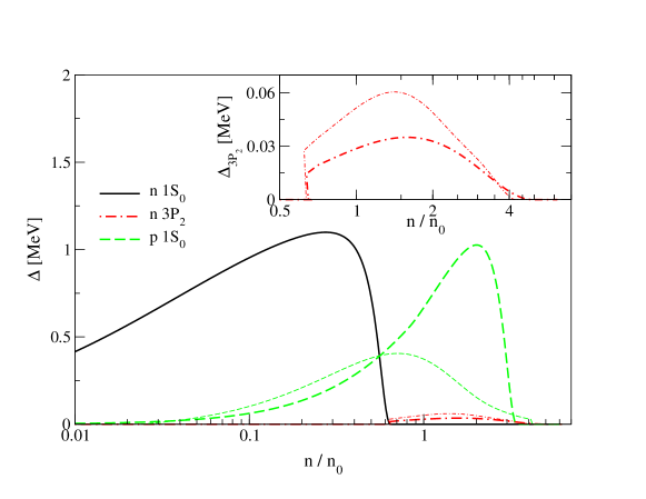
Figure 6: Neutron and proton pairing gaps according to model I (thick solid, dashed and dotted lines) and according to model II (thin lines), see text. The $1S_{0}$ neutron gap is the same in both models, taken from [64].

To be conservative we have used in (40) the free one-pion exchange estimate of the $NN$ interaction amplitude. Restricting ourselves to a qualitative analysis we use here simplified exponential suppression factors $\zeta_{i}$. In a more detailed analysis these $\zeta_{i}$-factors have prefactors with rather strong temperature dependences [62]. At temperatures $T\sim T_{c}$ their inclusion only slightly affects the resulting cooling curves. For $T\ll T_{c}$ the MU process gives in any case a negligible contribution to the total emissivity and thereby corresponding modifications can again be omitted. Also for the sake of simplicity the general possibility of a ³P${}_{2}(|m_{J}|=2)$ pairing which may result in a power-law behaviour of the specific heat and the emissivity of the MU process [61, 62, 63] is disregarded since mechanisms of this type of pairing are up to now not elaborated. Even more essential modifications of the MU rates may presumably come from in-medium effects which could result in extra prefactors of $10^{2}\div 10^{3}$ already at $T\sim T_{c}$.

In order to estimate the role of the in-medium effects in the $NN$ interaction for the HNS cooling we have also performed calculations for the so-called medium modified Urca (MMU) process [65, 66] by multiplying the rates (40) by the appropriate prefactor

$$\epsilon_{\nu}^{\rm MMU}/\epsilon_{\nu}^{\rm MU}\simeq 10^{3}\left[\Gamma^{6}(g^{\prime})/\widetilde{\omega}^{8}(k\simeq p_{F})\right]u^{10/3},$$ (42)

where the value $\Gamma(g^{\prime})\simeq 1/[1+1.4~{}u^{1/3}]$ is due to the dressing of $\pi NN$ vertices and $\widetilde{\omega}\leq m_{\pi}$ is the effective pion gap which we took as function of density from Fig. 2 of [67].

For $T<T_{\rm crit}$ the most important contribution comes from the neutron [63, 62] and the proton [63] pair breaking and formation processes. We take their emissivities from Ref. [67], which is applicable for both cases, $S$- and $P$-wave nucleon pairing

$$\epsilon_{\nu}^{\rm nPBF} = 6.6\times 10^{28}({m_{n}^{*}}/{m_{n}})({\Delta_{n}(T)}/{\rm MeV})^{7}~{}u^{1/3}$$ (43)

$$\times\xi~{}I({\Delta_{n}(T)}/{T})~{}{\rm erg~{}cm^{-3}s^{-1}},$$

$$\epsilon_{\nu}^{\rm pPBF} = 0.8\times 10^{28}({m_{p}^{*}}/{m_{p}})({\Delta_{p}(T)}/{\rm MeV})^{7}~{}u^{2/3}$$ (44)

$$\times~{}I({\Delta_{p}(T)}/{T})~{}{\rm erg~{}cm^{-3}s^{-1}},$$

where

$$I({\Delta_{i}(T)}/{T})\simeq 0.89~{}\sqrt{T/\Delta_{i}(T)}\exp[-2\Delta_{i}(T)/T]~{},$$ (45)

$\xi\simeq 0.5$ for ${}^{1}S_{0}$ pairing and $\xi\simeq 1$ for ${}^{3}P_{2}$ pairing.

A significant contribution of the proton channel is due to the $NN$ correlation effects, which are taken into account in [63].

The phonon contribution to the emissivity of the $3P_{2}$ superfluid phase is negligible. The main emissivity regulators are the MMU Eq. (42) and the neutron (nPBF) and proton (pPBF) pair breaking and formation processes Eq. (43), see above for a rough estimation. Finally, we include the effect of a pion condensate (PU process), where the PU emissivity is about 1-2 orders of magnitude smaller than the DU one.

All emissivities are corrected by correlation effects. We adopt the same set of partial emissivities as in the work of [67].

In quark matter the process $d\longrightarrow u+e^{-}+\bar{\nu}_{e}$ is always allowed unless it is suppressed by huge energy gaps due to quark pairing.

$$\epsilon^{\rm QDU}_{\nu}\simeq 9.4\times 10^{26}\alpha_{s}uY_{e}^{1/3}\zeta_{\rm QDU}~{}T_{9}^{6}~{}{\rm erg~{}cm^{-3}~{}s^{-1}},$$ (46)

where at a compression $u=n/n_{0}\simeq 2$ the strong coupling constant is $\alpha_{s}\approx 1$ and decreases logarithmically at still higher densities. The nuclear saturation density is $n_{0}=0.17~{}{\rm fm}^{-3}$, $Y_{e}=n_{e}/n$ is the electron fraction, and $T_{9}$ is the temperature in units of $10^{9}$ K. If, for a somewhat higher density, the electron fraction was too small ($Y_{e}<Y_{ec}\simeq 10^{-8}$), then all the QDU processes would be completely switched off [68] and the neutrino emission would be governed by two-quark reactions like the quark modified Urca (QMU) and the quark bremsstrahlung (QB) processes $dq\rightarrow uqe\bar{\nu}$ and $q_{1}q_{2}\rightarrow q_{1}q_{2}\nu\bar{\nu}$, respectively. The emissivities of the QMU and QB processes have been estimated as [69]

$$\epsilon^{\rm QMU}_{\nu}\sim\epsilon^{\rm QB}_{\nu}\simeq 9.0\times 10^{19}\zeta_{\rm QMU}~{}T_{9}^{8}~{}{\rm erg~{}cm^{-3}~{}s^{-1}}.$$ (47)

Due to the pairing, the emissivities of QDU processes are suppressed by a factor $\zeta_{\rm QDU}\sim\mbox{exp}(-\Delta_{q}/T)$ and the emissivities of QMU and QB processes are suppressed by a factor $\zeta_{\rm QMU}\sim\mbox{exp}(-2\Delta_{q}/T)$ for $T<T_{{\rm crit},q}\simeq 0.4~{}\Delta_{q}$ whereas for $T>T_{{\rm crit},q}$ these factors are equal to unity. The modification of $T_{{\rm crit},q}(\Delta_{q})$ relative to the standard BCS formula is due to the formation of correlations as, e.g., instanton- anti-instanton molecules [71]. For the temperature dependence of the gap below $T_{{\rm crit},q}$ we use the interpolation formula $\Delta(T)=\Delta(0)\sqrt{1-T/T_{{\rm crit},q}}$, with $\Delta(0)$ being the gap at zero temperature.

The contribution of the reaction $ee\rightarrow ee\nu\bar{\nu}$ is very small [70]

$$\epsilon^{ee}_{\nu}=2.8\times 10^{12}\,Y_{e}^{1/3}u^{1/3}T_{9}^{8}~{}{\rm erg~{}cm^{-3}~{}s^{-1}},$$ (48)

but can become important, when quark processes are blocked out for large values of $\Delta_{q}/T$ in superconducting quark matter.

Thermal conductivity

The heat conductivity of the matter is the sum of the partial contributions [72, 73]

$$\kappa=\sum_{i}\kappa_{i},\,\,\,\frac{1}{\kappa_{i}}=\sum_{j}\frac{1}{\kappa_{ij}}~{},$$ (49)

where $i,j$ denote the components (particle species).

The contribution of neutrons and protons is

$$\kappa_{nn} = 8.3\times 10^{22}\left(\frac{m_{n}}{m_{n}^{*}}\right)^{4}\frac{z_{n}^{3}~{}\zeta_{n}}{S_{kn}~{}T_{9}}~{}{\rm erg~{}s^{-1}cm^{-1}K^{-1}},$$ (50)

$$S_{kn} = 0.38~{}z_{n}^{-7/2}+3.7~{}z_{n}^{2/5}~{},$$ (51)

$$\kappa_{np} = 8.9\times 10^{16}\left(\frac{m_{n}}{m_{n}^{*}}\right)^{2}\frac{z_{n}^{2}\zeta_{p}T_{9}}{z_{p}^{3}S_{kp}}~{}{\rm erg~{}s^{-1}cm^{-1}K^{-1}},$$ (52)

$$S_{kp} = 1.83~{}z_{n}^{-2}+1.43~{}z_{n}^{2}(0.4+z_{n}^{8})^{-1}~{}.$$ (53)

Here we have introduced the appropriate suppression factors $\zeta_{i}$ which act in the presence of gaps for superfluid hadronic matter (see Fig. 6) and we have used the abbreviation $z_{i}=(n_{i}/(4n_{0}))^{1/3}$. The heat conductivity of electrons is given by Eq. (56). The total contribution related to electrons is then

$$1/\kappa_{e}=1/\kappa_{ee}+1/\kappa_{ep}.$$ (54)

Similar expressions we have for neutrons and protons using Eqs. (50)-(53).

The total thermal conductivity is the straight sum of the partial contributions $\kappa_{tot}=\kappa_{e}+\kappa_{n}+...$ . Other contributions to this sum are smaller than those presented explicitly ($\kappa_{e}$ and $\kappa_{n}$).

For quark matter $\kappa$ is the sum of the partial conductivities of the electron, quark and gluon components [73, 74]

$$\kappa=\kappa_{e}+\kappa_{q}+\kappa_{g},$$ (55)

where $\kappa_{e}\simeq\kappa_{ee}$ is determined by electron-electron scattering processes since in superconducting quark matter the partial contribution $1/\kappa_{eq}$ (as well as $1/\kappa_{gq}$ ) is additionally suppressed by a $\zeta_{\rm QDU}$ factor, as for the scattering on impurities in metallic superconductors. For $\kappa_{ee}$ we have

$$\kappa_{ee} = 5.5\times 10^{23}u~{}{Y_{e}}~{}{T_{9}}^{-1}~{}{\rm erg~{}s^{-1}cm^{-1}K^{-1}},$$ (56)

and

$$\kappa_{q}\simeq\kappa_{qq}\simeq 1.1\times 10^{23}\sqrt{\frac{4\pi}{\alpha_{s}}}~{}u~{}\zeta_{\rm QDU}{T_{9}}^{-1}{\rm erg~{}s^{-1}cm^{-1}K^{-1}},$$ (57)

where we take into account the suppression factor. We estimate the contribution of massless gluons as

$$\kappa_{g}\simeq\kappa_{gg}\simeq 6.0\times 10^{17}~{}T_{9}^{2}~{}{\rm erg~{}s^{-1}cm^{-1}K^{-1}}.$$ (58)

Heat capacity

The heat capacity contains nucleon, electron, photon, phonon, and other contributions. The main in-medium modification of the nucleon heat capacity is due to the density dependence of the effective nucleon mass. We use the same expressions as [67]. The main regulators are the nucleon and the electron contributions. For the nucleons ($i=n,p$), the specific heat is [9]

$$c_{i}\sim 1.6\times 10^{20}({m_{i}^{*}}/{m_{i}})~{}(n_{i}/n_{0})^{1/3}\zeta_{ii}~{}T_{9}~{}{\rm erg~{}cm^{-3}K^{-1}}~{},$$ (59)

and for the electrons it is

$$c_{e}\sim 6\times 10^{19}\,(n_{e}/n_{0})^{2/3}~{}T_{9}~{}{\rm erg~{}cm^{-3}~{}K^{-1}}~{}.$$ (60)

Near the phase transition point the heat capacity acquires a fluctuation contribution. For the first order pion condensation phase transition this additional contribution contains no singularity, unlike the second order phase transition, see [66]. Finally, the nucleon contribution to the heat capacity may increase up to several times in the vicinity of the pion condensation point. The effect of this correction on global cooling properties is rather unimportant.

The symmetry of the $3P_{2}$ superfluid phase allows a Goldstone boson (phonon) contribution of

$$c_{G}\simeq 6\cdot 10^{14}T_{9}^{3}\,\,\,{\rm erg}\,{\rm cm}^{-3}~{}{\rm K^{-1}},$$ (61)

for $T<T_{cn}(3P_{2})$, $n>n_{cn}(3P_{2})$. We include this contribution in our study too, although its effect on the cooling is rather minor.

For the quark specific heat we use the expression [69]

$$c_{q}\simeq 10^{21}u^{2/3}\zeta_{\rm S}~{}T_{9}~{}{\rm erg~{}cm^{-3}~{}K^{-1}},$$ (62)

where $\zeta_{\rm S}\simeq 3.1~{}(T_{{\rm crit},q}/T)^{5/2}~{}\mbox{exp}(-\Delta_{q}/T)$. Besides, one should add the gluon-photon contribution [15]

$$c_{g-\gamma}=3.0\times 10^{13}~{}N_{g-\gamma}~{}T_{9}^{3}~{}{\rm erg~{}cm^{-3}~{}K^{-1}},$$ (63)

where $N_{g-\gamma}$ is the number of available massless gluon-photon states (which are present even in the color superconducting phase), as well as the electron contribution,

$$c_{e}=5.7\times 10^{19}\,Y_{e}^{2/3}u^{2/3}~{}T_{9}~{}{\rm erg~{}cm^{-3}~{}K^{-1}}.$$ (64)

4 Results of simulations for Cooling evolution

We compute the neutron star thermal evolution adopting our fully general relativistic evolutionary code. The code originally constructed for the description of hybrid stars by [17] has been developed and updated according to the modern knowledge of inputs in [18].

The density $n\sim 0.5\div 0.7~{}n_{0}$ is the boundary of the neutron star interior and the inner crust. The latter is constructed of a pasta phase discussed by [75], see also recent works of [76, 77].

Further on we need a relation between the crust and the surface temperature for neutron star. A sharp change of the temperature occurs in the envelope. This $T_{\rm s}-T_{\rm in}$ relation has been calculated in several works, see [78, 79], depending on the assumed value of the magnetic field at the surface and some uncertainties in our knowledge of the structure of the envelope. For applications we use three different approximations: the simplified “Tsuruta law” $T_{\rm s}^{\rm Tsur}=(10~{}T_{\rm in})^{2/3}$ used in many old cooling calculations, models used by Ref. [79], and our fit formula interpolating two extreme curves describing the borders of region of available $T_{\rm s}-T_{\rm in}$ relation, taken from [79] (see Fig. 4 of Ref. [80]).

4.1 Cooling Evolution of Hadronic Stars

Here we will shortly summarize the results on hadronic cooling.

In framework of a ”minimal cooling” scenario, the pair breaking and formation (PBF) processes may allow to cover an ”intermediate cooling” group of data (even if one artificially suppressed medium effects)[67]. These processes are very efficient for large pairing gaps and temperatures being not much less than the value of the gap.

Gaps, which we have adopted in the framework of the ”nuclear medium cooling” scenario, see [80], are presented in Fig. 6. Thick dashed lines show proton gaps which were used in the work of [8] performed in the framework of the “standard plus exotics” scenario. We will call the choice of the “3nt” model from [8] the model I. Thin lines show $1S_{0}$ proton and $3P_{2}$ neutron gaps from [81], for the model AV18 by [82] (we call it the model II). Recently [83] has argued for a strong suppression of the $3P_{2}$ neutron gaps, down to values $\sim 10~{}$ keV, as the consequence of the medium-induced spin-orbit interaction.

These findings motivated [80] to suppress values of $3P_{2}$ gaps shown in Fig. 6 by an extra factor $f(3P_{2},n)=0.1$. Further possible suppression of the $3P_{2}$ gap is almost not reflected on the behavior of the cooling curves.

Contrary to expectations of [83] a more recent work of [84] argued that the $3P_{2}$ neutron pairing gap should be dramatically enhanced, as the consequence of the strong softening of the pion propagator. According to their estimate, the $3P_{2}$ neutron pairing gap is as large as $1\div 10$ MeV in a broad region of densities, see Fig. 1 of their work. Thus results of calculations of [83] and [84], which both had the same aim to include medium effects in the evaluation of the $3P_{2}$ neutron gaps, are in a deep discrepancy with each other.

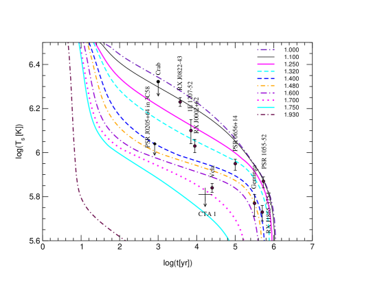
Figure 7: Cooling curves for the gaps from Fig. 6 for model II (the same as Fig. 21 of [80]). The original $3P_{2}$ neutron pairing gap is additionally suppressed by a factor $f(3P_{2},n)=0.1$. The $T_{\rm s}-T_{\rm in}$ relation is given by “our fit” curve of Fig. 4 in [80]. For more details see [80].

• Including superfluid gaps we see, in agreement with recent microscopic findings of [83], that the $3P_{2}$ neutron gap should be as small as $10$ keV or less. So the “nuclear medium cooling” scenario of [80] supports results of [83] and fails to appropriately fit the neutron star cooling data when a strong enhancement of the $3P_{2}$ neutron gaps is assumed as shown by [85].

• Medium effects associated with the pion softening are called for by the data. As the result of the pion softening the pion condensation may occur for $n\geq n_{c}^{\rm PU}$ ($n\geq 3n_{0}$ in our model). Its appearance at such rather high densities does not contradict to the cooling data (see Fig. 7), but also the data are well described using the pion softening but without assumption on the pion condensation. The similar argumentation holds also for DU threshold density. That puts restrictions on the density dependence of the symmetry energy. Both statements might be important in the discussion of the heavy ion collision experiments.

• We demonstrated a regular mass dependence for neutron stars with masses $M>1~{}M_{\odot}$, where less massive neutron stars cool down slower and more massive neutron stars cool faster. This feature is more general and concerning also to hybrid stars [86].

4.2 Cooling Evolution of Hybrid Stars with 2SC Quark Matter Core

For the calculation of the cooling of the quark core in the hybrid star we use the model [18]. We incorporate the most efficient processes: the quark direct Urca (QDU) processes on unpaired quarks, the quark modified Urca (QMU), the quark bremsstrahlung (QB), the electron bremsstrahlung (EB), and the massive gluon-photon decay (see [15]). Following [87] we include the emissivity of the quark pair formation and breaking (QPFB) processes, too. The specific heat incorporates the quark contribution, the electron contribution and the massless and massive gluon-photon contributions. The heat conductivity contains quark, electron and gluon terms.

The calculations are based on the hadronic cooling scenario presented in Fig. 7 and we add the contribution of the quark core. For the Gaussian form-factor the quark core occurs already for $M>1.214~{}M_{\odot}$ according to the model [47], see Fig. 5. Most of the relevant neutron star configurations (see Fig. 7) are then affected by the presence of the quark core.

First we check the possibility of the 2SC+ normal quark phases, see Fig. 8.

Figure 8: Model I. Cooling curves for hybrid star configurations with Gaussian quark matter core in the 2SC phase. The labels correspond to the gravitational masses of the configurations in units of the solar mass.

The variation of the gaps for the strong pairing of quarks within the 2SC phase and the gluon-photon mass in the interval $m_{g-\gamma}\sim 20\div 200~{}$MeV only slightly affects the results. The main cooling process is the QDU process on normal quarks. We see that the presence of normal quarks entails too fast cooling. The data could be explained only, if all the masses lie in a very narrow interval ($1.21<M/M_{\odot}<1.22$ in our case). In case of the other two crust models the resulting picture is similar.

The existence of only a very narrow mass interval, in which the data can be fitted seems to us unrealistic by itself. Moreover the observations show existence of neutron stars in binary systems with very different masses, e.g., $M_{\rm B1913+16}\simeq 1.4408\pm 0.0003~{}M_{\odot}$ and $M_{\rm J0737-3039B}\simeq 1.250\pm 0.005~{}M_{\odot}$, cf. [88]. Thus the data can’t be satisfactorily explained.

Then we assume a possibility of an yet unknown X-pairing channel with a small $\Delta_{X}$ gap and first check the case $\Delta_{X}$ to be constant. For $\Delta_{X}\simeq 1~{}$MeV the cooling is too slow [18]. This is true for all three crust models. Thus the gaps for formerly unpaired quarks should be still smaller in order to obtain a satisfactory description of the cooling data.

For the $\Delta_{X}=30~{}$ keV the cooling data can be fitted but have a very fragile dependence on the gravitational mass of the configuration. Namely, we see that all data points, except the Vela, CTA 1 and Geminga, correspond to hybrid stars with masses in the narrow interval $M=1.21\div 1.22~{}M_{\odot}$

Therefore we would like to explore whether a density-dependent X-gap could allow a description of the cooling data within a larger interval of compact star masses.

We employ an ansatz for the X-gap as a decreasing function of the chemical potential

$$\Delta_{X}(\mu)=\Delta_{c}~{}\exp[-\alpha(\mu-\mu_{c})/\mu_{c}]~{},$$ (65)

where the parameters are chosen such that at the critical quark chemical potential $\mu_{c}=330$ MeV the onset of the deconfinement phase transition for the X-gap has its maximal value of $\Delta_{c}=1.0$ MeV and at the highest attainable chemical potential $\mu_{\rm max}=507$ MeV, i.e. in the center of the maximum mass hybrid star configuration, it falls to a value of the order of $10$ keV. We choose the value $\alpha=10$ for which $\Delta_{X}(\mu_{\rm max})=4.6$ keV. In Fig. 9 we show the resulting cooling curves for the gap model II with gap ansatz eq. (65), which we consider as the most realistic one.

We observe that the mass interval for compact stars which obeys the cooling data is constrained between $M=1.32~{}M_{\odot}$ for slow coolers and $M=1.75~{}M_{\odot}$ for fast coolers such as Vela. This results we obtain are based on a purely hadronic model with different choices of the parameters [80]. Note that according to a recently suggested independent test of cooling models [89] by comparing results of a corresponding population synthesis model with the Log N - Log S distribution of nearby isolated X-ray sources the cooling model I did not pass the test. Thereby it would be interesting to see, whether our quark model within the gap ansatz II could pass the Log N - Log S test.

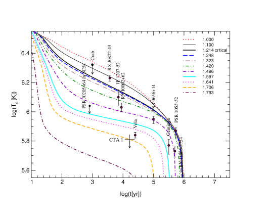
Figure 9: Cooling curves for hybrid star configurations with Gaussian quark matter core in the 2SC phase with a density dependent pairing gap according to Eq. (65) for model II.

5 Conclusions

In this lecture devoted to the modern problems of the cooling evolution of neutron stars we have discussed different successful scenarios aiming to explain the known temperature - age data from observations of compact objects. Using up today known theoretical and experimental constraints on the structure and cooling regulators of compact star we end up with alternative explanations. The neutron star can be either pure hadronic or hybrid one with a quark core in superconducting state of matter.

Particularly, for the hybrid stars, which are more intrigued alternative of superdense compact objects we conclude that:

• Within a nonlocal, chiral quark model the critical densities for a phase transition to color superconducting quark matter can be low enough for these phases to occur in compact star configurations with masses below $1.3~{}M_{\odot}$.

• For the choice of the Gaussian form-factor the 2SC quark matter phase arises at $M\simeq 1.21~{}M_{\odot}$.

• Without a residual pairing the 2SC quark matter phase could describe the cooling data only if compact stars had masses in a very narrow band around the critical mass for which the quark core can occur.

• Under assumption that formally unpaired quarks can be paired with small gaps $\Delta_{X}<1~{}$MeV (2SC+X pairing), which values we varied in wide limits, only for density dependent gaps the cooling data can be appropriately fitted.

So the present day cooling data could be still explained by hybrid stars, assuming a complex pairing pattern, where quarks are partly strongly paired within the 2SC channel, and partly weakly paired with gaps $\Delta_{X}<1~{}$MeV, which are rapidly decrease with an increase of the density.

It remains to be investigated which microscopic pairing pattern could fulfill the constraints obtained in this work. Another indirect check of the model could be the Log N - Log S test.

Acknowledgments

The research has been supported by the Virtual Institute of the Helmholtz Association under grant No. VH-VI-041 and by the DAAD partnership programm between the Universities of Yerevan and Rostock. In particular I acknowledge D. Blaschke for his active collaboration and support. I thank my colleagues D. Blaschke, D.N. Voskresensky, D.N. Aguilera, J. Berdermann, and A. Reichel for collaboration and discussions. I also thank the organizers of the organizers of the Helmholtz International Summer School and Workshop on Hot points in Astrophysics and Cosmology for their invitation to present these lectures.

————

References

- [1] S. L. Shapiro and S. A. Teukolsky, Black Holes, White Dwarfs, And Neutron Stars (Wiley, New York, 1983).
- [2] N. K. Glendenning, Compact Stars, (New York: Springer, 1996); N. K. Glendenning, Compact Stars: Nuclear Physics, Particle Physics, And General Relativity, (Springer, New York & London, 2000).
- [3] F. Weber, Pulsars as Astrophysical Laboratories for Nuclear and Particle Physics, (Bristol: IoP Publishing, 1999).
- [4] D. Page, J. M. Lattimer, M. Prakash and A. W. Steiner, Astrophys.J., Supliment, arXiv:astro-ph/0403657, (2004).
- [5] S. Tsuruta, M. A. Teter, T. Takatsuka, T. Tatsumi and R. Tamagaki, Astrophys. J. 571, (2002) L143.
- [6] S. Tsuruta, in: Proceedings of IAU Symposium “Young Neutron Stars, and their Environments”, F. Camilo, B.M. Gaensler (Eds.), 218, (2004).
- [7] A. D. Kaminker, D. G. Yakovlev and O. Y. Gnedin, arXiv:astro-ph/0111429, (2001).
- [8] D. G. Yakovlev, O. Y. Gnedin, A. D. Kaminker, K. P. Levenfish and A. Y. Potekhin, Adv. Space Res. 33, (2004) 523.
- [9] B. Friman, and O. V. Maxwell, Astrophys. J, 232 (1979) 541.
- [10] S. Tsuruta, Phys. Rep., 56, (1979) 237.
- [11] M. G. Alford, Ann. Rev. Nucl. Part. Sci. 51, (2001) 131.
- [12] M. Kitazawa, T. Koide, T. Kunihiro and Y. Nemoto, Phys. Rev. D 65, (2002) 091504.
- [13] D. N. Voskresensky, Phys. Rev. C 69, (2004) 065209.
- [14] D. Blaschke, N.K. Glendenning, A. Sedrakian (Eds.), Physics of Neutron Star Interiors, Springer, Berlin (2001).
- [15] D. Blaschke, T. Klähn and D. N. Voskresensky, Astrophys. J. 533, (2000) 406.
- [16] D. Page, M. Prakash, J. M. Lattimer and A. Steiner, Phys. Rev. Lett. 85, (2000) 2048.
- [17] D. Blaschke, H. Grigorian and D. N. Voskresensky, Astron. Astrophys. 368, (2001) 561.
- [18] H. Grigorian, D. Blaschke and D. Voskresensky, Phys. Rev. C 71, (2005) 045801; D. Blaschke, D. N. Voskresensky and H. Grigorian, arXiv:astro-ph/0403171. (2005)
- [19] A. Bender, D. Blaschke, Y. Kalinovsky and C. D. Roberts, Phys. Rev. Lett. 77, (1996) 3724; D. Blaschke, C. D. Roberts and S. M. Schmidt, Phys. Lett. B 425, (1998) 232; C. D. Roberts and S. M. Schmidt, Prog. Part. Nucl. Phys. 45, (2000) S1.
- [20] D. Blaschke, H. Grigorian, G. S. Poghosyan, C. D. Roberts and S. M. Schmidt, Phys. Lett. B 450, (1999) 207.
- [21] J. C. R. Bloch, C. D. Roberts and S. M. Schmidt, Phys. Rev. C 60, (1999) 065208.
- [22] G. V. Carter, S. Reddy, Phys. Rev. D 62, (2000) 103002.
- [23] M. Alford, K. Rajagopal, and F. Wilczek, Phys. Lett. B 422, (1998) 147.
- [24] R. Rapp, T. Schäfer, E.V. Shuryak, and M. Velkovsky, Phys. Rev. Lett. 81, (1998) 53.
- [25] A. Akmal, V.R. Pandharipande, and D.G. Ravenhall, Phys. Rev. C 58, (1998) 1804.
- [26] M. Baldo, I. Bombaci and G. F. Burgio, Astron. Astrophys. 328, (1997) 274.
- [27] W. Zuo, A. Lejeune, U. Lombardo and J. F. Mathiot, Nucl. Phys. A 706, (2002) 418.
- [28] H. Heiselberg and M. Hjorth-Jensen, Astrophys. J. 525, (1999) L45.
- [29] T. Gaitanos, M. Di Toro, S. Typel, V. Baran, C. Fuchs, V. Greco and H. H. Wolter, Nucl. Phys. A 732, (2004) 24.
- [30] E.N.E. van Dalen, C. Fuchs, and A. Faessler, Nucl. Phys. A 744, (2004) 227.
- [31] S. Typel, arXiv:nucl-th/0501056, (2005).
- [32] E. E. Kolomeitsev and D. N. Voskresensky, Phys. Rev. C 68, (2003) 015803.
- [33] M. Alford, K. Rajagopal and F. Wilczek, Phys. Lett. B 450, (1999) 325.
- [34] D. Blaschke and C. D. Roberts, Nucl. Phys. A 642, (1998) 197.
- [35] K. Rajagopal and F. Wilczek, arXiv:hep-ph/0011333, (2000).
- [36] M. Buballa, Phys. Rep. 407, (2005) 205.
- [37] A. Schmitt, Phys. Rev. D 71, (2005) 054016.
- [38] J. E. Horvath, O. G. Benvenuto and H. Vucetich, Phys. Rev. D 44, (1991) 3797.
- [39] D. Blaschke, D. M. Sedrakian and K. M. Shahabasian, Astron. Astrophys. 350, (1999) L47.
- [40] M. G. Alford, J. Berges and K. Rajagopal, Nucl. Phys. B 571, (2000) 269.
- [41] K. Iida and G. Baym, Phys. Rev. D 66, (2002) 014015.
- [42] D. M. Sedrakian, D. Blaschke, K. M. Shahabasian and D. N. Voskresensky, Phys. Part. Nucl. 33, (2002) S100.
- [43] D. K. Hong, S. D. H. Hsu and F. Sannino, Phys. Lett. B 516, (2001) 362.
- [44] R. Ouyed and F. Sannino, Astron. Astrophys. 387, (2002) 725.
- [45] D. N. Aguilera, D. Blaschke and H. Grigorian, Astron. Astrophys. 416, (2004) 991.
- [46] R. Ouyed, R. Rapp and C. Vogt, arXiv:astro-ph/0503357, (2005).
- [47] D. Blaschke, S. Fredriksson, H. Grigorian and A. M. Öztas, Nucl. Phys. A 736, (2004) 203.
- [48] C. Gocke, D. Blaschke, A. Khalatyan and H. Grigorian, arXiv:hep-ph/0104183, (2001).
- [49] D. Blaschke, S. Fredriksson, H. Grigorian, A. M. Öztas and F. Sandin, arXiv:hep-ph/0503194 (2005).
- [50] H. Grigorian, D. Blaschke and D. N. Aguilera, Phys. Rev. C 69, (2004) 065802.
- [51] N. K. Glendenning, Phys. Rev. D 46, 1274 (1992); N.K. Glendenning, Phys. Rep. 342 (2001) 393.
- [52] D. N. Voskresensky, M. Yasuhira and T. Tatsumi, Phys. Lett. B 541, (2002) 93; Nucl. Phys., A 723, (2002) 291.
- [53] D. N. Aguilera, D. Blaschke and H. Grigorian, Nucl. Phys.A (in press) (2005) arXiv:hep-ph/0412266.
- [54] C. Kettner, F. Weber, M. K. Weigel and N. K. Glendenning, Phys. Rev. D 51, (1995) 1440.
- [55] M. Prakash, J.M. Lattimer, A.W. Steiner and D. Page, Nucl. Phys., A 715, (2003) 835.
- [56] J. Cottam, F. Paerels and M. Mendez, Nature, 420, (2002) 51.
- [57] J. A. Pons, S. Reddy, M. Prakash, J. M. Lattimer and J. A. Miralles, Astrophys. J. 513 (1999) 780
- [58] R. W. Lindquist, Ann. Phys., 37, (1966) 478.
- [59] K. S. Thorne,MNRAS 194, (1981) 439.
- [60] A. Burrows and J. M. Lattimer, Astrophys. J. 307, (1986) 178.
- [61] A. Sedrakian, Phys. Lett. B 607, (2005) 27.
- [62] D. G. Yakovlev, K. P. Levenfish, Yu. A. Shibanov, Phys. Usp. 42, (1999) 737
-
[63]
D. N. Voskresensky, and A. V. Senatorov, 1987,
Sov. J. Nucl. Phys., 45, 411;
A. V. Senatorov, and D. N. Voskresensky, Phys. Lett., B 184,(1987) 119. - [64] T. Ainsworth, J. Wambach, and D. Pines, Phys. Lett. B 222, (1989) 173.
- [65] D. N. Voskresensky, and A. V. Senatorov, JETP, 63, (1986) 885.
- [66] A. B. Migdal, E. E. Saperstein, M. A. Troitsky, and D. N. Voskresensky, Phys. Rep., 192, (1990) 179.
- [67] Ch. Schaab, D. Voskresensky, A.D. Sedrakian, F. Weber, and M. K. Weigel, Astron. Astrophys., 321, (1997) 591.
- [68] R. C. Duncan, S. L. Shapiro, I. Wasserman,, Astrophys. J. 267,(1983) 358
- [69] N. Iwamoto, Ann. Phys. 141, (1982) 1.
- [70] A. D Kaminker, P. Haensel, Acta Phys. Pol. B 30, (1999) 1125.
- [71] R. Rapp, T. Schäfer, E. V. Shuryak, M. Velkovsky, Ann. Phys. 280, (2000) 35.
- [72] E. Flowers, N. Itoh, Astrophys. J. 250, (1981) 750.
- [73] D. A. Baiko, P. Haensel, Acta Phys. Polon. B 30, (1999) 1097.
- [74] P. Haensel, A. J. Jerzak, Acta Phys. Pol. B 20, (1989) 141.
- [75] D. G. Ravenhall, C. J. Pethick, and J. R. Wilson, Phys. Rev. Lett., 50, (1983) 2066.
- [76] T. Maruyama, T. Tatsumi, D. N. Voskresensky, T. Tanigawa, S. Chiba and T. Maruyama, arXiv:nucl-th/0402002, (2004).
- [77] T. Tatsumi, T. Maruyama, D. N. Voskresensky, T. Tanigawa and S. Chiba, arXiv:nucl-th/0502040, (2005).
- [78] G. Glen, P. Sutherland, Astrophys. J. 239, (1980) 671.
- [79] D. G. Yakovlev, K. P. Levenfish, A. Y. Potekhin, O. Y. Gnedin and G. Chabrier, Astron. Astrophys. 417, (2004) 169.
- [80] D. Blaschke, H. Grigorian and D. N. Voskresensky, Astron. Astrophys. 424, (2004) 979.
- [81] T. Takatsuka and R. Tamagaki, Prog. Theor. Phys. 112, (2004) 37.
- [82] R. B. Wiringa, V. G. Stoks, and R. Schiavilla, Phys. Rev. C 51, (1995) 38.
- [83] A. Schwenk and B. Friman, Phys. Rev. Lett. 92, (2004) 082501.
- [84] V. A. Khodel, J. W. Clark, M. Takano and M. V. Zverev, Phys. Rev. Lett. 93, (2004) 151101.
- [85] H. Grigorian, and D. N. Voskresensky, arXiv:astro-ph/0501678, (2005).
- [86] H. Grigorian, arXiv:astro-ph/0502576, (2005).
- [87] P. Jaikumar and M. Prakash, Phys. Lett. B 516, (2001) 345.
- [88] A. G. Lyne et al., arXiv:astro-ph/0401086, (2004).
- [89] S. Popov, H. Grigorian, R. Turolla and D. Blaschke, arXiv:astro-ph/0411618, (2004).