Dynamical and Pressure Structures in Winds with Multiple Embedded Evaporating Clumps I. 2D Numerical Simulations

Abstract

Because of its key role in feedback in star formation and galaxy formation, we examine the nature of the interaction of a flow with discrete sources of mass injection. We show the results of two-dimensional numerical simulations in which we explore a range of configurations for the mass sources and study the effects of their proximity on the downstream flow. The mass sources act effectively as a single source of mass injection if they are so close together that the ratio of their combined mass injection rate is comparable to or exceeds the mass flux of the incident flow into the volume that they occupy. The simulations are relevant to many diffuse sources, such as planetary nebulae and starburst superwinds, in which a global flow interacts with material evaporating or being ablated from the surface of globules of cool, dense gas.

1 Introduction

Starbursts occur in regions where clumps of cool, dense, molecular material are embedded in a far hotter and more diffuse external medium. An understanding of the responses of such regions to winds impacting on them is central to the investigation of feedback in star and galaxy formation. The same type of structure exists in, for example, planetary nebulae, supernova remnants, Hii regions, and the interstellar medium of the Galactic Center. Clumps (also referred to as clouds or globules) may either accumulate material from the surrounding medium, and thus increase in mass, or may lose material to the external medium, and eventually be destroyed. In the latter case, mass loss can occur through hydrodynamic ablation, or thermal or photoionized evaporation. The diffuse medium is often in motion relative to these clouds, and the nature of this interaction is of wide importance. For instance, in the context of a starburst superwind, the observed X-ray emission will depend on the character of this interaction.

While there have been many studies of the interaction of a dense, cold cloud with a tenuous flow (e.g., Klein, McKee & Colella, 1994; Mac Low et al., 1994; Xu & Stone, 1995; Gregori et al., 2000; Lim, Hartquist & Williams, 2001), there have been few calculations of the interaction between multiple clouds and a flow (e.g., Jun, Jones & Norman, 1996; Poludnenko, Frank & Blackman, 2002). While the latter have recently been supplemented by some wonderful laser experiments (Poludnenko et al. (2004); see also Klein et al. (2003)), our understanding of such interactions is still developing.

A limitation of previous models is that the clouds have been modelled as single phase entities, and the density contrast between the cloud(s) and the flow has typically been taken to be of the order of $10^{2}$ (for numerical reasons). The simulated clouds then have such short lifetimes that they are unable to significantly ‘massload’ the flow. In reality, the astrophysical clouds which are of interest are cold and molecular, and have much larger density contrasts. In this case, the time required to destroy the clouds is much longer than other relevant time-scales and the rate of mass-loss from the cloud can be assumed constant. In this limit the mass-loss may significantly massload the flow, with the injected material occupying a cone with a sizeable opening angle if the wind is hypersonic, or being confined to a long, thin tail when the wind is transonic (Dyson, Hartquist & Biro, 1993; Falle et al., 2002). A short review of tail formation by this, and other processes, is given in Dyson (2003).

The nature of the interaction of a flow with a large group of clouds can differ substantially from that which occurs with a single cloud. If the diffuse medium surrounding embedded molecular clouds is flowing supersonically, then the clouds are likely to be destroyed by hydrodynamical ablation. Mass injection into the flow due to the destruction of the clouds may sometimes greatly enhance the thermal pressure of a flow at the expense of the flow’s ram pressure. The properties of the flow may then be much more conducive to the survival of clouds further downstream, and if the flow is slowed and pressurized enough, it may even induce their collapse and hence trigger new star formation. This process could be a central mechanism for feedback in the interstellar medium (e.g., in starburst regions).

The main features which we might expect to see in the interaction between multiple clouds and a tenuous supersonic flow are shown schematically in Fig. 1. Individual bowshocks form around those clouds furthest upstream and merge at some point downstream. While much of the material in the flow is likely to remain supersonic in this region, further encounters with clouds and the creation of additional bowshocks means that the flow will gradually slow, pressurize, and become subsonic. New star formation may occur in this part of the flow. Other clouds may continue to lose mass, but since they interact with a subsonic flow their injected mass will be confined to long thin tails. Such tails have only a small cross-section to the oncoming flow, and do not greatly impede it. The flow may therefore accelerate between the clouds as this region effectively becomes more porous, and may become supersonic again. If more clouds are encountered further downstream the whole scenario may repeat. One issue is whether such a system would reach a steady state, or whether it would flicker due to mass pickup by the diffuse flows being less effective when the flow is transonic compared to when it is supersonic.

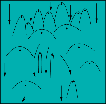
Figure 1: A schematic diagram which illustrate the main features which we might expect when a supersonic, tenuous flow encounters a region containing many discrete clouds. The clouds are not drawn to scale.

In this paper we use hydrodynamical calculations to investigate the nature of the interaction between a tenuous flow and a number of mass sources. In Section 2 we describe the problem and the basic assumptions used. The numerical results for single to multiple mass sources interacting with both a hypersonic and transonic wind are presented in Section 3. Section 4 contains our conclusions and ideas for future work.

2 The Model

As our investigation is still in its early stages, in this study we concern ourselves with only the general properties of the interaction of a wind with injected material. We do not, therefore, attempt to model the detail of how material is injected. Instead, we follow the approach in Falle et al. (2002) by assuming a uniform rate of mass injection within a given radius. This is simple to implement, but has the disadvantage that the flow from the injection region is isotropic. The mass loss from a cloud will not be isotropic if it is caused by hydrodynamic ablation by an incident wind, or by photoevaporation by radiation from a nearby star, but we show in Section 3.1.1 that the effect of asymmetrical mass loss is small at large distances from the cloud. Therefore, the actual details of the mass injection process are relatively unimportant. We also emphasize that the boundary of this injection region is not meant to be the boundary of a cloud. In fact, the cloud could be much smaller.

In this paper we are concerned with the interaction of a flow incident on several mass sources. Three dimensional calculations are required if the sources are spherical. To reduce the computational cost we restrict ourselves to two dimensional simulations where the sources are cylindrical. While we expect some differences between calculations performed in 2D and 3D, at this stage we can still gain important insight from less computationally demanding 2D simulations.

We investigate the simplest case in which the incident wind behaves adiabatically and the injected gas remains isothermal. This is motivated by the fact that if mass injection is due to photoevaporation, the injected temperature will be $\sim 10^{4}$ K, which is comparable to that of a wind whose temperature is determined by photoionization - the wind, however, can be shocked to much higher temperatures, which is the reason why we can see tails from mass sources in many astrophysical media. To ensure the above behaviour, we use an advected scalar, $\alpha$, which is unity in the injected gas and zero in the ambient gas. The source term in the energy equation is then

$$K\alpha\rho(T_{\rm 0}-T),$$ (1)

where $\rho$ and $T$ are the local mass density and temperature, and where $K$ is large enough that the temperature always remains close to the equilibrium temperature, $T_{\rm 0}$, in the injected gas. Inside the injection region we add an extra energy source so that the gas is injected with temperature unity (see Falle et al. (2002) for further details).

The calculations reported in this paper use Cobra, a 2nd order accurate code with adaptive mesh refinement (AMR). Cobra uses a hierarchy of grids $G^{0}...G^{N}$ such that the mesh spacing on grid $G^{n}$ is $\Delta x_{0}/2^{n}$. Grids $G^{0}$ and $G^{1}$ cover the whole domain, but the finer grids only exist where they are needed. The solution at each position is calculated on all grids that exist there, and the difference between these solutions is used to control refinement. In order to ensure Courant number matching at the boundaries between coarse and fine grids, the time step on grid $G^{n}$ is $\Delta t_{0}/2^{n}$ where $\Delta t_{0}$ is the time step on $G^{0}$. Such a hierarchical grid structure not only improves the efficiency by confining the fine grids to where they are needed, but it also makes it possible to use a full approximation multigrid algorithm to accelerate the convergence to the steady state (see, e.g., Brandt, 1977). Further details of Cobra can be found in Falle & Giddings (1993).

3 Results

3.1 Single and Twin Mass Sources

Our first investigations are of one and two mass sources interacting with an ambient flow. So that the ambient wind does not affect the flow in the injection region, we must ensure that the ram pressure of the injected material at the boundary of the injection region is larger than that in the wind, i.e. we require

$$a^{2}\rho_{\rm s}=\frac{ar_{\rm c}Q}{3}\geq\rho_{\rm w}v_{\rm w}^{2},$$ (2)

where $r_{\rm c}$ is the radius of the injection region, $a$ is the flow speed of injected material at $r=r_{\rm c}$ and $\rho_{\rm s}$ its density at this point, $Q$ is the mass injection rate per unit volume within $r=r_{\rm c}$, and $\rho_{\rm w}$ and $v_{\rm w}$ are the wind density and velocity (cf. Equation 5 in Falle et al. (2002)). We again emphasize that the cloud radius could actually be much smaller than $r_{\rm c}$.

3.1.1 Hypersonic wind

We choose units such that $r_{\rm c}=1$, $a=1$, $\rho_{\rm w}=1$, and set $v_{\rm w}=20$ and $T_{\rm 0}=1$, which correspond to an external isothermal Mach number of 20. Equation 2 then implies $Q\geq 800$ in order to prevent the wind from penetrating the mass injection region, although Falle et al. (2002) note that in the supersonic case a better estimate is obtained by replacing $\rho_{\rm w}v_{\rm w}^{2}$ by the pressure behind a stationary normal shock in the wind. This gives

$$Q\geq\frac{4}{\gamma+1}\frac{\rho_{\rm w}v_{\rm w}^{2}}{ar_{\rm g}}=600$$ (3)

for $\gamma=5/3$. We set $Q=700$ in order to ensure that the interaction occurs slightly outside the mass-injection region. As in Falle et al. (2002), we set the coefficient $K$ to 50, which is large enough to ensure that the temperature in the injected gas stays close to unity.

The computational domain is $0\leq x\leq 50$, $-50\leq y\leq 20$ with the mass injection region initially centered at the origin. 5 grid levels $G^{0}...G^{4}$ were used, with $G^{0}$ being $50\times 70$ and $G^{4}$ $800\times 1120$. The diameter of the mass injection region is 32 cells on the $G^{4}$ grid. Artificial dissipation is added to the simulations in order to eliminate the ‘carbuncle effect’ and to damp Kelvin-Helmholtz instabilities due to velocity shear at the contact discontinuity. This allows a steady-state solution.

Fig. 2 shows the density, pressure, and y-velocity, together with the regions occupied by the finest grid. The wind is decelerated by a bow shock, which stands off from the center of the mass source by a distance of approximately 8 units. A contact discontinuity separates the wind from the injected material. As noted in Falle et al. (2002) for the case of a spherical mass source, the injected material is not confined to a long thin tail. Instead the contact discontinuity has a half-width of $\approx 20$ at $y=-50$, which is much wider than the mass source. It is also much wider than the equivalent width observed at the same distance downstream from a spherical mass source, due to the reduced divergence in the 2D simulation. It appears that the contact discontinuity does not reach an asymptotic off-axis distance far downstream, but rather tends towards a finite opening angle (this can be further discerned in Fig. 12). Though not shown here, the opening angle is dependent on the Mach number of the wind - the injected material is more confined at lower Mach numbers, though the opening angle of the bowshock is greater. A reverse shock surrounds the mass source, and delineates the position at which the isotropic injected material feels the presence of the ambient wind.

Figure 2: Density, pressure, y-velocity, and $G^{4}$ for the simulation of a hypersonic flow interacting with a single cylindrical mass source.

In Fig. 3 we show density plots from simulations where the density, velocity, and pressure of the injected material is specified around the edge of the injection region. This approach allows us to investigate the effect of non-isotropic mass injection on the interaction with the ambient wind. In the simulation shown in the left panel of Fig. 3 we set $\rho_{\rm s}=350$ and $a=1$, and keep the other parameters as before. The total mass-injection rate is the same as that in Fig. 2, though the energy injection is slightly different. The latter means that there are slight differences between the density plots in Figs. 2 and 3. In the middle panel of Fig. 3 we keep the same overall mass injection rate, but vary the density at the edge of the injection region according to the prescription

$$\rho_{\rm s}=\rho_{0}(1-\Omega^{2}\sin^{2}\theta),$$ (4)

where $\rho_{0}$ is a normalization factor, $\theta$ is the angle between the radial vector from the injection region and the ambient flow ($\theta=\pi$ on the upstream surface, and $\theta=0$ on the downstream surface), and $\Omega$ sets the degree of anisotropy. We set $\Omega=0.9$, so that the mass injection rate at the upstream and downstream surfaces is $\approx 5\times$ that at $\theta=\pi/2$. While there are differences in the morphology of the interaction close to the injection region (e.g., the bow shock stands further off, and the shape of the reverse shock reflects the latitudinal variation of the mass and energy injection), the large scale features are remarkably unchanged. In the right panel of Fig. 3 the injection rate is highest at the upstream surface and declines smoothly towards the downstream surface, according to the prescription

$$\rho_{\rm s}=\rho_{0}[1+\Omega\sin(\theta+\pi/2)].$$ (5)

This prescription may be expected to be more representative of reality. With $\Omega=0.7$, the mass injection rate at the upstream surface is $\approx 5\times$ that at the downstream surface. Again we see that the large scale features are very similar, though as expected the bowshock stands slightly further off than in the other two cases.

Figure 3: Density plots for the simulation of a hypersonic flow interacting with a single cylindrical mass source, where the injected material is isotropic (left) and non-isotropic (middle and right). The large-scale structure is similar in all cases.

Figure 4: Density plots for the simulation of a hypersonic flow interacting with two cylindrical mass sources as a function of their separation, which increases from 12 units (top left), to 24 units (top right), to 48 units (bottom left), to 96 units (bottom right).

In Fig. 4 we show the density from calculations where the mass source is moved off-axis, which simulates the interaction of a wind with 2 identical sources. The separation between the two sources increases from 12, to 24, to 48, to 96 units. In the top left panel of Fig. 4 the two sources are surrounded by a global contact discontinuity, and not individual ones. The bow shock is located further upstream compared to that in Fig. 2, and is also global in the sense that it envelops the two mass sources, as opposed to individual shocks surrounding each source. When the mass sources are still fairly close together, the flow between them is at a higher pressure than the corresponding flow around the outside edge of the interaction. This causes the flow around each mass source to angle away from each other, and is easily identified by the tilt of the reverse shock around each source relative to the flow of the ambient wind.

As the mass sources are separated, first the global contact discontinuity splits into individual contacts around each source, and then the global bow shock separates into individual bow shocks. The reverse shock around each mass source is once again aligned with the oncoming wind, and the tail of injected material is initially symmetrical and unaffected by the presence of the other mass source. However, some interaction occurs further downstream where the bowshocks interact. At this point a reflected shock is formed, and further downstream this deflects the contact discontinuity and the tail of injected material away from the axis of symmetry. The simulations shown in Fig. 4 used 4 grid levels $G^{0}...G^{3}$. The diameter of the mass injection region is 16 cells on the $G^{3}$ grid. For the models with separations of 12, 24, and 48 units, the $G^{3}$ grid is $400\times 560$, and the computational domain is $0\leq x\leq 50$, $-50\leq y\leq 20$. The model with a separation of 96 units has a $G^{3}$ grid of $768\times 960$, and a computational domain which encompasses $0\leq x\leq 96$, $-100\leq y\leq 20$.

3.1.2 Transonic wind

In many situations it is usual for a wind to encounter a large number of mass sources. In such circumstances the Mach number of the wind is driven towards unity (Hartquist et al., 1986), and it is therefore reasonable to look at the interaction of mass sources with a transonic wind. In this case we set $r_{\rm c}=1$, $a=1$, and $T_{\rm 0}=1$ as before but now $\rho_{\rm w}=10^{-3}$, $v_{\rm w}=40.825$, giving a Mach number of unity in the undisturbed wind. Equation 2 gives $Q\geq 10/3$, which is a good estimate for this case since there is no shock upstream of the injection region. We therefore set $Q=10/3$, and the coefficient $K$ to $10^{2}$ (cf.  Falle et al., 2002).

Figure 5: The effect of the turbulence model on a calculation where a cylindrical source of mass injection interacts with a transonic wind. In the left panel we solve only the Euler equations. In the right panel we add a turbulence model where velocity shear is converted into a scalar which represents the turbulent energy density, and an additional scalar controls the dissipation rate. The resulting solution is an approximation to the mean flow, and the mixing of the injected gas with the original flow is modelled by the diffusive terms in the equations. In the left panel, the instabilities in the tail occur further upstream if the numerical resolution of the calculation is increased, since the numerical viscosity is reduced. In contrast, the turbulence model in the simulation in the right panel prevents resolution dependent instabilities.

Simulations with a transonic wind pose additional difficulties compared to the hypersonic wind case. First, in order for the boundaries to have no effect on the solution, the computational domain has to be very large, particularly since our 2D simulations have reduced divergence compared to the case of spherical mass injection regions. To satisfy this condition we find that we need $0\leq x\leq 320$, $-416\leq y\leq 256$, which would have made the calculation extremely expensive if an AMR code were not employed. Second, the velocity shear between the injected material and the wind is so extreme in the transonic case that the wind flow separates and produces a turbulent wake downstream of the interaction region. Calculations based on the Euler equations cannot adequately describe such turbulence, and the only viable option is to use a turbulence model. While there are many possibilities, we use a simple $k-\epsilon$ model as used in Falle et al. (2002).

The purpose of the subgrid turbulence model is to emulate a high Reynolds number flow. It does so by including equations for the turbulent energy density and dissipation rate and using these to calculate viscous and diffusive terms. The resulting solution should be an approximation to the mean flow. The turbulent mixing of the injected gas with the original flow due to shear instabilities is modelled by the diffusive terms in the equations. Since the turbulent viscosity computed from the subgrid model depends upon the local solution, it is not very meaningful to talk about an effective Reynolds number. For example, the turbulent viscosity is largest in shear layers and essentially vanishes in regions with little shear. The model has been calibrated by comparing the computed growth of shear layers with experiments (Dash & Wolf, 1983). The model also assumes that the real Reynolds number is very large, which is the case in astrophysical flows, and that the turbulence is fully developed. Although not entirely satisfactory, such a model gives a much more realistic result than simply using grid viscosity since in that case the size of the shear instabilities are determined by the numerical resolution. Further details can be found in Falle (1994). The effect of the turbulence model is illustrated in Fig. 5.

We use 9 levels of grid refinement for our transonic simulations, $G^{0}...G^{8}$, with $G^{0}$ being $10\times 21$ and $G^{8}$ $2560\times 5376$. The diameter of the mass injection region is 16 cells on the $G^{8}$ grid. The interaction is very different from the hypersonic case, as can be seen from Fig. 6. Instead of a bow shock there is a bow wave upstream of the mass source, whose amplitude falls off as $1/r$. A very weak tail shock occurs in the wind downstream of the mass source, and this is aligned much more parallel to the ambient flow than when the mass source is spherical (cf.  Falle et al., 2002). The injected material remains in rough pressure equilibrium with the wind, and eventually becomes confined to a tail whose width is of about the same order as the injection region.

In Fig. 7 we show the density, pressure, and y-velocity from a calculation where the mass source is moved off-axis, as we again simulate the interaction between a wind and 2 identical sources. The separation between the two sources is 48 units. We immediately see that the tail produced behind each mass source is strongly curved towards the other, producing a narrow channel between the tails. However, it is clear that the tails are initially tilted away from each other, as shown by the position of the reverse shock around the mass source. The widening of the channel between the two mass sources, which is enhanced by the curvature of the inner side of the contact discontinuity, causes the pressure within the channel to drop via the Bernoulli effect as the wind accelerates and becomes supersonic. The fall in pressure relative to that on the outside edge of the tail results in the tail curving towards the axis of symmetry, and the channel is then closed off. A shock in the channel just above this point slows the accelerated wind. There is no sign of any tail shock in the downstream wind on the outer side of the tail.

Figure 6: Density, pressure, and y-velocity for the simulation of a transonic flow interacting with a single cylindrical mass source.

Figure 7: Density, pressure, and y-velocity for a transonic flow interacting with two cylindrical mass sources separated by 48 units.

Further simulations reveal that the curvature of the tails towards each other decrease when the separation between the mass sources is increased. At large enough separations there is no interaction between the mass sources and the tails remain perfectly straight.

3.2 Multiple Sources in a Hypersonic Wind

In this section we investigate the interaction between a hypersonic flow and a group of 5 mass sources (10 with the imposed symmetry), and use the turbulence model noted in Section 3.1.2 for these calculations.

In the first simulation the sources are randomly distributed within a circular region of diameter 160 units. This diameter is increased in subsequent simulations, in order to explore differences between an interaction which is dominated by the mass injection to one which is dominated by the wind, though the relative positions of the sources remain the same. We define the parameter $\chi=\hbox{${\dot{M}}$}_{\rm c}/\hbox{${\dot{M}}$}_{\rm w}$, where $\hbox{${\dot{M}}$}_{\rm c}$ is the combined mass injection rate of the sources and $\hbox{${\dot{M}}$}_{\rm w}$ is the mass flux in the wind through a suitably chosen region. When we change the size of the region in which the mass sources are distributed, we alter the value of $\chi$ since $\rho_{\rm w}$ and $v_{\rm w}$ are kept constant. The mass injection regions have diameters of 8 cells on the finest grid in each of the models presented in this section.

The positions of the 5 sources in our first simulation are $(x,y)=(33.72,-57.12)$, (48.69,-13.70), (39.07,2.54), (24.68,55.46), and (7.89,-14.51). The best estimate for $\hbox{${\dot{M}}$}_{\rm w}$ is obtained from the evaluation of the flow rate through a region bounded by the symmetry axis and the source region whose $x$-coordinate is furthest from this. $D$ is set to the value of this $x$-coordinate. Thus $\hbox{${\dot{M}}$}_{\rm w}=\rho_{\rm w}v_{\rm w}D=20\times 1\times 48.69=973.8$. Because we are adding mass and energy to the wind, we use a slightly higher value of $Q$ in these simulations to ensure that the flow does not enter any of our source regions ($Q=880$). Therefore, $\chi=5\pi\times 880/973.8\approx 14$ and we expect the interaction to be injection-dominated. We use 5 grid levels, $G^{0}...G^{4}$ with $G^{0}$ being $40\times 60$ and $G^{4}$ $640\times 960$. The computational domain is $0\leq x\leq 160$, $-160\leq y\leq 80$.

In Fig. 8 we show the density, pressure, y-velocity, and the advected scalar of this model. A global bow shock exists around the group of mass sources and the region between the sources is filled with high pressure, low Mach number gas. The shape of the global bow shock is to some extent determined by the positions of the individual sources, and has an opening angle which is much wider than that obtained when there are only one or two sources (cf. Section 3.1.1). Downstream of the mass sources the injected material is accelerated by a pressure gradient in a manner similar to that of a superwind. The shape and position of the reverse shock around each mass source is dependent on the local flow conditions, and in some cases is almost spherical. Close up images of some of the injection regions are shown in Fig. 9. The bottom right panel of Fig. 8 reveals that the group of mass sources is largely impervious to the oncoming wind. The mass source which is furthest upstream is somewhat akin to a continental divide in the sense that it splits the wind flow to the left or right. Since we impose symmetry at $x=0$ a high pressure region of shocked ambient wind is formed - wind in this region is able to percolate through the region of mass sources, and is the only part of the oncoming flow which is able to do so.

Figure 8: Density, pressure, y-velocity, and advected scalar for the interaction of a hypersonic flow with multiple cylindrical mass sources.

Figure 9: Density images of the flow in the vicinity of three of the injection regions in the simulation shown in Fig. 8.

If the distances between the mass sources are increased by a factor of 4, $\chi$ is reduced to $\approx 3.5$. The interaction between the wind and the injected material is still dominated by the mass sources, as shown in Figs. 10 and 11, but to a lesser extent than the simulation shown in Fig. 8. The mass source furthest upstream again acts like a continental divide. However, the flow in the vicinity of this source is identical to the single source case, being unaltered by the complexities of the interaction further downstream. Specifically, the reverse shock around the mass source is not tilted or compressed. Where the interaction with $\chi\approx 14$ is characterized by a large region of subsonic flow, the interaction with $\chi\approx 3.5$ has a complex structure with multiple shocks, as is readily apparent in Fig. 10. This is due to the fact that the distances between the mass sources are such that pressure gradients in the vicinity of each source accelerate the flow to supersonic velocities before additional mass sources are encountered further downstream. In addition to a region near the axis of symmetry, the advected scalar reveals that the wind is able to force its way between the mass sources in two distinct streams, which become diluted by injected material along their length. In this simulation we used 7 grid levels, $G^{0}...G^{6}$ with $G^{0}$ being $40\times 60$ and $G^{6}$ $2560\times 3840$, spanning a computational domain of $0\leq x\leq 640$, $-640\leq y\leq 320$.

Figure 10: The density (left panel) and advected scalar (right panel) in the interaction of a hypersonic flow with multiple cylindrical mass sources when $\chi\approx 3.5$.

Figure 11: Enlargements of the regions around the 5 mass sources in the simulation shown in Fig. 10.

An increase in the separation of the mass sources by another factor of 4 reduces $\chi$ to approximately unity. We now expect the wind to begin to force its way through the region of mass sources, and this is demonstrated in Fig. 12, a simulation making use of 9 grid levels, $G^{0}...G^{8}$ with $G^{0}$ being $40\times 60$ and $G^{8}$ $10240\times 15360$ (157 million cells equivalent). The computational domain spans the region $0\leq x\leq 2560$, $-2560\leq y\leq 1280$. The distances between each mass source are now so great that there is very little interaction between them, the main difference being that the sources which are furthest downstream are interacting with a supersonic flow whose properties have been somewhat modified by the action of the sources further upstream.

Figure 12: The density (left panel) and advected scalar (middle panel) in the interaction of a hypersonic flow with multiple cylindrical mass sources when $\chi\approx 1$. An enlargement of the flow around two of the mass sources is displayed in the right panel.

The density and Mach number averaged across $x$ in the disturbed flow as a function of $y$ for each of the three simulations discussed in this section are shown in Fig. 13. The Mach number is mass averaged and not volume averaged. We see that when the rate of mass injection dominates the mass flux of the wind (i.e. $\chi\gg 1$) the average density across the width of the interaction region is very high, being of order 200 times the ambient density of the wind over a large volume of the region that contains the mass sources. The corresponding Mach number in this case is typically 0.5. The density decreases and the Mach number increases downstream of the region containing the mass sources, and the flow passes through a sonic point at roughly the same $y$-coordinate as that of the most downstream mass source. The density and Mach number profiles are fairly smooth, though there are some features with small spatial scales.

As $\chi$ decreases, the mass sources have a much more localized effect on the flow. When $\chi=3.5$, we see that the flow between the most upstream mass source (at $y\approx 222$) and its nearest companion (at $y\approx 10$) becomes supersonic, and thus knows nothing of the presence of this second source prior to the bowshock around it. The density in this part of the flow thus significantly decreases from its peak post-shock value around the first mass source ($\rho\approx 200\rho_{\rm amb}$) until its encounter with the second mass source ($\rho\approx 8\rho_{\rm amb}$ just ahead of the bowshock). There are a few places in the interaction region where the flow averaged over the width of the interaction is subsonic, and these are associated with local maxima in the corresponding density profiles. Once again, the overall flow passes through a sonic point close to the $y$-coordinate of the most downstream mass source. Compared to the simulation with $\chi=14$, the density enhancement of the mass-loaded flow is much reduced, and the averaged flow is able to maintain a higher Mach number. The trends which we have noted above continue as $\chi$ is made yet smaller. When $\chi=0.88$ the individual mass sources appear to act only as localized perturbations on the flow.

The pressure at a given radius from the centre of specific mass sources is shown in Fig. 14. In this figure we have chosen mass sources with the most uniform pressure surroundings in the two models considered. We see that the pressure around a specific mass source tends to be higher when $\chi$ is large. When the reverse shock extends to radii exceeding that at which the pressure profile is obtained, the pressure drops to a low value. In the simulation with $\chi=3.5$ we typically find that the pressure is lowest on the downstream side of the mass source, and highest on the upstream side. However, this ‘memory’ of the ambient flow is reduced as $\chi$ increases - in the top left panel of Fig. 14 we see that the maximum pressure occurs on the downstream side of the mass source. Another noteable feature is that the pressure as a function of azimuthal angle around the mass source may be fairly constant when $\chi$ is large. We anticipate that if the pressure is high and relatively uniform then there will be a greater probability that the clump could collapse and give rise to new star formation, than when the pressure is low, or varies significantly around the clump.

Although we raised the possibility of flickering in Section 1, we see little evidence for this in our models. The horizontal shock in the injected material at $y\approx-10$ in the $\chi\approx 3.5$ model (see Fig. 10 and the bottom left panel of Fig. 11) was observed to display some vertical oscillations, but these may be the result of the system relaxing to a steady state and we have not evolved the simulation long enough to eliminate this possibility. We anticipate that flickering may be more apparent in a simulation where the mass injection rate from each source responds to the local flow conditions.

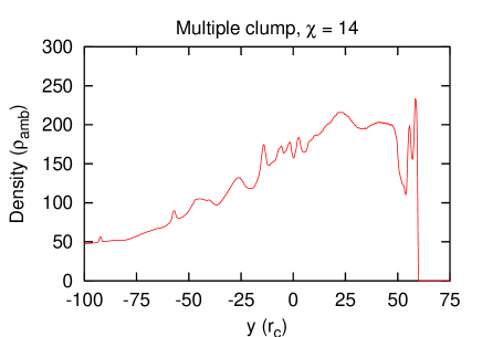
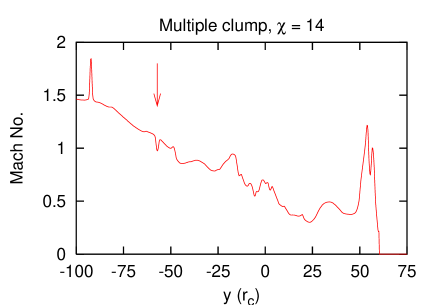
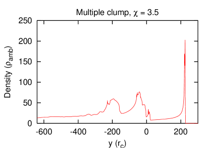
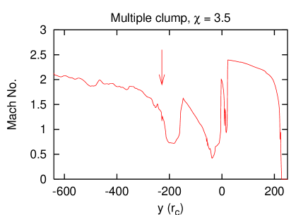
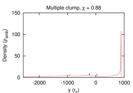
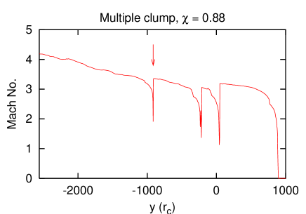
Figure 13: The density and Mach number averaged across the interaction region as a function of downstream distance for a supersonic wind impinging on a region containing many mass sources. The parameter $\chi$ describes the ability of the wind to penetrate through the region containing the mass sources. The arrows marked on the Mach number plots illustrate the $y$-coordinate of the mass source that is furthest downstream.

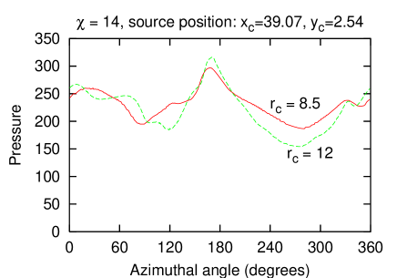
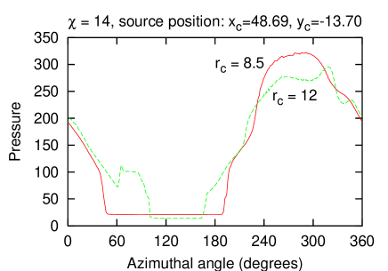
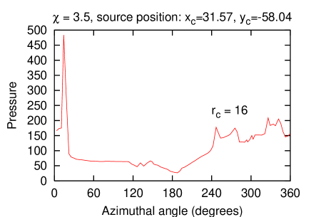
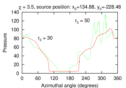
Figure 14: Pressure profiles around some of the mass sources in the simulations. In each panel the value of $\chi$ and the position of the mass source are identified. The radius at which the pressure profile was taken is noted in each panel. The azimuthal angle is $0^{\circ}$ on the upstream side of the mass source and increases clockwise.

4 Conclusions

The results shown in Section 3 illustrate that a 2D calculation of mass injection from a cylindrical source can produce flow features which are similar to those obtained in an axisymmetric simulation where mass is injected from a spherical source (cf.  Falle et al., 2002). For the interaction with a hypersonic wind, these features include the presence of a bow shock and the fact that injected material occupies a downstream region with a width significantly larger than that of the injection region. For the interaction with a transonic wind, the tail produced in the cylindrical case is slightly broader than that produced in the spherical case, but in both cases the injected material occupies a region whose width is considerably less than that obtained when the wind is hypersonic.

When two mass sources are in close proximity, their interaction may affect the shape and alignment of the tail which forms downstream of each source. Deviation in the alignment of the tails is caused by pressure differences either side of each mass source and by interaction with the reflected bow shock. These induce velocity components into the flow perpendicular to the upstream velocity of the ambient wind. A global bow shock envelops the mass sources when they are close to each other, but increasing their separation leads to an individual bow shock around each source.

For the transonic case, the curvature of the tails is also produced by pressure differences. The region between the two tails acts as a narrow channel, and the curvature of the contact discontinuity causes the wind material which travels between the tails to be accelerated. This is accompanied by a pressure drop, and the pressure differences on either side of the tail force the injected material towards the symmetry axis. In both the hypersonic and transonic cases, separating the sources reduces the degree of the interaction effects.

An interesting result is that in the hypersonic case, tails which show deviations from alignment with the upstream wind velocity are pointing away from the mass sources, whereas in the transonic case the tails end up pointing towards each other. While this could be a useful way of determining whether the wind impacting on two mass sources which are close together is hypersonic or transonic, it is possible that in a 3D model the wind between the mass sources would not be accelerated as much, leading to smaller pressure differences on either side of a tail and less significant curvature. The morphology of the tail (broad and ‘stubby’, versus long and thin) is instead a much simpler way to determine the nature of the interaction.

With multiple mass sources in a hypersonic flow, the ability of the wind to punch through the space between the sources depends on the ratio of the mass injection rate from the sources to the mass flux in the wind, which we have called $\chi$. When $\chi$ is much greater than unity, the sources are an effective barrier, and allow very little of the impacting wind to find a path through them. A global bowshock exists around the sources and the space between the sources is filled with a high pressure, subsonic flow of injected material. When $\chi$ is less than or of order unity, the wind is able to force its way inbetween the mass sources, and for the most part this flow is much less pressurized and highly supersonic. We see little evidence for flickering in our current models.

In future work we will consider 3D simulations, different treatments of cooling, and the response of the mass injection rate of each source to the local flow conditions. We will also apply these results to specific objects (e.g., planetary nebulae).

References

- Brandt (1977) Brandt A., 1977, Math. Comput., 31, 333
- Dash & Wolf (1983) Dash S. M., Wolf D. E., 1983, AIAA paper 83-0704
- Dyson (2003) Dyson J. E., 2003, Ap&SS, 285, 709
- Dyson, Hartquist & Biro (1993) Dyson J. E., Hartquist T. W., Biro S., 1993, MNRAS, 261, 430
- Falle (1994) Falle S. A. E. G., 1994, MNRAS, 269, 607
- Falle & Giddings (1993) Falle S. A. E. G., Giddings J. R., 1993, in Morton K. W., Baines M. J., eds., Numerical Methods for Fluid Dynamics 4. Clarendon Press, Oxford, p. 335
- Falle et al. (2002) Falle S. A. E. G., Coker R. F., Pittard J. M., Dyson J. E., Hartquist T. W., 2002, MNRAS, 329, 670
- Falle, Komissarov & Joarder (1998) Falle S. A. E. G., Komissarov S. S., Joarder P., 1998, MNRAS, 297, 265
- Gregori et al. (2000) Gregori G., Miniati F., Ryu D., Jones T. W., 2000, ApJ, 543, 775
- Hartquist et al. (1986) Hartquist T. W., Dyson J. E., Pettini M., Smith L. J., 1986, MNRAS, 221, 715
- Jun, Jones & Norman (1996) Jun B.-I., Jones T. W., Norman M. L., 1996, ApJ, 468, L59
- Klein et al. (2003) Klein R. I., Budil K. S., Perry T. S., Bach D. R., 2003, ApJ, 583, 245
- Klein, McKee & Colella (1994) Klein R. I., McKee C. F., Colella P., 1994, ApJ, 420, 213
- Lim, Hartquist & Williams (2001) Lim A. J., Hartquist T. W., Williams D. A., 2001, MNRAS, 326, 1110
- Mac Low et al. (1994) Mac Low M.-M., McKee C. F., Klein R. I., Stone J. M., Norman M. L., 1994, ApJ, 433, 757
- Poludnenko et al. (2004) Poludnenko A. Y., Dannenberg K. K., Drake R. P., Frank A., Knauer J., Meyerhofer D. D., Furnish M., Asay J. R., Mitran S., 2004, ApJ, 604, 213
- Poludnenko, Frank & Blackman (2002) Poludnenko A. Y., Frank A., Blackman E. G., 2002, ApJ, 576, 832
- Quik (1994) Quik J. J., 1994, Int. J. Numer. Meth. Fluids, 18, 555
- Xu & Stone (1995) Xu J., Stone J. M., 1995, ApJ, 454, 172