Radiative Transfer and Acceleration in Magnetocentrifugal Winds

Abstract

Detailed photoionization and radiative acceleration of self-similar magnetocentrifugal accretion disk winds are explored. First, a general-purpose hybrid magnetocentrifugal and radiatively-driven wind model is defined. Solutions are then examined to determine how radiative acceleration modifies magnetocentrifugal winds and how those winds can influence radiative driving in Active Galactic Nuclei (AGNs). For the models studied here, both radiative acceleration by bound-free (“continuum-driving”) and bound-bound (“line-driving”) processes are found to be important, although magnetic driving dominates the mass outflow rate for the Eddington ratios studied ($L/L_{\rm Edd}=0.001-0.1$). The solutions show that shielding by a magnetocentrifugal wind can increase the efficiency of a radiatively-driven wind, and also that, within a magnetocentrifugal wind, radiative acceleration is sensitive to both the column in the shield, the column of the wind and the initial density at the base of the wind.

1. Introduction

A variety of observational signatures point to the importance of outflowing gas within many types of Active Galactic Nuclei (AGNs). Blueshifted absorption features (in Broad Absorption Line Quasars, or BALQSOs; see, e.g., Weymann et al., 1991) are seen in approximately 15% (Reichard et al., 2003) of radio-quiet quasars, with velocities up to 0.1c. In addition, radio-loud quasars display relativistic, collimated outflows. More recently, both UV and X-ray absorbing gas have been observed in approximately 60% of Seyfert 1 galaxies (Crenshaw et al., 1999). Observational estimates hint that the mass outflow rate is nearly equal to the mass inflow rate (for a review of mass outflow in AGNs, see Crenshaw, Kraemer, & George, 2003).

The development of models to explain the mass outflow rates, geometry, and general kinematics of these winds has proven difficult, but progress on a number of possibilities has been encouraging. From very early on, researchers examined both radiative wind models (e.g., Drew & Boksenberg, 1984; Vitello & Shlosman, 1988) and, to explain radio jets, hydromagnetic models (e.g., Blandford & Payne, 1982, hereafter BP82). Later models of radiatively-driven winds were able to explain the BALQSO outflow velocities and population fraction (Murray et al., 1995, hereafter, MCGV95) as well as the single-peaked emission lines (Murray & Chiang, 1997). The line-driven models were also demonstrated in hydrodynamical simulations (Proga, Stone & Drew, 1998; Proga, Stone, & Kallman, 2000; Pereyra et al., 2004), which elucidated the density structure, geometry, and kinematics of the flow in two dimensions. In addition, models with combinations of continuum- and line-driving by X-rays were presented by Chelouche & Netzer (2001). One of the concerns with line-driving in AGNs has been the possible over-ionization of the gas by X-rays in the central continuum (leaving the wind with too few lines to intercept flux in the lines): the need for “shielding gas” to prevent this overionization has been a persistent concern (e.g., MCGV95, Chelouche & Netzer, 2003b; Proga & Kallman, 2004).

In addition, hydromagnetic winds have also been developed to gain insight into the observations; some of these models have included radiative driving. In these magnetocentrifugal winds, gas is loaded onto and tied to large-scale magnetic field lines; those field lines then fling the matter centrifugally away from the disk, like beads along a wire. Magnetocentrifugal acceleration is commonly used to explain large-scale collimated outflows in radio galaxies (BP82; for reviews of magnetocentrifugal driving, see Spruit, 1996; Königl & Pudritz, 2000; Ferreira, 2003). In the context of the Broad Emission Line Region (BLR), magnetocentrifugal outflows made up of clouds were first called upon to explain the single-peaked broad emission lines, outflow velocities, and densities (Emmering et al., 1992) . The “torus” (obscuring gas that plays a central role in the Unification model, yielding a dependence of observed properties with inclination angle; see Antonucci, 1993) has been explained as a dusty, continuous magnetic wind (Königl & Kartje, 1994, hereafter KK94) where radiative acceleration on dust affects the wind geometry. Hydromagnetic disk winds with radiation pressure were also developed by de Kool & Begelman (1995) as an alternative explanation for the population fraction of BALQSOs and to understand cloud confinement within the outflow. In addition, another magnetocentrifugal wind model was developed to explain single peaked emission lines arising from a distribution of clouds (Bottorff et al., 1997), as well as the dynamics of the warm absorber in NGC 5548 (Bottorff, Korista, & Shlosman, 2000). Finally, some effects of magnetic fields (not including magnetocentrifugal driving as in BP82) have also been considered in two-dimensional hydrodynamic simulations (Proga, 2000, 2003).

At the present time, both radiatively driven winds and magnetocentrifugally driven winds (with radiative acceleration added in some models) offer compelling but competing pictures of the key physics in the cores of AGNs. No clear observational evidence yet discriminates the dominant physics of wind-launching in AGNs. For radiatively-driven winds, three main lines of evidence hint that radiative driving should be important in models of wind dynamics. First, Laor & Brandt (2002) find a correlation between UV luminosity and the observed outflow velocity, which agrees with a basic prediction of line-driven wind models (Proga, 1999). In addition, the “ghost of Ly-$\alpha$” (Arav et al., 1995; Chelouche & Netzer, 2003b), as well as the realization that the radiative momentum removed from the continuum in blueshifted absorption lines in BALQSOs is a significant fraction of the total radiative momentum (MCGV95) are both also important clues that radiative acceleration is an important component to any self-consistent model of AGN winds. There are still, however, concerns about how the “shielding” of the wind works (Chelouche & Netzer, 2003b; Proga & Kallman, 2004). In addition, in the case of stellar disk winds, observations of two nova-like variables seem to show that their winds are not dominated by radiative driving (Hartley et al., 2002). (This conclusion, however, rests on the prediction that line equivalent widths are direct measures of mass outflow rate, which may not be the case; see Pereyra et al., 2004)

On the other hand, the leading model for collimated radio jets in AGNs (BP82) already calls upon large scale, dynamically important magnetic fields, as do the hydromagnetic wind models (mentioned above, e.g. Königl & Kartje, 1994; Kartje, 1995; Bottorff et al., 1997) that have also had success in explaining AGN observations. In addition, such a hydromagnetic wind would have no difficulty with overionization, and so might naturally serve as a “shield” for radiative acceleration further from the central source. There are, however, currently no models which address the interplay between magnetocentrifugal driving and radiative acceleration; if such wind models could be constrained, we may be able to observationally distinguish the physics of wind launching in the cores of AGNs, and gain insight into the role that outflows play both in accretion and in feedback of those winds in the galaxy and surrounding matter.

This paper develops a detailed photoionization and dynamical model for magnetocentrifugal winds in AGNs. The model is designed to explore the radiative transfer within such magnetocentrifugal winds, but also to help understand how radiative driving impacts the kinematic structure of such winds. Constructing such a model builds the foundation for later work to determine absorption and emission line profiles in order to compare with observations and check for the presence of magnetocentrifugal winds within AGNs. An overview of this model is presented in §2; the model is then defined in detail in §3. An examination of the structure of a particular “fiducial” magnetocentrifugal, radiatively-accelerated wind is described in §4 and then the dependences of radiative acceleration on some initial parameters are shown in §5. Conclusions and directions for future work are summarized in §6.

2. Model Overview

Before examining the model in detail, it is instructive to present a summary of the basic design. The semianalytic model developed here includes magnetic acceleration and radiative acceleration of a continuous wind launched from an accretion disk. A detailed treatment of radiative transfer is included by using Version 96.00 of the photoionization simulation program Cloudy, last described by Ferland et al. (1998). These elements are introduced in an approximate schematic of the wind model shown in Figure 1, depicting a portion of the accretion disk and outflowing wind. In this figure, radiation (entering from the left side of the schematic) first encounters a purely magnetocentrifugally accelerated wind, which will be referred to as the “shield”, as it absorbs radiation from the central continuum. The shield is introduced as a separate component in order to cleanly differentiate the effect of shielding from radiative acceleration; radiative driving of the shield is therefore not considered in this work. Beyond that shield is an optically thin, radiatively and magnetically accelerated wind streamline (which we will henceforth refer to as the “wind”). In this portion of the model, both magnetocentrifugal and radiative forces help accelerate the flow off of the accretion disk; the magnetic fieldlines are shown by the black lines bordering the outflow. The included radiative acceleration is calculated by first simulating the photoionization within both the shield and the wind along radial paths such as the thick, black lines in the figure.

The separation of the wind into two components is, of course, artificial. In reality, radiative acceleration would gradually increase in importance for portions of the wind that are increasingly shielded. However, splitting the outflow into these two components allows a first-order, qualitative solution that can be used to gain some understanding of how magnetic and radiative forces might interact, and how a magnetic wind may be able to act as a radiative “shield” to allow more efficient radiative acceleration. While artificial, this method of using two wind components has already been used successfully to examine winds with magnetocentrifugal and radiative driving on dust (e.g., KK94, Kartje, 1995).

Figure 2 presents a schematic flow chart of how model calculations proceed. The wind starts as a self-similar magnetohydrodynamic model that yields the pure magnetocentrifugal wind solution (covered in §3.1). Next, simulations of the photoionization balance of that wind streamline (§3.2) are run, and the resultant ionization balance and transmitted continuum are used to calculate the radiative acceleration behind the shield (§3.3). Next, the radiative acceleration is input (as a function of polar angle, $\theta$) back into the self-similar magnetohydrodynamic model, modifying the structure of the wind streamline, while leaving the shield unaffected. This process is then repeated, simulating the photoionization of that modified wind and recalculating the radiative acceleration terms. We typically iterate five to eight times to converge to a final equilibrium solution.

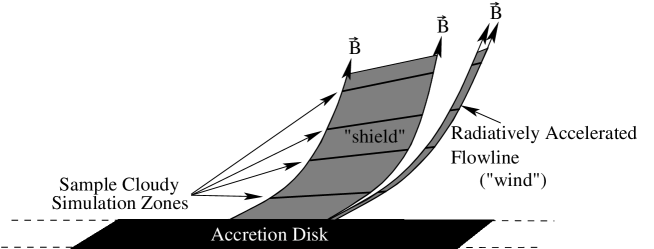
Figure 1.— Schematic of the basic geometry and major components of the radiatively accelerated magnetocentrifugal wind model. The wind itself is split into two components: a pure magnetocentrifugal wind that acts as a shield (the wider component on the left) and an optically thin streamline with combined magnetocentrifugal and radiative acceleration. The heavy black lines indicate a few of the radial zones where Cloudy simulates the photoionization balance of the wind (typically, $\sim$ 40 such radial Cloudy simulations are run, spaced logarithmically in polar angle, $\theta$).

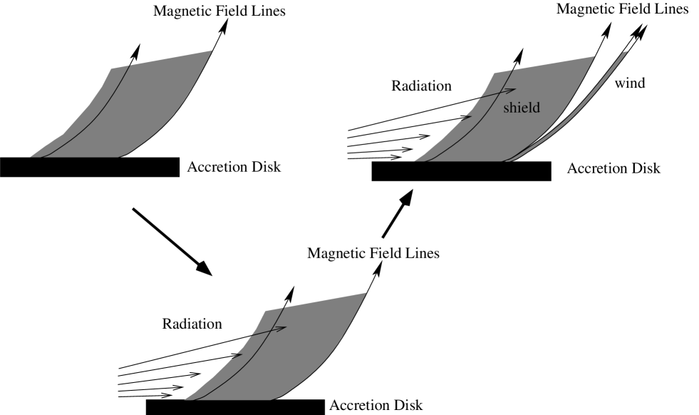
Figure 2.— The iterative scheme in the wind model, showing a single iteration of the model, moving counterclockwise around the figure. The model starts by solving the self-similar magnetohydrodynamic (MHD) equations for the structure of a centrifugally driven outflow (upper left). Next, photoionization simulations determine the continuum incident on the radiatively accelerated streamline as well as the ionization state of the gas in the streamline, and then those results are utilized to calculate the radiative acceleration of that flow. The radiative acceleration is then applied (as a function of the polar angle $\theta$) to the second component of the self-similar magnetocentrifugal wind. A new wind structure for that second section of the outflow is then derived from the interaction of those forces (upper right).

With the basic model now summarized, it may be instructive to compare and contrast it to the recent wind model examined in Proga (2003), where the combination of magnetic and radiative forces in disk winds is also investigated. Proga (2003) concentrates on numerical simulations of time-dependent winds with line driving and magnetic forces. These numerical simulations allow large-scale models of outflows that are valuable in understanding global wind structures in many different astrophysical contexts. In contrast, the radiatively-driven components of this model are more localized, since radiative acceleration is applied to the shielded streamline only. This model setup has been chosen for its flexibility in radiative acceleration modeling; using Cloudy for such radiative acceleration models enables computations not only of radiative line driving but also of continuum driving, and allows us the freedom to include dust and easily vary the incident spectrum, for example. In addition, the magnetic winds produced in Proga (2003) are not magnetocentrifugal outflows (as in BP82), as are the semianalytic winds presented here. Further, these new models are steady-state, not time-dependent. Finally, semi-analytic, steady-state models allow an exploration of general behaviors through many parameter variations; large-scale numerical simulations can usually vary only a few parameters. In summary, these models cover different facets of the disk-wind problem, yielding different perspectives on a complicated system.

3. The Two-Phase Hydromagnetic and Radiative Wind Model

In this section, we describe in detail the model’s components, and derive key equations. The magnetocentrifugal wind model is introduced first (§3.1), followed by the photoionization simulations (§3.2), radiative acceleration calculation (§3.3), and finally a discussion of the wind model equation of motion (§3.4).

3.1. Magnetocentrifugal Self-Similar Wind Solution

To derive the equations governing the continuous magnetocentrifugal wind, we start with the equations of a stationary, axisymmetric magnetohydrodynamic (MHD) flow in cylindrical coordinates, make the assumption of self-similarity in the spherical radial coordinate, and utilize the continuity equation, conservation of angular momentum along the flow, and both the radial and vertical momentum equations, very much as in BP82 and KK94 (see Appendix A). Thermal effects are neglected in the wind, therefore effectively assuming that the wind starts out supersonic (this assumption is checked later on, see §3.5). In deriving the wind equations, we use the same simplifications as BP82, except for the added complication that energy is not conserved in the radiatively-accelerated system due to the constant input of radiative energy into the wind. In the original formulation of BP82, conservation of energy supplied an additional constraint which allowed a simplification of the equations of motion to two first-order differential equations. Because energy is not conserved in this flow, the equivalent of three first-order differential equations must be integrated, solving for three parameters simultaneously instead of two as in BP82. The detailed setup and derivation of this set of equations of motion are given in Appendix A.

The integration of the momentum equations starts by specifying the following initial parameters: the mass loading of the wind (the ratio of mass flux to magnetic flux in the magnetocentrifugal wind, $\kappa\propto\frac{4\pi\rho v_{p}}{B_{p}}$, where $\rho$ is the mass density of the wind, $v_{p}$ is the poloidal velocity of the wind ($v_{p}~{}\equiv~{}(v_{r}^{2}+v_{z}^{2})^{1/2}$), and $B_{p}$ is the poloidal magnetic field strength), the specific angular momentum of gas and field in the wind, and the power-law exponent ($b$) that describes the change in density with spherical radius: $\rho\propto R^{-b}$. Also input, as parameters, are the mass of the central black hole, $M_{\bullet}$, the wind’s launch radius on the disk, $r_{0}$, and the density at the base of the wind at the launch radius, $n_{0}$. The program employs a “shooting” algorithm (using the SLATEC routine DNSQ; Powell, 1970) to integrate from the singular point (the Alfvén point) to the disk, solving for the height of the singular point above the disk ($\chi_{A}$) and the slope of the streamline at both the disk and the Alfvén point ($\xi^{\prime}_{0}$ and $\xi^{\prime}_{A}$) by matching the integration results to boundary conditions on the disk. After solving for the position of the Alfvén point, the equations of motion are integrated from the disk to a user-specified height beyond the Alfvén point; along the streamline, the run of velocity, density, and magnetic field are calculated.

This code has been tested (without radiative acceleration) against the solution given in BP82 and have duplicated their results to within 8%. This is close to the previously reported 4% variance in the recalculation of BP82 reported in Safier (1993). The difference in these new results comes not only from using higher precision calculations compared to BP82 (we use the same precision as Safier, 1993), but in addition, a more complex set of equations is being solved.

3.2. Photoionization Simulations of the Wind

Next, Version 96.00 of the photoionization code Cloudy (Ferland et al., 1998) is used to simulate the absorption of the magnetocentrifugal shield and wind as well as the ionization state at the wind streamline. Photoionization simulations of the shield and wind are used to calculate the radiative acceleration and allow considerable flexibility in gas parameters (such as gas abundances, dust, central continuum, etc). This flexibility is gained at the cost of simulating the photoionization state of the wind as if it were a static medium, as Cloudy assumes; this is only true of the recombination timescale for the gas is much shorter than the transit timescale of gas in the region simulated ($\tau_{\rm recomb}<\tau_{\rm flow}$). We have however, verified, a posteriori, that $\tau_{\rm recomb}<\tau_{\rm flow}$ for all of the radiatively accelerated ions at the base of the wind where radiative acceleration is important, using the recombination rate approximations in Arnaud & Raymond (1992) and Verner & Ferland (1996) to calculate the recombination times. Even at high latitude, $\tau_{\rm recomb}<\tau_{\rm flow}$ for all of the significant ions. At the highest latitudes, highly ionized O, which has the longest recombination time among the significantly radiatively accelerated ions, has a recombination timescale that is still a factor of two less than the transit time. Meanwhile, highly ionized Fe ions, which dominate the low level of radiative acceleration at high latitudes, have recombination timescales an order of magnitude less than the transit timescale. Using Cloudy is therefore a reasonable approximation for the radiative equilibrium within our winds (especially since, with our code, adiabatic and advective effects are added, see §3.2.1). As Cloudy enables a flexible, self-consistent calculation of radiative acceleration, we accept this approximation to enable these calculations.

Of basic importance to the photoionization simulations is the illuminating spectral energy distribution (SED). For the purposes of these simulations, an SED adapted from Risaliti & Elvis (2004) is used (an example of the SED is shown in Figure 6). This SED is input into Cloudy via the generic “AGN” continuum with $T_{\rm blackbody}=1.5\times 10^{5}$ K, $\alpha_{\rm ox}=-1.43$ (Elvis, Risaliti, & Zamorani, 2002), $\alpha_{\rm UV}=-0.44$, and $\alpha_{X}=0.9$ ($\alpha_{\rm ox}$ defines a single power-law that would describe the continuum between $2500$ Å and 2 keV, $\alpha_{\rm UV}$ is the slope of the low-energy component of the Big Blue Bump, and $\alpha_{\rm X}$ is the X-ray power-law exponent; our value of $\alpha_{\rm ox}$ is taken from the middle of the range 0.8 to 1.0 given in Risaliti & Elvis (2004)).

Spectral signatures and radiative acceleration also depend, of course, on the column density in the wind. Observations yield only rough constraints for this, so these columns as left as free parameters; the effect of varying these columns will be investigated in this paper. The columns throughout the shield and wind are set by the columns at the base of the shield and wind, denoted $N_{\rm H,0}$ for the hydrogen column at the base of the wind. As the wind rises above the disk and accelerates, that column density ($N_{\rm H}$) drops as a function of height due to mass conservation (an example of this is shown later in Fig. 7). Investigating the shielding ability of such a dynamic shielding column is of central interest to this paper, and will be addressed in §5.1.

3.2.1 Photoionization of the Continuous Wind

As depicted in Figure 1, Cloudy simulates the photoionization of the wind along radial sight lines through the shield and through the wind, ending at the site of radiative acceleration on the wind streamline. The continuum incident on the wind streamline is also calculated. The photoionization state and continuum at the end of the Cloudy calculations are recorded, and then used to compute the radiative acceleration of that gas. Finally, the acceleration is tabulated and applied as a function of $\theta$ along the wind streamline by inputing the angle-dependent radiative acceleration into the gravitational term (this is covered in more detail in Appendix A, see eqn. A3).

Whereas Cloudy is designed to simulate the photoionization balance of gases as in the shield and wind, it cannot easily incorporate adiabatic and advection effects: Cloudy has no knowledge of the particular velocity profile of the wind in the overarching model, or the temperature difference between successive photoionization models as the wind climbs above the disk. Therefore, this model calculates both advective heating and adiabatic cooling in the wind, and adds those terms manually into Cloudy’s simulations. Both terms largely cancel in the wind, and have only a negligible effect on outflow dynamics, but they are included in all of the models for completeness.

3.3. Radiative Acceleration Calculations

The model then incorporates the above-mentioned results for the ionization structure and radiation field to calculate the radiative forces felt by the wind. There are two different kinds of radiative acceleration to consider: continuum acceleration (including radiative acceleration on dust) and line acceleration. It is convenient to express the radiative acceleration in terms of $\Gamma(\theta)$,

$$\Gamma(\theta) \equiv \frac{a_{\rm radiative}(\theta)}{g},$$ (1)

where $a_{\rm radiative}$ is the acceleration due to radiation, and $g$ is the local gravitational acceleration.

3.3.1 Line and Continuum Acceleration

In general, for continuum and line acceleration, the radiative acceleration is given by

$$\Gamma = \frac{\frac{n_{e}\sigma_{T}F}{\rho c}(M_{\rm cont}+M_{\rm lines})}{\frac{GM_{\bullet}}{r^{2}+z^{2}}},$$ (2)

where $F$ is the local flux (the flux transmitted through both the shield and wind column), $n_{e}$ is the electron density, $\rho$ is the gas density, $c$ is the speed of light, $G$ is the gravitational constant, $M_{\bullet}$ is the mass of the central black hole, $r$ and $z$ are cylindrical coordinates centered on the black hole, and $M_{\rm cont}$ & $M_{\rm lines}$ are the “force multipliers” that relate how much the radiative forces on the gas (on the line and continuum opacity, respectively) exceed the radiative forces on electrons alone. They are given below in terms of the continuum opacity, $\chi_{\nu}$, and the line opacity, $\chi_{l}$, for the continuum and lines, respectively:

$$M_{\rm cont} = \frac{1}{n_{e}\sigma_{T}F}\int\chi_{\nu}F_{\nu}d\nu,$$ (3)

$$M_{\rm lines} = \frac{1}{F}\sum_{l}F_{l}\Delta\nu_{l}\frac{1-e^{-\eta_{l}t}}{t},$$ (4)

with

$$\eta_{l}\equiv\frac{\chi_{l}}{\sigma_{T}n_{e}}\hskip 72.26999ptt\equiv\frac{\sigma_{T}n_{e}v_{\rm th}}{dv_{R}/dR},$$ (5)

where $\nu$ is the photon frequency, $F_{l}$ is the local (transmitted) flux in the line at the frequency of line number $l$, $v_{\rm th}$ is the sound speed in the gas, $\Delta\nu_{l}=\nu v_{\rm th}/c$ is the thermal line width, and $\eta_{l}$ compares the opacity of the line (for a given ionization state of the gas) to the electron opacity, representing all of the atomic physics in the radiative acceleration calculation. The last remaining variable, $t$, is often called the “effective electron optical depth” and encodes the dynamical information of the wind in the radiative acceleration calculation. This dynamical information is important because in an accelerating medium, one must also account for the Doppler shift of the atomic line absorption energy in the accelerating gas relative to the emitted line photon’s energy: beyond the Sobolev length, $v_{\rm th}/(dv_{R}/dR)$, included in $t$, a line photon will be Doppler-shifted out of the thermal width of the absorption line and can escape the gas (see Sobolev, 1958; Castor, Abbott, & Klein, 1975; Mihalas & Weibel-Mihalas, 1999).

The above-mentioned force multipliers are calculated using the resonance line data of Verner et al. (1996) with solar abundances. Since $M_{\rm cont}$, the continuum multiplier, depends only on the ionization state, it is tabulated solely as a function of height in the wind. In contrast to $M_{\rm cont}$, the line multiplier ($M_{\rm line}$) is tabulated for a range of values of the parameter $t$. Later, when calculating the equation of motion for the wind, the local velocity gradient is used to compute the actual value of $t$, which is then used to linearly interpolate the table of $M_{\rm line}$ and then evaluate the radiative acceleration.

The force multiplier computation has been tested against Arav et al. (1994), who also calculated radiative acceleration from photoionization simulations. Figure 3 compares these new calculations results against their fits (noting that there is a typo in their eq. [2.9]; Z.-Y. Li, personal communication), where the force multipliers as a function of the ionization parameter $U$ is presented ($U$ is the ratio of hydrogen-ionizing photon density to hydrogen number density $n$, given by $U\equiv Q/4{\pi}nR^{2}c$, where $Q$ is the number of incident hydrogen-ionizing photons per second, and $R$ is the distance from the continuum source). Overall, good agreement is found, especially considering that Arav et al. (1994) point out that their fit deviates from their calculations at low values of $U$. The increase in the newly-calculated continuum force multiplier over Arav et al. (1994) is most likely due to the different continuum opacity database included in Cloudy 96 compared to the code (MAPPINGS) that was used in Arav et al. (1994). The multiplier values and trends with ionization parameter are still clearly very similar, however.

Figure 3.— Comparison between the force multiplier calculation in this code (solid lines) and the fits of Arav et al. (1994, dashed lines). The plot in the upper left is the comparison of the continuum force multiplier, as a function of the ionization parameter, $U$. The next three panels show a comparison of the line force multiplier (which is also a function of $t$, besides $U$) as a function of $U$ for three different values of $t$, given at the top of each panel.

3.3.2 Non-Sobolev Effects

Simply using the Sobolev length, $v_{\rm th}/(dv_{R}/dR)$, in Equation 4 can be misleading. In early simulations, we found that this Sobolev length could, in regions where the gas is slowly accelerating, be much larger than the physical size of the shield and wind combined. This is clearly not physical, so a simple non-Sobolev method was employed to calculate the size of the combined shield and wind column.

First, for the wind, the length of the absorbing column is simply limited to the minimum of the wind’s Sobolev length and its true (physical) length.

Second, for the shield, the length of the absorbing column is given by the minimum of the shield’s Sobolev length, its true physical length, and the average length of the column that absorbs photons at the wavelength of the dominant accelerating atomic lines. This last length-scale requires more explanation. To calculate this length, the top 20 line force multipliers (for individual atomic lines) are found for each polar angle $\theta$, and for each of those lines, the column of each particular ion in the shield is read from the Cloudy simulations. An average shielding column for all of the high-opacity lines is then calculated. To test this approximation, we have used lists of the top 10, 20, and 50 transitions in the wind and used them to calculate the limiting column in the shield. Changing the number of lines included does not significantly change the final wind solutions, especially since this effect is only important at the extreme base of the wind. Without considering all of these constraints on the size of the absorbing column, the Sobolev length can significantly overestimate the optical depth in the shield (even overestimating the physical length of the columns, for small accelerations), which results in the line driving acceleration dropping below the continuum acceleration. Other non-Sobolev effects (such as line blanketing within the shielding gas or the wind) are not considered in this model; for a consideration of these effects, see Chelouche & Netzer (2003a).

With a length-scale found from the sum of the wind and shield lengths found above, that length-scale is then substituted for the Sobolev length in the calculation of $M_{\rm lines}$ in Eq. 4. Including this physical length of the wind and shield will introduce dependences on the sizes of the wind and shield columns, which will be examined in §5.

3.4. Integrating the Euler Equation for the Wind

Given the results from the ionization and radiative acceleration calculations, the next step is to solve for the effect of radiative acceleration on the wind, taking the magnetocentrifugal wind model already computed and augmenting its acceleration with radiative forces. To do this, the full equation of motion (the Euler equation) is integrated along the streamline of the self-similar wind solution, recording $\Gamma(\theta)$, the radiative acceleration. $\Gamma(\theta)$ is then input into the self-similar model in the subsequent iteration (see Appendix A; specifically, eqn. A3).

In its simplest form, Euler’s Equation is given by

$$\rho\left(\frac{\partial\mathbf{v}}{\partial t}+(\mathbf{v}\cdot\nabla)\mathbf{v}\right)=\sum\mathbf{F}_{i},$$ (6)

where the $\mathbf{F}_{i}$ represent the various forces included.

As we are interested in steady-state winds, $\frac{\partial\mathbf{v}}{\partial t}$ in Eq. 6 is set to zero. As already mentioned, gravitational, radiation, and Lorentz forces are included, while thermal terms are not. This yields the expression below, with the magnetic force term is split into pressure and tension components.

$$\rho(\mathbf{v}\cdot\nabla)\mathbf{v} = -[1-\Gamma(\theta)]\frac{GM\rho}{R^{2}}\hat{R}-\frac{1}{8\pi}\nabla B^{2}+\frac{1}{4\pi}(\mathbf{B}\cdot\nabla)\mathbf{B}$$ (7)

For these calculations, it is more intuitive to integrate the equation of motion along the flow already given by the magnetocentrifugal wind solution. Therefore, taking the dot product of Euler’s equation with $\hat{s}$, which is defined as the direction along the flow, and expanding and simplifying the left-hand side of the equation, one finds:

$$(\mathbf{v}\cdot\nabla\mathbf{v})\cdot\hat{s} = v_{p}\frac{\partial v_{p}}{\partial s}-\frac{v_{\phi}^{2}}{r}\sin\theta_{F},$$ (8)

where

$$\theta_{F} \equiv \tan^{-1}\left(\frac{dr}{dz}\right).$$ (9)

In the same way, if $\theta$ is defined via

$$\theta\equiv\tan^{-1}\left(\frac{r}{z}\right),$$ (10)

the gravitational term can be written as

$$-[1-\Gamma(\theta)]\frac{GM}{R^{2}}\hat{R}\cdot\hat{s} = -[1-\Gamma(\theta)]\frac{GM}{r^{2}+z^{2}}\cos(\theta-\theta_{F}).$$ (11)

Next, we take the dot product of $\hat{s}$ with the magnetic terms to find

$$\left[-\frac{1}{8\pi\rho}\nabla B^{2}+\frac{1}{4\pi\rho}(\mathbf{B}\cdot\nabla)\mathbf{B}\right]\cdot\hat{s} = -\frac{B_{\phi}}{4\pi\rho r}\frac{\partial(rB_{\phi})}{\partial s}.$$ (12)

Combining all of those terms, the full Euler Equation is obtained:

$$v_{p}\frac{\partial v_{p}}{\partial s}-\frac{v_{\phi}^{2}}{r}\sin\theta_{F} = -[1-\Gamma(\theta)]\frac{GM}{(r^{2}+z^{2})}\cos(\theta-\theta_{F})$$ (13)

$$-\frac{B_{\phi}}{4\pi\rho r}\frac{\partial(rB_{\phi})}{\partial s}.$$

This equation is still dependent on $v_{\phi}$, however, which can be eliminated by appealing to the induction equation and $E_{\phi}=0$ for such axisymmetric systems (see, e.g., Königl & Pudritz, 2000), to yield a relation between $v_{p}$ and $v_{\phi}$:

$$v_{\phi} = \frac{v_{p}B_{\phi}}{B_{p}}+\Omega r.$$ (14)

Substituting this expression into the Euler Equation yields:

$$v_{p}\frac{\partial v_{p}}{\partial s}-\left(\frac{v_{p}B_{\phi}}{B_{p}}+\Omega r\right)^{2}\frac{\sin\theta_{F}}{r}=$$ (15)

$$-[1-\Gamma(\theta)]\frac{GM}{(r^{2}+z^{2})}\cos(\theta-\theta_{F})-\frac{B_{\phi}}{4\pi\rho r}\frac{\partial(rB_{\phi})}{\partial s}.$$

To evaluate the effective optical depth $t$, an expression is required for $dv_{R}/dR$, the spherical radial gradient of the spherical radial velocity. Since the code integrates quantities only parallel to the flow, approximations to the perpendicular velocity gradients must be used. Assuming that the derivatives of $\theta$ and $\theta_{F}$ with distance along the streamline are small (verified a posteriori to be true):

$$\frac{dv_{R}}{dR} = \hat{R}\cdot\nabla v_{R},$$ (16)

$$= \hat{R}\cdot\nabla[v_{p}\cos(\theta-\theta_{F})],$$ (17)

$$\approx \cos(\theta-\theta_{F})\left(\frac{dv_{p}}{dr}\sin\theta+\frac{dv_{p}}{dz}\cos\theta\right),$$ (18)

$$\approx \cos(\theta-\theta_{F})\frac{dv_{p}}{ds}(\sin\theta_{F}\sin\theta+\cos\theta_{F}\cos\theta),$$ (19)

$$= \cos^{2}(\theta-\theta_{F})\frac{dv_{p}}{ds}.$$ (20)

This integration procedure has been tested with radiative acceleration turned off, where it reproduces the original self-similar velocity profile to within one part in $10^{5}$. With the radiative acceleration turned on, the entire code has repeatedly converged within approximately eight iterations to an equilibrium magnetic wind structure (see Fig. 11). These tests show that consistent solutions are found and that radiation pressure does indeed affect the shielded component of the wind.

3.4.1 Critical Points

As with any steady-state wind dynamics problem, one must search for and consistently pass all critical points (e.g., Vlahakis et al., 2000). Critical points mark the location in the wind where the flow speed is equal to the speed of information propagation in the wind, and mark locations in the solutions where solutions branches, or roots, meet; in the case of radiatively accelerated winds, the location of the critical point is set by the information propagation speed of radiative-acoustic wave, or Abbott speed (see, e.g., Abbott, 1980; Mihalas & Weibel-Mihalas, 1999). In integrating the equation of motion for the radiatively-accelerated wind, this code searches for critical points by looking for multiple roots in the solution to the equation of motion. However, no critical points due to radiative acceleration are present in any of the wind solutions we have found (the magnetocentrifugal wind does, however, always pass through its own Alfvén critical point).

To check this result, we have duplicated the work of Feldmeier & Shlosman (1999, hereafter, FS99), verifying that for simple wind geometries and without magnetocentrifugal acceleration, the integration code does indeed encounter a radiative critical point as predicted and found by FS99. In particular, for the field geometries and forces used in FS99, we have found identical solutions to both their analytical and numerical calculations.

We then gradually add, to the FS99 model, new components that are present in our new calculations. When the centrifugal acceleration and the enforced corotation near the base of the wind are introduced into the framework of FS99, the centrifugal acceleration overwhelms the acceleration of the second root that was present in FS99. Therefore, only a single root is found, and with only a single root, a critical point cannot be present in our solutions. Another way to check this is to examine the limit of winds launched at very large angles to the accretion disk. Indeed, for those large angles, the radiative acceleration begins to dominate the centrifugal acceleration, and the critical point reappears. Therefore, for the geometry of these magnetocentrifugal winds, where the angle of the outflow to the accretion disk surface is less than 60^∘, no radiative critical point is expected within these solutions: a radiative critical point will not be present when centrifugal acceleration is dominant.

3.5. Model Assumptions and Limitations

This model includes simplifying assumptions about the outflow in order to make these calculations possible. In this subsection, the assumptions and limitations of the model are summarized, as are the reasons for allowing those assumptions.

First and foremost among these assumptions is self-similarity. While enabling a relatively quick and flexible model that can be used to survey a wide variety of outflows, this assumption does impose constraints on the dynamics of the model. However, the assumption of self-similarity is essential to the magnetocentrifugal wind solution, as it simplifies the complicated MHD equations. Simultaneously, the radial self-similarity accommodates, very easily, the radial geometry for the photoionization simulations.

The above-mentioned Cloudy photoionization simulations assume a static medium, which is an approximation as well. As we show in §3.2, however, this approximation is valid for the these wind models.

Since the accretion disk is a boundary condition in these models, these winds are assumed to be loaded with matter from the disk. Accurate models of the accretion disk structure are beyond the scope of this paper, so it is assumed that the full mass outflow rate of the the wind is indeed input onto the magnetic fieldlines at the accretion disk surface. In addition, the matter that is loaded onto those fieldlines is assumed to flow supersonically, i.e., the gas has already passed the sonic point in the flow. This is done to simplify the magnetocentrifugal wind equations and retain the basic model as outlined in BP82; as such, the same asymptotic expansions near the disk (from BP82) are utilized here. This treatment of the wind has been checked in several different ways. First, the magnetic pressure in the wind is indeed greater than the thermal pressure throughout the entire wind. Also, the wind’s final velocities are much greater than the sound speed at the base of the wind, showing that thermal effects are negligible in determining the final wind velocities. Finally, the lowest speeds found in the wind model are of order 20% of the sound speed, and such low Mach numbers are found only very near the disk, at the base of the wind. Given the above evidence of the dominance of magnetic fields and radiative acceleration, the “cold-wind” approximation is valid for these calculations.

Also, in the calculation of the radiative acceleration of the wind, an approximation to the velocity gradient along spherical rays is required. This approximation is necessary because the Euler integration for the wind yields velocity gradients only along the flow (the poloidal velocity gradients), and thus the other components must be approximated geometrically (see §3.4).

The approximations and limitations outlined above do constrain the use of this wind model, but in making these compromises, a versatile tool can be developed to study the chosen geometries and forces.

4. Radiation Transfer Within a Fiducial Magnetocentrifugal Wind

For definitiveness, this model is first employed to examine the radiative transfer within one fiducial irradiated magnetocentrifugal wind. For the purpose of this paper, ‘fiducial’ is defined to indicate the parameters listed in Table 1. These parameters are not meant to represent a proposed model for any one particular AGN, but to define a starting point from which to examine the structure of these outflows as well as the dependences of the outflows on the model parameters. For instance, the shielding column of $N_{\rm H,shield,0}=10^{23}$ cm^-2 (where $N_{\rm H,shield,0}$ represents the value of $N_{\rm H,shield}$ at the base of the wind, i.e. just above the accretion disk surface) is chosen because it displays an amount of radiative acceleration between the extremes of the smaller and larger columns that will be tested. Similarly, the radiative wind column that is defined is again between the extremes of nearly optically thick $N_{\rm H,rad,0}=10^{23}$ cm^-2 and very optically thin $N_{\rm H,rad,0}=10^{19}$ cm^-2. Studying such a model first will help bring into focus important issues concerning the interplay of dynamics and photoionization, and represents a foundation from which one can explore the parameter dependencies of the model.

This fiducial model was therefore run with the parameters given in Table 1, and after eight iterations, converged to the final wind structure. The results for the fiducial model are shown in Figures 4 though 11. In these figures, an overview of the equilibrium state of this model is presented. The results displayed in these plots are discussed in detail below.

First, Figure 4 shows the height of the poloidal streamline as a function of radius in units of the launching radius. In addition, to illustrate the small difference in geometry between the final and initial wind models, Figure 5 gives the fractional change in height as a function of radius. Both of these figures show that the wind still maintains a collimated state, achieving a height of $z/r_{0}\sim 100$ (where $r_{0}$ is the launching radius) at a cylindrical radius of only $r/r_{0}\sim 30$. So, in this fiducial model, despite the input from radiative acceleration, the wind maintains this streamline with only small changes in the structure of the wind throughout all iterations (see Fig. 5). Thus, for the case of the fiducial model with $L/L_{\rm Edd}=0.01$, this added acceleration does not significantly affect the structure of the magnetocentrifugal outflow. These models do show changes in the velocity structure of the wind near the disk surface (as will be shown in Fig. 11), but the poloidal wind structure does not change significantly: on the scale of Figure 4, the streamlines of the initial, purely magnetocentrifugal streamline would lie on top of the streamline shown.

Table 1Parameters adopted for the ‘fiducial’ model in this study.

Parameter	Fiducial Value	Parameter Description
$n_{0}$	$10^{9}~{}{\rm cm}^{-3}$	initial density of the wind at the launch radius
$N_{\rm H,shield,0}$	$10^{23}~{}{\rm cm}^{-2}$	gas shielding column at the base of the wind
$N_{\rm H,rad,0}$	$10^{21}~{}{\rm cm}^{-2}$	gas column, behind the shield, that is radiatively accelerated
$M_{\bullet}$	$10^{8}M_{\sun}$	mass of the central black hole
Incident Spectrum	Risaliti & Elvis (2004)	Spectrum for the central continuum
$L_{\rm continuum}$	$0.01~{}L_{\rm Edd}$	luminosity of the central continuum
$r_{0}$	$3\times 10^{16}~{}{\rm cm}$	launch radius of the wind
$\kappa$	0.03	dimensionless ratio of mass flux to magnetic flux in the wind
$\lambda$	30.0	normalized total specific angular momentum of the wind
$b$	1.5	power-law describing variation of density with spherical radius in the wind: $n\propto R^{-b}$
Dust in Wind	No	presence of dust in the wind

Figure 4.— Poloidal wind streamlines in the fiducial model. Both the cylindrical radial coordinate, r, and the height, z, are given in terms of the launch radius, $r_{0}$. Note that the wind is still somewhat collimated, since the radiative acceleration input is fairly low for $L/L_{\rm Edd}=0.01$.

Figure 5.— Fractional difference in streamline height as a function of radius between the final iteration and first iteration of the fiducial model. The small different in height emphasizes that the structure of the magnetocentrifugal wind is not significantly modified for the fiducial model’s low $L/L_{\rm Edd}=0.01$.

At logarithmically-spaced co-latitudinal angles along the streamline, Cloudy photoionization simulations are run to determine the photoionization state of the gas, as well as the radiative transfer through the shield and wind. Changes in the continuum transmitted through the shield are shown in Figure 6; the various plots show the simulated continuum at various heights in the shield corresponding to the indicated columns. As the shielding column decreases as a function of height above the disk, the shield transmits progressively more and more of the ionizing radiation. This plot also displays how rapidly the column drops as a function of height above the disk: $N_{\rm H,shield,0}=10^{23}$ cm^-2 occurs at $\theta=89.9^{\circ}$, $N_{\rm H,shield}=10^{22.5}$ cm^-2 at $\theta=89.8^{\circ}$, $N_{\rm H,shield}=10^{22}$ cm^-2 at $\theta=89.4^{\circ}$, and $N_{\rm H,shield}$ drops to $10^{21}$ cm^-2 at $\theta=85.1^{\circ}$.

Figure 6.— Both the incident continuum on the shield and the transmitted continuum through the shield is displayed. Note the rapid decline in the shield’s column density as a function of polar angle: $N_{\rm H,shield,0}=10^{23}$ cm^-2 lies at the polar angle $\theta=89.9^{\circ}$, $N_{\rm H,shield}=10^{22.5}$ cm^-2 at $\theta=89.8^{\circ}$, $N_{\rm H,shield}=10^{22}$ cm^-2 at $\theta=89.4^{\circ}$; the radiation encounters $N_{\rm H,shield}$ $10^{21}$ cm^-2 at only $\theta=85.1^{\circ}$. Also indicated for each column is the distance along the flowline ($s$) where that column occurs, given both in cm and in units of the launching radius, $r_{0}$.

The flux transmitted through the shield then illuminates the radiatively accelerated wind; results from the photoionization simulations for the wind are presented in Figure 7, where the streamline, velocity, density, ionization parameter and temperature in the wind are plotted. In Figure 7a, the height of a wind streamline as a function of distance along the streamline (labeled $s$, given in units of the initial radius, $r_{0}$) is shown; this plot simply recasts the structure of the flowline shown in Figure 4 in terms of $s$ for comparison with the remaining plots.

In Figure 7b, velocities along the streamline are plotted, showing not only the rapid acceleration in the wind, but also comparing the components of the wind’s velocities. All velocities are given in units of the Keplerian velocity at the base of the wind, $v_{\rm k,0}$ ($v_{\rm k,0}=6.65\times 10^{3}$ km s^-1 for the parameter values in Table 1). This plot shows that the vertical velocity is dominant in these winds at large distances (again showing the wind is somewhat collimated), with the radial and azimuthal velocities becoming approximately equal far from the launching radius of the outflow. Near the very base of the disk, the radial velocity quickly dominates both the azimuthal and vertical velocities (qualitatively similar to the velocity structure calculated for radiatively-dominated flows as in MCGV95). Most importantly, though, we note the extraordinarily rapid acceleration of the gas from the disk; such acceleration is a hallmark of both magnetocentrifugal as well as radiatively-dominated winds, which usually accelerate to their terminal velocities in a distance on the order of their launching radius.

Due to mass conservation, the extremely rapid acceleration of the wind causes a sharp drop in both the number density and the column density with height above the disk: both the number density and column density immediately drop by three orders of magnitude as the wind rises above the disk. This is displayed in Figure 7c. This overall drop in density is extremely important for the ionization state of the wind, not only for the observational ramifications (i.e., what ions are present in various parts of the wind) but for the acceleration of the wind as well, as will be shown very shortly. Figures 8 and 9 show in more detail how the radiative acceleration leads to a substantial change (by approximately a factor of two) in both velocity and density with height near the disk surface. The changes in velocity for the pure magnetocentrifugal wind as compared to the magnetocentrifugal and radiatively-accelerated wind is shown in Figure 8. The difference in the density profile for the pure magnetocentrifugal wind as compared to the magnetocentrifugal and radiatively-accelerated wind is shown in Figure 9. (Note that all densities are normalized to their value at the base of the wind.)

The corresponding ionization state of the wind and temperature are shown in Figure 7d. Most striking is the dramatic rise in the ionization parameter as the wind rises above the disk, which is simply due to the drop in density and in shielding already mentioned. The ionization parameter is of prime interest, as the radiative acceleration in resonant lines is dependent on the number of atomic lines in the gas; the rapid ionization of the gas prompts questions about how efficient line-driving will be within this magnetocentrifugal wind. In addition, can a wind with such a dramatic drop in column density form an effective “shield”? And for these models, how does the radiative acceleration then compare to magnetic acceleration?

Figure 7.— The geometry, dynamics, and photoionization state of an illuminated, radiatively-accelerated magnetocentrifugal wind. Pane (a) shows the height of the wind (in units of the launching radius) with respect to distance along the flowline, $s$. The arrows in pane (a) give the positions of the columns shown in Figure 6 ($10^{23}$, $10^{22.5}$, $10^{22}$, $10^{21}$ cm^-2; decreasing with increasing $s$ and $z$). Pane (b) shows the various components of the velocity: poloidal, radial, azimuthal, an vertical, respectively, in units of the Keplerian speed at the base of the flow (for the fiducial model, that base Keplerian speed, $v_{\rm k,0}$, is $6.65\times 10^{3}$ km s^-1). Pane (c) displays various densities: the total hydrogen and electron number densities as well as the total hydrogen column and the effective Hydrogen column (defined as the column of cold, neutral gas of solar abundances that would produce the same obscuration at 1 keV). All densities are plotted in units of the number density or total column density at the base of the wind. Pane (d) shows both the electron temperature in the gas and the ionization parameter, $U=n_{\gamma}/n_{H}$ where $n_{\gamma}$ is the number density of hydrogen-ionizing photons.

Figure 8.— Variation in all components of the velocity between the initial, pure magnetocentrifugal wind model and the final magnetocentrifugal & radiatively-driven model. The poloidal velocity (shown in pane a) shows the effects of radiative acceleration (increasing the velocities near the base of the wind by approximately a factor of two for this low $L/L_{\rm Edd}=0.01$), as do the poloidal velocity’s components, the radial and vertical velocities (panes b and d). The azimuthal component of the velocity is relatively unaffected (pane c).

Figure 9.— Variation in density between the initial, pure magnetocentrifugal wind model and the final magnetocentrifugal & radiatively-driven model. Shown here is the change in the hydrogen density with height, but the electron density and columns change similarly: the added radiative acceleration yields a drop in density near the base of the disk, as can be seen in all of the various density measurements.

These questions are addressed in Figure 10. From the Cloudy simulations summarized in Figure 7, both the bound-free and bound-bound radiative acceleration are calculated; the resultant acceleration (compared to the local gravity) for the fiducial model is shown in Figure 10. This model shows that both line-driving and continuum-driving have important roles to play, with the line-driving dominating the continuum driving in the high-density, low-ionization part of the wind, and continuum driving dominating line-driving at larger distances, when the density is much lower. It is important to note that for the parameters of the fiducial model with $L/L_{\rm Edd}=0.01$, magnetic acceleration is still much greater than either line or continuum acceleration. Line-driving is greater than continuum-driving in only part of the outflow (although this can change with the density at the base of the wind, as will be shown in §5.2), as the ionization parameter is low enough only at the base of the wind for significant numbers of atomic lines to exist. In addition, radiative driving is not immediately important at the extreme base of the outflow, because of the low fluxes that penetrate the columns there. Meanwhile, the acceleration due to continuum-driving stays close to the Eddington ratio, at $\sim 0.01$. This value is reasonable, as most of the continuum acceleration comes from electron scattering, so that $\Gamma\sim 0.01$ would be expected. Minor increases above that value very near the disk surface are due to bound-free transitions in the portion of the wind closer to the disk, where $\Gamma_{\rm Continuum}$ rises to $\sim 0.02$.

Figure 10.— Line radiative acceleration, continuum radiative acceleration, and magnetocentrifugal acceleration along the gas streamlines, compared in the fiducial model. Note that at the high densities and columns near the base of the wind, line-driving dominates continuum driving, but that both are less than the magnetic driving for a system at $L/L_{\rm Edd}=0.01$. At larger distances, continuum driving dominates line driving in the more highly ionized gas. As expected, continuum-driving is approximately of order the Eddington ratio for the highly-ionized portion of the outflow.

As has already been shown, at this low Eddington ratio the structure of the wind does not change significantly. However, the velocity at the base of the outflow is affected. The change in velocity due to radiative acceleration is shown in Figure 11. This figure shows both the poloidal velocity as a function of distance along the flowline, and the variation in that velocity with iterations of the model, therefore showing the convergence in the model. Figure 11 shows that line-driving near the disk does significantly accelerate the wind, but magnetic driving determines the terminal velocity at larger radii. This figure also displays how the code converges; the relatively slow convergence during the first four iterations is the result of the program slowly increasing the radiative acceleration to the computed value (increased slowly in order to avoid severely overestimating the radiative acceleration in the lines and causing sudden deceleration in later iterations). In the later iterations, the calculation converges to a final velocity profile using the full radiative acceleration. This profile shows the affect of line-driving near the base of the wind, where the velocity increases above that of the initial magnetocentrifugal wind. However, as already mentioned, the magnetocentrifugal wind (in this model, where $L/L_{\rm Edd}=0.01$) still determines the velocity at large distances. At those distances, the gas is too ionized to be appreciably accelerated by line driving.

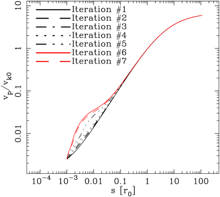
Figure 11.— Poloidal velocity for the fiducial wind as a function of distance along the flowlines, showing the evolution of the velocity over several iterations of the code. Line driving does significantly affect the magnetocentrifugal wind near the base, but magnetocentrifugal driving dominates at larger distances for this Eddington ratio. (In the first iteration in this plot, only magnetocentrifugal driving has been considered, so the “Iteration #1” curve shows the pure magnetocentrifugal wind case.)

It is important to note that considering non-Sobolev effects leads to large changes in $M_{\rm lines}$, the line force multiplier, found in the above calculations: “capping” the Sobolev absorption length-scale by the actual absorbing column length leads to smaller optical depths and larger line accelerations. This is illustrated in Figure 12, where the fiducial model has been calculated with the Sobolev approximation as well as our non-Sobolev treatment (see Section 3.3.2). The difference in force multiplier is due to the strict Sobolev treatment overestimating the column for the low-acceleration gas near the base of the wind. This relatively straightforward modification is very important to correctly estimate the optical depth, as can be seen in Figure 12.

Figure 12.— Comparison of the line force multiplier, $M_{\rm Lines}$ (see Eq. 4), for the case of our non-Sobolev method (defined in Section 3.3.2) and the strict Sobolev calculation. The over-estimate of the absorbing column in the Sobolev approximation leads to higher opacity in the gas (higher $t$) and thus lower acceleration.

Overall, in this section, the fiducial model has shown how the wind velocity, number density, column density, and radiative acceleration all interact to determine the final state of a magnetocentrifugal wind. These components have not previously been self-consistently combined in a magnetocentrifugal model, and so yield a new look at the state of these winds. In addition, the importance of the number densities and column densities to the final result are most apparent, and clearly merit further investigation, which will be addressed in §5.

5. Dependence of Wind Structure on Model Parameters

Having analyzed the fiducial model in detail, and observed how that model’s properties change with height, how sensitive are the trends in §4 to those fiducial parameters? This is an important question, and one of the key attributes of this self-similar model is that it allows some flexibility in the selection of initial parameters. In this section, we test for variations in the wind by examining how the wind changes as parameters are modified.

5.1. Variations with Shielding Column

One of the most difficult issues for radiative driving in AGNs is over-ionization of the wind. As shown in §4, as the wind accelerates and its density decreases, the magnetocentrifugal outflow can easily become too ionized to be efficiently accelerated to escape velocity solely by atomic lines. This is the problem of the “shielding gas” that was mentioned in §1: for pure radiative line-driving, some shielding gas is required to intercept the X-ray ionizing radiation so that the remaining UV resonant line photons can be absorbed by the wind and radiatively accelerate it to the escape velocity.

Some important papers have already been dedicated to examining the concept of shielding gas, such as Chelouche & Netzer (2003b, considering very detailed photoionization simulations of gas shields with constant column density) and Proga & Kallman (2004, where multidimensional hydrodynamics simulations with approximate radiative effects are considered). In contrast, the models presented here include a shield where the column density varies with height in a shielding wind, and where detailed photoionization simulations can be employed.

The MHD wind model presented here already launches a wind magnetocentrifugally, so it is immune to concerns of overionization. Is it therefore possible for a magnetocentrifugally-driven wind, with its commensurate drop in column density with height above the disk, to act as a shield, allowing for more efficient radiative acceleration beyond it? We can test this question by simply varying the shielding column in the fiducial model and checking the radiative acceleration seen by a wind launched behind the shield.

As shown in Figure 13, as the shielding column is increased from $N_{\rm H,shield,0}\sim 10^{21}$ to $10^{24}~{}{\rm cm}^{-2}$, line-driving in the wind increases from $\Gamma_{\rm lines}\sim 0.05$ to $\Gamma_{\rm lines}\sim 0.12$. (Recall that for this model, continuum driving is $\Gamma_{\rm continuum}\sim 0.01$.) This shows that, for large shielding columns ($N_{\rm H,shield,0}\sim 10^{24}~{}{\rm cm}^{-2}$), line driving can be up to an order of magnitude more effective than continuum-driving at the base of the wind. This increase in acceleration is due to the absorption of the ionizing radiation by the shield, which allows a lower ionization state in the wind, and more line-driving due to more atomic lines. It is also apparent that, as the shielding is increased, the resultant lower total flux at the base of the wind means that the onset of significant radiative acceleration is delayed: this accounts for the offset of maximum radiative acceleration from the disk surface as the shielding column is increased.

Further, in Figure 14, the ratio of radiative acceleration to magnetic acceleration along a streamline is shown. Since the MHD effects are still supplying most of the acceleration (with an acceleration roughly equal to and opposite that of gravity), the ratio of radiative to magnetic acceleration looks much like that in Figure 13. Magnetic effects dominate in these wind models, even when large columns of shielding are included.

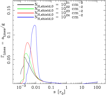
Figure 13.— Variations in line-driving as the magnetocentrifugally-launched shielding column is increased. With greater shielding columns, the wind is less highly ionized, leading to higher radiative acceleration near the base of the wind. Also, with increased shielding comes lower flux levels at the base of the wind, which displaces the onset of line-driving to larger distances from the launch point. (Continuum-driving is approximately constant at $a/g\sim 0.01$.)

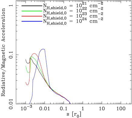
Figure 14.— As in Figure 13, but comparing the strength of the total radiative acceleration (both line and continuum acceleration) to the acceleration due to magnetic fields, where both are normalized relative to gravity. To compare with the magnetic field acceleration, the radiative acceleration is scaled by a geometrical factor (see Eq. 13) that yields the radiative acceleration along the streamline.

We have therefore shown that a magnetocentrifugal outflow can act as a shield and increase the efficiency of line-driving in the wind. However, it can also be seen that line-driving is important in these models only at the base of the wind. This arises not only from the drop in the shield’s column density with height above the disk, but the drop in the wind’s density as well (and the commensurate rise of the ionization parameter).

5.2. Variations with Initial Density

Owing to the increase of line-driving with decreasing ionization parameter, higher accelerations would also be expected at higher densities. Thus, we investigate the effect of changes in the initial density in the wind in Figures 15 and 16.

Displaying the effect of a range of initial densities, Figure 15 shows that line-driving is only effective in these magnetocentrifugal winds at relatively high densities. Since continuum driving is approximately constant (and relatively independent of density) at $a/g\sim 0.01$ for $L/L_{\rm Edd}=0.01$, any line-driving below that level is insignificant for these winds. Thus, for initial densities $n_{0}<10^{9}~{}{\rm cm}^{-3}$, line driving falls below the level of continuum driving and ceases to be important. For the highest density tested, $n_{0}=10^{11}~{}{\rm cm}^{-3}$, line driving dominates continuum driving for all locations in the wind. (The variations in each acceleration curve as a function of $s$ shown on this plot are chiefly due to variations in ionization parameter: line-driving is high near the disk due to shielding and the relatively high density, and rises towards the end of the streamline due to the dropping flux levels at large distances.)

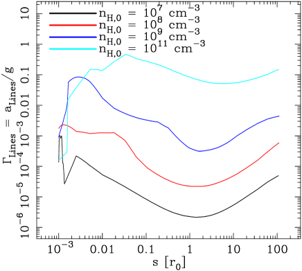
Figure 15.— Variations in line-driving with changes in the density at the base of the wind. Higher densities lead to smaller ionization parameters and much larger acceleration. (Continuum-driving is approximately constant at $a/g\sim 0.01$.)

Since $n_{0}$ clearly has a great impact on the radiative acceleration, how do such changes affect observables, such as the velocity? Figure 16 shows how the variation in radiative acceleration affects the poloidal velocity ($v_{\rm p}$) of the outflow. As the initial density and radiative acceleration increase, the wind’s velocity shows substantial variations from the pure magnetocentrifugal model (which dominates the $n_{0}=10^{7}~{}{\rm cm}^{-3}$ and $n_{0}=10^{8}~{}{\rm cm}^{-3}$ models). In the case of $n_{0}=10^{11}~{}{\rm cm}^{-3}$, where the greatest difference in $v_{\rm p}$ is seen, the velocity increases by a factor of $\sim 2$ to 3 close to the disk. Beyond the region close to the disk ($s/r_{0}>1$), however, magnetocentrifugal driving still dominates the final velocities for these winds. But the velocity differences near the disk may be observationally important, especially if acceleration near the base of the wind is the source of single-peaked emission lines (as in Murray & Chiang, 1997). If true, such emission lines may be critical in testing the differences between wind models.

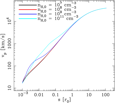
Figure 16.— As in Fig. 15, except that the change in velocity along the streamline is shown for the variety of densities. For this Eddington ratio, the magnetocentrifugal wind still dominates, but as the density increases, the importance radiative driving increases.

5.3. Variations with Radiative Column

Having already tested the more obvious parameters of the initial density and shield column density, we now turn to one of the most crucial parameters for the efficiency of line-driving: the optical depth in the lines.

Under normal circumstances, where the gas velocity is sufficiently low, or where the gas column is very low, the optical depths in the lines are simply governed by the ionic columns themselves. For large accelerations or large columns, however, the optical depths are dominated by the Sobolev length, which is defined as the distance over which the relative velocity between atoms is equal to the thermal width, so that a photon emitted by one atom could be absorbed by another within that Sobolev length (see §3.3.1). With the Eddington ratio in this magnetocentrifugal wind model ($L/L_{\rm Edd}=0.01$), both regimes can be important. Depending on the initial parameters prescribed, the wind column can be small enough such that the column alone determines the opacity in the wind (instead of the velocity) and therefore the amount of observed acceleration, so that the Sobolev length is not important. This is demonstrated in Figure 17, where the variation in line-driving with the radiatively accelerated wind column is presented (the shielding column is held constant). For the larger columns, the optical depth in the lines increases and the radiative acceleration decreases. For the smallest columns, very large radiative acceleration is predicted due to the low opacity in the lines. This is critical for these models, for at significantly high column, the wind would see no significant line driving (this is true for magnetocentrifugal wind columns with $N_{\rm H,rad,0}\gtrsim 10^{22}~{}{\rm cm}^{-2}$).

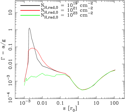
Figure 17.— Variations in line-driving as the radiative wind column is increased. As the wind thickness increases, the optical depth within of the lines within the magnetocentrifugal wind increases and line-driving drops in strength. (Continuum-driving is approximately constant at $a/g\sim 0.01$.)

5.4. Modifying the Eddington Ratio

Of key importance to applications to AGN is understanding the acceleration of outflows as a function of the Eddington ratio, $L/L_{\rm Edd}$. To investigate the impact of varying Eddington ratios in our model, we present Figure 18, which displays the radiative acceleration (both the combined line and continuum acceleration in panel a as well as the line driving in panel b) in the fiducial model for three different Eddington ratios: $L/L_{\rm Edd}=0.001,0.01,$ and $0.1$.

The largest variation in Figure 18a is the continuum driving increasing linearly with the Eddington ratio. As expected, the continuum acceleration, relative to gravity, is roughly equal to the Eddington ratio. The line driving, on the other hand, can be seen in both the deviations from the approximately constant continuum acceleration in Figure 18a and in Figure 18b.

We begin examining this figure by concentrating on the first three models in Figure 18, which have $N_{\rm H,shield,0}=10^{23}$ cm^-2. In these models in Figure 18a, the increase in acceleration due to line-driving, relative to the continuum-driving, decreases as the Eddington ratio increases. This can also be seen in Figure 18b, where the line-driving peaks near the disk ($s/r_{0}\lesssim 0.01$) for $L/L_{\rm Edd}=0.01$, but decreases for Eddington ratios an order of magnitude larger (where the gas is overionized) and an order of magnitude smaller (where the radiation field doesn’t have the momentum to accelerate the wind as strongly as at $L/L_{\rm Edd}=0.01$).

Now we turn to the fourth model in Figure 18, where we keep $L/L_{\rm Edd}=0.1$ but increase the shielding level to $N_{\rm H,shield,0}=10^{24}~{}$cm^-2. This model shows the importance of shielding gas for $L/L_{\rm Edd}=0.1$. The increase in $L/L_{\rm Edd}$ and the increase in shielding relative to the fiducial model allow for increased line radiative acceleration that jumps almost two orders of magnitude in strength near the base of the wind.

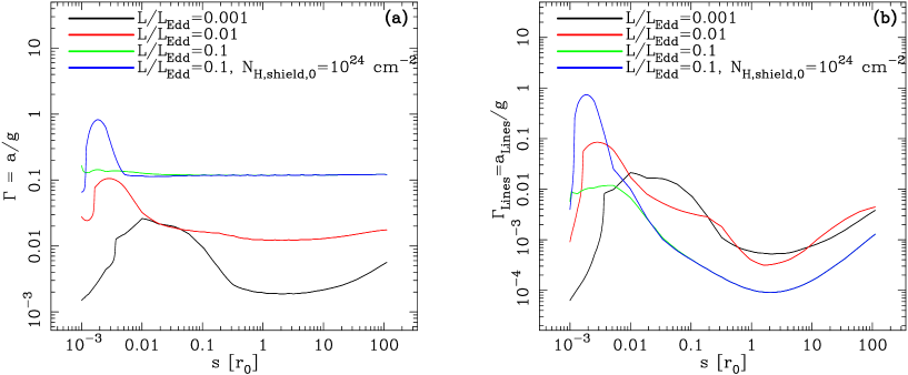
Figure 18.— Variation in both continuum and line driving (a) and line driving alone (b) when the Eddington ratio in the fiducial model is modified. The first three models all have $N_{\rm H,shield,0}=10^{23}$ cm^-2, while the last model has $N_{\rm H,shield,0}=10^{24}$ cm^-2. For lower Eddington ratios ($L/L_{\rm Edd}=0.001,0.01$) the gas is in a relatively low ionization state for line-driving to be important, and the acceleration departs from the pure continuum acceleration (which sets the acceleration relative to gravity to about the Eddington ratio). For a high Eddington ratio ($L/L_{\rm Edd}=0.1$), the gas is overionized and only continuum acceleration is important; raising the shielding to a nearly Compton-thick $N_{\rm H,shield,0}=10^{24}$ cm^-2 lowers the ionization state of the gas and allows much higher radiative acceleration.

6. Results

If magnetocentrifugal winds power outflows in AGNs, they must certainly be affected by the intense radiation field they experience; in turn, such winds will also influence the efficiency of radiative acceleration. This paper has explored the radiative transfer through these magnetocentrifugal winds, and how they both are affected by and affect radiative acceleration of outflows from AGNs. The model has been used to explore the detailed dynamics and ionization of a fiducial magnetocentrifugal disk wind, showing the inter-relation between shielding column, initial number density, outflow velocity, Eddington ratio, and acceleration.

As a result of this study, these models have shown:

1. A magnetocentrifugal outflow, acting as a “shield”, can improve the efficiency of line-driving by factors of approximately two to three $N_{\rm H,shield,0}=10^{23}~{}$cm^-2 (§5.1) and by up to almost two orders of magnitude for $N_{\rm H,shield,0}=10^{24}~{}$cm^-2 (§5.4). A magnetocentrifugal wind has the advantage that it can be accelerated without regard to the ionization state, whereas radiatively-driven winds must have a low ionization parameter in order for a critical abundance of atomic lines to be present. Therefore, magnetocentrifugal winds could play an important role in acting as a radiation shield and allow large radiative accelerations. It may also be possible that pressure differences (MCGV95) or disk photons (Proga & Kallman, 2004) may help “lift” the shield; neither of those effects are considered here. Later work with this model will include the effect of disk-emitted photons.

2. The efficiency of line-driving is strongly dependent on the density at the base of the wind (§5.2). This is due to the very critical dependence of line acceleration on the ionization parameter. The lower the ionization state, the more lines exist to aid in the momentum transfer from outward-streaming photons. The density at the base of the disk is therefore crucial to setting to line-driving within these magnetocentrifugal models.

3. Small columns ($N_{\rm H,rad,0}\lesssim 10^{21}~{}{\rm cm}^{-2}$) within magnetocentrifugal winds can be significantly accelerated by line-driving (§5.3). This point demonstrates the importance of “non-Sobolev” effects; i.e., that at low columns, the optical depths in the lines drop below the opacity given by the Sobolev length, and at such low columns, the radiative acceleration can be underestimated by the simple Sobolev approximation.

In addition, by examining the fiducial model and the above cases where model parameters are varied, these solutions have displayed the importance of considering the detailed interaction between the dynamics and photoionization in AGN outflows. Calculations of the ionization parameter along the flow and in the variation of shielding and optical depth along the flow are central issues to modeling these winds. The issues outlined above are a few of the dependences that arise from such modeling, and may indeed (by the variation in acceleration and therefore velocity along the streamlines) lead to tests to observationally determine the physics of wind launching in AGNs.

Thus, while this model has been developed to help address the above questions about shielding and the affects of radiative driving on magnetocentrifugal winds, the solutions available are not limited to the above, examined cases. Future papers will study further the variation of radiative acceleration on model parameters such as the SED, atomic line lists used to calculate the acceleration, initial densities, Eddington ratios, and other parameters of the model. The model can also be used to explore the absorption and emission features from such a wind, as well as, for instance, the possible role of “clouds” within a continuous wind (Everett et al., 2002). In addition, this model is in no way constrained to only study AGNs. The same basic physical framework could also be employed to study winds from accretion disks surrounding young stellar objects or cataclysmic variables.

7. Acknowledgments

I gratefully acknowledge my advisor, Arieh Königl, for many useful conversations throughout the course of this project. In addition, many thanks to Gary Ferland and his collaborators for developing Cloudy, making it freely available, and supporting it. The referee’s comments were very helpful, and those comments helped improve the paper. Thanks also to David Ballantyne, Pat Hall, Lewis Hobbs, John Kartje, Ruben Krasnopolsky, Bob Rosner, Nektarios Vlahakis, and Don York for valuable comments. This work would not have been possible without the generous support of NASA’s ATP program, in this case via grant NAG5-9063, and the support of the Natural Sciences and Engineering Research Council of Canada. This research has made use of NASA’s Astrophysics Data System.

Appendix A Appendix A: Derivation of the Self-Similar Centrifugal Wind Equations

In this appendix, a rederivation of the system of self-similar wind equations for the magnetocentrifugal wind is presented. The equations utilized in this calculation advance upon those presented in BP82 and KK94: the wind not only has an arbitrary density power-law index, $b$, as in KK94, but energy conservation is not required. Since the radiation field continually inputs energy into the outflow, this is an important modification that was not fully considered in the derivation presented in KK94.

First, a stationary, axisymmetric, ideal, cold MHD flow in cylindrical coordinates $(r,\phi,z)$ is assumed. The equations are based on both the radial and vertical momentum equations:

$$v_{r}\frac{\partial v_{r}}{\partial r}+v_{z}\frac{\partial v_{r}}{\partial z}-\frac{v_{\phi}^{2}}{r} = -\rho\frac{\partial\Phi}{\partial r}-\frac{B_{z}}{4\pi}\left(\frac{\partial B_{z}}{\partial r}-\frac{\partial B_{r}}{\partial z}\right)-\frac{B_{\phi}}{4\pi r}\frac{\partial(rB_{\phi})}{\partial r}$$ (A1)

$$\rho(\mathbf{v}\cdot\mathbf{\nabla})v_{z} = -\rho\frac{\partial\Phi}{\partial z}-\frac{1}{8\pi}\frac{\partial B^{2}}{\partial z}+\frac{1}{4\pi}(\mathbf{B}\cdot\mathbf{\nabla})B_{z},$$ (A2)

where $\mathbf{v}$ is the fluid velocity and $\mathbf{B}$ is the magnetic field. The thermal term is neglected in the limit that thermal affects are much less important than magnetocentrifugal and radiative-driving effects. $\Phi$ is the effective gravitational potential, defined as

$$\Phi=-[1-\Gamma(\theta)]\frac{GM_{\bullet}}{(r^{2}+z^{2})^{1/2}},$$ (A3)

where $M_{\bullet}$ is the mass of the central black hole, and $\Gamma(\theta)$ gives the local radiative-to-gravitational radial acceleration (see eq. [1]).

These equations are solved by first stipulating mass conservation,

$$\mathbf{\nabla}\cdot(\rho\mathbf{v})=0,$$ (A4)

and then relating the flow velocity to the magnetic field via

$$\mathbf{v}(\mathbf{r})=\frac{k\mathbf{B}(\mathbf{r})}{4\pi\rho(\mathbf{r})}+\mathbf{\omega}(\mathbf{r})\times\mathbf{r},$$ (A5)

(e.g., Chandrasekhar, 1956; Mestel, 1961), where $k/4\pi$ is the ratio of mass flux to magnetic flux, and $\mathbf{\omega}(\mathbf{r})$ and $\rho(\mathbf{r})$ are the field angular velocity and gas mass density of the flow, respectively. Both $\omega$ and $k$ are constant along magnetic fieldlines. In addition, while the specific energy is not constant, the total specific angular momentum

$$l=rv_{\phi}-\frac{rB_{\phi}}{k}$$ (A6)

is conserved.

Self-similarity is then imposed on this system by specifying

$$\mathbf{r} = [r_{0}\xi(\chi),\phi,r_{0}\chi],$$ (A7)

$$\mathbf{v} = [\xi^{\prime}(\chi)f(\chi),g(\chi),f(\chi)]v_{k,0},$$ (A8)

where $v_{\rm k,0}$ is the Keplerian speed at the base of the outflow, $v_{\rm k,0}=(GM_{\bullet}/r_{0})^{1/2}$, and the prime indicates differentiation with respect to $\chi$. At the same time, the above constants are re-expressed in dimensionless form:

$$\lambda \equiv \frac{l}{(GM_{\bullet}r_{0})^{1/2}},$$ (A9)

$$\kappa \equiv \frac{k(1+{\xi^{\prime}}_{0}^{2})^{1/2}}{B_{p,0}}v_{k,0},$$ (A10)

where $B_{p,0}$ is the poloidal magnetic field strength at the base of the wind.

As in KK94, a general power-law scaling of the density and magnetic field along the disk’s surface is defined:

$$\rho_{0} \propto r_{0}^{-b},$$ (A11)

$$B_{0} \propto r_{0}^{-(b+1)/2}.$$ (A12)

With this self-similar specification, the radial and vertical momentum equations become, after some simplification:

$$\frac{f\xi^{\prime}m^{\prime}}{\kappa\xi J}-\frac{f^{2}\xi^{\prime}}{\xi J}+\xi^{\prime\prime}f^{2}-\frac{(\lambda m-\xi^{2})^{2}}{\xi^{3}(m-1)^{2}} = -\xi[1-\Gamma(\theta)]S^{3}-\frac{f}{\kappa\xi J^{2}}\left(\frac{-(1+\xi^{\prime 2})(b+1)}{2}+\right.$$ (A13)

$$\left.\frac{(\chi+\xi\xi^{\prime})\xi^{\prime}}{\xi}-\frac{\xi^{\prime\prime}}{JS^{2}}\right)-\frac{\kappa f}{\xi}\frac{(\lambda-\xi^{2})}{(m-1)}$$

$$\left[\frac{(\lambda-\xi^{2})}{(m-1)}\frac{(-b+1)}{2}+\right.$$

$$\left.\chi\left(\frac{2\xi\xi^{\prime}}{(m-1)}+\frac{(\lambda-\xi^{2})m^{\prime}}{(m-1)^{2}}\right)\right],$$

$$\frac{f}{\kappa\xi J}(m^{\prime}-f\kappa\xi^{\prime}J+f\kappa\xi\chi\xi^{\prime\prime}) = -[1-\Gamma(\theta)]\chi S^{3}+\frac{f\xi^{\prime}}{\kappa\xi J^{2}}\left(\frac{-(1+\xi^{\prime 2})(b+1)}{2}+\right.$$ (A14)

$$\left.\frac{(\chi+\xi\xi^{\prime})\xi^{\prime}}{\xi}-\frac{\xi^{\prime\prime}(\chi^{2}+\xi^{2})}{J}\right)-$$

$$\xi^{\prime}\kappa f(\lambda-\xi^{2})\left(\frac{(b+1)(\lambda-\xi^{2})-2(\lambda+\xi^{2})}{2\xi(m-1)^{2}}\right)+$$

$$\frac{(\lambda-\xi^{2})^{2}m^{\prime}\kappa f}{(m-1)^{3}},$$

where

$$m \equiv \frac{4\pi\rho v_{p}^{2}}{B_{p}^{2}}=\kappa\xi fJ={\rm square~{}of~{}poloidal~{}Alfv\acute{e}n~{}Mach~{}number},$$ (A15)

$$\kappa \equiv \frac{k(1-{\xi^{\prime}}_{0}^{2})^{\frac{1}{2}}v_{k,0}}{B_{p,0}}={\rm dimensionless~{}ratio~{}of~{}mass~{}flux~{}to~{}magnetic~{}flux},$$ (A16)

$$\lambda \equiv \frac{l}{(GMr_{0})^{\frac{1}{2}}}={\rm normalized~{}angular~{}momentum},$$ (A17)

$$J \equiv \xi-\chi\xi^{\prime},$$ (A18)

$$S \equiv 1/\sqrt{\xi^{2}+\chi^{2}}.$$ (A19)

The two equations (A13) and (A14) define the differential equations for $m^{\prime}$ and $\xi^{\prime\prime}$, which are, respectively, the spatial gradient in the poloidal Alfvén mach number (gradient with respect to height, $\chi$) and the (cylindrical) radial velocity gradient (again with respect to $\chi$).

One can see from close inspection of the above equations that many of the terms have a denominator of $(m-1)$, showing that when the gas crosses the Alfvén point (where $m=1$), the equations become singular. Rewriting and solving the $m^{\prime}$ equation for the value of $m^{\prime}$ at the Alfvén singular point:

$$m^{\prime}_{A} = 2\xi J[-8\chi\kappa^{2}\lambda m^{\prime}\xi^{\prime}J^{3}+4(1+b)\kappa^{2}\lambda\xi^{\prime 2}J^{2}(\chi+\xi\xi^{\prime})+m^{\prime 2}(\chi+\xi\xi^{\prime})(-2\kappa^{2}\lambda^{2}S+$$ (A21)

$$(1+b)+2\kappa^{2}\lambda^{3}-4\chi\kappa^{2}\lambda^{\frac{3}{2}}(\lambda-S)\xi^{\prime}+((1+b)+2\chi^{2}\kappa^{2}\lambda(\lambda-S))\xi^{\prime 2}+2\kappa^{2}\lambda\Gamma(\theta)J^{2})]/$$

$$\left[4\xi J\left(\frac{4\kappa^{2}\lambda\xi^{\prime 2}J^{2}}{S^{2}}+m^{\prime 2}(\chi+\xi\xi^{\prime})^{2}\right)\right].$$

This constraint is used to start the integral at the Alfvén point with the value of $m^{\prime}_{A}$ given by equation (A21).

As covered in the main text, these equations are solved using a “shooting algorithm,” integrating from both the Alfvén point and the disk surface towards an intermediate point. Matching the integrals of three first-order equations (given by the first-order equation for $m^{\prime}$ and the second-order equation for $\xi^{\prime\prime}$ in eqs. A13 and A14) at the common point allows us to solve for the three free parameters in the system: $\xi^{\prime}_{0}$, $\xi^{\prime}_{A}$, and $\chi_{A}$.

References

- Abbott (1980) Abbott, D.C. 1980, ApJ, 242, 1183
- Antonucci (1993) Antonucci, R. 1993, ARA&A, 31, 473
- Arav et al. (1994) Arav, N., Li, Z., & Begelman, M.C. 1994, ApJ, 432, 62
- Arav et al. (1995) Arav, N., Korista, K.T., Barlow, T.A., Begelman, M.C. 1995, Nature, 376, 576
- Arav (1996) Arav. N. 1996, ApJ, 465, 617
- Arav et al. (1998) Arav, N., Barlow, T.A., Laor, A., Sargent, W.L.W, & Blandford, R.D. 1998, MNRAS, 297, 990
- Arnaud & Raymond (1992) Arnaud, M. & Raymond, J. 1992, ApJ, 398, 394
- Baldwin et al. (1991) Baldwin, J., Ferland, G.J., Martin, P.G., Corbin, M., Cota, S., Peterson, B.M., & Slettebak, A. 1991, ApJ, 374, 580
- Baldwin et al. (1995) Baldwin, J., Ferland, G.J., Korista, K., Verner, D. 1995, ApJ, 455, 119
- Balsara & Krolik (1993) Balsara, D. & Krolik, J.H. 1993, ApJ, 402, 109
- Blandford & Königl (1979) Blandford, R.D., & Königl, A. 1979, Astrophys. Lett., 20, 15
- Blandford & Payne (1982) Blandford, R.D., & Payne, D.G. 1982, MNRAS, 199, 883 (BP82)
- Blandford (2001) Blandford, R.D. 2001, in ASP Conf. Ser. 224, Probing the Physics of Active Galactic Nuclei by Multiwavelength Monitoring, ed. B. M. Peterson, R. S. Polidan & R. W. Pogge (San Francisco: ASP), 499
- Bottorff et al. (1997) Bottorff, M., Korista, K.T., Shlosman, I., & Blandford, R.D. 1997, ApJ, 479, 200
- Bottorff, Korista, & Shlosman (2000) Bottorff, M., Korista, K.T., & Shlosman, I. 2000, ApJ, 537, 134
- Bottorff & Ferland (2001) Bottorff, M., & Ferland, G. 2001, ApJ, 549, 118
- Cassinelli (1979) Cassinelli, J. P. 1979, ARA&A, 17, 275
- Castor et al. (1975) Castor, J.I., Abbott, D.C., & Klein, R.I. 1976, ApJ, 195, 157
- Chandrasekhar (1956) Chandrasekhar, S. 1956, ApJ, 124, 232
- Chelouche & Netzer (2001) Chelouche, D., Netzer, H. 2001, MNRAS, 326, 916
- Chelouche & Netzer (2003a) Chelouche, D., Netzer, H. 2003, MNRAS, 344, 223
- Chelouche & Netzer (2003b) Chelouche, D., Netzer, H. 2003, MNRAS, 344, 233
- Chiang & Blaes (2003) Chiang, J. & Blaes, O. 2003, ApJ, 586, 97
- Contopoulos & Lovelace (1994) Contopoulos, J., & Lovelace, R.V.E. 1994, ApJ, 429, 139
- Crenshaw et al. (1999) Crenshaw, D.M., Kraemer, S.B., Boggess, A., Maran, S.P., Mushotzky, R.F., Wu, C. 1999, ApJ, 516, 750
- Crenshaw, Kraemer, & George (2003) Crenshaw, D.M., Kraemer, S.B., George, I.M. 2003, ARAA, 41, 117
- de Kool & Begelman (1995) de Kool, M., & Begelman, M.C. 1995, ApJ, 455, 448
- Deluit (2004) Deluit, S.J. 2004, A&A, 415, 39
- Draine & Lee (1984) Draine B.T., & Lee, H.M. 1984, ApJ, 285, 89
- Drew & Boksenberg (1984) Drew, J.E., & Boksenberg, A. 1984, MNRAS, 211, 813
- Elvis (2000) Elvis, M. 2000, ApJ, 545, 63
- Elvis, Risaliti, & Zamorani (2002) Elvis, M., Risaliti, G., & Zamorani, G. 2002, ApJ, 565, L75
- Emmering et al. (1992) Emmering, R.T., Blandford, R.D., & Shlosman, I. 1992, ApJ, 385, 460
- Everett et al. (2002) Everett, J.E., Königl, A., Arav, N. 2002, ApJ, 569, 671
- Fath (1909) Fath, E.A. 1909, Lick Obs. Bull., 149, 71
- Feldmeier & Shlosman (1999) Feldmeier, A. & Shlosman, I. 1999, ApJ, 526, 344
- Ferland et al. (1998) Ferland, G.J., Korista, K.T., Verner, D.A., Ferguson, J.W., Kingdon, J.B., & Verner, E.M. 1998, PASP, 110, 761
- Ferreira (2003) Ferreira, J. 2003 in Star Formation and the Physics of Young Stars, eds. J. Bouvier and J.-P. Zahn (Les Ulis: EDP Sciences), 229 (astro-ph/0311621)
- Friend & MacGregor (1984) Friend, D.B. & MacGregor, K.B. 1984, ApJ, 282, 591
- Fromerth & Melia (2001) Fromerth, M.J & Melia, F. 2001, ApJ, 549, 205
- Ganguly et al. (2001) Ganguly, R., Bond, N.A., Charlton, J.C., Eracleous, M., Brandt, W.N., & Churchill, C.W. 2001, ApJ, 549, 133
- Gregori et al. (2000) Gregori, G., Miniati, F., Ryu, D., & Jones, T.W. 2000, ApJ, 543, 775
- Hamann et al. (2001) Hamann, F.W., Barlow, T.A., Chaffee, F.C., Foltz, C.B., & Weymann, R.J. 2001, ApJ, 550, 142
- Hartley et al. (2002) Hartley, L.E., Drew, J.E., Long, K.S., Knigge, C., Proga, D. 2002, MNRAS, 332, 127
- Kartje (1995) Kartje, J.F. 1995, ApJ, 452, 565
- Kartje et al. (1999) Kartje, J.F., Königl, A., & Elitzur, M. 1999, ApJ, 513, 180
- Krolik (1999) Krolik, J.H. 1999, Active Galactic Nuclei: From the Central Black Hole to the Galactic Environment (Princeton: Princeton University Press)
- Krolik & Kriss (2001) Krolik, J.H. & Kriss, G.A. 2001, ApJ, 561, 684
- Königl & Kartje (1994) Königl, A., & Kartje, J.F. 1994, ApJ, 434, 446 (KK94)
- Königl & Pudritz (2000) Königl, A., & Pudritz, R.E. 2000 in Protostars & Planets IV, ed. V. Mannings, A. P. Boss, S. S. Russell (Tucson: University of Arizona Press), 759
- Kraemer et al. (2002) Kraemer, S.B., Crenshaw, D.M., George, I.M., Netzer, H., Turner, T.J., Gabel, J.R. 2002, ApJ, 577, 98
- Krasnopolsky, Li, & Blandford (1999) Krasnopolsky, R., Li, Z.-Y.,Blandford, R. 1999, ApJ, 526, 631
- Kuncic, Celotti, & Rees (1997) Kuncic, Z., Celotti, A., Rees, M.J. 1997, MNRAS, 284, 717
- Laor & Brandt (2002) Laor, A., & Brandt, W.N. 2002, ApJ, 569, 641
- Martin & Rouleau (1991) Martin, P.G., & Rouleau, F. 1991, in Extreme Ultraviolet Astronomy, eds, Malina, R.F., Bowyer S., Pergamon Press, Oxford, 341
- Mathews & Ferland (1987) Mathews, W.G., & Ferland, G.J. 1987, ApJ, 323, 456 (MF87)
- Mathis, Rumpl, & Nordsieck (1977) Mathis, J.S., Rumpl, W., & Nordsieck, K.H. 1977, ApJ, 217, 425
- Meier et al. (1997) Meier, D.L., Edgington, S., Godon, P., Payne, D.G., Lind, K.R. 1997, Nature, 388, 350
- Mestel (1961) Mestel, L. 1961, MNRAS, 122, 473
- Mihalas & Weibel-Mihalas (1999) Mihalas, D. & Weibel-Mihalas, B. 1999, Foundations of Radiation Hydrodynamics, (Mineola:Dover Publications, Inc.)
- Murray & Chiang (1997) Murray, N., & Chiang, J. 1997, ApJ, 474, 91
- Murray et al. (1995) Murray, N., Chiang, J., Grossman, S.A., & Voit, G.M. 1995, ApJ,451, 498 (MCGV95)
- Netzer (1990) Netzer, H. 1990, in Active Galactic Nuclei, Saas-Fee Advanced Course 20 (Berlin: Springer-Verlag), 57
- Ouyed & Pudritz (1997) Ouyed, R., Pudritz, R.E. 1997, ApJ, 482, 712
- Ouyed et al. (1997) Ouyed, R., Pudritz, R.E., Stone, J.M. 1997, Nature, 385, 409
- Pereyra et al. (2004) Pereyra, N.A., Owocki, S.P., Hillier, D.J., Turnshek, D.A. 2004, ApJ, 608, 454
- Peterson (1997) Peterson, B.M. 1997, An Introduction to Active Galactic Nuclei, (New York:Cambridge University Press)
- Powell (1970) Powell, M.J.D. 1970, in Numerical Methods for Nonlinear Algebraic Equations, ed, P. Rabinowitz (New York: Gordon and Breach).
- Proga (1999) Proga, D. 1999, MNRAS, 304, 938
- Proga (2000) Proga, D. 2000, ApJ, 538, 684
- Proga (2003) Proga, D. 2003, ApJ, 585, 406
- Proga, Stone & Drew (1998) Proga, D., Stone, J.M., Drew, J.E. 1998, MNRAS, 295, 595
- Proga, Stone, & Kallman (2000) Proga, D., Stone, J.M., & Kallman, T.R. 2000, ApJ, 543, 686, PSK00
- Proga & Kallman (2004) Proga, D., & Kallman, T.R, 2004, accepted to ApJ (astro-ph/0408293)
- Rees (1987) Rees, M.J. 1987, MNRAS, 228, 47P
- Reichard et al. (2003) Reichard, T.A., Richards, G,T., Hall, P.B., Schneider, D.P., Vanden Berk, D,E., Fan, X., York, D.G.; Knapp, G.R.; Brinkmann, J. 2003, AJ, 126, 2594
- Risaliti & Elvis (2004) Risaliti, G & Elvis, M. 2004, in Supermassive Black Holes in the Distant Universe, ed. A. J. Barger (Boston: Kluwer)
- Romanova et al. (1997) Romanova, M.M., Ustyugova, G.V., Koldoba, A.V., Chechetkin, V.M., Lovelace, R.V.E. 1997, ApJ, 482, 708
- Safier (1993) Safier, P. 1993, ApJ, 408, 115
- Sobolev (1958) Sobolev, V.V. 1958 in Theoretical Astrophysics, ed. V.A. Ambartsumian (London: Pergamon)
- Spruit (1996) Spruit, H.C. 1996 in Physical processes in Binary Stars, eds. R.A.M.J. Wijers, M.B. Davies & C.A. Tout, (Dordrecht: Kluwer) (astro-ph/9602022)
- Steenbrugge et al. (2003) Steenbruge, K.C., Kaastra, J.S., de Vries, C.P., Edelson, R. 2003, A&A in press (astro-ph/0302493)
- Stevens & Kallman (1990) Stevens, I.R, & Kallman, T.R. 1990, ApJ, 365, 321
- Tielens et al. (1994) Tielens, A.G.G.M., McKee, C.F., Seab, C.G., Hollenbach, D.J. 1994, ApJ, 431, 321
- Tran (2003) Tran, H.D. 2003, ApJ, 583, 632
- Urry & Padovani (1995) Urry, C.M., & Padovani, P. 1995, PASP, 107, 803
- Ustyugova et al. (1995) Ustyugova, G.V., Koldoba, A.V., Romanova, M.M., Chechetkin, V.M., & Lovelace, R.V.E. 1995, ApJ, 439, L39
- Verner & Ferland (1996) Verner, D.A., & Ferland, G.J. 1996, ApJS, 103, 467
- Verner et al. (1996) Verner, D.A., Verner, E.M., & Ferland, G.J. 1996, Atomic Data Nucl. Data Tables, 64, 1
- Vitello & Shlosman (1988) Vitello, P.A.J, & Shlosman, I. 1988, ApJ, 327, 680
- Vlahakis et al. (2000) Vlahakis, N., Tsinganos, K., Sauty, C., Trussoni, E., 2000, MNRAS, 318, 417
- Wardle & Königl (1993) Wardle, M., & Königl, A. 1993, ApJ, 410, 218
- Weber & Davis (1967) Weber, E.J. & Davis, L. Jr. 1967, ApJ, 148, 217
- Weymann et al. (1991) Weymann, R.J., Morris, S.L., Foltz, C.B., Hewett, P.C. 1991, ApJ, 373, 23