Galaxy clustering from COMBO-17: The halo occupation distribution at $\langle z\rangle=0.6$

We present measurements of galaxy clustering at redshift $\langle z\rangle=0.6$ using $10\,360$ galaxies with photometric redshifts over an area of 0.78 deg² from the COMBO-17 survey. To obtain a result that is unaffected by redshift uncertainties, we calculate the projected correlation function $w(r_{p})$, giving results for red sequence and blue cloud galaxies separately. The correlation function of the red galaxies displays clear deviations from a power law at comoving separations around 1 to $3{\,h^{-1}\,\rm Mpc}$, and similar but weaker trends are suggested by the data for the blue galaxies. To interpret these results, we fit the correlation functions with analytical predictions derived from a simple halo occupation model. This combines linear clustering of the underlying mass with a description of the number of galaxies occupying each dark-matter halo (the halo occupation distribution). If the occupation numbers are taken to be a simple power law $N\propto\smash{M^{\alpha}}$, then $\alpha\simeq 0.5$ and $\alpha\simeq 0.2$ for red and blue galaxies respectively. These figures are little different from the values required to fit present-day clustering data. The power-spectrum shape is assumed to be known in this exercise, but we allow the data to determine the preferred value of $\sigma_{8}$, the linear power-spectrum normalization. The average normalization inferred from red and blue galaxies at $\langle z\rangle=0.6$ is $\sigma_{8}=1.02\pm 0.17$ at zero redshift, consistent with independent estimates of this local value. This agreement can be regarded as a verification of the hierarchical growth of the halo mass function.

1 Introduction

In current models of galaxy formation, structure grows hierarchically from small Gaussian density fluctuations. Galaxies are presumed to form within virialized dark matter haloes when the baryonic gas cools and condenses into stars (e.g. Cole et al. 2000). The formation and evolution of galaxies should thus be closely tied to the merging history of dark matter haloes. This paper uses measurements of galaxy clustering at intermediate redshift to test this basic picture.

The complex relation between galaxies and dark matter has become clearer only slowly. Empirically, galaxies display biased clustering in which the amplitude of their correlations varies with galaxy type: older galaxies are generally much more strongly clustered than young, starforming galaxies, and bright galaxies are more strongly clustered than faint galaxies (e.g. Davis & Geller 1976; Norberg et al. 2002; Phleps & Meisenheimer 2003). It is generally believed that such trends can be understood through the tendency for dark-matter haloes to display clustering that is larger for rare massive haloes (e.g. Cole & Kaiser 1989; Mo & White 1996; Sheth & Tormen 1999).

However, a long-standing challenge has been to understand how these ideas could be implemented in the context of Cold Dark Matter (CDM) models. The galaxy correlation function has long been known to be extremely close to a single power law (Totsuji & Kihara 1969, Peebles 1974), and yet this is not the case for the nonlinear mass correlations in a CDM model. Here, the matter correlation function rises above a best-fit power law on scales $r\la 1{\,h^{-1}\,\rm Mpc}$ and falls below it again on scales $r\la 0.2{\,h^{-1}\,\rm Mpc}$ (Jenkins et al. 1998 and references therein). This puzzle was only resolved when it became clear that the correlation function of dark matter haloes (including subhaloes inside large host haloes) differs significantly from the correlation function of the mass. In practice, the predicted correlation function of galaxy-scale haloes follows a power law down to $100\,h^{-1}$ kpc, with an amplitude and slope similar to the data on real galaxies (Kravtsov & Klypin 1999; Neyrinck et al. 2004; Kravtsov et al. 2004; Tasitsiomi et al. 2004). This phenomenon underlies the considerable scale-dependent bias predicted by semianalytic and hydrodynamic simulation models of galaxy formation (Colín et al. 1999; Kauffmann et al. 1999; Pearce et al. 1999; Benson et al. 2000; Cen & Ostriker 2000; Somerville et al. 2001; Yoshikawa et al. 2001; Weinberg et al. 2004).

These developments in turn stimulated a simpler and more direct insight into bias and its dependence on scale, through the so-called halo model (e.g. Jing 1998; Seljak 2000; Peacock & Smith 2000; Cooray & Sheth 2002 and references therein). Here, the shape of the correlation function is determined by the linear clustering of the dark matter, and the relation of the galaxies to the dark matter halos in which they reside (the Halo Occupation Distribution; HOD). In particular, a break in slope is expected when the correlation function changes from being dominated by pair counts of galaxies in separate dark matter halos to the small-scale regime, where pairs come from two galaxies that reside in the same halo. Any pure power law correlation function would require coincidental alignment of these two terms, and indeed analyses of the two-point correlation function of galaxies in the local universe have detected small deviations from the power-law form (Hawkins et al. 2003a; Zehavi et al. 2004, 2005; Abazajian et al. 2005).

In this paper, we use the COMBO-17 survey (Wolf et al. 2004) to carry out a similar investigation of the exact shape of the correlation function at higher redshifts. We calculate the projected correlation function $w(r_{p})$ for red sequence and blue cloud COMBO-17 galaxies (following the definition of Bell et al. 2004), in the redshift bin $0.4<z<0.8$. By comparing these results to the predictions of the halo model, we are able to infer the mean number of galaxies per halo of a given mass (the halo occupation number) and also the $z=0$ power-spectrum normalization $\sigma_{8}$ (the rms density variation averaged over $8h^{-1}$ Mpc spheres).

This paper is structured as follows: The COMBO-17 survey and the data used in this analysis are briefly described in Sect. 2. The halo model is introduced in Sect. 3. The method used to estimate the projected correlation function is explained in Sect. 4. In Sect. 5 we investigate the shape of the correlation function for red sequence and blue cloud galaxies, and in Sect. 6 the results are discussed. We assume a cosmological geometry taken from the WMAP results (Spergel et al. 2003, 2006) and the final 2dFGRS power spectrum results (Cole et al. 2005): a flat model with $\Omega_{m}=0.25$. All lengths quoted are in comoving units. Normally, we show explicit dependence on $h$ (which denotes $H_{0}/100\rm\,km\,s^{-1}\,Mpc^{-1}$); but for absolute magnitudes we suppress this dependence, so that $M_{B}$ denotes $M_{B}-5\log_{10}h$.

2 Data base: The COMBO-17 Survey

To date, COMBO-17 (Classifying Objects with Medium Band Observations in 17 filters) has surveyed three disjoint $\sim 31^{\prime}\times 30^{\prime}$ southern equatorial fields (for their coordinates see Wolf et al. 2003) to deep limits in $5$ broad and $12$ medium passbands, covering wavelengths from $400$ to $930$ nm. A detailed description of the survey along with filter curves can be found in Wolf et al. (2004). All observations were carried out using the Wide Field Imager at the MPG/ESO 2.2 m-telescope on La Silla, Chile.

In each filter, typically $10$ to $20$ individual exposures were taken (up to $50$ for ultradeep $R$-band images totalling $20$ ks with seeing $\la 0\aas@@fstack{\prime\prime}8$). Galaxies were detected on the deep $R$-band images by using SExtractor (Bertin & Arnouts 1996). The spectral energy distributions (SEDs) for $R$-band detected objects were measured by performing seeing-adaptive, weighted-aperture photometry in all $17$ frames at the position of the $R$-band detected object. All magnitudes are quoted with a Vega zero point.

Using the 17-band photometry, objects are classified using a scheme based on template spectral energy distributions (Wolf et al. 2001b, a). The classification algorithm basically compares the observed colours of each object with a colour library of known objects. This colour library is assembled from observed and model spectra by synthetic photometry performed using an accurate representation of the instrumental characteristics of COMBO-17. For galaxy classification, we use PÉGASE model spectra (see Fioc & Rocca-Volmerange 1997 for an earlier version of the model). The template spectra are a two-dimensional age/reddening sequence, in which a fixed exponential star formation timescale $\tau=1$ Gyr is assumed, ages vary between $50$ Myr and $15$ Gyr, and the reddening $E(B-V)$ can be as large as $0.5$ mag, adopting a Small Magellanic Cloud Bar extinction curve. Note that we do not apply any morphological star/galaxy separation or use other criteria.

Using a minimum variance estimator, each object is assigned a redshift (if it is not classified as a star). The redshift errors in this process depend on magnitude and type of the object, and for galaxies can be approximated by

$$\frac{\sigma_{z}}{(1+z)}=0.007\left(1+10^{0.8(R-21.6)}\right)^{1/2}\leavevmode\nobreak\ .$$ (1)

The galaxy redshift estimate quality has been tested by comparison with spectroscopic redshifts for almost 1000 objects (see Wolf et al. 2004). At bright limits $R<20$, the redshifts are accurate to $\sigma_{z}/(1+z)\simeq 0.01$, and the error is dominated by mismatches between template and real galaxy spectra. This error can contain a systematic component that is dictated by the exact filter placement, but these ‘redshift focusing’ effects are of the order of magnitude of the random redshift errors for $z<1$ and are unimportant for the current analysis. At the median apparent magnitude $R\simeq 23$, $\sigma_{z}/(1+z)\sim 0.02$. For the faintest galaxies, the redshift accuracy approaches those achievable using traditional broadband photometric surveys, $\sigma_{z}/(1+z)\ga 0.05$. We thus restricted our analysis to galaxies with $I<23$.

Fig. 1 shows the redshift distribution of the $22\,310$ COMBO-17 galaxies between $z=0.2$ and $z=1.2$ (with $I<23$ and $M_{B}<-18$). The peak at $z=0.733$ in Fig. 1 is due to a real structure in the Chandra Deep Field South, which has been spectroscopically confirmed (Gilli et al. 2003). In order to define a volume limited sample, we restrict our analysis to the redshift range $0.4<z<0.8$ and galaxies brighter than $M_{B}=-18$, which leaves us with $10\,360$ galaxies for the analysis. Note that $B$-band luminosities can be determined directly without any $K$-correction uncertainty, based on the photometry in our 17 filters between $400$ and $930$ nm and an interpolation of the corresponding template spectra. We do not apply any evolutionary corrections.

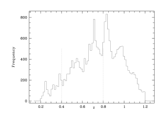
Figure 1: The redshift distribution for galaxies with $I<23$ and $M_{B}<-18$ in the three COMBO-17 fields. The dotted lines indicate the redshift range over which we define a volume-limited sample for the clustering analysis.

The distribution of the redshift errors for all galaxies in our subsample with $I<23$, $M_{B}<-18$ and $0.4<z<0.8$ is shown in Fig. 2. We use the prescription of Bell et al. (2004) to separate galaxies into the red-sequence component and the remaining blue cloud component:

$${\rm Red\ sequence:\quad}(U-V)>(U-V)_{\mathrm{lim}}$$ (2)

$${\rm Blue\ cloud:\quad}(U-V)<(U-V)_{\mathrm{lim}}$$ (3)

$$(U-V)_{\mathrm{lim}}=1.25-0.4z-0.08(M_{V}-5\log_{10}h+20)\leavevmode\nobreak\ ,$$ (4)

where $z$ denotes the redshift of each single galaxy.

Note that the cut that separates the red sequence galaxies from the blue ones depends on both redshift and absolute $V$ magnitude. This yields 2404 and 7956 galaxies in the red and blue subsamples; the former tend to have more accurate redshifts, as shown in Fig. 2. This is not because the classification scheme works better for the red galaxies, but because they are on average brighter than the blue ones.

Table 1 shows the number of red sequence and blue cloud galaxies per COMBO-17 field.

Table 1: The number of red sequence and blue cloud galaxies (by the definition of equations 2, 3 and 4), with $I<23$, $M_{B}<-18$ and $0.4<z<0.8$ per COMBO-17 field.

COMBO-17 field	$N_{\rm red}$	$N_{\rm blue}$
CDFS	$752$	$2782$
A901	$836$	$2563$
S11	$816$	$2611$

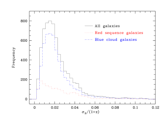
Figure 2: Distribution of relative redshift errors of galaxies with $I<23$, $M_{B}<-18$ and $0.4<z<0.8$ (solid line). Also shown are the redshift error distributions for red sequence and blue cloud galaxies.

3 The halo model of galaxy clustering

In discussing the results of clustering analyses of the COMBO-17 data, we will make frequent comparisons with theoretical predictions. We therefore now summarise the framework used to carry out this modelling. This goes back to the paradigm introduced by White & Rees (1978): galaxies form through the cooling of baryonic material in virialized haloes of dark matter. The mass function and density profiles of these haloes can be expressed in terms of simple fitting formulae derived from N-body simulations, and the large-scale clustering of haloes can be derived analytically for Gaussian density fields. This concentration on dark-matter haloes gives concrete form to earlier work on the clustering statistics generated by distributions of extended clumps (see e.g. Neyman & Scott 1952 and Scherrer & Bertschinger 1991).

With an accurate description of dark-matter clustering to hand, the stage was set for an extension to galaxies via the ‘halo model’ (Ma & Fry 2000; Seljak 2000; Peacock & Smith 2000; Cooray & Sheth 2002). In this picture, the key remaining uncertainty is the way in which galaxies occupy the dark matter haloes; this can be regarded as an unknown function, to be probed experimentally. The halo model then allows a simple and direct understanding of many features of galaxy clustering, and how the clustering of galaxies differs from that of the mass.

In this approach, the density field is a superposition of dark-matter haloes, with small-scale clustering arising from neighbours in the same halo. The corresponding real-space correlation function can be written as a combination of two parts:

$$\xi_{r}=\xi_{\rm lin}+\xi_{\rm halo}\leavevmode\nobreak\ ,$$ (5)

the first term representing the clustering of the dark matter haloes, and the second correlations from within a single halo. Large-scale halo correlations depend on mass, and the linear bias parameter for a given class of haloes, $b(M)$, depends on the rareness of the fluctuation and the rms of the underlying field (Kaiser 1984; Cole & Kaiser 1989; Mo & White 1996; Sheth & Tormen 1999), usually measured in spheres of $8{\,h^{-1}\,\rm Mpc}$ and termed $\sigma_{8}$. The mass profile of the haloes is known from simulations, and may be assumed to follow either an NFW profile (Navarro et al. 1996, 1997, 2004), or a Moore et al. (1999) profile.

The key feature that allows bias to be included is to encode all the complications of galaxy formation via an halo occupation number: the number of galaxies found above some luminosity threshold in a virialized halo of a given mass $M$. A simple but instructive model for this halo occupation distribution (HOD) is

$$N(M)=\cases{0\quad&($M<M_{c}$)\cr(M/M_{c})^{\alpha}\quad&($M>M_{c}$)\leavevmode\nobreak\ .\cr}$$ (6)

This is closely related to the mass-dependent weight introduced by Jing et al. (1998). A model in which light traces mass exactly would have $M_{c}\rightarrow 0$ and $\alpha=1$. The galaxies are assumed to be split into a central galaxy plus some number of satellite galaxies, which follow the mass distribution in the halo. It is necessary to make an assumption about the statistics of the HOD – in particular whether $N$ is a causal function of $M$ or whether it obeys a Poisson distribution. It is known that sensible results require sub-Poisson behaviour, and we assume the extreme limit in which $N$ is perfectly determined by $M$. Putting all these ingredients together, the galaxy correlation function can be calculated analytically.

Since its initial development, the halo model has been applied successfully to the interpretation of the correlation function of galaxies in the local universe, notably by Zehavi et al. (2004), who detected an inflection in the correlation function of SDSS red galaxies, interpreting it as indicating the transition regime between clustering dominated by 1-halo and 2-halo terms. The occupation model has been elaborated quite significantly (e.g. Abazajian et al. 2005; Zheng et al. 2005; Kravtsov et al. 2004; Tasitsiomi et al. 2004; Zentner et al. 2005), including up to three parameters for the occupation distribution, plus the inclusion of some nonlinear evolution of the power spectrum in the $\xi_{\rm lin}$ term. These sophistications can improve the detailed fit to correlation-function data from simulations, but they do run somewhat counter to the original heuristic spirit of the model. In this work, we shall retain the original method of calculation, as described in detail by Peacock & Smith (2000), together with the simple power-law occupation model. This approach seems justifiable in a first exploration of intermediate-redshift clustering, and the main features of interest are in any case relatively robust.

The form of any transition-regime feature in the correlation function depends mainly on the mean halo mass occupied by the galaxies, – i.e. the average value of $M$, weighted by $N(M)$ – and is insensitive to the details of their distribution within the halo. This typical halo mass is determined by our two-parameter model for $N(M)$ plus the halo mass function. We shall use the additional constraint of the observed number density of galaxies under study, so that there remains a single free parameter in the model – which we take to be the occupation slope $\alpha$. For a given value of $\alpha$, the number density determines the cutoff mass and hence the average halo mass. Different models of the HOD can of course be used; Zehavi et al. (2004) take $N=1$ above $M_{c}$ to represent central galaxies, plus a power-law $N(M)$ representing satellites, which commences at a mass of approximately $20M_{c}$ with a slope of $\alpha\simeq 1$. In practice, this model gives results similar to the single power law with $\alpha\simeq 0.6$, showing that the detailed shape of the HOD is hard to measure given only correlation-function data. The typical number-weighted halo mass is a more robust quantity, and this is probably the best way to compare different HOD models.

We will normally assume a standard flat cosmology with $\Omega_{m}=0.25$, $\Omega_{b}=0.045$ and $h=0.73$ where $H_{0}=100h$ km s^-1 Mpc^-1 (Spergel et al. 2006; Cole et al. 2005). The most uncertain cosmological parameter is the normalization of the power spectrum, $\sigma_{8}$. We will often assume a standard value of $\sigma_{8}=0.9$, but it is also of interest to leave both $\sigma_{8}$ and the power-law index $\alpha$ of the halo occupation number (equation 6) as free parameters, and determine them from a fit to the measured galaxy correlation functions.

4 Redshift space correlations

4.1 Projected correlations

With a sample of the present size, only the two-point correlation function, $\xi(r)$, can be determined accurately. Even this is not straightforward, because of the need to work in redshift space. While it is possible to measure angular positions on the sky with high precision, peculiar velocities as well as redshift errors distort the galaxy pattern along the line of sight, making $\xi({\bf r})$ appear anisotropic, and tending to reduce its amplitude.

These problems can be overcome by splitting the separation vector ${\bf r}$ of a pair of objects into components lying on the plane of sky, $r_{p}$, and along the line of sight, $\pi$, and compute the correlation function $\xi(r_{p},\pi)$ as a function of these two components. Projecting $\xi(r_{p},\pi)$ onto the $r_{p}$ axis gives the projected function $w(r_{p})$, which is independent of any radial distortions (Davis & Peebles 1983). For small angles $r^{2}=r_{p}^{2}+\pi^{2}$. Thus the projected correlation function is defined as

$$w(r_{p}) = \int_{-\infty}^{\infty}{\xi\left[(r_{p}^{2}+\pi^{2})^{1/2}\right]\leavevmode\nobreak\ {\mathrm{d}}\pi}$$ (7)

$$= 2\int_{r_{p}}^{\infty}{\xi(r)(r^{2}-r_{p}^{2})^{-1/2}\,r\leavevmode\nobreak\ {\mathrm{d}}r}\leavevmode\nobreak\ .$$

Note that $w(r_{p})$ has dimensions of length. Since the correlation function converges rapidly to zero with increasing pair separation, the integration limits do not have to be $\pm\infty$, but they have to be large enough to include all correlated pairs. As will be explained in the following paragraph, this is a crucial point when the redshift errors are large.

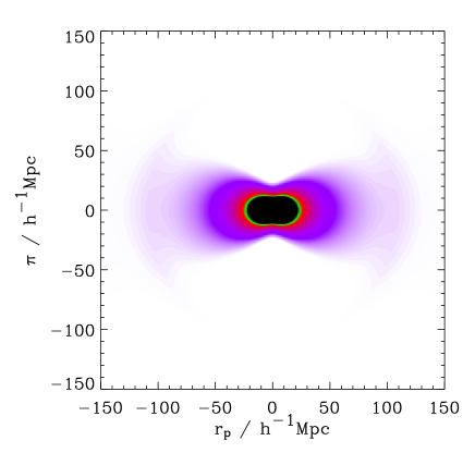
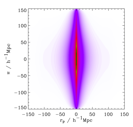
Figure 3: The redshift-space correlation function $\xi(r_{p},\pi)$ calculated using the halo model, plotted as a function of transverse ($r_{p}$) and radial ($\pi$) pair separation. The data from the first quadrant are repeated with reflection in both axes, in order to clarify deviations from isotropy. Upper panel: before convolution with the pairwise redshift error distribution inferred from the sample of COMBO-17 galaxies under consideration in this analysis, lower panel: after convolution.

4.2 The effect of redshift errors on $\xi(r_{p},\pi)$

We now illustrate the effects of redshift errors, starting from a model for the true $\xi(r_{p},\pi)$. This is calculated using the halo model, as described above in section 3, together with a prescription for redshift-space distortions. Seljak (2001) showed how to include redshift-space distortions in the halo model, but it is also common to use the following simple model for the ratio of redshift-space power to real-space power:

$$P_{s}/P_{r}={(1+\beta\mu^{2})^{2}\over(1+k^{2}\mu^{2}\sigma_{p}^{2}/2)},$$ (8)

where $\sigma_{p}$ is an effective pairwise velocity dispersion, $\mu$ is cosine of the angle between $\bf k$ and the line of sight, and $\beta\equiv\Omega_{m}^{0.6}/b$ (e.g. Ballinger, Peacock & Heavens 1996). This approach has the advantage that the redshift-space correlation function can then be found analytically, apart from a radial convolution (Hamilton 1992). We used this prescription, taking $\sigma_{p}$ to be $\sqrt{2}$ times the one-dimensional velocity dispersion calculated from the halo model. Fig. 3 shows a model $\xi(r_{p},\pi)$, which contains two well-known expected anisotropies: the isocorrelation contours of $\xi(r_{p},\pi)$ are stretched along the $\pi$ direction at small separations, because of the effect of virialized velocity dispersions, and compressed at large scales as a consequence of large-scale coherent motions. The former effect is not clearly visible owing to the large scale of the plot.

The effect of redshift errors on this redshift-space correlation function is straightforward: it is a convolution in the radial direction. This reflects the fact that $1+\xi$ is a ratio of the observed and expected numbers of pairs of galaxies. The correlation function $\xi(r_{p},\pi)$ becomes distributed more broadly along the $\pi$ axis, but the total correlation signal is conserved – this is why $w(r_{p})$ is independent of redshift errors. In order to model this process, we need a model for the convolving function. This is simply deduced, because the classification scheme automatically returns an estimate of the rms redshift error for each galaxy (see Wolf et al. 2004). Thus, given a pair of galaxies $i$, $j$, with redshift errors $\sigma_{z_{i}}$ and $\sigma_{z_{j}}$ the rms pairwise error is $\sigma_{{\rm pair}_{i,j}}=\smash{(\sigma_{z_{i}}^{2}+\sigma_{z_{j}}^{2})^{1/2}}$. The signal from this pair is smeared by a Gaussian with this width, so the overall convolving function is a sum of the Gaussians corresponding to all pairs:

$$f(\delta z)=\frac{1}{N}\sum_{\rm pairs}(2\pi\sigma_{\rm pair})^{-1/2}\exp\left[-(\delta z/\sigma_{{\rm pair},n})^{2}/2\right]\leavevmode\nobreak\ ,$$ (9)

where $N$ is the number of pairs $(i,j)$. After having transferred the pairwise redshift error distribution into comoving distances we can convolve $\xi(r_{p},\pi)$ with Eq. (9).

The effect of this convolution is shown in the second panel in Fig. 3. The redshift-space correlations are now heavily elongated in the radial direction, and some care is needed in extracting the projected correlation signal.

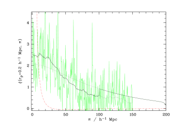
Figure 4: An example of the model-fitting procedure used to determine $w(r_{p})$: The grey line shows the correlation function $\xi(r_{p},\pi)$ of the red sequence galaxies as a function of $\pi$ at $r_{p}=0.2{\,h^{-1}\,\rm Mpc}$. The dashed line shows the model correlation function in the absence of redshift errors. The dotted and solid lines show the smoothed data (the smoothing was done by applying a box filter of length $40{\,h^{-1}\,\rm Mpc}$ along the $\pi$-axis using the running average), and the model after the convolution with the expected error distribution, with the solid part indicating where the integration is carried out.

4.3 Estimation of projected correlations

The simplest strategy for carrying out the projection needed in order to deduce $w(r_{p})$ would be to integrate $\xi(r_{p},\pi)$ over a very large radial range. Fig. 3 suggests that a maximum $\pi$ value of $150$ to $200{\,h^{-1}\,\rm Mpc}$ would be required to capture all the signal. The problem with this strategy is that the random noise in $\xi(r_{p},\pi)$ is independent of $\pi$ at a given $r_{p}$ (because the expected pair counts have a cylindrical dependence $\propto r_{p}\,dr_{p}\,d\pi$). Thus, integration to $\pi=200{\,h^{-1}\,\rm Mpc}$ would yield a random error in $w(r_{p})$ that is $\sqrt{2}$ times larger than integration to $\pi=100{\,h^{-1}\,\rm Mpc}$ – but the lower limit systematically misses part of the signal.

We have developed a strategy for solving this problem, which depends weakly on some prior knowledge of the likely form of the true clustering signal (after error convolution). A model for $\xi(r_{p},\pi)$ defines how the real-space signal $w(r_{p})$ is spread out in $\pi$; we are only concerned with the shape of this function, which is dominated by the convolution with the redshift error distribution. Given this probability distribution in the $\pi$ direction, the amplitude of $w(r_{p})$ can be estimated by fitting a scaled version of our model $\xi(r_{p},\pi)$ to the data at the $r_{p}$ value of interest.

In practice, our model $\xi(r_{p},\pi)$ will not be exact, and we considered the following compromise procedure for estimating $w(r_{p})$ so that the result is robust. For each $r_{p}$ value, we fit the amplitude of the (convolved) model $\xi(r_{p}={\rm const},\pi)$ to the data. We then integrate the data for $\xi(r_{p},\pi)$ out to $\pi=100{\,h^{-1}\,\rm Mpc}$, from which point on we integrate the convolved model out to infinity (see Fig. 4). This combines the exact measurement of $w(r_{p})$ within $\pi_{\rm max}=100{\,h^{-1}\,\rm Mpc}$ with an estimate of the missing signal at larger $\pi$. Since this correction is typically 20% of the overall signal, we do not need to estimate it very accurately. In practice, the results from the 2-stage procedure were very similar to the direct fitting method. This process is performed separately for the red and blue galaxy samples, using the appropriate pairwise error distributions and the final best-fitting halo-model $\xi(r_{p},\pi)$ for the unconvolved prediction.

The width of the convolved model in Fig. 4 suggests that the redshift errors yielded by the object classification scheme, which we used for the calculation of the pairwise error distribution, may be slightly overestimated. In order to estimate the effect on the projected correlation function, we tried repeating the analysis with redshift errors scaled to $80$% of the values given in the object catalogues. This scaling gives the best fit to the data; however, the resulting changes to $w(r_{p})$ were small compared to the random errors.

4.4 Integral constraint

The mean galaxy density is determined from the observed galaxy counts in each field, which does not necessarily represent the the true density (Groth & Peebles 1977). The estimator will be on average biased low with respect to the true correlation by a constant ${\cal I}$:

$$w_{m}(r_{p})=w_{t}(r_{p})-{\cal I}\leavevmode\nobreak\ ,$$ (10)

where $w_{t}(r_{p})$ is the true projected correlation function, $w_{m}(r_{p})$ the measurement. The integral constraint ${\cal I}$ is given by

$${\cal I}\simeq\frac{1}{S^{2}}\int{w_{\rm t}(r_{p})\mathrm{d}^{2}S_{1}\mathrm{d}^{2}S_{2}}\leavevmode\nobreak\ ,$$ (11)

where $S$ is the physical area corresponding to the solid angle of the field at the redshift under consideration. For the calculation of the integral constraint, we assume that the three dimensional correlation function $\xi(r)$ is to first approximation a power law:

$$\xi(r)=\left(\frac{r}{r_{0}}\right)^{-\gamma}\leavevmode\nobreak\ .$$ (12)

Then the evaluation of equation 7 yields

$$w(r_{p})=Cr_{0}^{\gamma}r_{p}^{1-\gamma}\leavevmode\nobreak\ ,$$ (13)

where $C$ is a numerical factor, which depends only on the slope $\gamma$:

$$C=\sqrt{\pi}\;\frac{\Gamma((\gamma-1)/2)}{\Gamma(\gamma/2)}\leavevmode\nobreak\ .$$ (14)

If the true correlation function is given by equation (13), the measurement yields

$$w_{m}(r_{p}) = Cr_{0}^{\gamma}r_{p}^{1-\gamma}-{\cal I}$$ (15)

$$= Cr_{0}^{\gamma}\left[r_{p}^{1-\gamma}-{\cal I}/(Cr_{0}^{\gamma})\right]\leavevmode\nobreak\ .$$ (16)

The true amplitude $Cr_{0}^{\gamma}$ is not known, but ${\cal I}/(Cr_{0}^{\gamma})$ can be estimated by performing a Monte Carlo integration (where we use the mean of the pair counts $\langle RR\rangle$ at a projected distance $r_{p}$ of the four fields):

$$\frac{{\cal I}}{Cr_{0}^{\gamma}}=\frac{\sum{\left[\langle RR\rangle\cdot r_{p}^{1-\gamma}\right]}}{\sum{\langle RR\rangle}}\leavevmode\nobreak\ .$$ (17)

The true value of $Cr_{0}^{\gamma}$ can be estimated by fitting equation (16) to the data, taking the value of ${\cal I}/(Cr_{0}^{\gamma})$ from equation (17). This value, multiplied by the fitted amplitude $Cr_{0}^{\gamma}$, yields the integral constraint ${\cal I}$. The measurement can then be corrected for the integral constraint by adding ${\cal I}$ to $w_{m}(r_{p})$.

This method yields estimates of ${\cal I}=0.14{\,h^{-1}\,\rm Mpc}$ for the red galaxies and ${\cal I}=0.33{\,h^{-1}\,\rm Mpc}$ for the blue galaxies. These values are negligible in comparison with the observed data for $r_{p}\la 20{\,h^{-1}\,\rm Mpc}$, demonstrating that the fields are large enough to deliver a fair sample. As a cross-check, note that we expect ${\cal I}=200\sigma^{2}$ (since we integrated over $\Delta\pi=200{\,h^{-1}\,\rm Mpc}$), where $\sigma^{2}$ is the fractional variance in galaxy numbers between different realizations of our survey. With three fields, $\sigma$ should be $\sqrt{3}$ times smaller than the field-to-field rms variation, so our figures for ${\cal I}$ suggest 4.5% and 7% expected scatter in the numbers of galaxies per field for red and blue galaxies respectively. This agrees well with the numbers in Table 1.

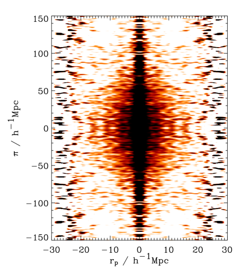
Figure 5: $\xi(r_{p},\pi)$ of all COMBO-17 galaxies with $0.4<z<0.8$, $I_{815}<23$ and $M_{B}<-18$. Again the data from the first quadrant are repeated with reflection in both axes. In the transverse direction the pair separations accessible for the analysis are limited by the COMBO-17 field of view.

4.5 Error analysis

Finally, there is the crucial issue of setting realistic error bars on our correlation estimates. The three COMBO-17 fields measure $\sim 31^{\prime}\times 30^{\prime}$ each and are thus large enough to carry out a jack-knife analysis. We divide each field into four quadrants, and then calculate the correlation function $w(r_{p})$ (including the integral constraint) for twelve realisations of the data, each time omitting one of the quadrants. The variance in $w$ is then given approximately by

$$\sigma^{2}=\frac{N-1}{N}\sum_{i=1,N}\left[\langle w(r_{p})\rangle-w_{i}(r_{p})\right]^{2}\leavevmode\nobreak\ ,$$ (18)

where $N=12$ is the number of realisations of the data (e.g. Scranton et al. 2002).

In order to check for cross-correlations between the data points, we can extend the jack-knife method in the obvious way to estimate the covariance between different bins, $\sigma^{2}_{ij}$. The natural way to express this is as a correlation coefficient matrix: $r_{ij}\equiv\sigma^{2}_{ij}/\sigma_{i}\sigma_{j}$. Results in this form are presented below.

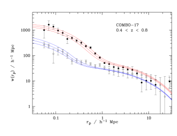
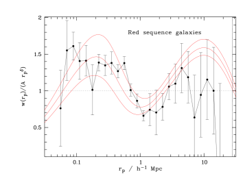
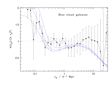
Figure 6: The projected correlation function $w(r_{p})$ for the COMBO-17 data, divided into red and blue galaxies. The lines show predictions from the halo model with $\alpha=0.45,0.5,0.55$ for red sequence and $\alpha=0.15,0.2,0.25$ for blue cloud galaxies, respectively, where increasing $\alpha$ corresponds to increasing clustering. The lower panels show an expanded view of the data, divided by the best-fitting power law (fitted in the range $\log_{10}r_{p}<1.1$).

5 The clustering of the COMBO-17 galaxies

5.1 Results

We calculated $\xi(r_{p},\pi)$ for all COMBO-17 galaxies in the redshift range $0.4<z<0.8$ with $I$-band magnitudes $I<23$ and absolute restframe $B$ band luminosities $M_{B}<-18$. We used the estimator invented by Landy & Szalay (1993). An angular mask for the survey was derived by censoring the surroundings of bright stars in the fields. The same mask was applied to a random catalogue consisting of $30\,000$ randomly distributed galaxies, each of which was assigned a redshift taken randomly from the real data, where the three fields were put together in order to smooth the redshift distribution. Using a smoothed form of the empirical redshift distribution did not yield a significant change in the results.

The resulting $\xi(r_{p},\pi)$ is shown in Fig. 5. The field of view of the COMBO-17 fields limits the pair separations accessible for the analysis, so in the transverse direction there is of course no signal at separations larger than the physical distance corresponding to the diagonal diameter of the fields.

For each object, we have an estimate of the redshift and the restframe colours and luminosities; it is therefore possible to divide the sample into two distinct colour classes as described earlier. For both samples we calculated $w(r_{p})$ as described in section 4, correcting for the integral constraint ${\cal I}$, and the influence of the redshift errors. These results are shown in Fig. 6.

5.2 Fitting the halo model

Fig. 6 also shows predictions from the halo model, varying the single occupation-number parameter $\alpha$, and choosing the cutoff $M_{c}$ so as to match the observed comoving densities of $0.004h^{3}{\rm Mpc}^{-3}$ (red) and $0.012h^{3}{\rm Mpc}^{-3}$ (blue). It is apparent that there is greater sensitivity to $\alpha$ at small separations, and that once $\alpha$ is fixed from the data there, there is little freedom at large separations, where the data and the model match satisfyingly well. The preferred values are approximately $\alpha=0.5$ for the red population and $\alpha=0.2$ for blue galaxies. These figures correspond to cutoff masses of respectively $M_{c}=10^{12.15}h^{-1}M_{\odot}$ and $M_{c}=10^{11.50}h^{-1}M_{\odot}$. As discussed earlier, a more meaningful way of casting these numbers may be to apply the HOD model to the halo mass function, to calculate the effective halo mass, weighting by galaxy number. These figures come out as $M_{\rm eff}=10^{13.21}h^{-1}M_{\odot}$ and $M_{\rm eff}=10^{12.52}h^{-1}M_{\odot}$ respectively.

Fig. 6 also shows a magnified view, with the measured correlation functions and the corresponding best-fitting models both divided by a power-law fit (fitted in the range $\log_{10}r_{p}<1.1$), the slope and amplitudes of which are given in Table 2. The data points do not scatter arbitrarily around the power-law fit, but show systematic deviations. For the red galaxies, there is a marked dip around $r_{p}\simeq 1.5{\,h^{-1}\,\rm Mpc}$; the blue galaxies are closer to a power law, but with a relatively abrupt step at $r_{p}\simeq 0.2{\,h^{-1}\,\rm Mpc}$. Both these features are impressively well accounted for by the halo model predictions, especially when it is considered that there is only one free parameter.

Table 2: The amplitudes, slopes and resulting correlation lengths $r_{0}$ of the best fitting power law ($w(r_{p})=Ar_{p}^{\delta}$, fitted for $\log_{10}r_{p}<1.1$), for the total sample, and divided into red sequence and blue cloud galaxies.

$A_{\rm tot}$	$\delta_{\rm tot}$	$r_{0}^{\rm tot}$
$53.98\pm^{3.86}_{3.50}$	$-0.57\pm 0.02$	$4.71\pm^{0.26}_{0.26}$
$A_{\rm red}$	$\delta_{\rm red}$	$r_{0}^{\rm red}$
$86.28\pm^{4.86}_{4.50}$	$-0.94\pm 0.03$	$5.39\pm^{0.30}_{0.28}$
$A_{\rm blue}$	$\delta_{\rm blue}$	$r_{0}^{\rm blue}$
$37.09\pm^{2.58}_{2.41}$	$-0.45\pm 0.03$	$3.64\pm^{0.25}_{0.24}$

It is interesting to compare our results with those of the VVDS project (Le Fèvre et al. 2005). They give results to a similar depth for two fields, although not divided by colour, with a total of 7155 redshifts over 0.61 deg². Their redshift bins are not identical, but they quote $r_{0}=2.69^{+0.53}_{-0.59}{\,h^{-1}\,\rm Mpc}$ and $\gamma=1.71^{+0.18}_{-0.11}$ at $\langle z\rangle=0.6$ and $r_{0}=4.55^{+1.25}_{-1.56}{\,h^{-1}\,\rm Mpc}$ and $\gamma=1.48^{+0.28}_{-0.15}$ at $\langle z\rangle=0.7$. The latter figure is from the CDFS, which is one of our fields, and we have checked that our figure for this field alone agrees well with the VVDS, as it does for our other fields. The VVDS $2^{h}$ field thus gives a somewhat lower clustering strength; this may be because the VVDS sample in that field is about 0.5 mag. deeper than the one studied here, plus the fact that the VVDS analysis has no lower limit in luminosity. The ratio in $r_{0}$ between the VVDS $2^{h}$ field and our overall result is $1.75\pm 0.21$, so a factor 1.3 from luminosity-dependent clustering would be required in order to make the results statistically consistent.

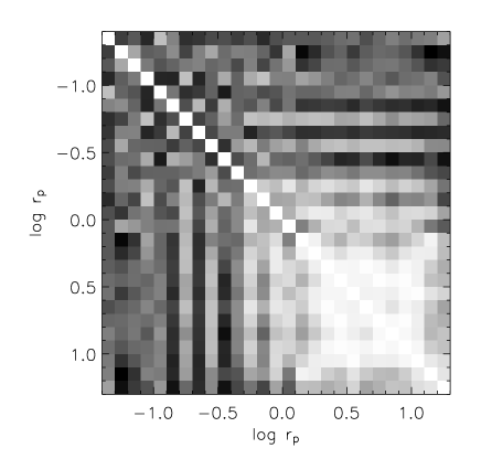
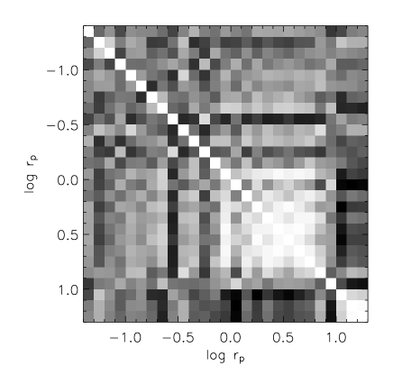
Figure 7: The correlation matrices for red (upper panel) and blue (lower panel) galaxies, for $-1.4<\log_{10}r_{p}<1.3$. The apparent strong correlation between the large scale data points (lower right corner) is due to the integral constraint.

Figure 8: The likelihood contours for the two free parameters $\alpha$ and $\sigma_{8}$. Upper panel: red galaxies; lower panel: blue galaxies. Contours are shown at the Gaussian equivalent of the following confidence levels: 68% 1-parameter, 68%, 95%, 99%, 99.9%, 99.99% 2-parameter, i.e. $\Delta\ln{\cal L}=0.5$, 1.1, 3.0, 4.6, 6.9, 9.2.

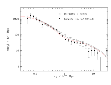
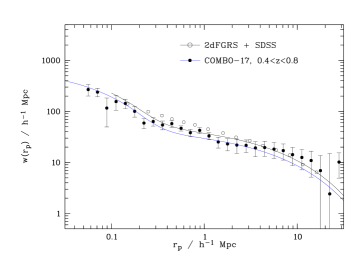
Figure 9: The projected correlation function in the redshift bin $0.4<z<0.8$ (filled circles) in comparison with the local data (open circles). The upper panel shows red sequence galaxies, the lower panel is for blue cloud galaxies. The lines show the prediction of the halo model, which are higher in the $z=0$ case.

Figure 10: The likelihood contours for the two free parameters $\alpha$ and $\sigma_{8}$, now fitting the $z=0$ data. Upper panel: red galaxies; lower panel: blue galaxies. Contours are shown at the Gaussian equivalent of the following confidence levels: 68% 1-parameter, 68%, 95%, 99%, 99.9%, 99.99% 2-parameter, i.e. $\Delta\ln{\cal L}=0.5$, 1.1, 3.0, 4.6, 6.9, 9.2.

We now want to quantify the agreement between model and data in more detail, using the jack-knife error estimates. This would be straightforward if the covariance matrix were diagonal, and if the model was exact. In practice, there is some degree of correlation in the data, and the simple halo model used here may be expected to have some systematic deviations with respect to ideal data. The correlation matrices in Fig. 7 indeed show a strong correlation between the large-scale data points (large matrix indices, lower right corner). This is due to the integral constraint, which is included in the calculation of the jack-knife realisations: all large-scale data points are offset by the same amount and thus become correlated. This issue is not too serious, since the errors in this regime are in any case large. We therefore ignore the large-scale points at $r_{p}>10{\,h^{-1}\,\rm Mpc}$ and treat the remaining data as independent. Even so, our approximate model is not guaranteed to deliver a perfect fit. In order to achieve a formally acceptable value of $\chi^{2}$ for the fit, we added in quadrature an error of 5% to the errors on $w$ for red galaxies. When fitting the $z=0$ data, as discussed below, a covariance matrix was not available, and the formal errors are in any case small. In this case, we therefore took what is effectively a least-square approach, which required an effective error of 10% in both blue and red galaxies.

In performing the fitting, it is interesting to consider variations in both the power-law index $\alpha$ of the HOD (equation 6), and in the normalization $\sigma_{8}$. We emphasise that $\sigma_{8}$ is the zero-redshift value, which is connected to the degree of inhomogeneity at $z=0.6$ by the growth factor predicted by the cosmological model (a change in linear density contrast by a factor 1.32). Fig. 8 shows the likelihood contours for these two free parameters $\alpha$ and $\sigma_{8}$. The preferred values and marginalized rms errors are $\alpha=0.56\pm 0.03$ and $\sigma_{8}=0.84\pm 0.08$ for the red sequence galaxies and $\alpha=0.16\pm 0.03$ and $\sigma_{8}=1.19\pm 0.09$ for the blue population.

These independent estimates of $\sigma_{8}$ from the red and blue populations are both close to our default value of 0.9. The agreement is not perfect, and the difference in $\sigma_{8}$ is formally $3\sigma$, but the mean value of $\sigma_{8}=1.02\pm 0.17$ is certainly plausible. Given the simplicity of the HOD model, this is a satisfying result.

5.3 Robustness of the results

In view of the tension between the normalization inferred from the red and blue galaxies, and in the light of the preference for a low normalization of $\sigma_{8}\simeq 0.75$ from the 3-year WMAP data (Spergel et al. 2006), it is important to discuss the extent to which our result is rendered uncertain by simplifying assumptions in the modelling.

The halo model is an idealized approximation in many ways, and one issue in particular has generated considerable discussion recently. It has been shown that the clustering of dark matter haloes is dependent on the halo formation time (Sheth & Tormen 2004a, b; Gao et al. 2005; Wechsler et al. 2005; Harker et al. 2006; Reed et al. 2006), and the question is what impact this has on halo model calculations. To some extent, the effect is already included in the halo-model formalism: when the cosmic density field is smoothed on a given mass scale, the clustering of peaks in the smoothed field is well known to increase with peak height, i.e. with formation redshift (Kaiser 1984). More massive systems are more strongly clustered for the same reason: only the rarest peaks exceed the threshold for collapse when the variance in filtered density is low. When we use the standard expression for bias as a function of mass, this averages over all systems that have collapsed by the present: the dependence of clustering on formation time will thus have no effect on predicted galaxy properties if the occupation numbers are purely a function of halo mass. However, it seems reasonable that the occupation number for a given mass will in fact depend to some extent on collapse redshift (e.g. more red galaxies in a halo that collapses early). At a minimum, the age-clustering effect will then contribute to a stochastic aspect of the occupation number, so that there is some scatter in $N$ at a given $M$. More seriously, it can also bias the mean clustering compared to all haloes of that mass. The influence of these effects on halo-model predictions remains to be explored, and this task is beyond the scope of the present paper. Some work along these lines has been done by Zentner et al. (2005) and by Croton, Gao & White (2006), where the halo contents in a simulation are scrambled between all haloes of the same mass, thus destroying any correlations with collapse redshift. Zentner et al. (2005) did this for subhaloes, but Croton, Gao & White (2006) considered the case of most direct interest, which is semianalytic galaxy populations. They do detect systematic shifts in correlation amplitude, but for the luminosities of interest here these are no larger than 10%. Such shifts are not important in comparison with the COMBO-17 measuring errors, but this is clearly an issue that should be looked at in more detail, especially as the accuracy in measuring high-redshift clustering improves.

Table 3: The inferred values of $\sigma_{8}$ from COMBO-17 red and blue galaxies, showing the effect of variations in some of the assumptions in the halo-model calculation. We also give the corresponding values of $\alpha$, the power-law slope in the occumaption model, plus formal values of $\chi^{2}$ for the best-fitting models (on 20 data points).

Halo Model	$\sigma_{8}^{\rm red}$	$\sigma_{8}^{\rm blue}$	$\alpha_{\rm red}$	$\alpha_{\rm blue}$	$\chi^{2}_{\rm red}$	$\chi^{2}_{\rm blue}$
Standard	0.84	1.19	0.56	0.16	26.2	09.7
$\Omega_{m}=0.2$	0.80	1.07	0.52	0.16	38.0	16.1
$h=0.6$	0.90	1.15	0.51	0.14	33.0	10.4
$1+\delta_{v}=300$	0.90	1.02	0.55	0.18	43.1	09.6
Zheng $N(M)$	0.85	0.98	0.96	0.56	46.4	09.4

Other degrees of freedom in the halo model are more easily investigated, and we summarise some tests here, the results of which are presented in Table 3. We show the impact on the values of $\sigma_{8}$ inferred from red and blue galaxies by (a) varying cosmological parameters; (b) varying parameters internal to the halo model; (c) varying the occupation number prescription. In the first category, we see that the Hubble parameter has very little effect, but that $\sigma_{8}$ increases with $\Omega_{m}$ very roughly as $\Omega_{m}^{0.3}$ to $\Omega_{m}^{0.5}$, with a larger sensitivity for the blue galaxies. In the second category, we considered altering the assumed density contrast for a virialized halo from the usual figure of 200 to a slightly larger number, which is sometimes assumed in a low-density model. Finally, we modify our simple power-law $N(M)$ to something that resembles more closely the prescription used by e.g. Zheng et al. (2005): $N=1$ between $M_{c}$ and $10M_{c}$, rising as $M^{\alpha}$ for smaller $M$ (we considered $\alpha\leq 1$). We also include the formal $\chi^{2}$ values for some of these alternatives. It appears that the standard model provides the best fit, especially to the red galaxies. However, bearing in mind the simplified nature of the halo model, these differences should not be given high weight; it is more interesting to concentrate on the robustness of the best-fitting parameters.

The overall conclusion of these tests is that plausible variations of some of the degrees of freedom in the modelling can alter $\sigma_{8}$ by 10 to 20%, and in a way that changes the consistency between red and blue results by a similar amount. We therefore conclude that the modelling is working as well as could have been expected, and that there is no need to be concerned by either the internal red-blue tension or by the 1.6$\sigma$ discrepancy with the WMAP $\sigma_{8}$. We now turn to the comparison with $z=0$; some of the systematics in the analysis should be common to all redshifts, so we should hope for a good level of consistency between measurements based on data from different epochs.

5.4 Comparison with local clustering

As a local comparison, we considered $w(r_{p})$ for a combined set of red and blue galaxies taken from both Sloan Digital Sky Survey (SDSS; York et al. 2000) and 2dFGRS (Colless et al. 2001) data. The sample has been divided into red and blue by either the bimodality of the rest-frame colour distribution, or spectral type, in a way that should compare reasonably well with the COMBO-17 classification. We use the flux-limited 2dFGRS results of Hawkins et al. (2003a), and the $-19>M_{r}>-20$ results of Zehavi et al. (2005), which have closely comparable amplitudes. Fig. 9 shows a comparison of the local and the high redshift sample. What is apparent here is that the main difference between the COMBO-17 sample at $z=0.6$ and the local data is in the shape of the correlation function, with almost identical amplitudes at small scales, but a difference of nearly a factor two for $r_{p}>1{\,h^{-1}\,\rm Mpc}$.

As shown in Fig. 9, the halo model is capable of accounting for these differences. Fig. 10 repeats the model-fitting exercise for the $z=0$ data, and the preferred values and marginalized rms errors are $\alpha=0.49\pm 0.02$ and $\sigma_{8}=1.03\pm 0.07$ for the red sequence galaxies and $\alpha=0.23\pm 0.02$ and $\sigma_{8}=1.00\pm 0.05$ for the blue population. These values of $\alpha$ are slightly smaller than those obtained from COMBO-17; they correspond to cutoff masses of respectively $M_{c}=10^{12.20}h^{-1}M_{\odot}$ and $M_{c}=10^{11.50}h^{-1}M_{\odot}$, or effective halo masses $M_{\rm eff}=10^{13.50}h^{-1}M_{\odot}$ and $M_{\rm eff}=10^{12.80}h^{-1}M_{\odot}$ respectively. Compared to the $z=0.6$ results, $M_{c}$ has not changed much, but $M_{\rm eff}$ has increased by about a factor 2. This makes sense in terms of hierarchical growth: the minimum dark-matter mass needed to assemble a galaxy-sized amount of baryons should be invariant, but such haloes inevitably merge into larger systems as time progresses.

The mean value of $\sigma_{8}=1.01\pm 0.04$ from the $z=0$ data agrees very well with $\sigma_{8}=1.02\pm 0.17$ from COMBO-17. This agreement assumes hierarchical growth in the halo mass function between $z=0.6$ and the present, without which the inferred values of $\sigma_{8}$ would have been expected to differ by a factor 1.3.

6 Summary & conclusions

Using a sample of 10  360 galaxies with photometric redshifts from the COMBO-17 survey, we have investigated in some detail the shape of the correlation function at redshift $\langle z\rangle\simeq 0.6$. We have shown for the first time that the two-point correlation functions of both red sequence galaxies and blue cloud galaxies at this redshift display deviations from a power law, analogous to the deviations seen at low redshift (Hawkins et al. 2003a; Zehavi et al. 2004).

We have compared these observations to the predictions of a simple halo model, and find a good fit. It appears that the COMBO-17 data allow us to identify the point of transition between 1-halo clustering and 2-halo clustering, as was done at $z=0$ by Zehavi et al. (2004). The implication is that the red and blue galaxies at $\langle z\rangle=0.6$ inhabit haloes of typical effective mass $M_{\rm eff}=10^{13.2}h^{-1}M_{\odot}$ and $M_{\rm eff}=10^{12.5}h^{-1}M_{\odot}$ respectively.

We have also allowed the zero-redshift normalization of the power spectrum, $\sigma_{8}$, to be a free parameter in this analysis. Impressively, both red and blue subsets imply a consistent local normalization of the power spectrum: $\sigma_{8}\simeq 1$. This figure is close to the value inferred by independent means using CMB and gravitational lensing (e.g. Refregier 2003), and certainly within the tolerance expected from the inevitable systematics associated with the simple modelling that we have used in this first analysis of galaxy clustering at intermediate redshifts. This consistency is obtained by assuming that the dark halo mass function grows in a standard hierarchical fashion so that the normalization at $z=0.6$ is approximately 30% lower than today. Our results amount to a verification that growth of this order has occurred.

We intend to expand this work to higher redshifts using COMBO-17+4, the NIR extension of COMBO-17, for which observations are currently being carried out using the $2k\times 2k$ Omega2000 camera at the 3.5m-telescope on Calar Alto, Spain. Combining the existing optical data base from COMBO-17 with NIR observations in one broad and three medium band filters (covering the wavelength range from 1040 to 1650 nm), we expect to obtain $\simeq 4200$ galaxy redshifts with an accuracy of $\sigma_{z}/(1+z)=0.02$ up to $z=2$. This much longer baseline in cosmic time will allow us to observe much larger evolution of halo masses, testing the idea of hierarchical growth back to a time close to the formation of luminous galaxies.