ION HEATING IN COLLISIONLESS SHOCKS IN SUPERNOVAE AND THE HELIOSPHERE Kelly Elizabeth Korreck Doctor of Philosophy Space and Planetary Physics 2005 Associate Professor Thomas H. Zurbuchen, Co-Chairperson
Dr. John C. Raymond, Co-Chairperson, Smithsonian Astrophysical Observatory
Professor August Evrard
Professor Lennard A. Fisk
Associate Professor Timothy A. McKay

$\copyright$        Kelly E. Korreck     2024 All Rights Reserved

For my past, present, and future.

ACKNOWLEDGEMENTS

I would like to thank Thomas Zurbuchen, my advisor for his belief in me and his willingness to take me on in my third year. I admire your drive and passion for all that you do.

I thank Dr. John C. Raymond who was my advisor for my year and a half that I spent at the Harvard-Smithsonian Center for Astrophysics. He is patient. His knowledge of the field is incredible. And he is a great mentor. I especially thank him for his enthusiasm for collaborating on and discussing the neutral code.

Of course, I am grateful to my parents for their patience and love. I have a very large extended family and I would like to thank them all for their support throughout all of my life. Grandpa Korreck, you are an inspiration to us all, 92 and still going strong! I think I get my natural curiosity and need to keep going from you!

To my best friend, my sister. Somehow we grew up and became friends. I know mom said it would happen but I remember times when I thought it never could. Thank you for your support and the endless shopping trips!

And to my little brother, who isn’t so little anymore. I know you love the Maize and Blue as much as I do. Do whatever your heart tells you and I know you will do it well!

And now my newest brother - well brother-in-law if you want to get technical. Mike, I am so happy you are part of our family. I hope you enjoy your copy of the thesis as you may be the only one besides me or my future grad students to read it!

The only way to get through grad school is with support of friends and family. I have been so lucky to have such wonderful friends and collaborators. The list is long and I apologize for anyone who I missed. Margaret Reid, Jan Beltran, Sue Griffith and all the AOSS staff - You have been there to listen to gripes and help workout the hard problems. Thank you so much! As part of the FUSE team, Ravi Sankrit helped with the night extraction of the FUSE data as well as fruitful conversations about shock physics and supernova remnants. Thanks also goes to Parviz Ghavamian for his advice, guidance, and ds9 skills.

Amy Reighard played sphere with me in the early years. She also kept me going and believing in myself when I was in doubt. Amy is an amazing physicist and I hope we can collaborate in the future.

The Empress Alysha, I will be the advisor for you anytime. Thank you for your help getting me through classes and the qualifiers. You are a great friend-just watch out for bears!

Pat Koehn for reading many chapters and the niffy template! I am so excited for you to start your teaching position. You just seem to be one of those who just has ’it’ when it comes to teaching!

Kevin Kane thanks for the support especially though the last few months! Thank you for lending me your house to finish the last two chapters of the thesis. And Lena Adams and all the women of AOSS you make the department wonderful!

A special thanks to my kitty Orion, who warmed my lap many a nights as I wrote this work.

Sue Lepri from my roommate to my officemate–I got though Jackson because of you. I enjoy working on everything from science projects or social affairs or hair cutting with you! And why does everyone say, ’Here comes trouble’ when they see us together? And of course to keep with tradition I must mention your funny faces that have entertained a generation of graduate students!

For Suni, my favorite! I am so happy that I get to come back to Cambridge for a while so we can go to the cider mill and hopefully learn how to sail! For Chelle Reno who always has a way with words and a zest for adventure of which I can only sit in amazement. I can’t thank you enough for coming into town to see my oral defense of this thesis. Hopefully we can all stick together through the years!

To My Cambridge Crew: Jim Carey, Raslyn Rendon, Dana Ozik(and Todd too), Jeno Soloski, Paul Martini, Matt Rosen, Matt Povich, Travis Metcalf, Maryam, Jenny Greene, Cara Rakowski and probably many more I have accidently forgotten. Working with you all is an amazing experience! I really enjoyed being a part of the CfA community and can’t wait to see what lies ahead!

Thank you to everyone who supported me in one way or another throughout this learning process. I am a better person for knowing you and going through the experience!

Ann Arbor, Michigan Kelly E. Korreck
May 2005

TABLE OF CONTENTS

toc

LIST OF FIGURES

lof

LIST OF TABLES

lot

Chapter I Introduction

Gazing into the night sky is a favorite pastime of the human race. The earliest human records have symbols of astronomical events and objects such as the moon and the Sun. The ancient Greeks saw many ”pictures” in the stars that are now known as constellations that rotate around the sky throughout the year. Each constellation had a story associated with it, mythical stories about heros, princesses, and creatures. Supernovae or ”guest stars” have been recorded by ancient Chinese astronomers (Strom, 1994). The native people of North America depended on the heavens to determine the best time for planting crops as well as for spiritual and religious rites. The Lakota, a nomadic people, used the equinoxes and solstices to track seasons for hunting and to prepare for their sacred spring ceremonies (Goodman, 1992).

Figure 1.1: The photograph above is the Aztec Calendar Stone, also called Sunstone. The carvings in the stone represent a rayed disk with the four previous cycles of creation and destruction. The skull at the center depicts the god Tonatiuh, the fifth Sun. Image courtesy of Corel Corporation.

The bright lights of the Aurora Borealis, sometimes referred to as the Northern Lights, have meant many things to ancient people. For the Fox Indians of Wisconsin, they were an omen of war (Finland, 1998). The lights were the ghosts of their slain enemies who sought revenge. We know today these lights are caused by cascading energetic particles from the Sun exciting emissions in the atmosphere. But for the Salteaus Indians of eastern Canada and the Kwakiutl and Tlingit of Southeastern Alaska the northern lights were the dancing of human spirits or animal spirits, especially those of deer, seals, salmon and beluga: the animals that gave them sustenance (Ray, 1958).

The Aztecs, of present day Mexico, believed in the Sun as an active living being, named Tonatiuh, pictured in Figure 1.1, that had a beginning and an end. A new Sun would replace the old. In order to keep the Sun strong they needed to make sacrifices to the Sun. Their temples and buildings were aligned with the sunrise and sunsets of the solstices to track the life of the current Sun(Universe, 2000).

The events unfolding in the heavens were viewed as powerful symbols and signs and those chosen few that interpreted them were considered high priests or magicians. Even today the popularity of Star Trek, Star Wars, and other science fiction allows us to feed our own curiosity about the cosmos. Humans have always felt very connected and as if they participated in what occurred in the cosmos.

Modern science has proven through remote and in situ observations that the cosmos is more mysterious and amazing than previously thought. But ”ordinary” in the sense that terrestrial physics applies to objects in space. Stars, including our Sun, and most of the objects in ”outer space” are in the fourth state of matter called a plasma. A plasma can be defined as ’a quasi-neutral gas of charged and neutral particles which exhibits collective behavior’(Chen, 1984). Quasi-neutral means that although the atoms in the plasma are ionized, there are equal number of electrons and positively charged ions. Their collective behavior allows the plasma to be described as a fluid instead of individual atoms or ions. The plasma can be characterized by fluid dynamics. One parameter often used when discussing magentic plasmas is the Alfvenic speed. The Alfvenic speed is the speed that magnetic information travels in the plasma.

$$v_{A}=\frac{B}{\sqrt{\rho\mu_{o}}}$$ (1.1)

One interesting aspect of fluid dynamics is the steepening of waves into shocks. These shocks create a difference in density, velocity, and thermal energy between regions of the plasma and are important in the study of astrophysical systems.

1.1 Collisionless Shocks in Astrophysical Plasmas

If a disturbance propagates through a plasma faster than the characteristic or Alfvenic speed of the local plasma, a shock is formed. Qualitatively, this is similar to the formation of a sonic boom or water waves breaking close to the beach.

In general, shocks transfer energy and momentum through the collision of atoms or molecules. However, most space-based shocks are collisionless. A collisionless shock occurs when the characteristic shock length is much smaller than the collisional mean free path of the particles in the plasma. Collisionless shocks were confirmed by the discovery and study of the Earth, Heliosphere, and solar wind in the late 1960’s (Sonett and Abrams, 1963; Kennel et al., 1985). These shocks transfer energy and momentum via electromagnetic and wave interactions and not collisions. Collisionless shocks appear in many different physical systems such as those produced by Coronal Mass Ejections (CMEs) in the Heliosphere, the termination shock, new stars (Herbig-Haro objects), jets from Active Galactic Nuclei (AGN), and supernova remnants.

Collisionless shocks have been studied for several decades but are still not well understood. There are several questions that remain to be answered about collisionless shock physics (Lembege et al., 2004). They include the electron heating and dynamics at the collisionless shock front, the particle diffusion via turbulence, electric, and magnetic fields, general particle acceleration by these shocks and pickup ions interaction with the collisionless shocks. Pickup ions are atoms from the Interstellar Medium (ISM) which are ionized by solar radiation and then carried along with the solar wind.

This thesis will address the heating and acceleration mechanisms at collisionless shocks fronts and the differences in heating observed for various ion species. Observed ion heating thus far have shown that the heating ”fractionates” according to the mass or charge of a particle. Ion heating creates a thermal seed population necessary to accelerate ions to higher cosmic ray energies. Several outstanding questions are -

What is the heating mechanism responsible for the fractionation of the ions?

Why does the heating process fractionate the ions according to mass?

How does the mass fractionation of the heating process affect the seed population?

To cover a wide range of parameter space in investigating these heating questions, two very different shock systems were used: the heliospheric shocks that occur in front of CMEs and the shocks of a supernova remnant, SN1006. Heliospheric shocks, including the bow shock, have been studied as the acceleration mechanisms for ions. Supernova remnants are also known to be the most powerful particle accelerators which produce high energy cosmic rays. The heliospheric shocks represent lower velocity shocks and lower Mach number shocks, with v_shock less than 1000 km s^-1 and M_A$\sim$ 1-5. The SN1006 shock represents the faster velocity and higher Mach shocks at v_shock $\sim$ 3000 km s^-1 and M_A$\sim$100. However, shock properties are fundamental in nature and thus can be related by scaling or a specific physical parameter.

For a greater understanding of the ion heating that is implicit to the acceleration method, a comparison study of the conditions of shocks and the heating mechanisms are necessary. Bulk thermalization of the kinetic energy of the shock would be the simplest heat transfer method; however, work done in the heliosphere indicates a different form of heating dominates.

Heliospheric shocks have been studied in much detail because of the availability of in situ data. Initial analysis of data from various satellites showed a mass proportional heating. Ogilvie et al. (1980) used particle distribution data from the ISEE3 satellite to analyze helium (He²⁺) and oxygen( O⁷⁺) in the solar wind. Although the accuracy of the data for heavier ions (oxygen) data were poor, the average heating was approximately mass proportional. Any heating was attributed to wave interaction close to the Sun, rather than shock heating.

Studies using the Prognoz satellite at 1 AU by Zertsalov et al. (1976) found heating less than mass proportional for Helium. Berdichevsky et al. (1997) studied the heating of ions in interplanetary shocks. This work contradicts the earlier work on shock heating and showed a greater than mass proportional heating present in the shocks for helium and oxygen ions. These shocks heated oxygen ions 19 - 48 times more than the protons, such that the heating is 1.2 to 3.0 times mass proportional. These same shocks heated helium 4.6 - 10.8 times more than the protons. The heating of the helium was 1.2 - 2.7 times more than mass proportional.

Supernovae interact with the ISM based on the nature of the progenitor star and the make up of the medium surrounding the specific supernova. Study of these collisionless shocks must explore the interaction and subsequent heating produced by the shock with ions heavier than protons as well as the shock-neutral ISM interaction. Past measurements of ion heating (Korreck et al., 2004; Ghavamian et al., 2002), electron (Laming et al., 1996), proton and ion temperature, and other emission features are studied to understand both the supernova explosion and the interstellar medium into which the shocks are expanding. Studies to date have shown a less than mass proportional heating for supernova shocks (Korreck et al., 2004; Raymond et al., 1995). This directly contradicts what is found for the heliospheric shocks and leads to questions about the injection process necessary for cosmic ray acceleration, such as how the mass of the ion species plays a role in the heating mechanisms.

In order to understand shock heating, a definition of several plasma and shock characteristics is necessary. A shock most generally is a transition layer which propagates through a plasma causing discontinuous changes in the density, velocity, and pressure of the plasma (Tidman, 1969). If a magnetic field is present, the plasma can be described by the Magnetohydrodynamics (MHD) equations for mass, momentum and energy conservation. From Gombosi (1999), the following are the conservative form of the ideal MHD equations in 3-D shown below, assuming no external forces (i.e. gravity):

Conservation of Mass:

$$\frac{\partial\rho}{\partial t}+\nabla\cdot(\rho\vec{u})=0$$ (1.2)

Conservation of Momentum:

$$\frac{\partial(\rho\vec{u})}{\partial t}+\nabla\cdot(\rho\vec{u}\vec{u}+p\vec{I}+\frac{B^{2}}{2\mu_{0}}\vec{I}-\frac{\vec{B}\vec{B}}{\mu_{0}})=0$$ (1.3)

Conservation of Energy:

$$\frac{\partial}{\partial t}(\frac{1}{2}\rho u^{2}+\frac{1}{\gamma-1}p+\frac{B^{2}}{2\mu_{0}})+\nabla\cdot(\frac{1}{2}\rho u^{2}\vec{u}+\frac{\gamma}{\gamma-1}p\vec{u}+\frac{(\vec{B}\cdot\vec{B}\vec{u}-\vec{B}(\vec{B}\cdot\vec{u}))}{\mu_{0}})=0$$ (1.4)

Induction Equation:

$$\frac{\partial\vec{B}}{\partial t}=\nabla\times(\vec{u}\times\vec{B})$$ (1.5)

Lack of Magnetic Monopoles:

$$\nabla\cdot\vec{B}=0$$ (1.6)

where
$\rho$=mass density
$\vec{u}$= flow velocity
p=thermal pressure
$\vec{B}$=magnetic field B= magnitude of the magnetic field
B_n=normal component of the magnetic field
B_t=tangential component of the magnetic field
$\vec{I}$=Identity matrix
$\mu_{0}$=permeability of free space
$\gamma$=adiabatic index

The MHD equations characterize the plasma as a fluid but do not predict the shock conditions. Three characteristic waves can develop in the plasma described by the MHD equations and steepen into shock waves or discontinuities. These waves are named according to their speed: slow, intermediate, and fast waves. Each wave is related to the Alfven speed and the angle between the shock normal and the magnetic field.

If the discontinuity of the shock is considered infinitesimally thin, the fluxes of the mass, momentum, and energy should be conserved across the discontinuity. The Rankine-Hugoniot relations, Equations 1.7-1.12, describe the relationship between pre-shock to post-shock physical characteristics due to conservation of mass flux, momentum, and energy across the shock front.

From the continuity equation:

$$[\rho u_{n}]=0$$ (1.7)

From the conservation of momentum equation:

$$[\rho u_{n}\vec{u_{t}}-\frac{B_{n}\vec{B_{t}}}{\mu_{0}}]=0$$ (1.8)

From the conservation of energy flux equations:

$$[\rho u_{n}^{2}+p+\frac{B_{t}^{2}-B_{n}^{2}}{2\mu_{0}}]=0$$ (1.9)

$$[\frac{1}{2}\rho(u_{n}^{2}+u_{t}^{2})u_{n}+\frac{\gamma}{\gamma-1}pu_{n}+\frac{B_{t}^{2}}{\mu_{0}}u_{n}-\frac{B_{n}}{\mu_{0}}(\vec{B_{t}}\cdot\vec{u_{t}})]=0$$ (1.10)

In addition from the induction and magnetic monopole equations we have:

$$[u_{n}\vec{B_{t}}-B_{n}\vec{u_{t}}]=0$$ (1.11)

$$[B_{n}]=0$$ (1.12)

where the subscript t indicates the tangential component and the subscript n indicates the normal component with respect to the shock front. The brackets indicate the difference from upstream to downstream conditions. These equations allow for great insight when observing shocks. With observations of atomic emission lines or in situ plasma measurements, one can determine the density, velocity, or temperature of the downstream side, and use the Rankine-Hugoniot equations to infer the upstream characteristics or vice versa.

Three plasma parameters are important in characterizing heating and acceleration in a shock, plasma $\beta$, Mach number, and $\theta$_Bn,the magnetic angle. The Alfvenic Mach number, Equation 1.13, is a measure of the speed of the shock versus the Alfvenic speed.

$$M=\frac{v_{shock}}{v_{A}}$$ (1.13)

where

$$v_{A}=\frac{B}{\sqrt{\rho\mu_{o}}}$$ (1.14)

The Alfven speed (Alfvén, 1945) is the speed at which magnetic information can be transported through a plasma. It is the magnetic equivalent of the sound speed which is the speed at which thermal pressure can be relayed.

The plasma $\beta$ is the magnetic pressure of the medium versus the thermal pressure. $\beta$ is defined as

$$\beta=\frac{\rho kT}{\frac{B^{2}}{2\mu_{0}}}$$ (1.15)

A plasma is defined as low $\beta$ plasma (magnetically dominated) when $\beta$ is much less than 1 and defined as a high $\beta$ plasma (thermally dominated) when $\beta$ $\geq$ 1.

The geometry of the shock plays a critical role in heating mechanisms. Shocks can be classified by the geometry of the magnetic field versus the shock normal. Figure 1.2 shows an example of two types of shock geometry.

Figure 1.2: Orientation of the magnetic field versus the normal of the shock front. Perpendicular shocks, shown on the left, have a magnetic field oriented along the shock front and perpendicular to the shock normal. Parallel shocks, shown on the right, have a magnetic field oriented parallel to the shock normal.

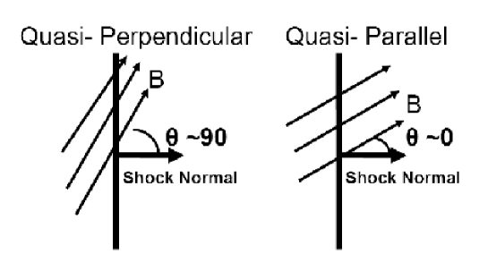
If the angle of the magnetic field to the shock normal is approximately zero degrees the shock is quasi-parallel. This type of shock allows the ions to easily cross the shock as the parallel velocity of the ion is aligned with the bulk fluid flow, v_shock. If the angle of the magnetic field to the normal is approximately 90 degrees, the shock is quasi-perpendicular. Perpendicular shocks inhibit the ion movement with the fluid across the shock front.

Parallel or quasi-parallel shocks are known to heat ions by a two step process (Lee and Wu, 2000). At the shock front, a concentration of ions occurs creating a density ramp. When the ions ”see” this density ramp the ions are scattered by whistler waves and by back streaming ions that were reflected by the higher density material. The backstreaming ions then heat the ions that are near the density ramp as they flow upstream of the shock.

Perpendicular shocks are known to heat ions by processes based on diffusion. All shocks regardless of magnetic angle will dissipate the ram energy of the plasma flow into thermal energy. If the mechanism of dissipation is based on the resistivity and viscosity due to waves excited by some instability due to departure from equilibrium, the shock is considered subcritical. When a shock cannot dissipate its energy by viscosity and resistivity alone, it is classified as supercritical. Ions are heated more than electrons creating a two fluid system which lends itself to many instabilities such as the fire-hose or two-stream instabilities. As the electrons and ions pass into the compressed magnetic field downstream of the shock, their gyroradii are much different setting up an effective potential. This potential decelerates the electrons and reflects a small amount of the protons upstream, which can gyrate gaining energy (Bale et al., 2002). Once the reflected ions are directed downstream through other scattering, this effectively heats the ions that were directly transmitted (Leroy et al., 1982). In a subcritical quasi-perpendicular shock, heating is due to non-deflection of upstream ions at the shock’s ramp (Lee et al., 1986, 1987). As they pass through the shock, the direction of the magnetic field along which they are travelling changes. This causes the ions to start gyrating around the magnetic field increasing their perpendicular velocity by the proton gyro-velocity.

Although for simplicity the shock front is assumed to be planar and laminar, in reality there is turbulence and a physical scale over which the parameters change from the upstream to downstream values. The magnetic structure of the shock affects the density, velocity and temperature. For perpendicular shocks, the magnetic field has a three part structure: a foot, a ramp and then an overshoot of the downstream value for the magnetic field (Baumjohann and Treumann, 1997). The shock foot is a gradual rise in the magnetic field before the shock passes. Next a sharp increase called the ramp occurs. The ramp overshoots the downstream value before coming to an average downstream value. For a laminar flow, these transitions are rather abrupt. However, as there is increasing turbulence and non-linearity to the flow, the magnetic field is characterized by waves and the region of the rise in magnetic field is widened. Parallel shocks have a highly oscillatory pre-shock magnetic field that is called a foreshock region. These transition regions play a key role in heating of ions.

Another measure of the importance of the magnetic field to heating is the relation of the jump conditions with respect to the magnetic pressure. Shocks that have an increasing Alfvenic speed or, in other words, an increasing magnetic pressure are classified as fast shocks. The fast shock bends the magnetic field toward the shock surface and increases the magnetic field. The particles crossing the shock increase their velocity due to the added magnetic field that influences their gyration. If there is a decreasing magnetic pressure across the shock, the shock is classified as a slow shock. The slow shock bends the magnetic field towards the shock normal and decreases the field strength. This thesis focuses on fast shocks because they are most prevelant in the current data set.

Shocks in the heliosphere originate in some way from our Sun. A brief introduction to the Sun and the processes in the solar wind that creates shocks follows.

1.2 The Sun-Our Star

The Sun is an ordinary dwarf variable star of spectral type G2V. It is not the brightest, heaviest, or most unusual star known but is our source of light, heat, energy, and our nearest stellar laboratory. The Sun is a gaseous sphere made up of an interior and an atmosphere each with several layers of varying temperature, density, and dynamics. At a mass of 1.99 x 10³⁰ kg and a radius of 7 x 10⁵ km, the Sun dominates our solar system with 1000 times the mass of the rest of the solar system. The Sun is made up of 74% Hydrogen, 25% Helium, and 1% of other heavy metals by mass (Kaufmann, 1991). The Sun is the greatest accelerator of particles in the solar system. In most cases, it does so by forming shocks in its atmosphere. We shall describe the Sun and its atmosphere as a basis for our shock study involving Coronal Mass Ejections.

1.2.1 Solar Structure

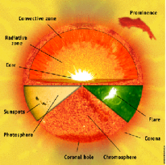
The layer structure of the Sun is shown in Figure 1.3. It consists of an interior and an atmosphere. Three layers make up the interior of the Sun: the core, the radiative zone, and the convective zone. The solar atmosphere is also characterized by of three temperature regimes: the photosphere (cooler=5800 K), the chromosphere (warmer), and the corona, the hottest and part of the atmosphere that is least understood.

Figure 1.3: The structure of the Sun. In addition to the interior structure, coronal phenomena such as flares, holes, and prominences are shown. Adapted from the SOHO website http://sohowww.nascom.nasa.gov

The inner most region of the Sun is the high temperature core. Temperatures in the core reach 15 x 10⁶ K (Carroll and Ostlie, 1996). The core is approximately one quarter of the radius of the Sun yet contains 50% of its mass (Carroll and Ostlie, 1996). At these temperatures and densities, atoms are stripped of all their electrons and protons are readily available for fusion to occur. Nuclear fusion of hydrogen to helium releases energy and neutrinos. The fusion at the core of the Sun creates immense heat which causes the surrounding plasma to expand away from the core. However, gravity counteracts this pressure and maintains the Sun’s structure. The enormous pressure, density, and temperature produced by fusion is a self fuelling process that results in further heating in order to produce heavier fusion products. The Sun is 4.5 billion years old and will continue to convert hydrogen into helium via nuclear reactions for another 5 billion years (Carroll and Ostlie, 1996).

Energy produced by the Sun at its core then travels through the five outer regions in order to reach interplanetary space. Directly above the core is the radiative layer; photons carry energy through this region hence the name. It takes 1 million years for a photon to diffuse through the radiative layers via absorption and re-emission (Kaufmann, 1991). As one moves out in radius from the center of the Sun to the top of the radiative layer, the temperature falls off to 2 $\times$ 10⁶ K.

At the base of the chromosphere temperatures are approximately 4400 K however only 2000 km higher at the top of the chromosphere the temperature rises to 25000 K. Then in the corona the temperature rises from 25000K to 1-2 $\times$ 10⁶ K. One of the many remaining mysteries of the Sun is the heating that occurs in the transition region. This region lies between the cool chromosphere and the extremely hot corona. The rapid rise in temperature indicates an explosive energy source in this region (Moore et al., 1999).

The outermost layer of the atmosphere is the corona. The corona was identified in 968 A.D. by viewing an eclipse (Hetherington, 1996). Further studies in the 1900’s revealed that the corona is a highly dynamic, complex, magnetically dominated region just beyond the chromosphere. From modern studies using coronagraphs, many interesting features have been identified in the corona: flares, prominences, arcades, and coronal mass ejections (CMEs) to name a few. Flares, whose association with CMEs has been hotly debated, are an explosive, rapid release of photons with a frequency range from the X-rays to Radio (Kahler, 1992). Prominences or filaments consist of cool plasma on magnetic loops that extend above the surface of the Sun (van Ballegooijen and Martens, 1989). Coronal mass ejections are a release of large amounts of energetic particles (10¹⁵ grams) (Gombosi, 1999), magnetic energy, and lower energy charged particles into the heliosphere; they will be discussed in the next section.

The number of sunspots, flares, CMEs, and streamers vary with an 11 year cycle. It takes 11 years to progress from minimum solar activity through maximum solar activity and back to minimum conditions. This illustrates how these phenomena are closely tied to the magnetic field of the Sun.

1.2.2 Solar Wind

The Sun has a steady but highly variable supersonic outflow of charged particles, magnetic field, and energy called the solar wind. The solar wind is bimodal, fast or slow, with velocities ranging from 400-900 km sec^-1. At 1 AU, normal densities for the slow wind are 8 cm^-3 (Gombosi, 1999), with a proton temperature of 1$\times$ 10⁵ K and a speed of v 400 km sec^-1. In the fast solar wind the density drops to around 2.5 cm^-3 and with a mean speed of 770 km sec^-1(Gombosi, 1999).

The fast solar wind is associated with coronal holes located near the poles of the Sun during solar minimum. This fast wind is relatively steady as well as relatively uniform in composition. In contrast, the slow solar wind is highly variable and less predictable. The slow solar wind is associated with field lines near closed magnetic regions that open up and allow an outflow of material for a short time (Wang and Sheeley, 1990; Fisk, 2003).

The solar wind varies with the solar cycle. During solar minimum, the fast wind originates mainly over the poles of the Sun but expands in latitude to fill a large region of the heliosphere (Habbal et al., 1997). During solar minimum, the slow solar wind is confined to the equatorial region. During times of elevated solar activity the solar magnetic field becomes highly disordered. Coronal holes occur at all latitudes and are smaller. Therefore, the fast wind is not restricted to the polar area (Woo and Habbal, 1997). Similarly, slow solar wind sources extend to higher latitudes.

The Sun’s magnetic field is carried radially outward by the solar wind. However, the Sun differentially rotates. The Sun’s rate of rotation from its equator to its poles varies but averages 27 days. This rotation twists the magnetic field into a Parker spiral as it is carried away from the Sun in the solar wind.

Figure 1.4: The heliosphere, where the solar wind ions dominate, extends well beyond Earth. This view of the heliosphere shows the planets as well as the meeting of the heliosphere with the interstellar space. From the ACE website http://helios.gsfc.nasa.gov/ace/gallery.html

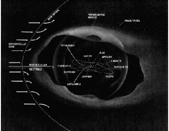
The solar wind does not continue on indefinitely. The heliosphere is the region in space where the Sun s magnetic field and the solar wind dominate, see Figure 1.4. The solar wind stretches well beyond the planets to a point where its pressure eventually equals that of the interstellar medium. A shock is created where the solar wind meets the Interstellar Wind. At this point the solar wind has slowed down and becomes subsonic forming a termination shock. The termination shock is thought to occur between 80 and 100 AU (Belcher et al., 1993). The heliopause marks the boundary between the heliosphere and the Interstellar Medium (ISM). Inside the heliopause, the Sun controls the environment, whereas outside of the heliopause the environment is dominated by the interstellar medium.

1.3 Coronal Mass Ejections

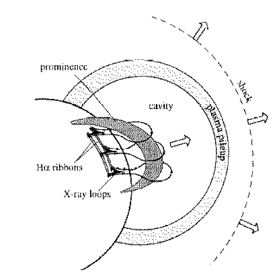
Coronal mass ejections (CME) were first identified in the 1970’s (MacQueen, 1980) using coronagraph images. CMEs are a transient phenomena on the Sun that involve a catastrophic reorganization of the magnetic field and release of mass. Coronal magnetic loops elongate and then pinch off, or reconnect, releasing vast amounts of magnetic field and energy into the heliosphere. The material released in CME, just like the solar wind, includes electrons, protons and heavy ions. The mass released in CMEs is approximately 10¹⁵ grams and carries along the embedded or frozen-in magnetic field as it expands into interplanetary space. The magnetic energy associated with this release is in the range of 10³¹ - 10³² erg (Gosling et al., 1974, 1997). CMEs generally have a three part structure. First is the initial bright dense front or plasma pile-up. Behind the pileup is a dark, low density cavity surrounding the inner most part of the CME, a bright high density core. This structure is illustrated by Figure 1.5 adapted from Forbes (2000).

Figure 1.5: Schematic of the structure of CME as it leaves the corona. A three part structure is present, the plasma pile up, the low-density cavity, and the bright high density core formed by the prominence. Adapted from Forbes (2000)

Once the CME leaves the corona, it expands into the heliosphere with a velocity between 200 km s^-1 to 2000 km s^-1. A CME is seen leaving the corona in the SOHO-LASCO C2 image Figure 1.6.

Figure 1.6: A LASCO C2 image of a CME expanding out of the corona in the top right corner of the picture. Faint loop structures can be seen as the plasma is being expelled from the corona. From sohowww.nascom.nasa.gov

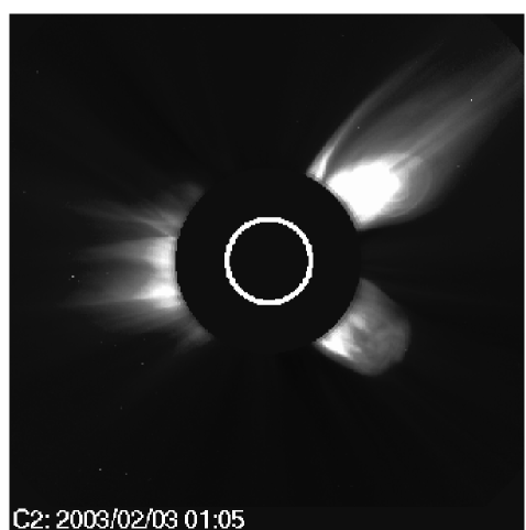
As the CME propagates through the heliosphere it is then termed an Interplanetary CME or ICME. ICMEs are of vast interest in the space weather community as their effects pose a great danger to our satellites and human activity in space. Due to their dynamic interaction with the ambient solar wind, the ICMEs cause shocks to form as they propagate (Stepanova and Kosovichev, 2000). These shocks accelerate high energy particles that pose a threat to astronauts. The collisionless shock ahead of the ICME heats ions and transfers energy into the heliosphere. These shocks are vital to understanding the energetic particles that are detected. This thesis focuses on these shocks as well as other collisionless shocks that are responsible for heating and acceleration of particles such as those associated with supernova remnants.

1.4 Supernovae

The most efficient accelerator in our galaxy and the source of the highest energy particles are supernova. These powerful explosions expel the mass of several suns into the Interstellar Medium and a shock precedes the ejecta.

A star with a mass $\geq$ 1.44 M_⊙, the Chandrasekhar limit (Chandrasekhar, 1984), ends its life in a spectacular explosion: a supernova. Supernovae have been recorded as ‘guest stars’ in the sky by Chinese, Japanese, and Middle Eastern scholars as early as 386 A.D.(Strom, 1994). Their explosions can give off as much light as that of their host galaxies and be hot enough to perform nuclear synthesis during their explosion (Horowitz and Li, 1999).

Supernovae are classified into two types based on the mechanism of their detonation and their emission spectra. Type I supernovae occur when a star runs out of its principle fuel, hydrogen, and a gravitational collapse occurs. The light curve of a Type I supernova has a quick intensity rise to maximum luminosity of more than 10⁹ times the Sun’s luminosity in two weeks. Type I supernovae have a marked absence of hydrogen lines present in their spectra (Charles and Seward, 1995). The dying star is in a constant battle to balance the internal energy produced with the gravity that is trying to collapse the core. The progenitor object, a white dwarf with a companion accreting mass onto its surface, burns hydrogen, then helium, up to carbon and oxygen. When the mass of the white dwarf increases via accretion from its companion to over the 1.44 M_⊙ Chandrasekhar limit, gravity is greater than the electron degeneracy pressure in the stellar core and sends a shock wave inward. The shock wave heats the core so that carbon and oxygen start to fuse. This causes an explosion or deflagration, an explosion without an initial shock wave, that rips apart the star while sustaining enough energy to fuse elements up to radioactive ⁵⁶Ni. The ejecta move outward with an expansion velocity of up to 15000 km s^-1 (Charles and Seward, 1995). There are supernova subtypes such as 1a and 1b that depend on the mass of the progenitor star and brightness of the light curve.

A Type II supernova starts from a more massive star, M$\geq$10 M_⊙, which is a relatively young progenitor that still has its hydrogen envelope, explaining the appearance of broad hydrogen in its spectra. Such a heavy star evolves through a series of burning and contracting that uses increasingly heavier elements for fuel. This gives the star an onion like structure of elements. The last of the fusion products in the interior result in an iron core. There is no energy gain from fusing iron, thus making this an endothermic reaction, requiring external heating to continue. Iron itself cannot fuse, however the silicon in the layer above the core is still fusing into iron increasing the mass of the core and disturbing the delicate balance of electron degeneracy pressure in the core and gravity. The core contracts and iron fissions into lighter nuclei, adjusting the pressure causing gravity to overcome the electron degeneracy and fuse the center of the core into a nuclear density: a neutron star. A neutron star has the mass of the Sun within a radius of 10 km. The light curve of a Type II supernova rises more slowly to maximum and has a lower intensity than a Type I supernova. They are not found in older stellar population but in gas rich young spiral galaxies supporting the hypothesis that these are relatively young stars.

1.4.1 Supernova Remnants

Although the light from the initial explosion of a supernova can be observed for many weeks, and in non-visible light for more than a year, they leave a remnant behind that lasts for 10,000 years. The ejecta expand spherically and supersonically into the local ISM creating a shock around the supernova. There are also two types of remnants: the shell-type remnant and the Crab-like remnant. The shell-type remnant, such as that in the Cygnus Loop or SN1006, blows out the center of the cavity creating a ring of emitting material near the shock wave. The Crab-type remnants, named for the Crab Nebula, have a central source, a neutron star, with jets that fill the interior of the shock cavity. There are four stages of the supernova remnant expansion, regardless of the type of supernovae. The four stages of evolution are free expansion, adiabatic expansion or Sedov-Taylor phase, radiative, and constant momentum phase.

During the free expansion phase (Chevalier, 1982), the shock from the explosion of the star is propagating through the interstellar medium and sweeping up mass. At this phase, the remnant is expanding adiabatically into the ISM. The temperature of the remnant scales as

$$T=R^{-3(\gamma-1)}$$ (1.16)

where $\gamma$ is the ratio of specific heats.

At this phase the kinetic energy of the shock is converted to heating of the swept up ISM material. During this phase, the remnant can be observed in the x-ray and radio wavelengths. The end of this phase is reached when the amount of the material swept up is equal to that of the mass of the ejecta from the supernova. This occurs around 1000 years or $\sim$3 parsecs depending on the density of the interstellar medium and the initial mass of the ejecta.

The second phase, the Sedov-Taylor phase (Sedov, 1959), slows the bulk velocity of the shock because the mass that has been swept up is greater than that of the ejecta. The deceleration of the shock causes a density build up near then leading edge of the shock. The gas in this shell becomes supersonic and a reverse shock is formed between the hot gas of the shell and the inner material of the supernova remnant. This shock heats the outer portion of the supernova remnant recycling the kinetic energy lost in adiabatic expansion back to heat the ejecta. This heating leads to soft X-Ray emission lines that can be used to study the shock characteristics as well as the composition of the ejecta and the interstellar medium. Specifically, the OVI ion is used to trace temperatures greater than 3 $\times$ 10⁵ Kelvin in the far UV ($\lambda$ = 1032,1038 Å).

Due to further expansion, the remnant begins to cool. When it is cooled to around 10⁶K, the material radiates away most of its internal energy and the remnant enters the radiative phase (McKee and Ostriker, 1977). The emission of lines of heavy elements become a key observable at this phase of the supernova remnant. The emission decreases as the remnant expands until it fades into interstellar space or the constant momentum phase. At this time the velocity becomes subsonic and no longer can continue supporting a shock. The constant momentum phase equilibrates the ejecta with the surround interstellar medium spreading heavy elements into the ISM.

1.4.2 Supernova 1006

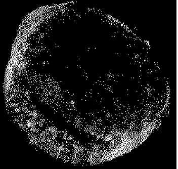
Supernova 1006 (SN1006), with a well known age, distance (Winkler et al., 2003), and shock speed (Ghavamian et al., 2002) was chosen to perform shock studies in this thesis. Located in the southern constellation Lupus, it was first recorded at its brilliant optical peak April 30, 1006 A.D. It was recorded by astronomers in present day China, Iran, Egypt, and Southern Europe. The remnant of SN1006, a Type 1a remnant, is large in the sky, about the size of a full moon. It has been measured to be at a distance of 2.1 kpc (Winkler et al., 2003). With a mean expansion rate of 8700 km s^-1, it is $\sim$18 pc wide (Winkler et al., 2003). This young supernova remnant is entering the Sedov-Taylor phase of supernova remnant evolution.

Figure 1.7: A composite ROSAT HRI image of SN1006 displayed in false color derived from the ROSAT PSPC spectra. Blue represents non-thermal emission, red represents thermal emission. Adapted from Willingale et al. (1996)

SN1006 has been observed at radio (Pye et al., 1981), optical (Ghavamian et al., 2002; Kirshner et al., 1987; Smith et al., 1991), ultraviolet
(Raymond et al., 1995) and X-ray (Winkler et al., 2003; Long et al., 2003; Bamba et al., 2003) wavelengths. Gamma ray observations (Tanimori et al., 1998) were reported but not confirmed. Thin, pure Balmer line filaments were found in the optical observations. In the radio and X-ray, the remnant has a limb-brightened shell structure with cylindrical symmetry around a SE to NW axis probably aligned with the ambient galactic magnetic field (Reynolds and Gilmore, 1986; Jones and Pye, 1988). The NE shock front of SN1006 shows strong non-thermal X-ray and possible gamma ray emission while the NW shock shows very little non-thermal emission at radio or X-ray wavelengths. Figure 1.7 is an image of SN1006 from the ROSAT satellite.

1.5 Instrumentation

Several satellites were used to collect the data for this thesis. The Far Ultraviolet Spectroscopic Explore (FUSE) (Moos et al., 2000) and the Advanced Composition Explorer (ACE) (Stone et al., 1998) were the main satellites, although comparative data was used from Solar and Heliospheric Observatory (SOHO), Cerro Tololo INTER-AMERICAN OBSERVATORY (CTIO) 4-m Ground based Optical Telescope, ROSAT X-ray Telescope, and CHANDRA X-ray Observatory.

The Advanced Composition Explorer (ACE) and the Solar and Heliospheric Observatory (SOHO) take in-situ measurements of the solar wind and the shocks that occur within the solar wind. Observations are made of the atomic emission spectra with the FUSE Satellite to find out physical processes from the shocks that occur outside of the heliosphere allowing for the study of shock parameters of distant astrophysical objects such as SN1006.

1.5.1 Far Ultraviolet Spectroscopic Explorer(FUSE)

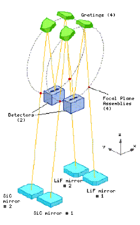
The UV observation of Supernova 1006 was performed with the Far Ultraviolet Spectroscopic Explorer (FUSE) Satellite. The satellite was launched on June 24, 1999. FUSE is in orbit 760 km (475 miles) above the Earth. Its primary objective is to observe in the ultraviolet from 900-1200 Å . The spectrograph is optimized to observe the O VI line in the interstellar medium and in stars. A schematic of the spectrograph design is shown below in Figure 1.8.

The FUSE spectrometer consists of four independent channels with two segments each. When photons enter the instrument they are directed onto one of four different mirrors of the spectrograph. These photons are then reflected onto four different gratings. These gratings then reflect the light into four distinct wavelength regions on two detectors. Four of these eight segments operate in the wavelength range for the O VI doublet, $\lambda$=1031.91, 1037.61 Å. However, the Silicon Carbon (SiC) coated channels, because they are optimized for $\lambda$ $\leq$ 1020 Å, add an unacceptable amount of noise to the faint signal, so only the Lithium Fluoride (LiF) channels are used. These two segments are designated LiF1A and LiF2B. The LiF1A channel covers wavelengths 987.1 - 1082.3 Å, while the LiF2B covers 979.2-1075.0 Å.

Figure 1.8: Schematic of the UV Spectrometer aboard the FUSE Satellite. From the FUSE website fuse.pha.jhu.edu/support/guide/guide.html

Data collected from the detector are processed through the FUSE Pipeline in order to extract the photons per wavelength information that can be analyzed for spectral emission information.

1.5.2 Advanced Composition Explorer (ACE)

The Advanced Composition Explorer satellite (ACE) provided the data used for the Coronal Mass Ejection study. ACE was launched from a Delta II rocket in August 1997. ACE orbits the L1 point, the point where the gravitational forces of the Earth and the Sun are equal to the centripetal force required for the spacecraft to rotate with them, keeping the position between the Sun and Earth constant, about 1.5 million km from Earth and 148.5 million km from the Sun. In its elliptical orbit, ACE can readily view the Sun and the galactic region beyond the Sun.

Of ACE’s suite of nine instruments, three were used in the coronal mass ejection study, the Solar Wind Ion Composition Spectrometer (SWICS), the Solar Wind Electron, Proton, and Alpha Monitor (SWEPAM), and the Magnetometer instrument (MAG).

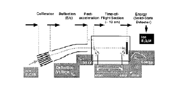
SWICS performs measurements of the chemical and ionic composition of the solar wind (Gloeckler et al., 1998). This instrument uses electrostatic analysis followed by a time-of-flight region and an energy measurement, seen in Figure 1.9, separating all heavy components of the solar wind providing unique identification of up to 40 ions.

Figure 1.9: Schematic of time of flight setup for the SWICS instruments aboard the ACE Satellite. Adapted from Gloeckler et al. (1998)

SWEPAM measures the solar wind plasma electron and ion fluxes (rates of particle flow) as functions of direction and energy (McComas et al., 1998). These data provide detailed knowledge of the solar wind conditions and internal state every minute. SWEPAM provided temperatures, solar wind speed, and proton thermal speeds.

Electron and ion measurements are made with separate sensors. The ion sensor measures particle energies between about 0.26 and 36 KeV, and the electron sensor’s energy range is between 1 and 1350 eV. Both sensors use electrostatic analyzers with fan-shaped fields-of-view. The electrostatic analyzers measure the energy per charge of each particle by bending its flight path through the system. The fields-of-view are swept across all solar wind directions by the spin of the spacecraft. This allows the instrument to measure the mass, based on position on the detector, and energy based on time of flight in the detector.

MAG is a magnetometer that is able to detect the magnitude as well as the direction of the magnetic field (Smith et al., 1998). The basic instrument is a twin triaxial fluxgate magnetometer system. The two identical sensors are on booms that extend past the end of diametrically opposite solar panels. The instrument measures small fluctuations in the magnetic field. It is important to know the magnetic field because the magnetic field direction and strength are crucial to understanding shock geometry and the solar wind flow properties.

1.6 Specific Topics in this Thesis

This thesis examines the heating of particles as they pass through a collisionless shock. Specifically, the heating of heavy ions and neutral particles at the shock front will be examined. Three parameters of the collisionless shocks, Mach number, M_A, the orientation of the magnetic field to the shock normal, $\theta$_Bn, and the plasma $\beta$ have been identified as the important characteristics in heating at a shock front. Using these three parameters and other supplemental data, three different systems are examined to explain the heating and acceleration mechanisms of heavy ions in shocks.

1.6.1 Heavy Ion Heating in Collisionless Shocks

It was found by Berdichevsky et al. (1997) that the heating in shocks is not proportional to mass, as would be found by bulk thermalization of energy, but 1.2-3.0 times mass proportional for oxygen. This differential heating is of importance to understanding the kinetics of the collisionless shock front as well as the acceleration of particles. The heated ion species are also needed as a seed population for acceleration of particles to cosmic ray energies. ACE satellite data provides plasma measurements of the thermal speeds of several species of heavy ions. These ions were shown to be heated preferentially to protons. These results are contrasted with those of supernovae shock studies (Korreck et al., 2004; Raymond et al., 1995). Here heavy ions are heated less than mass proportionally to the protons. SNRs are known to be cosmic ray accelerators. However, the seed population is not well understood and the less than mass proportional heating does not favor a thermal seed population for cosmic ray acceleration. The differences in speed and density of upstream material which can be represented by the plasma $\beta$, all play a role in the heating mechanisms. By studying the parameter space afforded by CMEs and SNR shocks a mechanism for the heating is sought.

1.6.2 Neutrals at Collisionless Shock Fronts

Neutrals at a collisionless shock front could act as a precursor to the shock or as pick up ions. Neutral atoms that can go through the shock upstream from the downstream area can modify the ramp structure of the shock front. Fast neutral atoms from downstream that can avoid being affected by the shock’s magnetic field can flow upstream creating a precursor that would pre-heat the shocked material. The dynamics of the neutrals at the shock front are of great interest in acceleration mechanisms as they could have high energies creating a seed population for cosmic ray acceleration. In Chevalier and Raymond (1978), the authors describe the mechanism for understanding and tracing the neutrals in the shock front. The H$\alpha$ emission line is made up of two components when a significant fraction of neutrals are present. The two components are a broad component made in two steps and a narrow component that is made up of line emission from excited hydrogen atoms. The two steps to create the broad component are as follows: first a downstream proton must charge exchange with a neutral to become a fast neutral. Next, the fast neutral must be excited. When the fast neutral is excited it gives off the H$\alpha$ emission with a shift according to the speed of the particle. Since the excitation is highly dependant on the proton and electron density and energy, the H$\alpha$ intensity ratio is a tracer for the plasma characteristics as well as the neutral fraction.

Several attempts to understand the effect of this sometimes minor population of particles have been modeled by Lim and Raga (1995) and Lim and Raga (1996). Although the simulations did not match the observed broad to narrow H$\alpha$ components, the distribution of neutrals after the simulation was a ring distribution similar to that of a pickup ion distribution. Since a neutral medium is rare in the heliosphere, the neutral modeling is directed at understanding the shocks such as those in SNRs that interact with the neutral ISM material.

1.7 Thesis Overview

1.7.1 Heating of Ions in the Shock of SN1006

In Chapter Two, ultra-violet spectral observations from SN1006 are discussed. The data from the FUSE satellite show strong OVI spectral lines which are an indicator of temperatures in the shock of over 100 million degrees. The non-radiative, thermal collisionless shock of the Northwest region of the supernova remnant and the non-radiative, non-thermal collisionless shocks in the Northeast region of the supernova remnant will be contrasted. A discussion of this specific collisionless shock will follow with respect to the ion heating, neutral fraction of the pre-shock medium and the role of turbulence in the shock front. This section is based on Korreck et al. (2004).

1.7.2 CME shock ion heating

Chapter Three leads to analysis of Coronal Mass Ejections’ collisionless shocks through situ measurements. Using the ACE satellite data from SWICS, MAG, and SWEPAM instruments, over 20 shocks were studied. Shocks were first classified as perpendicular or parallel as this has been shown to be a parameter that greatly changes the heating. The heating of the heavy ions, He⁺², C⁺⁵, C⁺⁶, O⁺⁶, O⁺⁷, Fe⁺¹⁰, were used as a measure of heating versus Mach number and plasma $\beta$. In addition to the analysis of data, the parallel shock work was used to test the theoretical model of the Rankine-Hugoniot conditions for ions in parallel shocks laid out by Burgi (1991).

1.7.3 Neutral Atoms at the Shock Front: A Monte Carlo Model

Chapter Four summarizes the Monte Carlo modelling done in order to understand the neutrals present in collisionless shock fronts. The main objective of the project was to simulate a broad to narrow H-$\alpha$ component intensity ratios that would be affected by the heating by neutrals. The effect of magnetic angle, initial ionization fraction, shock speed, and equilibration between electrons and protons is discussed. Spectra were simulated from the model and compared with observations made by Smith et al. (1991) of other supernova shocks and simulations done by Lim and Raga (1996).

1.7.4 Summary

Chapter Five summarizes the contribution that this work makes to the understanding of the heating processes in collisionless shocks and outlines future work. The work in this thesis is the most comprehensive study of heavy ion heating in shocks. The knowledge gained from this study impacts not only the system of the specific study but also the remote sensing of shocks in the extreme ultraviolet and X-rays wavelengths. The study shows an ideal example of the use of remote and in situ data to study a fundamental physical phenomena.

Chapter II SN1006 Collisionless Shock Fronts

2.1 Introduction

SN1006 (G327.6+14.6) is a nearby Type Ia supernova remnant at a distance of 2.1 kpc (Winkler et al., 2003). With a mean expansion rate of 8700 km s^-1 it is $\sim$18 pc wide (Winkler et al., 2003). The remnant has a high Galactic latitude and modest foreground reddening, E(B-V)=0.11 $\pm$ 0.02 (Schweizer and Middleditch, 1980). This young supernova remnant is entering the Sedov-Taylor phase of supernova remnant evolution. SN1006 has been observed at radio (Pye et al., 1981), optical (Ghavamian et al., 2002; Kirshner et al., 1987; Smith et al., 1991), ultraviolet
(Raymond et al., 1995) and X-ray (Winkler et al., 2003; Long et al., 2003; Bamba et al., 2003) wavelengths. Gamma ray observations (Tanimori et al., 1998) were reported but not confirmed. Thin, pure Balmer line filaments were found in the optical. In the radio and X-ray, the remnant has a limb-brightened shell structure with cylindrical symmetry around a southeast (SE) to northwest (NW) axis probably aligned with the ambient galactic magnetic field (Reynolds and Gilmore, 1986; Jones and Pye, 1988). The NE shock front of SN1006 shows strong non-thermal X-ray and possible gamma ray emission while the NW shock shows very little non-thermal emission at radio or X-ray wavelengths. Ly-$\beta$, He II, C VI, and O VI lines were observed from the faint optical Balmer line filament of the NW shock of the supernova remnant, by the Hopkins Ultraviolet Telescope (HUT), flown during the Astro-2 space shuttle mission. The observed FWHM of the lines were 2230, 2558, 2641 km s^-1, respectively (the O VI line width could not be measured). A kinetic temperature could be calculated from these line widths. The kinetic temperatures of these species are not equal, because the line widths do not scale inversely with the square root of their atomic mass. Instead, the UV observations do suggest that $T_{ion}\sim\frac{m_{ion}}{m_{p}}T_{proton}$ indicating lack of temperature equilibration between species (Ghavamian et al., 2002).

SN1006 provides an opportunity to investigate parameters of non-radiative collisionless shocks faster than 2000 km s^-1. Collisionless shocks appear in many astrophysical phenomena, from coronal mass ejections (CMEs) in the heliosphere to jets in Herbig-Haro objects. When a shock is non-radiative the detection of emission from the shock front is possible, as all of the optical and UV emission of a non-radiative shock comes from a narrow zone directly behind the shock front. Interactions at the collisionless shock front depend upon mechanisms such as plasma waves to transfer heat, kinetic energy and momentum, and it is not well understood how particles of different masses and charges are affected by these processes. The temperature of the species and the degree of temperature equilibration between electrons, protons and other ions are central to the interpretation of X-ray spectra, which effectively measure electron temperature. The energy distribution of a particle species is important to cosmic ray studies as only those particles at a high energy tail of a particle distribution are available for cosmic ray acceleration.

The method of using H$\alpha$ lines to determine collisionless shock parameters was originated by Chevalier & Raymond(1978) and Chevalier, Kirshner, & Raymond (1980). The H$\alpha$ line has a two component profile. The width of the broad component of the H$\alpha$ line is related to the post-shock proton temperature as a result of charge exchange between neutrals and protons, which produces a hot neutral population behind the shock. The narrow component of the H$\alpha$ line is produced when cold ambient neutrals pass through the shock and emit line radiation before being ionized by a proton or electron. The ratio of the broad to narrow flux is sensitive to electron-ion equilibrium and the pre-shock neutral fraction. The FWHM of H$\alpha$ line was measured to be 2290 $\pm$ 80 km s^-1, with models implying the speed of the shock is v${}_{shock}=2890\pm 100$ km s^-1 (Ghavamian et al., 2002). The H$\alpha$ broad to narrow intensity ratio measured to be 0.84 implies an electron temperature much lower than the ion temperature.

This UV observation from the FUSE satellite focused on the shock front in the NW observed by Raymond et al. (1995) and Ghavamian et al. (2002) and on a region in the NE dominated by non-thermal emission. From the spectra, a broad Lyman $\beta$ line ($\lambda$$\sim$1025 Å) and the doublet of O VI ($\lambda$$\sim$1032, 1038 Å) were analyzed for spectral width, intensity, and flux. We use the line widths of the NW and the intensities of the O VI lines in the NE and NW shock fronts to compare the electron-ion and ion-ion temperature equilibration efficiencies as well as densities. The heating of different particle species by the shock front as well as parameters of collisionless shocks that affect particle species heating will be discussed.

2.2 Observations

The Far Ultraviolet Spectroscopic Explorer (FUSE) has a wavelength range of approximately 900-1180 Å. The Large Square Aperture (LWRS), with a field-of-view of 30” x 30”, with a roll angle of 167^o, was chosen for this observation because models predicted that the O VI emission behind the shock would be spread over 35” (Raymond et al., 1995; Laming et al., 1996). The LWRS has a filled-aperture resolution of about 100 km s^-1.

Although the northwest region of the remnant has been observed before in the UV (Raymond et al., 1995), we have much better spectral resolution and a more optimal aperture size to include the entire ionization region given that it may be larger than 19” (Laming et al., 1996). The apertures used for past observations were 19” x 197” (Raymond et al., 1995) in HUT and 2” x 51” CTIO RC Spectrometer
(Winkler et al., 2003; Ghavamian et al., 2002). We positioned the aperture center to be 5”-10” behind the H$\alpha$ filament where the peak formation of O VI occurs. The NE position was chosen based on the edge of the X-ray filament from Long et al.(2003). FUSE observations of the northwest region, centered at $\alpha_{2000}$ =$15^{{h}}$ $2^{{m}}$ $19.17^{{s}}$, $\delta_{2000}$ =-41^o 44’ 50.4”, were obtained on 23 June 2001 and 26 February 2002 with total exposure times of 35,627 s and 6,690 s. Observations of the northeast region, centered at $\alpha_{2000}$=$15^{{h}}$ $4^{{m}}$ $5.0^{{s}}$, $\delta_{2000}$=-41^o 50’ 40.5”, were obtained on 25 June 2001 and 27 February 2002 with exposure times of 42,365 s and 9,666 s. The locations of observations are shown superimposed on an H$\alpha$ image of the remnant taken with the CTIO Schmidt telescope in Figure 2.1 (Winkler et al., 2003).

Figure 2.1: H$\alpha$ image of SN1006 taken by the CTIO Schmidt telescope from Winkler et al. (2003). Closeup images of the observed filaments are shown in the insets. In each case the interior box, drawn to scale, shows the location of the 30” x 30” FUSE LWRS aperture. The NW blowup is from the same H$\alpha$ image while the NE blowup is a 0.3-8 keV Chandra image (Long et al. 2003).

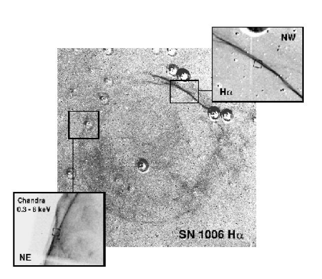
Inserted in the figure is a close up from Chandra (Long et al., 2003) of the NE region of observation to illustrate the x-ray morphology, although no optical emission is obviously present.

There are four components to the background of this observation; detector background, geocoronal lines, the diffuse galactic UV continuum and diffuse galactic O VI emission. The background count distribution on the FUSE detectors is composed of two separate components (Anderson et al., 2003). The ‘intrinsic’ background forms from the $\beta$-decay of potassium in the microchannel plate (MCP) detector glass and the spacecraft radiation environment. The effect of the spacecraft radiation environment on the detector background varies from night to day and with solar activity, but over a short observing time this variation is not significant. The second component is caused by scattered light, primarily geocoronal Ly-$\alpha$. This line produces detector averaged count rates as small as 20$\%$ of the intrinsic background during the night and increasing to 1-3 times the intrinsic rate during the day. The other two components of the background, galactic UV emission and diffuse O VI emission, will be discussed later.

The observations were calibrated with the CalFUSE Pipeline Version 2.2.1. Data from all exposures are processed through the pipeline and then co-added following the FUSE Data Analysis Cookbook and The FUSE Observer’s Guide. The data were selected to contain only the night observations. This greatly reduces the geocoronal background. The night-only exposure times were 32,287 s for the Northwest and 39,386 s for the Northeast.

2.3 Analysis and Results

As mentioned above, the background consists of detector noise, geocoronal lines, diffuse galactic O VI and an astrophysical UV continuum. The first two sources were explained in the previous section, but the additional diffuse UV continuum must be treated separately. It does not originate from SN1006, as it is seen in both of the entirely different regions of the remnant; the NE shock and the NW shock. The diffuse background is attributed to light from hot stars scattering on dust. The diffuse UV continuum is especially bright in this region of the sky according to models by Murthy and Henry (1995). A value of $8.4\times 10^{-15}$ erg cm^-2 s^-1 Å^-1 was quoted by Raymond et al. (1995) while we are seeing approximately $6.5\times 10^{-15}$ erg cm^-2 s^-1 Å^-1 through an aperture one quarter the size of the HUT observation.

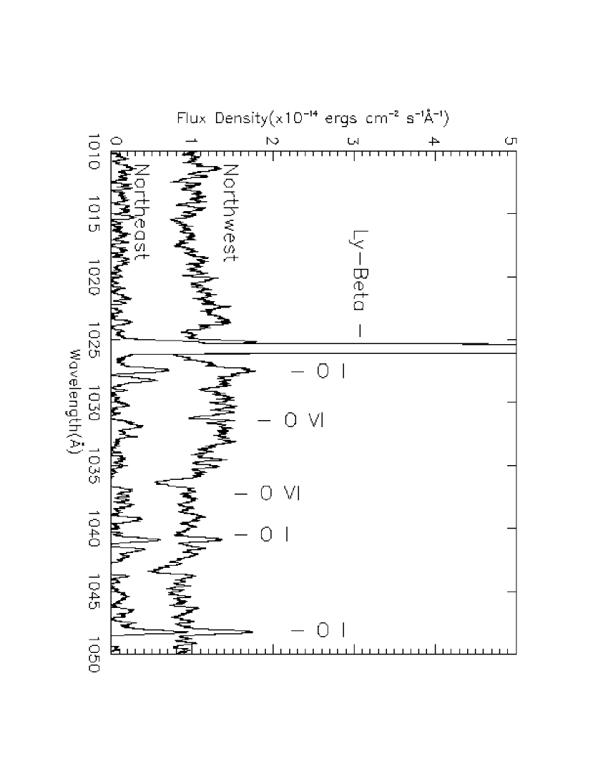
In addition to the diffuse UV continuum, Shelton et al. (2001,2002) and Otte et al. (2003) have found a diffuse O VI background. The brightness of the O VI background is 4700 $\pm$ 2400 photons cm^-2 s^-1 sr^-1 (Otte et al., 2004). The widths of the diffuse O VI lines fall between 10 and 160 km s^-1. In the current NE spectrum diffuse O VI emission has a width of $\leq$ 200 km s^-1 and a brightness of 3500 photon cm^-2 s^-1 sr^-1. We attribute the NE emission to the diffuse galactic O VI background. This enabled us to subtract the NE as a background from the NW data to further eliminate airglow lines, the diffuse UV emission and the galactic O VI background. The intensities of the airglow lines at 1042Å and 1048Å are quite similar in both the NE and NW, further allowing this subtraction. The raw spectra of the NW and the NE regions are shown in Figure 2.2, with airglow lines marked.

Figure 2.2: Raw FUSE spectra from the Northeast and Northwest region of SN1006. The NW is offset from the NE by 0.5 for clarity. Geocoronal lines are marked. The Ly-$\beta$ peak dominates in both spectra. The NE is consistently fainter than the NW, but the geocoronal line intensities are similar.

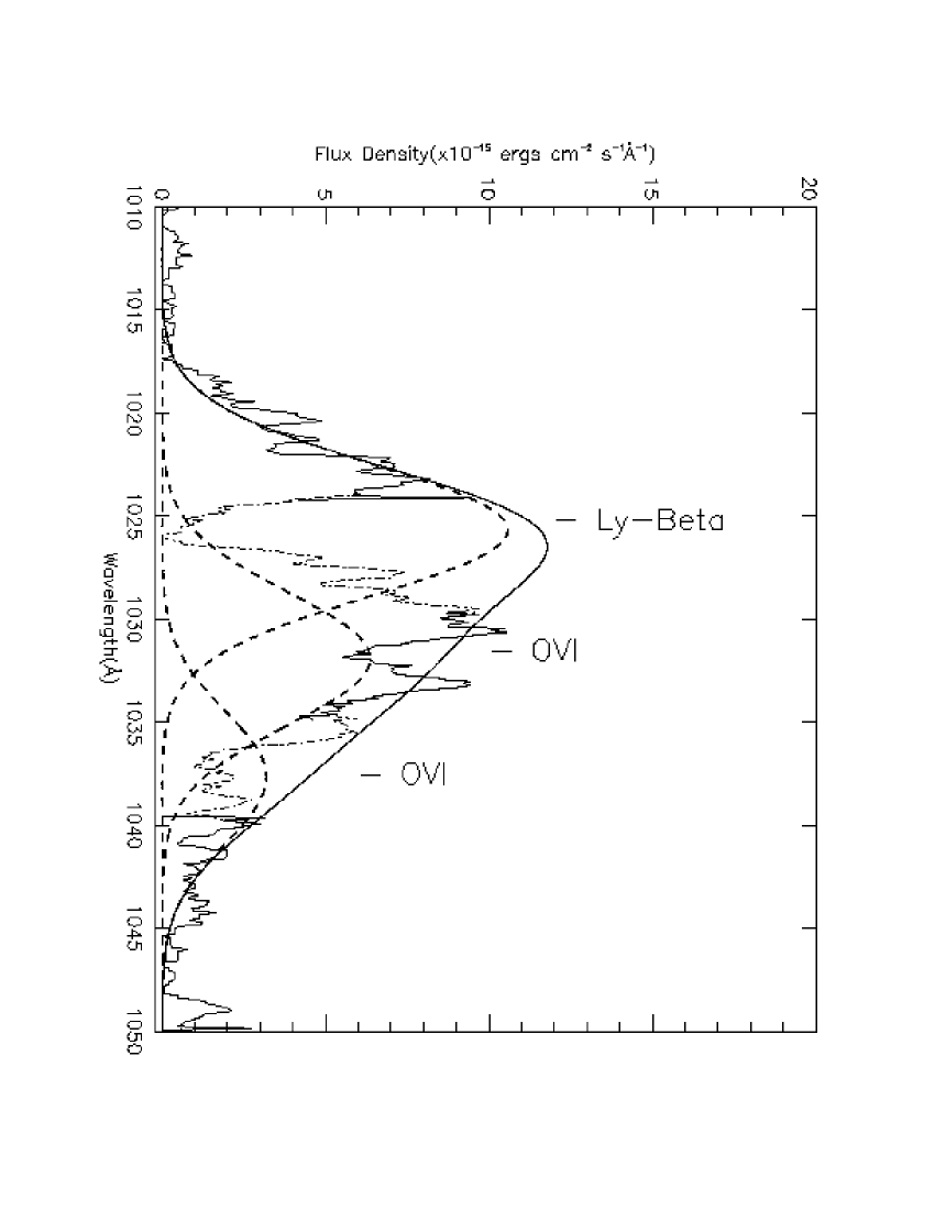
For the NW region, a nonlinear chi-squared minimization routine was used to fit Gaussian line profiles to the spectra. The wavelengths considered for analysis were restricted to 1010-1050 Å to minimize spurious background effects near the ends of the detector’s spectral range. The data were binned by 0.1 Å to increase the number of counts per bin without losing resolution, as the line widths were several Angstroms wide. The width of the broad H$\alpha$ line, from Ghavamian et al. (2002), is v_H=2290 km s^-1. Since the Ly-$\beta$ line is formed by the same process (Chevalier et al., 1980), its line width was set equal to the H$\alpha$ broad component width. The shift of the centroid of the broad and narrow component of H$\alpha$, v=29 km s^-1, is effectively negligible (implying that the shock is viewed completely edge-on) so the broad Ly-$\beta$ line centroid was fixed at its rest wavelength. Only the intensity of the line was a free parameter. The blue wing of the line was fit from 1010 Å to 1024.5 Å. Due to the extinction from interstellar dust, a correction factor must be applied to deredden the observed flux. Using the extinction curves of Cardelli, Clayton, & Mathis (1989), the resulting dereddened Ly-$\beta$ flux is 2.3 $\pm$ 0.3 x 10^-13 erg cm^-2 s^-1.

After subtracting the fitted broad Ly-$\beta$ line profile, the wavelength range from 1022-1028 Å was excluded from the fitting routine in order to avoid negative fluxes and residual airglow that would skew the gaussian fits of the O VI lines. At $\sim$1037.0 Å there were absorption features present that coincided with a C II line and molecular hydrogen lines, along with an O I airglow line. The absorption feature with the spectral range from 1035 - 1038 Å  was therefore excluded from the fit.

The O VI doublet was fit with two gaussians with fixed centers at 1031.91 and 1037.61 Å respectively corresponding to the centroid of H$\alpha$. The doublet line intensities were forced to have a 2:1 ratio but the magnitude of the intensities were allowed to vary. The observed flux is 6.7 $\pm$ 0.1 x 10^-17 erg cm^-2 s^-1 arcsec^-2. Total dereddened flux for the O VI doublet lines was 1.8 $\pm$ 0.2 x 10^-13 erg cm^-2 s^-1. The O VI line widths were measured to be 7.2 $\pm$ 0.4 Å FWHM, or equivalently 2100 $\pm$ 100 km s^-1. The formal error on the fit is 100 km s^-1. However, due to systematic error a more conservative error of $\pm$ 200 km s^-1 is used. The fits are shown in Figure 2.3.

Figure 2.3: FUSE spectra from the NW, binned at 0.1 Å  with the NE subtracted as background. The dotted dashed lines are the regions of the spectra that were excluded from the fits. The dashed lines are the fits for the Ly-$\beta$, O VI 1032 and 1037 Å lines, with FWHM of 2290 and 2100 km s^-1 respectively. The solid line represents the addition of the fits of the three spectral lines.

The width is within the limiting estimate of Raymond et al. (1995) of $\leq$ 3100 km s^-1 and is within 1$\sigma$ error of the H$\alpha$ width of 2290 km s^-1. Although the faint signal in the NE did not allow for a statistically significant fit, an upper limit of O VI intensity was found assuming a width of 2000 km s^-1. The observed upper limit on the O VI line is 1.6 x 10^-17 erg cm^-2 s^-1 arcsecond^-2. An upper limit on the dereddened intensity of O VI in the NE is 4.2 $\times$ 10^-14 erg cm^-2 s^-1. The upper limit of flux for Ly-$\beta$ in the NE is 1.6 x 10^-17 erg cm^-2 s^-1 arcsecond^-2. An upper limit to the dereddened Ly-$\beta$ intensity in the NE region is 4.4 $\times$ 10^-14 erg cm^-2 s^-1.

Past observations of SN1006 line widths and intensities are summarized in Table 1. In order to compare past measurements made with varying aperture sizes, we use intensity per arcsecond measured along the length of the filament. The Ly-$\beta$ from the HUT and the current FUSE observation are consistent. We can use the various measurements to study the ion heating. The proton temperature was found using the shock speed of 2890 km s^-1 from Ghavamian et al. (2002). This proton temperature was then multiplied by m_ion/m_p to calculate the mass proportional temperatures. These calculated temperatures were then compared to the temperatures given by using the FWHM of each ion line. The temperature of O VI as indicated by its FWHM is less than mass proportional by 48%. For the other ions, He II, C IV the heating was also less than mass proportional, by 21% and 18% respectively.

Table 2.1: Summary of UV Emission Lines in NW Filament of SN1006

Ion	Intensity	Filament	FWHM	Temperature	mion/mpT	%
		Length	(km s-1)	(Kelvin)	(Kelvin)	Mass
	(x10${}^{-4})$	(arcsec)	Observed	from FWHM		Prop
H-$\alpha$	2.1	51	2290 $\pm$ 80	(1.8 $\times$ 108 )	-	-
Ly-$\beta$	4.0	30	2290(fixed)
He II	0.99	197	2558$\pm$618	5.7 $\times$ 108	7.2 $\times$ 108	79%
C IV	1.7	197	2641$\pm$ 355	1.8$\times$ 109	2.2$\times$ 109	82%
O VI	3.1	30	2100 $\pm$ 200	1.5$\times$ 109	2.9$\times$ 109	52%
O VII		60	1775$\pm$261	1.1 $\times$ 109	2.9$\times$ 109	38%

The brightness of the O VI lines is proportional to density, n₀, and the depth of the filament along the line of sight. Therefore, an upper limit to the density in the NE can be found by the ratio of intensities provided that the depths along the line of sight are known. Long et al. (2003) calculated a density ratio of n(NW)/n(NE) = 2.5. From the thermal component of the Chandra X-ray spectra Long et al. (2003) estimated a pre-shock ISM density of 0.25 cm^-3 in the NW. Using the limit to the O VI intensity ratio of the NW and NE a ratio of the densities is found to be n(NW)/n(NE) $\geq$ 4, which is within the uncertainties of the Long et al. calculations. Therefore, assuming a pre-shock density in the ISM of 0.25 cm^-3 in the NW, the pre-shock NE density $\leq$ 0.06 cm^-3. This density calculation depends on the assumptions of similar depths along the line of sight in the NE and the NW and of similar numbers of O VI photons per atom passing through the shock. The amount of electron-ion equilibration in the NE would affect these assumptions. Greater electron-ion equilibration in the NE would increase the number of O VI photons per atom (Laming et al., 1996), so the limit on the density in the NE would be even smaller. We attribute the low upper limit on the O VI intensity in the NE to the low density medium into which the remnant is expanding.

2.4 Discussion

O VI lines were not conclusively observed in the faint non-radiative non-thermal NE shock indicating that the two distinct shock regions heat ions differently. Ion heating is important to cosmic ray acceleration and the overall energy distribution of the system. The ions have most of their kinetic energy in a broad distribution which is generally non-Maxwellian as the time to equilibrium via Coulomb collisions for ions and protons is 1.2 $\times$ 10⁵ years (Spitzer, 1956). To understand the heating at the shock front, turbulence, line widths, methods of calculating heating, and the role of neutrals at the shock front will be discussed.

2.4.1 Small Scale Turbulence

Turbulence plays a role in the evolution of fast shocks in supernova remnants (Reynolds, 2004; Ellison and Reynolds, 1991). Small scale turbulence spreads the line profile of an ion much like thermal broadening of a line profile. Since some of the shock energy must be used for bulk flow, we will examine turbulence with a velocity of 1500 km s^-1 which is large enough to affect the spectra but not contain all the energy of the flow. Turbulence decays on a time scale proportional to the characteristic length of the turbulence divided by the velocity of the turbulence $\sim$ $\ell$/v (Tennekes and Lumley, 1972). The width of the H$\alpha$ filament is at most 10¹⁶ cm based on its 1” apparent width on the sky (Ghavamian et al., 2002), making the time scale of the turbulence 10⁸ s $\sim$ 3 years. Using this decay time and the post-shock speed of 750 km s^-1, one quarter of the shock speed, the post-shock region affected by turbulence would be 7.5 $\times$ 10¹⁵ cm. The O VI filament with an observed width of 3 $\times$ 10¹⁷ cm, assuming the 30” FUSE aperture is filled, is also too wide to be dominated by turbulence. Thus the turbulence that is present in the shock of SN1006 is short-lived and not a major source of line broadening.

2.4.2 Line Widths of O VI, UV lines and H$\alpha$

The UV line profiles of the current observations can be compared with past observations of various ion species. The currently observed O VI line width in the NW shock is within 1$\sigma$ of the H$\alpha$ line width previously measured by Ghavamian et al. (2002). Vink et al. (2003) measured an O VII line width of 3.4 $\pm$ 0.5 eV, or approximately 1775 $\pm$ 261 km s^-1 from a different northwest region. This line width is substantially narrower than those of other ion species measured thus far, although the region of observation for this measurement is different from the position of our observations. Along a 124” slit, Smith et al. (1991) found little variation in the H$\alpha$ profiles, indicating that the oxygen temperature does not vary significantly along the length of the NW filament. This implies one of two processes. First, the line width could decline with ionization state and distance behind the shock due to Coulomb collisions, as Coulomb collisions would transfer heat to other species. In Section 2.4.1, we found the Coulomb collision time to be far too long for this process to be important. The second more probable scenario is that some of the lower temperature O VII is from the reverse shock in the supernova ejecta. The detection of Si XIII and Mg XI X-ray lines (Long et al., 2003) in the NW region of the remnant agrees with the hypothesis that the emission is coming from ejecta near the shock front.

The proton temperature quoted thus far used the width of the H$\alpha$ line. However, the proton thermal speed is not simply equal to the velocity derived from the width of the H$\alpha$ line at high temperatures. The cross section for neutral-proton charge transfer, the process that produces the broad H$\alpha$, falls off at high energies allowing for the neutral hydrogen distribution function to be narrower than that of the protons (Chevalier et al., 1980). This results in an H$\alpha$ profile that would incorrectly indicate a lower temperature than the actual proton temperature.

2.4.3 Heating at the Shock Front

Using the current observations the temperatures of the ions are calculated in two ways. The first method to calculate the temperature is based on the thermalization of the bulk velocity of the shock. The second method uses the FWHM of the gaussian line fits as the thermal velocity that can be used to find the temperature. The shock species is heated by bulk thermalization to a kinetic temperature described by the following equation,

$$kT_{i}=\frac{3}{16}m_{i}v_{shock}^{2}$$ (2.1)

where the subscript $i$ indicates the species, $k$ is the Boltzman constant, $T$ is temperature, $m_{i}$ is the mass of the species and $v_{{shock}}$ is the shock speed = 2890 km s^-1 (Ghavamian et al., 2002). This gives a temperature for O VI of 2.9 $\times$ 10⁹ K and for the protons of 1.8 $\times$ 10⁸ K. The ratio of the temperatures is mass proportional, T_oxygen=16T_proton, which is expected using this method. This heating occurs when some fraction of the energy of the shock speed is transferred to the thermal velocity of the protons or ions.

The width of the O VI lines determines the temperature to be 1.5 $\times$ 10⁹ K. The O VI temperature derived from the observed line width is less than that predicted by the kinetic temperature equation for no equilibration among particle species. The ratio of the temperatures indicates that O VI is heated to a temperature 48% less than the value predicted for mass proportional heating. Ions are being heated by a process other than the bulk fluid velocity thermalization or there is a heat loss mechanism for the ions.

Heating of ions in collisionless shocks has been studied by Berdichevsky et al.(1997) using heliospheric shock data. In examining O VII, it was found that the oxygen was preferentially heated 19-39 times more than the protons. In studying the solar wind, Lee & Wu (2000) assume greater than mass-proportional heating as part of the coronal heating process. As a consequence, ions non-adiabatically expand upstream (not being reflected by the shock front) and move with a velocity equal to their gyration velocity as they go upstream. These hot highly energized ions could act as a precursor that takes away a significant amount of energy.

The current supernova observation of less than mass proportional heating lies in stark contrast to the heliospheric collisionless shocks. Several factors and processes determine the extent of ion heating. The first comparison to be made is the speed of the shock relative to the local Alfvénic speed. The solar shocks propagate at 400-1000 km s^-1. SN1006’s shock is propagating at almost 3000 km s^-1. The Alfvénic Mach number, the ratio of the shock speed to the square root average of the thermal and local Alfvénic speed, is $\leq$ 10 for solar shocks but upwards of 200 for the supernova shock. The orientation of the magnetic field with respect to the normal of the shock front is also of importance as quasi-perpendicular shocks and quasi-parallel shocks are quite different. If the current magnetic field orientation for SN1006 is correct, the NW is propagating parallel to the ambient magnetic field, while both parallel and perpendicular shocks are observed in the solar wind.

A measure of the importance of the magnetic field is the parameter $\beta$. The plasma $\beta$, the ratio of thermal to magnetic pressure upstream, is small ($\leq 1$) for heliospheric shocks. Using the parameters for SN1006 and the general value for the Galactic plane ISM magnetic field ($\sim$3 $\mu$G), the NE has $\beta=0.02$ and in the NW $\beta=0.1$. The magnetic field pressure dominates the thermal pressure at the ISM/remnant boundary as in the solar wind, in contrast to the ISM which is assumed to have a $\beta$ of unity. It is possible that the change in density from pre-shock to post-shock conditions is an important characteristic in the propagation and heating of ions in the collisionless shock fronts.

In order to determine the cause of the different heating found in the heliosphere and supernovae further investigation of the influence of pressure, density, Mach number and velocity on ion heating by the shock is necessary.

2.4.4 Neutrals at the Shock Front

In the analysis scheme used here from Chevalier & Raymond(1978) and
Chevalier, Kirshner, & Raymond(1980), neutrals play a vital role. Neutrals undergo charge exchange or emit line radiation to produce the H$\alpha$ and Ly-$\beta$ emission. Shocks produce fast neutrals, as evident by the broad components of the H$\alpha$ and Ly-$\beta$ lines. This could create a neutral precursor for the shock (Smith et al., 1994; Lim and Raga, 1996). The hydrogen and oxygen neutral fractions are tightly coupled by charge transfer, thus information about the neutral fraction of hydrogen can be used to diagnose the neutral fraction of oxygen. These neutrals should become pickup ions like those seen in the solar wind (Vasyliunas and Siscoe, 1976) when they pass through the shock and become ionized. Pickup ions like those in the heliosphere can then act as a high energy seed population for Fermi acceleration just as heliospheric pickup ions are the seed population for anomalous cosmic rays (Fisk et al., 1974).

The He II 4686Å line can be used as an indicator of neutral fraction due to its insensitivity to pre-shock neutral fraction and electron-ion pre-shock temperature equilibrium (Ghavamian et al., 2002). In the NW, observations have shown He II emission lines
(Raymond et al., 1995; Ghavamian et al., 2002). The ratio of HeI/HeII can then be used to find an H neutral fraction which is a parameter in the relation of the H$\alpha$ two component intensity ratio, I_broad/I_narrow, and the electron-ion temperature ratio. In addition, Ghavamian et al. (2002) calculated the pre-shock H population to be 90% ionized but the pre-shock He population is 70% neutral. Using the H$\alpha$ broad-to-narrow intensity ratio calculated for 90% pre-ionized medium, the temperature ratio, T_electron/T_proton, was found to be $\leq$ 0.07, showing little to no equilibration between protons and electrons. Using the ratio of T_electron/T_proton, we find an electron temperature of $\leq$ 1.2 $\times$ 10⁷ K, approximately 1 keV, which is an upper limit that agrees with the value found by Long et al. (2003) of T_electron $\leq$ 0.6 keV, but significantly less than the oxygen and proton temperatures found for this observation(1.5 $\times$ 10⁹ K and 1.8 $\times$ 10⁸ K, respectively).

2.5 Summary

In summary, the two shock regions of SN1006 studied here provide a unique cosmic laboratory for shocks and their acceleration processes. Clearly, the properties of the interstellar medium play a crucial role in shaping these shocks. We conclude with the following summary of our observations and interpretations.

1. The material that the NE shock front is encountering is less dense than in the NW region, with a ratio n(NW)/n(NE)$\geq$4, and is best seen in the X-ray or radio wavelengths. The NW shock front could be moving into a diffuse H I cloud or similarly dense region.

2. The O VI line width of the NW shock indicates that oxygen ions are heated to a temperature less than 48% of the value predicted by mass proportional heating. This differs from the observations of other non-radiative collisionless shock fronts such as those in the heliosphere which found ion temperatures 20-40 times in excess of the values predicted by mass proportional heating. The roles of density, pressure, magnetic field orientation with respect to the shock normal, velocity and Mach number should be examined to better determine the ion heating mechanisms.

3. The plasma at the shock front has not had time to come to equilibrium via Coulomb collisions. The plasma is in a non-equilibrium state with energy distributed differently between species of the plasma. This is in agreement with the work on temperature equilibrium done by Ghavamian et al. (2002) who found the ratio of proton to electron temperature to be $\leq$ 0.07 indicating a plasma far from equilibrium.

The role of the neutral fraction of the ISM population in the charge exchange interaction should be examined in detail as it may greatly affect the outcome of the shock-ISM interaction. The rate at which the plasma becomes isotropic, the particle distribution, and the time scale to reach isotropic and Maxwellian conditions are in need of examination to understand the heating process present in the collisionless shock. Further work will be done to model the plasma conditions in collisionless shock fronts to include neutral fraction as well as examine the role of electron population on O VI formation. This work should help advance the understanding of the shock acceleration of particles and the physics of a collisionless shocks in varying environments.

Chapter III Ion Heating by Collisionless Shocks in Front of Coronal Mass Ejections

3.1 Introduction

The physical properties of the heating mechanism in collisionless shocks and its dependence on the properties of ions are important to understanding the dissipation of energy as a shock evolves as well as the injection of particles into shock acceleration. Coronal Mass Ejections (CMEs) propagating through interplanetary space (IPS) form such collisionless shocks ahead of their ejecta and are ideally suited for this study. CME shocks interact with the solar wind heating and accelerating all solar wind ions. These shocks have been studied both theoretically (Zhao et al., 1991) and through analysis of data from plasma instruments aboard spacecraft in the solar wind (Ogilvie et al., 1980; Zertsalov et al., 1976; Berdichevsky et al., 1997). The heating mechanisms and their dependencies on mass and charge are not well understood. Heating of the plasma can occur in several ways to be discussed later. The most prevalent heating mechanism is bulk thermalization of kinetic energy. However, because there is a magnetic field ever present in the solar wind, interactions of particles via waves and other electromagnetic interactions in the vicinity of the shock must be taken into consideration. The types of waves generated and their effectiveness in heating the plasma vary with particle species and the orientation of the magnetic field to the shock normal (Papadopoulos, 1985).

The data on CMEs from the Advanced Composition Explorer (ACE) satellite afford us the opportunity to study these shocks and their heating processes in greater detail. This study focuses on thermal velocities from the ACE satellite for 21 shocks which are well characterized and for which good data for heavy ions exist. In addition to the proton thermal data, helium, He²⁺, oxygen (O⁶⁺, O⁷⁺), carbon (C⁵⁺, C⁶⁺), and Fe¹⁰⁺ thermal data were available to study. Temperatures of these ions are analyzed in order to study in detail the heating that has occurred in connection with the shock.

3.2 Observations

The ACE SWICS team has been providing data to the ACE Science Center (ASC) since 1998 (Garrard et al., 1998), shortly after ACE launched into its orbit about the L1 point at the end of 1997. The ASC provides the science community with select elemental abundance and ionic charge state measurements . The SWICS instrument (Gloeckler et al., 1998) is composed of an electrostatic analyzer, which measures an ion’s energy per charge, and a time of flight mass spectrometer, which measures an ion’s velocity and total energy. Data obtained from SWICS are analyzed using a numerical code that identifies and characterizes the properties of ions from He to Ni. Triple coincidences (combined start, stop, and solid state detector detection signals) provide identification of the mass (M), charge (Q), and energy (E) of the ions that enter the instrument. However, neighboring peaks overlap due to the resolution limitations of SWICS. The ions are identified and processed in energy-time of flight measurement space using a forward model (Hefti, 1998). The forward model is based on the pulse height analysis (PHA) data accumulated in energy-time of flight matrices. This parameterized model identifies and assigns ions to the appropriate peaks in this measurement space. These peaks or centers are predicted from the residual energy measured in the solid state detector while accounting for the appropriate losses. Due to the limited resolution of the SWICS instrument, some overlap of peaks in measurement space between species may exist. To remove this overlap, gaussian fits are computed for the ion peaks and centered according to the parameterized forward model. Using the gaussian fits, a spillover is calculated and then removed using probabilistic methods, thereby eliminating any statistical biases. The corrected counts are then tallied and assigned to the individual species. The resulting observed distribution functions are then calculated from the ions energy spectra. The distribution functions are then corrected for instrument efficiencies, and sensor duty cycle. From these distribution functions, physical quantities including density, velocity, and thermal speeds can be calculated by taking the 0^th, 1^st, and 2^nd moments respectively.

3.2.1 Error Analysis

The sources for error in the data were both systematic and statistical. The systematic error stems from the measurement technique itself. We assume that all values measured in the instrument are accurate and that statistical counting errors are dominate. Velocity determination was done by taking moments of the phase space density. The accuracy of these moments depends on the counts for the point spread distribution. We use the moments from the gaussian fits to the distribution to get v_th. These real distributions are not always perfectly fit by a gaussian introducing uncertainties. In order to ensure the accuracy of the thermal velocities, the SWICS data were compared to the gaussian fit of the ion distributions for the time period one hour prior and one hour after the shock passage. The detector that is used has velocity resolution or channels that are summed to get the distribution. If the difference between the measured thermal velocity and the fit thermal velocity is less than 3 times the velocity resolution or channel width of the detector, the ion thermal velocity for that shock was considered accurate. Equation 3.1 served as the data filter to indicate the accuracy of the thermal velocities.

$$\frac{2|v_{th}-v_{th,fit}|}{(0.064v_{th})}\leq 3$$ (3.1)

where
v_th is the thermal velocity, v_th,fit is the gaussian fit to the thermal velocity data and the factor of 0.064 is the energy resolution of the SWICS detector. Three channel widths were considered the maximum deviation allowed in order to maintain an accurate measure of the distribution function. The systematic error was then considered as the difference in the fit velocity and the measured peak velocity divided by the measured peak velocity by Equation 3.2.

$$\sigma^{2}=\frac{|v_{th}-v_{th,fit}|}{(v_{th})}$$ (3.2)

Next statistical errors were considered based on the number of counts per ion. The data files available had a density count error. The density being the 0^th moment of the distribution allows for the density counts to be related to the error in the thermal velocity. The average error for He was about 1% whereas the other ions were higher ranging form 1-30%. The statistical error was assumed to be 20% of the value in order to cover the uncertainty in measurements. This statistical error was added to the systematic uncertainty. These errors added together in quadrature were then propagated to find the error on calculated ratios or differences presented in the results and discussion sections.

The other measurements obtained from SWEPAM and MAG such as the proton thermal velocity and the magnitude of the magnetic field were averaged for one-half hour upstream and one-half hour downstream from the time of the shock. This time was chosen to guarantee that the instrument was collecting data on shocked interplanetary medium not the ejecta associated with the CME. There were up to 30 data points available per half hour. Since the website where the date was obtained did not provide errors, we relate the error to the number of data points averaged for our values. The error in this value was then taken to be the inverse of the square root of the number of data points used to compute the mean value.

3.2.2 Shock and Data Selection

A recent article by Cane and Richardson (2003) detailed a list of shocks associated with CMEs from 1996-2002. Cane and Richardson (2003) used low proton temperature and magnetic field rotation data to identify the shock. This shock list was correlated with the shock list kept on the ACE website that details time, magnetic angle, and the Alfvenic Mach number. Observational data from upstream and downstream of the shock were used to calculate plasma parameters using a least-squares fitting of the Rankine-Hugoniot relations. By fitting the observed data the following parameters were available: the shock speed in the spacecraft frame and in the upstream plasma frame in km/s, the angle between upstream magnetic field vector and the shock normal, $\theta_{Bn}$, in degrees, and the upstream Mach number, M_A.

The first criterion for selecting a shock for the study was to have all key data for two hours before and two hours after the shock passage. The next step in data analysis was to determine the structure of the shock based on magnetic angle orientation and the laminar flow of the shock. The temperature of the solar wind provides a measure of the shock and the plasma characteristics upstream and downstream of the shock. An increase in temperature before the time of the shock indicates pre-heating and a possible ramp or reverse shock which needs to be excluded as they heat ions differently. If the temperature increased between the hour and half hour before the shock by more than 30% of the value of the mean of a half hour before the shock, the shock was considered to have a ramp structure and not used in the analysis.

The SWICS, MAG (Smith et al., 1998), and SWEPAM (McComas et al., 1998) instruments that collected the data on ion speed, density, and magnetic field were described in Chapter 1. From the ACE data files, the following parameters were selected:

• Temperature

• Proton thermal velocity

• Proton number density

• He²⁺ ion thermal velocity

• O⁶⁺ ion thermal velocity

• O⁷⁺ion thermal velocity

• C⁵⁺ ion thermal velocity

• C⁶⁺ ion thermal velocity

• Fe¹⁰⁺ ion thermal velocity

• Magnetic Field Magnitude and Direction

The SWICS data have a 12 minute accumulation time. The accumulation cycle that coincides with the time of the shock passage at ACE is not used because the observed data would mix upstream and downstream distributions, exhibiting a two population distribution that would not be able to be fit to a single gaussian.

The proton thermal velocity, the proton number density, and the magnetic field data were taken from the SWEPAM/MAG data set at the ACE Science Center. For the parameters that were taken from the SWEPAM/MAG data set, 64 second averages of data were used. The statistics for these parameters are higher due to the abundance of data for one hour prior and one hour after the shock passage at the ACE satellite.

A plot of representative data for a quasi-parallel and a quasi-perpendicular shock is shown in Figure 3.1 and Figure 3.2. The top panel plots the solar wind velocity as the solid line and the speed of each ion is included as a symbol. The second panel is plot of the number density in the solar wind. The third panel is a plot of the thermal speed of protons with the symbols representing the thermal speed of individual ions. The fourth panel plots the solar wind temperature versus time. The fifth panel contains the magnitude of the magnetic field versus time. The bottom panel is a plot of the magnetic latitude, delta, and longitude, lambda, versus time. In addition, plots of the ion distribution function that were used to determine the thermal velocity, v_th, are included in Figures 3.3-3.6. Each set of plots is labelled with the ion and the charge state. The lower plot of each set is the downstream distribution. The upper panel is the upstream distribution function. Most of the downstream distributions have ”tails” that indicate the distribution is non-gaussian.

Figure 3.1: Plot of ACE magnetic and temperature data versus time, in fraction of a day, for a parallel shock. The top panel plots the solar wind velocity as the solid line and the speed of each ion is included as a symbol. The second panel is plot of the number density in the solar wind. The third panel is a plot of the thermal speed of protons with the symbols representing the thermal speed of individual ions. The fourth panel plots the solar wind temperature versus time. The fifth panel contains the magnitude of the magnetic field versus time. The bottom panel is a plot of the magnetic latitude,delta, and longitude, lambda, versus time.

Figure 3.2: Plot of ACE magnetic and temperature data versus time, in fraction of a day, for a perpendicular shock. The top panel plots the solar wind velocity as the solid line and the speed of each ion is included as a symbol. The second panel is plot of the number density in the solar wind. The third panel is a plot of the thermal speed of protons with the symbols representing the thermal speed of individual ions. The fourth panel plots the solar wind temperature versus time. The fifth panel contains the magnitude of the magnetic field versus time. The bottom panel is a plot of the magnetic latitude,delta, and longitude, lambda, versus time.

Figure 3.3: Plot of ion distributions for a perpendicular shock. Each ion is plotted with downstream data in the bottom panel and upstream data in the top panel. The diamonds indicate the observed data and the solid line is the gaussian fit of that data. Note the drop in magnitude of counts from He²⁺, a major ion in the solar wind, to minor ions such as C⁵⁺.

Figure 3.4: Plot of Iron Distribution for a perpendicular shock. The upstream distribution is plotted in the top panel and the downstream distribution is plotted in the bottom panel. The diamonds represent the observed data and the solid line is the gaussian fit to that data. Note the low distribution versus a major ion such as He²⁺.

Figure 3.5: Plot of ion distributions for a parallel shock. Each ion is plotted with downstream data in the bottom panel and upstream data in the top panel. The diamonds indicate the observed data and the solid line is the gaussian fit of that data. Note the drop in magnitude of counts from He²⁺, a major ion in the solar wind, to minor ions such as C⁵⁺.

Figure 3.6: Plot of Iron Distribution for a parallel shock. The upstream distribution is plotted in the top panel and the downstream distribution is plotted in the bottom panel. The diamonds represent the observed data and the solid line is the gaussian fit to that data. Note the low distribution versus a major ion such as He²⁺.

Figure 3.7: Plot of heating versus Mach number for all shocks. Note that the perpendicular values and the parallel values follow separate trends. The data set is split into perpendicular and parallel data in order to understand the trends in the data.

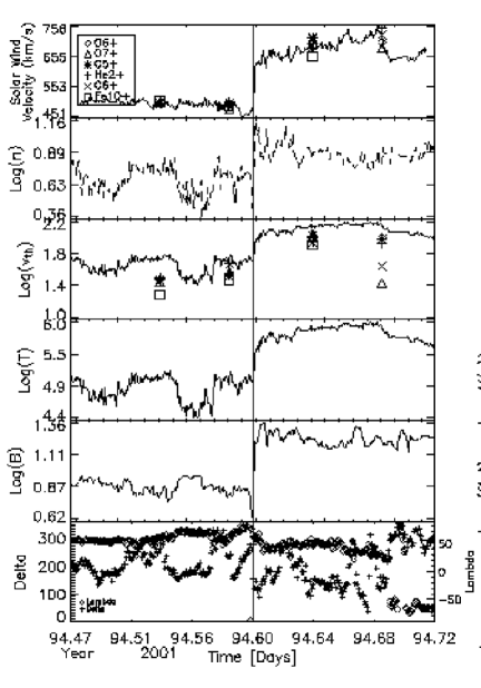
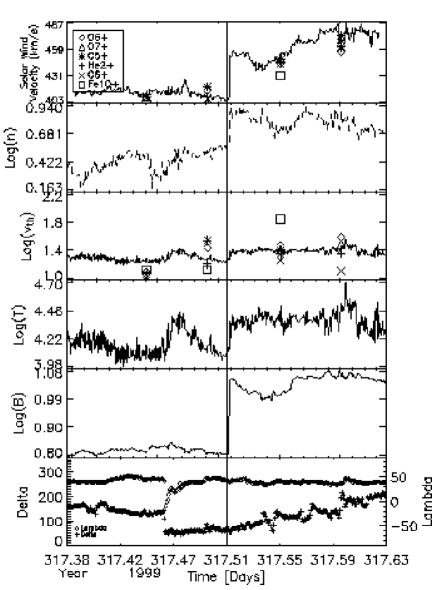
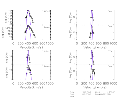
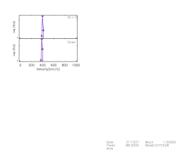
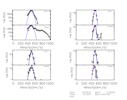
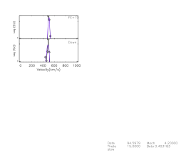
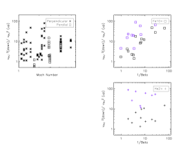
In order to examine the dependence of heating on shock properties most efficiently, the shock list was broken up into quasi-parallel and quasi-perpendicular shocks. It is well known that the orientation of the magnetic field greatly affects the shock characteristics. For example, in Figure 3.7, the magnetic angle is plotted versus Mach number. There seems to be a trend within each of the divisions of parallel and perpendicular shocks but not an overall trend for all the data. Hence, the data set was separated into perpendicular and parallel shocks. There were 16 quasi-perpendicular shocks available for study and 3 quasi-parallel shocks.

From this shock data, calculations of ion heating can be obtained. The heating will be defined as follows for this analysis: the ratio of the change in thermal energy of the species from the upstream to downstream shock region.

$$H=\frac{v_{th_{d}}^{2}}{v_{th_{u}}^{2}}=\frac{3kT_{s,d}/m_{s}}{3kT_{s,u}/m_{s}}$$ (3.3)

where
T_s=Temperature of the species
m_s=mass of the species in units of proton mass
v${}_{th_{d}}$=one hour downstream average thermal velocity of the species
v${}_{th_{u}}$=one hour upstream average thermal velocity of the species
k=Boltzman coefficient

Heating rates are calculated for each ion including protons at each shock event. Heating is summarized in Table 3.1 for perpendicular shocks and in Table 3.2 for parallel shocks. The tables include the Mach number, the magnetic angle, $\theta_{Bn}$, plasma $\beta$ - calculated for upstream protons, and the heating as described by Equation 3.3.

Table 3.1: Summary of Ion Heating in Perpendicular Collisionless Shocks

Year	DOY	Time	MA	$\Theta_{B_{n}}$	Amount of Heating
		UT			p+	He2+	C5+	C6+	O6+	O7+	Fe10+
1999	48	06:20	2.0	100	1.7	0.8	0.8	0.5	0.4	0.2	0.9
1999	63	11:00	2.2	88	1.4	1.1	1.2	1.2	1.0	2.0	4.2
1999	218	06:44	1.5	82	2.4	2.9	9.7	1.7	8.4	4.1	46.9
1999	301	11:30	1.2	83	1.4	0.9	1.2	1.0	1.1	0.7	2.1
1999	317	12:10	1.3	88	1.6	2.5	0.4	4.3	1.1	9.5	27.5
1999	360	09:30	1.1	82	1.3	0.9	0.7	0.7	0.7	0.8	1.4
2001	62	10:41	1.9	82	2.7	2.0	1.0	1.3	1.9	2.1	2.2
2001	98	10:32	4.2	90	4.6	3.1	1.4	4.5	3.4	3.2	3.2
2001	101	15:28	2	98	1.3	0.9	1.4	0.6	1.0	0.8	1.7
2001	118	04:31	5.9	92	10.9	10.6	46.0	0.0	10.2	4.9	12.0
2001	132	09:20	1.2	84	1.0	3.6	2.1	12.0	4.1	0.0	8.9
2001	217	11:55	1.6	88	1.2	0.9	0.4	0.4	0.9	0.7	0.3
2002	107	10:07	2.2	90	1.7	6.5	0.3	5.3	19.0	41.3	17.5
2002	143	10:15	4.2	96	3.6	9.5	8.9	17.9	11.6	9.2	13.1
2002	250	16:10	2.4	89	22.2	14.6	28.3	6.1	78.4	32.0	44.8
2002	313	17:54	2.1	96	1.8	2.3	86.2	0.2	2.5	2.1	1.0

Table 3.2: Summary of Ion Heating in Parallel Collisionless Shocks

Year	DOY	Time	MA	$\Theta_{B_{n}}$	Amount of Heating
		UT			p+	He2+	C5+	C6+	O6+	O7+	Fe10+
2001	23	10:06	2.8	3	5.6	1.9	9.4	14.5	4.8	1.9	7.7
2001	94	14:21	4.2	15	4.5	6.3	4.9	7.0	8.9	9.2	7.5
2001	272	09:07	2.9	19	1.7	1.1	2.0	0.9	1.3	0.5	1.6

Heating of an ion depends on the initial conditions in the upstream plasma. Figure 3.8 is taken from Figure 2 of the Berdichevsky et al. (1997) to compare the results of the current ACE data set with the results of Berdichevsky et al. (1997). The x-axis is the ratio of the thermal speed of He²⁺ upstream to the proton thermal speed upstream. This is a measure of the initial conditions of the plasma. The ratio ($v_{th,i}$/$v_{th,p+}$)_up indicates how close to equilibrium the plasma started. In equilibrium, the ratio of the ion to proton velocity would be proportional to the inverse square root of atomic mass of the ion. Therefore, if v_th,i is less than v_th,p and approximately 1/$\sqrt{m_{ion}}$, the plasma is close to equilibrium. The y-axis is the ratio of the downstream to upstream thermal speed of an ion. The triangles represent the ratio for He²⁺ and the dash indicates the proton. The vertical line connecting two symbols indicates that they are from the same shock. The thermal velocities are the square root of the temperatures of the species. The current data confirms the Berdichevsky et al. (1997) observations where the heating was most prevalent when the initial velocity ratio or x-value was less than 1.0. For ratios of upstream ion to proton velocities greater than 1.0 moderate to no heating occurred.

While Berdichevsky et al. 1997 included helium, oxygen (O⁶⁺), and protons, the current data include O⁷⁺,C⁵⁺,C⁶⁺, and Fe¹⁰⁺ ions extending the mass-to-charge ratio to 5.6. In order to test the mass proportional heating along with the initial conditions of the plasma, Figure 3.9 and 3.10 were created. The x-axis is the same upstream ratio described above for Figure 3.8. The y-axis was constructed as a function of heating. The heating of the ion minus the heating of the proton describes the relative heating of the ions in the shock. As previously stated, the current data confirms a greater heating for x-values less than 1.0. The perpendicular shocks in Figure 3.9 exhibit considerably more heating than that of the parallel shocks in Figure 3.10.

Figure 3.8: Figure 2 from Berdichevsky et al. (1997). The x-axis is the ratio of the thermal speed of He²⁺ upstream to the proton thermal speed upstream. This is a measure of the initial conditions of the plasma. The y-axis is the ratio of the downstream to upstream thermal speed of an ion. The triangles represent the ratio for He²⁺ and the dash indicates the proton. The vertical line connecting two symbols indicates that they are from the same shock.

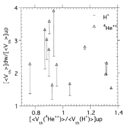
In order to confirm the greater than mass proportional heating, another plot was constructed. The x-axis is the same as that in Figure 3.8, however, the y-axis is adjusted to determine if the heating of the ion is greater than that of the protons. The y-axis is the difference of the increase in the thermal speed of the ion compared to the increase in the proton thermal speed, shown in Figure 3.10 for parallel and Figure 3.9 for quasi-perpendicular shocks. If the difference is greater than zero, the ion is preferentially heated to the protons. Most of the ions lie above this value confirming the greater than mass proportional heating for both types of shocks.

Figure 3.9: Quasi-Perpendicular Shock Heating Ratios versus upstream thermal temperature ratio. The upstream ratio of ion thermal speed to proton thermal speed is the x-axis. The difference in the ratio of temperature increase between the ion and the proton is the y-axis.

Figure 3.10: Quasi-Parallel Shock Heating Ratios versus upstream thermal temperature ratio. The upstream ratio of ion thermal speed to proton thermal speed is the x-axis. The difference in the ratio of temperature increase between the ion and the proton is the y-axis.

Figure 3.11: Heating versus atomic weight. The y-axis is the ratio of temperature of the ion to the proton. The x-axis is the inverse of the atomic weight. The solid line represents the heating expected if the mechanism for heating was mass-proportional. Each ion is averaged for an upstream temperature ratio and a downstream temperature ratio. The larger the atomic mass the more the ion is heated compared to the proton.

Figure 3.12: Atomic Weight versus Heating In Quasi-Parallel Shock. The y-axis is the ratio of temperature of the ion to the proton. The x-axis is the inverse of the atomic weight. The solid line represents the heating expected if the mechanism for heating was mass-proportional. Each ion is averaged for an upstream temperature ratio and a downstream temperature ratio. The larger the atomic mass the more the ion is heated compared to the proton. Note that in the parallel shocks the ratios are much smaller and the differences in values from upstream to downstream, a measure of the temperature increase, is smaller.

To determine the heating according to ion species, Figures 3.11 and 3.12 were created. The x-axis is the inverse of atomic weight. The y-axis is the average amount of heating for upstream and downstream for a particular ion from all perpendicular (Figure 3.11) and parallel (Figure 3.12) shocks studied. The solid line would indicate mass proportional heating. If the species were in thermal equilibrium, the ratio of the square of their thermal velocities would be proportional to 1/$\sqrt{m_{i}}$. The downstream values for four of the six ions are mass proportional or greater as they fall on or above the solid line. However, as atomic weight increases, the heating experienced by the ions increases. This implies a mechanism that is based on weight or mass-to-charge ratio rather than initial temperature. The effect is much greater for the quasi-perpendicular shocks than the quasi-parallel shock. The perpendicular shocks have greater heating ratios than that of the parallel shocks. This seems to indicate that more heating can occur at the perpendicular shocks than the parallel.

Although this and past data sets have confirmed the ions are heated more than the protons in the shock passage, it does not determine the method of heating of the ion species. Next, Mach number and plasma $\beta$ for quasi-parallel and quasi-perpendicular shocks are examined to better determine criteria for the heating mechanism.

3.3 Perpendicular Shocks

3.3.1 Mach Number versus Heating

The Mach number of the shock indicates the shock speed with respect to the Alfven speed in the surrounding material. As the Mach number increases, the critical Mach number is achieved. At this critical Mach number dissipation of energy can no longer be accomplished by viscosity, scalar resistivity or thermal conductivity, other mechanisms such as MHD waves must be invoked.

Figure 3.13: Plot of heating versus Mach number for perpendicular shock. The Mach number is the Alfvenic Mach number. The temperature ratio is the square of the thermal speeds of the ion downstream to upstream.

Figure 3.13, describes the Mach number versus the heating for the perpendicular shocks studied. There is a large amount of scatter in any one ion species. There is no clear trend in heating with respect to Mach number. This is an indication that the bulk thermalization does not play a key role hence the lack of mass proportional heating.

3.3.2 Plasma $\beta$ Effect on Heating

Plasma $\beta$, the measure of thermal to magnetic energy, is plotted versus the heating for each ion species for perpendicular shocks in Figure 3.14. The heating is the ratio of the square of the downstream ion thermal velocity to the square of the upstream ion thermal velocity. $\beta$ is the ratio of thermal to magnetic energies. The plot shows that with increasing $\beta$ the heating of the ions decreases. The mechanism for heating of ions seems to be based on a strong magnetic energy as indicated by a small $\beta$.

Figure 3.14: Plot of $\beta$ versus heating for all the ions in perpendicular shocks. The heating is the ratio of the square of the downstream ion thermal velocity to the square of the upstream ion thermal velocity. $\beta$ is the ratio of thermal to magnetic energies.

Figure 3.15: Plot of $\beta$ versus heating for Fe¹⁰⁺ ions in perpendicular shocks. The heating is the ratio of the square of the downstream ion thermal velocity to the square of the upstream ion thermal velocity. $\beta$ is the ratio of thermal to magnetic energies. Fe¹⁰⁺ shows a clear downward trend in heating with increasing $\beta$.

To further illustrate this heating trend, Fe¹⁰⁺, the heaviest ion investigated as well as the one with the highest mass to charge ratio, was plotted versus $\beta$ in Figure 3.15. The iron heating decreases with increasing $\beta$ as it does for the other ions plotted in Figure 3.14. However, Fe¹⁰⁺ shows the most heating of any of the ions studied. In order to determine if this heating is linked to the mass or the mass-to-charge ratio, two other plots were made. The first, Figure 3.16, plots the O⁶⁺ and O⁷⁺ ion heating. If the dependence on $\beta$ was related to mass only, then these points should be relatively the same. The second plot, Figure 3.17, graphs the heating of the heaviest ion studied, iron and the lightest, helium.

Figure 3.16: Plot of $\beta$ versus heating for Oxygen ions in perpendicular shocks. The heating is the ratio of the square of the downstream ion thermal velocity to the square of the upstream ion thermal velocity. $\beta$ is the ratio of thermal to magnetic energies. If the heating was based on mass these two ions should have identical heating. However, the heating is widely variable for the two ions.

Figure 3.17: Plot of $\beta$ versus heating for Fe¹⁰⁺ and He²⁺ ions in perpendicular shocks. The heating is the ratio of the square of the downstream ion thermal velocity to the square of the upstream ion thermal velocity. $\beta$ is the ratio of thermal to magnetic energies. Although both show a decrease in heating with increasing $\beta$, the Fe¹⁰⁺ ions exhibit more heating than the He²⁺ ions.

The oxygen plot, Figure 3.16, shows variation between the two species. This seems to imply that the mass-to-charge ratio is of importance more than the atomic mass. There are shock events where O⁶⁺ is heated more than O⁷⁺ and vice versa. There is always a separation in the amount of heating. The second figure, Figure 3.17, plots the $\beta$ of helium and iron that shows the mass is indeed not the only factor as the helium does seem to have similar heating. One point to consider is that helium is a major species in the solar wind whereas iron is a minor species. The major species would correlate well with the bulk characteristics of the plasma and a minor ion could not be affected in the same way as it could act as a separate fluid.

3.4 Parallel Shocks

3.4.1 Mach Number versus Heating

Figure 3.18, describes the Mach number versus the heating for quasi-parallel shocks. The heating is that which is described by Equation 3.3. The Mach number is the Alfvenic Mach number. The temperature ratio is the square of the thermal speeds of the ion downstream to upstream. In quasi-parallel shocks, as the Mach number increases, the temperature increase for the ions. However, with the small number of data points it is difficult to define a trend. More parallel shocks would be necessary to fit a trend to the data.

Figure 3.18: Heating versus Mach Number for Quasi-Parallel Shocks. The Mach number is the Alfvenic Mach number. The temperature ratio is the square of the thermal speeds of the ion downstream to upstream.

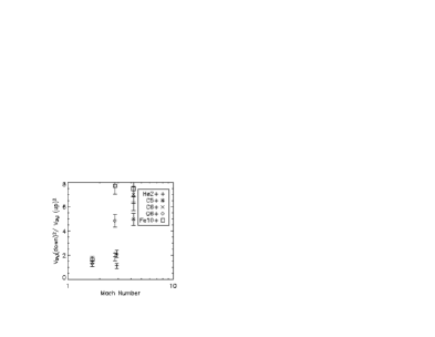
3.4.2 Plasma $\beta$ Effect on Heating

The plasma $\beta$ was also examined for the parallel shocks. The heating versus plasma $\beta$ was plotted for the parallel shocks in Figure 3.19. The heating is the ratio of the square of the downstream ion thermal velocity to the square of the upstream ion thermal velocity. $\beta$ is the ratio of thermal to magnetic energies. There was a shock with higher $\beta$ than that of the quasi-perpendicular shocks. There seems to be a decrease in heating with increasing $\beta$, however with only a few shocks to study the trend is unclear. The Helium has a downward trend where as the Carbon ions exhibited an increase in heating with increasing plasma $\beta$. The lack of statistics makes trend fitting unrealistic.

Figure 3.19: Heating versus Plasma $\beta$ for Quasi-Parallel Shocks. The heating is the ratio of the square of the downstream ion thermal velocity to the square of the upstream ion thermal velocity. $\beta$ is the ratio of thermal to magnetic energies. Due to the lack of statistics there is no clear trend of heating with respect to plasma $\beta$.

3.4.3 Rankine Hugoniot Conditions for Ions

In a paper by Burgi (1991), the Rankine Hugoniot conditions were rederived for parallel shocks with an assumption that the plasma was a multi-fluid plasma. The assumption that the ions and the electrons and neutrals were in equilibrium was relaxed allowing for each charged species to be a separate fluid. For each species, heat flux carried by the ions were neglected because it was small compared to the kinetic energy and enthalpy fluxes. Using conservation equations for continuity, momentum, and energy, the following conditions were found for a specific ion species:

$$[n_{i}u_{i}]=0$$ (3.4)

$$[u_{i}^{2}T_{i,||}]=0$$ (3.5)

$$[\frac{1}{2}m_{i}u_{i}^{2}+\frac{3}{2}kT_{i,||}]=0$$ (3.6)

Equation 3.4 is the continuity equation for each individual species. Equation 3.5 describes the dependence of the momentum on the parallel temperature. The energy equation, Equation 3.6, uses the kinetic energy of the species as well as the thermal energy in the parallel direction as the two sources of energy of the fluid. The quantity in Equation 3.6 will be referred to as $\rho$ in future plots. The data from the parallel shocks in this study were then fit to the rederived conditions. Below in Figure 3.20, plots of the data versus the multi-fluid Rankine Hugoniot conditions are shown. For the multi-fluid approach to be correct, the downstream and upstream values should be equal, represented by the line x=y in the three plots.

Figure 3.20: Fit of CME Shock Data to the Rankine Hugoniot conditions derived by Burgi 1991. One parallel shock is used. The speed is the difference between the thermal speed and the shock speed. Each symbol represents the ratio for a single ion in the shock. The top plot is the continuity equation. The second is momentum conservation. The third plot is conservation of energy. Rho is defined in Equation 3.5.

The mass conservation for the parallel shock is within the errors of the predicted values as well as that for the momentum conservation. However, the energy increase observed is greater than that predicted for these ions. The increase over equality measures the potential across the shock. The acceleration and heating effect of this potential will be discussed in the following section. The data matches the hypothesis of a multi-fluid plasma treating each ion species separately and relaxing the condition of equilibration between the protons, electrons, and ions.

3.5 Discussion of Heating Mechanisms

Bulk thermalization leading to mass proportional heating has been ruled out as the lone source of heating at the collisionless shocks front. Lee and Wu (2000) discuss three parameters key to understanding heating in collisionless shocks: Alfvenic Mach number, magnetic shock angle, and plasma $\beta$. Each dependence has been examined in the coronal mass ejections shocks. In addition to these three parameters there are two other factors to consider, the mass-to-charge ratio and the turbulence around the shock. Also, the thermal state of the plasma ahead of the shock is important to understand heating. The mass-to-charge ratio is important to MHD interactions because of lower-hybrid waves that heat electrons in the shock front (Laming, 2004). In addition to the mass-to-charge ratio, turbulence plays a role in the plasma heating. According to Leroy et al. (1982), supercritical quasi-perpendicular shock heating is largely due to reflected ions at the shock front that cause turbulence. This turbulence then energizes the ions that encounter the shock front. Although the turbulence is likely present at the shock front, the data filtering process took out shock fronts with detectable ramps that would be an indication of turbulent processes.

The interest in heating of the thermal population stems from the cosmic ray acceleration processes. The acceleration mechanisms such as First and Second Order Fermi acceleration require a ”seed population” that is energetic enough to enter into the acceleration process and produce high energy cosmic rays. Second Order Fermi Acceleration was first discussed by Fermi in 1949. The acceleration occurs when particles collide with magnetic eddies or inhomogeneities. The inhomogeneities are moving with a velocity, v. There is different likely hood of a head-on collision increasing the energy of the particle compared to that of a tail collisions decreasing the energy of the particle. The Fermi mechanism goes as the power of v_sc/v_part, where v_sc is the speed of the scattering centers and v_part is the particle speed. Fermi was looking at relativistic particles. The average increase in energy is second order in v/c where c is the speed of light. However, this implies that a velocity has to be fairly large initially (greater than 1000 km s^-1) to effectively heat the ion. The speed has to be great enough that acceleration by scattering happens faster than energy loss by Coulomb collisions, which become less effective as v^-3 First Order Fermi Acceleration is based on a system where the particle increases energy at each scattering center such as a supernova shock where there is scattering centers on both side of the shock front. Each time the particle collides on either side of the shock there is a head-on collision gaining energy. This process is more efficient than the second order Fermi Acceleration with an average energy increase of the order v/c . However the initial velocities in the data set are small compared to c. This mechanism is based on initial energy and does not have any clear relationship to the mass or mass-to-charge ratio heating that is observed in the current shock study.

Looking for a mechanism that can take a thermal particle to a suprathermal particle is necessary for these acceleration processes. From studies of the earth’s bow shock by Fuselier and Schmidt (1997), a heating method is proposed. This heating mechanism is based on the potential that forms around the shock front. Protons are the species that creates the shock. The model assumes the ion is a test particle and that all the velocity change is in the direction parallel to the shock normal. This assumption tells us that the minor ions do not actually form the shock but just experience its effects. The effective electrostatic potential that is set up is created by the change in the proton flow velocity across the shock.

In the shock crossing, a potential is formed, e$\phi$. This potential slows down the proton as energy must be conserved. The potential that was formed by the protons is proportional to the difference in kinetic energy for the proton in transition from upstream to downstream. Therefore, the downstream thermal speed of the proton is proportional to initial velocity minus any slowing from the electrostatic potential.

The heavy ions at the shock front also see a potential. However, they see a potential based on their mass to charge ratio. To conserve energy, the ion speed increases across the shock. The ion’s downstream speed is as follows in Equation 3.7 from Fuselier and Schmidt (1997) :

$$v_{down,i}=v_{sw}\sqrt{\frac{(\alpha-1)+c^{2}}{\alpha}}$$ (3.7)

where $\alpha$ is the mass to charge ratio, v_sw is the solar wind speed which is assumed to be equivalent to the upstream proton speed, and c is the ratio of downstream proton speed to upstream proton speed. This equation for the downstream ion velocity clearly includes a factor of mass-to charge. After the ion passes downstream, it can also be scattered. If this scattering is strong enough to push the ion upstream, an acceleration process can begin. Chapter 4 discusses neutrals and finds that several percent of them overtake the shock. This is a small percent compared to observed cosmic ray flux.

Fuselier and Schmidt (1997) discuss pitch angle scattering and therefore velocity vectors not thermal speeds. In order to relate these velocities to thermal speeds, a simplifying assumption must be made. The average speed of the particle is the thermal speed over the square root of 2 (Baumjohann and Treumann, 1997). In addition, the solar wind speed was assumed to be the same as the ion speed for the upstream conditions. This is unrealistic as most of the speeds measured vary. Squaring the downstream thermal velocity, comparing it with the upstream velocity squared and rewriting the equation in terms of Mach number, Equation 3.7 becomes:

$$\frac{v_{down,i}^{2}}{v_{up,i}^{2}}=\frac{M_{A}^{2}v_{A}^{2}(\alpha-1)+c^{2}}{v_{up,i}^{2}\alpha}$$ (3.8)

Substituting plasma beta in terms of the Alfven speed the heating becomes:

$$\frac{v_{down,i}^{2}}{v_{up,i}^{2}}=\frac{M_{A}^{2}2kT/m_{p}\beta(\alpha-1)+c^{2}}{v_{up,i}^{2}\alpha}$$ (3.9)

There is an inverse dependence on plasma $\beta$ which is similar to what was found in the analysis of the CME data. To further test the relationship, the predicted heating versus plasma $\beta$ was plotted in Figures 3.21 and 3.22.

Figure 3.21: Plotting of the actual and predicted values for heating based on plasma $\beta$. Helium shows similar trends to the prediction but the actual values are higher than those observed.

Figure 3.22: Plotting of the actual and predicted values for heating based on plasma $\beta$. Iron shows similar trends to the prediction but the actual values are higher than those observed.

These figures show similar trends in the heating for both the observational and the predicted values. However, the absolute numerical value is higher for the predictions. The uncertainty in the measurements and of the calculated Mach number could account for this difference. A general dependence on heating of the inverse of plasma $\beta$ coincides with the trends in the observational data.

This accounts for the increase in heating due to the mass per charge ratio of the ion. However, in perpendicular shocks, there could be an additional or alternative heating mechanism. The above model assumed that there are no tangential forces acting on the ions. The ions however are gyrating around the magnetic field with a velocity v_gyro. Again if we assume the relationship between the speed and the thermal velocity, we can see that this gyration will add heating to the ions in the perpendicular case. The perpendicular orientation of the magnetic field to the shock normal means that the ions are gyrating in the x-z plane. Most of the velocity from the gyration is in the x-direction which increases the thermal velocity. This gyrating particle sees the potential and increases the particle’s thermal velocity with the gyration velocity. In a parallel shock the gyration is in the y-z plane and therefore most of the velocity is tangential to the potential and does not affect the heating.

This accounts for the differences in heating as seen between the parallel and perpendicular shocks. The other dependence highlighted by the current data set is the affects of plasma $\beta$ on heating. It is not obvious how this affects the heating.

3.6 Conclusions

This study included an unprecedented data set of different ion species to investigate the heating that occurs at a collisionless shock front. Based on magnetic angle to the shock normal, each set of shocks was analyzed for their dependence on Mach number and plasma $\beta$. In a quasi-perpendicular shock, increasing $\beta$ decreases the heating highlighting the importance of the magnetic field to the heating process. Mach number has little to no correlation with ion heating. In a quasi-parallel shock, increasing $\beta$ again decreases heating. Mach number however does seem to enter into heating at the parallel shocks either.

An acceleration method based on a potential post-shock described by Fuselier and Schmidt (1997) may account for the heating observed in this study. The model explains the heating that occurs at a quasi-perpendicular shock but does not seem to match well with a parallel shock. The parallel shock heating is closer to mass proportional because it is not as affected by the potential as the ions in the perpendicular shock.

There is also currently similar ion heating data available for collisionless shocks in supernova remnants showing non-preferential heating to ions. This begs the question of the ubiquitous nature of the shock physics: what is the dominant factor to determine effect heating at a collisionless shock front? The supernova has a Mach number 10 times that of the CME shocks however, as seen in this data set, the Mach number does not seem to play a major role in determining heating. Density and magnetic energy seem to be of greater importance. Although not examined in this study, a shock precursor can be an addition source of plasma heating. Preheating or a precursor would explain the high heating seen at some of these shock fronts. The next chapter explores neutrals as a source of a precursor and for their role in heating.

Chapter IV The Effects of Neutrals at Collisionless Shock Fronts

4.1 Introduction

Heating at a collisionless shock front was diagnosed by in situ measurements of CMEs and by UV spectral data in SN1006. The thermal speed of pre-shock and post-shock heavy ions in CMEs were compared to describe heating. The spectral line width describes the thermal broadening of the H$\alpha$ and OVI lines in SN1006. The ISM around a supernova is thought to be highly ionized from the UV flash that occurs when the supernova detonates. However, through H$\alpha$ observations and subsequent modeling Ghavamian et al. (2002) concluded that the photons from the UV flash from the initial supernova explosion were not enough to pre-ionize the ISM to the current shock position. Therefore, the SN1006 shock is interacting with a partially neutral medium. The bow shock of the heliosphere also propagates into a semi-neutral ISM. As a fast shock propagates, neutrals will be quickly ionized in the hot plasma downstream of the shock. However, some of the neutrals will be excited and emit H$\alpha$ radiation before being ionized. This emission represents the pre-shock conditions before the physical signatures of the collisionless shock are masked by Coulomb collisions.

Neutrals at a collisionless shock front are therefore important to understand as a diagnostic for the pre-shock conditions as well as the interpretation of the observed spectral lines. In addition, neutrals, because they are not tied to the magnetic fields can run upstream preheating the upstream plasma. This can create a precursor. The study of neutrals is based on the method for diagnosing the degree of ion-electron thermal equilibrium of a shock front using the broad to narrow component intensity ratio of the H$\alpha$ spectral lines (Chevalier and Raymond, 1978). The interactions that produce the two components, narrow and broad, of H$\alpha$ emission are sensitive to neutral fraction. These two components are seen in Figure 4.1 taken from Hester et al. (1994) observations of the Cygnus Loop supernova remnant.

Figure 4.1: The plot, taken from Hester et al. (1994), plots the change is velocity (which indicates change in wavelength) versus intensity. The observed data are ploted as crosses. The fit to this spectral line has two components shown as the solid line without symbols-the broad component and the narrow component.

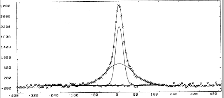
There are two types of neutrals and two types of protons at the shock front, fast and slow. Both types of neutrals and protons are needed to obtain the broad and narrow component of the H$\alpha$ line. Fast protons are those that initially start downstream of the shock. Fast neutrals are fast protons that have undergone charge exchange to become neutral. Slow protons and slow neutrals are from the upstream population. The narrow line is produced when a slow neutral is excited by an electron or a proton. The broad component is formed in a two step process. First, a fast proton must charge exchange to create a fast neutral. The fast neutral must then be excited to emit the H$\alpha$ broad component.

The theoretical ratio of intensities of the broad to narrow components can be calculated by considering the three processes involved in the creation of these components: charge transfer, ionization, and excitation. Chevalier et al. (1980) derived the following relation:

$$\frac{I_{b}}{I_{n}}=\frac{(\sigma_{x}v)_{s}}{(\sigma_{i}v)_{f}}[\frac{\epsilon_{A}}{\epsilon_{B}}+\frac{g_{\alpha}}{\epsilon_{B}}(1+\frac{(\sigma_{x}v)_{f}}{(\sigma_{i}v)_{f}})]$$ (4.1)

where
$\epsilon$=efficiency of H$\alpha$ emission
case A: optically thin medium for the broad component
case B: optically thick medium for the narrow component
($\epsilon$ ranges from 0.1-0.8)
$\frac{(\sigma_{x}v)_{f}}{(\sigma_{i}v)_{f}}$=the probability a fast neutral will undergo charge transfer
g_α=the fraction of emission in H$\alpha$ from charge transfer into an excited state
$\frac{(\sigma_{x}v)_{s}}{(\sigma_{i}v)_{f}}$=ratio of charge transfer to ionization rates.

Fast neutrals created downstream of the shock can migrate upstream of the shock, preheating the unshocked material. There are two steps in computing the pre-shock heating. First, one must compute how much energy is carried upstream by these fast neutrals. Second, the fraction of energy that can be deposited upstream before the particle is swept back through the shock to the downstream side must be calculated.

A fast neutral precursor can contaminate the narrow component of the H$\alpha$ line. An upstream fast neutral can undergo charge transfer or ionization and then excite a narrow neutral component. The number of fast neutrals that can come upstream is still an open question that this study examines. In addition to affecting the intensity profile of the two H$\alpha$ components, neutrals upstream of the shock can modify the jump conditions of the shock by travelling from the downstream region to the upstream region changing the energy, mass, and momentum distribution, physically broadening the transition region around the discontinuity of the shock. This causes a ramp-like structure to form at the shock front. The orientation of the magnetic field also affects the ease of transport of an ion upstream or downstream. The length scale involved in heating the upstream plasma is of importance to understand how much time the shock interacts with the plasma and at what rate energy is transferred.

The plasma at the shock front in the ISM is essentially a three species fluid made up of an electron, proton and neutral components. Each of the three components has a different effect on the shock and is affected differently by the passage of the shock. The charged fluids are affected by the magnetic field whereas the neutral fluid evolves unconstrained by the magnetic field. Multifluid flows have been studied numerically by Draine (1980) and Flower et al. (1985). Chevalier & Raymond (1978) and Chevalier, Kirshner & Raymond (1980), studied the neutral fluid of shocks in supernova remnants through observations of the broad component line width and the ratio of intensities of the H$\alpha$ broad and narrow component. Lim & Raga (1994) simulated the effect of high pre-shock ionization fraction on strong shocks. However, magnetic effects, velocity perpendicular to the flow, and the atomic processes at high energies were not simulated.

In this chapter, a 2-D Monte Carlo particle simulation follows the neutrals as they pass through the shock front. The pre-shock ionization fraction is varied to characterize the effect of the presence of neutrals at the shock front. This simulation results in H$\alpha$ broad to narrow intensity ratios with varying shock speed, magnetic angle, and pre-shock ionization fraction.

4.2 Model Description

A 2-D MHD particle Monte Carlo model was created to follow a neutral particle as it moves through the shock front and interacts with the surrounding plasma. The simulation space was chosen to be four times the ionization mean free path for a hydrogen atom ($\lambda$_mfp $\sim$ 1 x 10¹⁶ cm) assuming a density of 1 particle per cm³. These dimensions ensure that the shock front related emission is all within the computational grid and that any relevant physical interactions would occur within the calculation space. We followed 1 $\times$ 10⁵ neutral particles in order to get statistically significant results.

The density was assumed to be one. The mean free path distance scales are then proportional to $\frac{1}{n}$. The intensities scale as n so that the broad to narrow intensity ratio is independent of n. The simulation is done in the frame of reference where the shock is at rest. Therefore the upstream plasma is moving towards the shock at the velocity of the shock, v_s, and the downstream plasma is moving away from the shock at a quarter of the velocity of the shock, 1/4 v_s. The pre-shock (upstream) plasma is assumed to be in local thermodynamic equilibration; the protons, electrons, and neutrals are in thermal contact and therefore a single fluid. The neutral fluid is assumed to be in a pre-shock Maxwell-Boltzman distribution. The post-shock (downstream) characteristics such as density and temperature are calculated from the Rankine-Hugoniot conservation conditions across the shock, assuming a strong shock. These are read in from input files that detail these characteristics versus distance from the shock front. The resulting temperatures for each species separates the plasma into three species.

The velocity, position, and timing of the atomic interactions were recorded throughout the code. Input files specified the downstream temperature and density as seen in Figure 4.2. The temperatures for protons and electrons are plotted along with the density of neutrals and the fast neutrals which would produce a broad component.

Figure 4.2: The neutral density and electron and proton temperature plotted for a 1000 km s^-1 shock with 30$\%$ neutral fraction for an $\alpha$=0.1. Note the neutral population decreases significantly within one ionization mean free path.

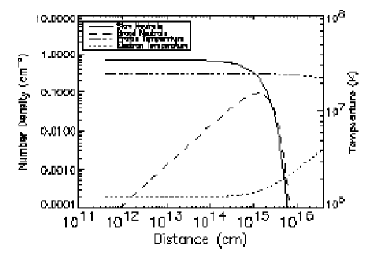
The temperatures are relatively steady throughout the simulation space of 4 $\times$ 10¹⁶ cm. However, the number of slow neutrals available to produce narrow emission drops off sharply within one ionization mean free path. The neutrals that are created from fast protons, the broad neutrals, are created and can exist further downstream than the slow narrow emission neutrals. Neutrals that become protons downstream quickly become thermalized with the hot downstream population. This implies all of the narrow emission comes from just behind the shock front within one ionization mean free path whereas the broad emission is more dispersed spatially.

A neutral particle is chosen randomly from this distribution and is tracked starting at the shock front shown as x=0 in Figure 4.3. A random thermal velocity is chosen from a gaussian distribution and assigned to the neutral particle. Time and distance are incremented and the probability of each of the three interactions (ionization, excitation, or charge transfer) are calculated.

Figure 4.3: The initial setup of the neutral model. There are four mean free path of length on either side of the shock. The

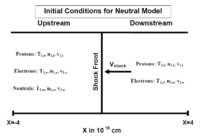
Although the interaction of neutrals with the shock front is the driving cause of the simulations, many factors contribute to this interaction. Detailed in Table 4.1, the shock speed, neutral fraction, magnetic field and orientation, and the degree of temperature equilibration between electrons and protons, $\alpha$, are varied to study the heating with respect to neutrals at the shock front.

Table 4.1: Summary of Parameters Studies for Neutral Simulation

Parameter	Value
Speed (km s-1)	300, 500, 1000, 1500, 2000, 2500, 3000
Neutral Fraction	0.2, 0.3, 0.5, 0.9
Magnetic Field (Gauss)	3 $\times$ 10-6
Magnetic Angle (Degrees)	0, 90, 45
$\frac{T_{e}}{T_{p}}$	0.1,0.5,0.9

4.3 Atomic Interactions

Three atomic interactions or a lack of interaction were possible for a particle at each time step: ionization, charge transfer, H$\alpha$ emission (excitation), or simple transport with no atomic processes taking place. The atomic interaction was then chosen by a Monte Carlo method based on the calculation of the probabilities of each of the three atomic interactions.

In general, the probability that a specific atomic process could take place is defined as

$$P=tn\sigma v$$ (4.2)

where
n=number density of target particles
t=time (time step in the model)
$\sigma$=cross section
v=velocity of particle.

To calculate the atomic rates of these interactions, several sources were used. For many of the rates, direct numerical integration over two Maxwellian distributions was preformed by Laming et al. (1996) and Laming (1990) to find the cross section of the interaction.

The charge transfer or electron capture reaction is as follows:

$$H^{+}+H\rightarrow H+H^{+}.$$ (4.3)

Charge transfer occurs between fast protons and slow neutrals or slow protons and fast neutrals. For charge transfers occurring downstream of the shock and charge transfer between a slow neutral and a fast proton, data from the Laming et al. (1996) and Laming (1990) papers were used.

For upstream charge transfer, the calculation for the cross sections were taken from the Redbook Atomic Data Tables (Barnett et al., 1990). The authors used a Chebyshev fitting method to fit experimental atomic data for this interaction. The minimum energy of an incoming proton is E_min=1.28 $\times$ 10^-1 eV/amu with a maximum incoming proton energy of E_max=6.3 $\times$ 10⁵ eV/amu. This encompasses the entire energy range of interest for this simulation. This cross section was then multiplied by the velocity and the density of the target particles in order to obtain a rate.

Ionization of a hydrogen atom in the simulation can occur by a interaction with either a proton or an electron, as shown by Equations 4.4 and 4.5.

$$H+H^{+}\rightarrow 2H^{+}+e^{-}$$ (4.4)

or by electrons

$$H+e^{-}\rightarrow H^{+}+2e^{-}$$ (4.5)

The reaction rate for ionization by a proton upstream when the thermal velocity of the ambient protons are small is given by Fang et al. (1995). The rate for ionization by an electron is taken from Scholz and Walters (1991). The downstream ionization rate was calculated from the Laming et al. papers.

The excitation of protons to produce the Balmer $\alpha$ line emission involves the transition of a hydrogen atom from the ground state to an excited state and the subsequent decay back to the ground state with the emission of a photon, h$\nu$.

$$H+e^{-}\rightarrow H^{*}+e^{-}\rightarrow H+h\nu$$ (4.6)

$$H+p^{+}\rightarrow H^{*}+p^{+}\rightarrow H+h\nu$$ (4.7)

For the excitation of a slow neutral downstream, the rates were taken from the Laming et al. papers. Excitation could also occur of a fast neutral. The probability that this excitation would occur again used the Laming et al. papers. Upstream, excitation of a slow neutral can occur. The rate for excitation by an electron into the 3p state and the combined 3s and 3d states are taken from Callaway (1994).

Once these probabilities were calculated at a specific location and time, they were fed into a subroutine that used a Monte Carlo algorithm to choose the interaction. Each interaction was then recorded and the velocity of the particle was modified. If the particle was ionized, it was assumed to leave the system and was no longer tracked because the new proton will quickly thermalize with the downstream plasma. Downstream of the shock, if the particle was excited the emission was recorded but the velocity left unchanged. If charge transfer occurred the proton that was created is assumed to quickly thermalize with the downstream plasma and is not tracked. The fast neutral produced by the downstream charge transfer was the particle that was followed.

Upstream of the shock, H$\alpha$ emission did not affect the velocity. Ionization or charge exchange with a fast neutral created a fast proton upstream. This was then tracked to understand the preheating of the plasma that could occur as described in the next section.

4.4 Upstream Precursor Generated By Fast Neutrals

When a proton undergoes charge exchange downstream, it becomes a fast neutral. This fast neutral, if oriented correctly, can pass through the shock front upstream without interacting with the magnetic field. There is a possibility that the fast neutral will be ionized or charge transfer and therefore become a fast proton upstream. As this fast proton travels upstream, it heats the surrounding environment. According to Spitzer (1956), Equation 4.8 describes the rate that a fast particle loses energy as

$$\frac{dE}{dt}=-\frac{m\omega^{2}}{t_{s}}$$ (4.8)

where
$\omega$=velocity of the particle
m=mass of particle
t_s=time for energy exchange by Coulomb collisions

This is the basis of a neutral precursor. The amount of heat is calculated based not only on Coulomb collisions, but also on the generation of Lower Hybrid waves by the velocity component due to gyration about the magnetic field. Lower Hybrid waves have been studied extensively in the heliosphere as a source of heating (Cairns and Zank, 2002; Shapiro et al., 1998a). As studied by Shapiro et al. (1998b) if there are electrons present they are heated by the lower hybrid waves if the Alfvenic velocity was less than the gyration speed. The energy deposited upstream was then recorded. The energy that is deposited due to wave interaction contributes to the thermal energy of the electrons. The Coulomb heating is assumed to increase the thermal energy of the protons.

4.5 Results of Simulations

Using a specific example, the atomic reactions were plotted versus distance from a parallel shock front in Figure 4.4. The initial neutral fraction is 30$\%$, the shock speed was 3000 km s^-1 and $\alpha$ is 0.1.

Figure 4.4: Atomic interactions versus distance from the shock front for a 3000 km s^-1 shock with 30 $\%$ neutral fraction and $\alpha$=0.1 in a parallel shock. The shock is at x=0, upstream is negative x and downstream is the positive x direction.

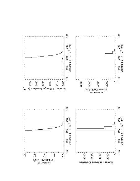
The ionization of the neutrals is within one ionization mean free path of the shock front. The ionization drops off sharply after the shock. The number of charge transfers also drops off sharply downstream of the shock. The broad excitation is centered on the shock front. In this example, there are 2000 interactions upstream of the shock, which is 2% of the total neutrals, (1$\times$10⁵), examined in the code. The narrow emission falls off quickly downstream and no emission is seen upstream.

In addition to keeping track of the interactions versus distance from the shock front, the broad to narrow ratios versus shock speed for each angle were plotted in Figures 4.5 - 4.7. Each plotting symbol corresponds to specific neutral fraction.

Figure 4.5: Plot of the broad to narrow intensity ratio versus shock speed for a parallel shock and $\alpha$=0.1. Variations in pre-shock neutral density is shown for 20%, 30%, 50% and 80% as detailed in the legend.

Figure 4.6: Plot of the broad to narrow intensity ratio versus shock speed for a 45 degree shock and $\alpha$=0.1. Variations in pre-shock neutral density is shown for 20%, 30%, 50% and 80% as detailed in the legend.

Figure 4.7: Plot of the broad to narrow intensity ratio versus shock speed for a perpendicular shock and $\alpha$=0.1.Variations in pre-shock neutral density is shown for 20%, 30%, 50% and 80% as detailed in the legend.

Figure 4.5 plots the broad to narrow intensity ratio for $\alpha$=0.1 for a parallel shock. Although overall the intensity ratios decrease with increasing shock speed, very little difference is seen between the various neutral fractions. The slowest shock studied with a velocity of 300 km sec^-1 was the most efficient producer of the broad component. Almost 12% of the neutrals came back upstream in this study. The high amount of neutrals were then available for creation of a broad component. Figure 4.6 plots the intensity ratio for a 45 degree shock. The overall trend of the intensity ratio to decrease with increasing shock speed still holds true. However, at this angle, the various neutral fractions do affect the intensity ratio. The perpendicular plot, Figure 4.7, is similar to the parallel plot as they both indicate that the slowest shocks are most effective in producing broad emission. This is due to the higher charge transfer rate and lower ionization rate at the shock speed and neutral fraction.

4.6 Discussion

By varying the parameters of the study, the relative importance of each parameter can be examined as to their contribution to the formation of a broad and narrow component of the H$\alpha$ emission.

4.6.1 Pre-shock neutral fraction

The pre-shock neutral fraction was varied from 20$\%$ to 80 $\%$. At high speeds, v_shock $\geq$ 2000, the intensity ratio drops because the charge transfer cross section declines. The neutral fraction did not affect the intensity ratios for large shock speeds, indicating the decrease in charge transfer cross section has a larger effect than the number of neutrals. The intensity ratios were affected by the neutral fraction when the shock speed was below 500 km sec^-1.

Lim and Raga (1996) did not find a large variation for a small neutral fraction. However, they did not account for magnetic interaction of the ratio of electron to proton temperature which we will now examine.

4.6.2 Electron and Proton Equilibration

The ratio of electron to proton temperature, $\alpha$, plays a key role in the resulting broad to narrow intensity ratio. From the previous Figures, Figures 4.5 - 4.7, $\alpha$=0.1 shows little variation in the broad to narrow intensity ratio. However, when the electron temperature is closer to the proton temperature the broad to narrow ratio versus shock speed varies. The intensity ratios increase until the shock speed is 1500 km s^-1 and then the ratios decreases as seen in Figures 4.8 - 4.13.

Figure 4.8: Plot of the broad to narrow intensity ratio versus shock speed for a parallel shock and $\alpha$=0.5.

Figure 4.9: Plot of the broad to narrow intensity ratio versus shock speed for a 45 degree shock and $\alpha$=0.5.

Figure 4.10: Plot of the broad to narrow intensity ratio versus shock speed for a perpendicular shock and $\alpha$=0.5.

Figure 4.11: Plot of the broad to narrow intensity ratio versus shock speed for a parallel shock and $\alpha$=0.9.

Figure 4.12: Plot of the broad to narrow intensity ratio versus shock speed for a 45 degree shock and $\alpha$=0.9.

Figure 4.13: Plot of the broad to narrow intensity ratio versus shock speed for a perpendicular shock and $\alpha$=0.9.

As was the case in the previous section, when a shock reaches velocities higher than 2000 km s^-1, the cross section for charge transfer for protons over 2 keV drops dramatically causing fewer broad emissions to be produced.

4.6.3 Magnetic Angle Effects

The orientation of the magnetic field to the shock normal has been shown in the previous chapters to play a role in heating of ions as the shock passes. Three orientations were examined in the neutral simulation, $\theta$=0, 45, 90. These angles were chosen to simulate a parallel, quasi-perpendicular, and perpendicular shock. The orientation of the magnetic field as in the parallel shock case can aid in a particle escaping upstream, whereas a perpendicular shock would be more likely to prohibit the motion of particles upstream. Each angle did produce different broad to narrow ratios, although very little difference was seen between the parallel and perpendicular cases. The parallel shock in general consistently produced the highest broad to narrow ratios for a given speed and neutral fraction. The difference in heating varied greatly between the perpendicular and parallel shock. This will be discussed in a following section.

4.6.4 Effect of Shock Speed on Neutral Signatures

From past observations of supernova remnants, Table 4.2 was constructed. Shock speed is the one factor that is readily available for comparison. As seen in the previous sections, many factors influence the intensity ratios. The shock speed changes this ratio significantly when the shock speed is greater than 1500 km s^-1. Beyond this shock speed, the intensity ratio varies little yet decreases with increasing shock speed.

The supernova remnants in Table 4.2 fall within the range of values for the broad to narrow intensity ratio found through this simulation. Further study would make this a useful tool for predicting interactions and possibly even magnetic angle and neutral fraction.

Table 4.2: Summary of Broad to Narrow Intensity Ratios for H$\alpha$

Remnant	Ratio	vshock	Model Ratio
Tycho	1.08$\pm$0.16	1800$\pm$100a,b	1.04-2.4
SN1006	0.73$\pm$0.06	2890$\pm$100c	0.47-1.1
0519-69.0	0.8 $\pm$0.2	1380$\pm$200b	1.0-1.4
0548-70.4	1.1$\pm$0.2	780$\pm$110 b	1.0-1.4

a) Kirshner et al. (1987)(b) Smith et al. (1991) (c) Ghavamian et al. (2002)

4.6.5 Pre-Heating by Neutrals

The simulation presented here set out to answer questions about the pre-heating that could occur with a neutral population present at a collisionless shock front. It could easily be assumed that as the number of neutrals increases the heating would also increase. In the perpendicular and parallel cases, little variance was seen in the heating based on neutral fraction. The one parameter that effected heating was the degree of thermal equilibrium between electrons and protons. A magnetic orientation of 45 degrees displayed a spread of heating versus initial neutral fraction.

In the case of $\alpha$=0.1, there is a decrease in preheating with increasing shock velocities. The lowest pre-shock neutral fraction, 20$\%$ has the most relative pre-heating. For the cases of $\alpha$=0.5 and 0.9, similar trends of increasing heating with decreasing initial neutral fraction present. If the electrons are cooler than protons and there are few neutrals, the heating mechanism is relying on shock speed to increase heating. Whereas when the electrons are closer in temperature to the protons, the shock speed is not the dominate mechanism available for heating.

Figure 4.14: Plot of the upstream heating versus shock speed for a 45 degree shock and $\alpha$=0.1.

Figure 4.15: Plot of the upstream heating versus shock speed for a 45 degree shock and $\alpha$=0.5.

Figure 4.16: Plot of the upstream heating versus shock speed for a 45 degree shock and $\alpha$=0.9.

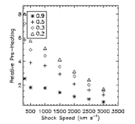
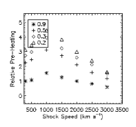
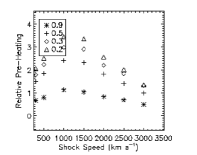
To answer some of the fundamental questions about neutrals at the shock front, a summary of the finding for heating of all shocks follows. The number of particles that made it upstream and were available to perform pre-heating was about 9$\%$ of the total particle simulation with as low as 2% and as high as 14% of the particles preheating the shock. The heating varied based on magnetic orientation of the shock. Per heating interaction, the particles in the parallel shock gave up the most energy followed by a quasi perpendicular shock. The perpendicular shock displayed the least amount of preheating.

4.7 Conclusions

Neutrals play a key role in the observational spectral from shocks associated with supernova remnants. The degree of temperature equilibrium between electrons and protons played the largest role in the outcome of the broad to narrow intensity ratios. However, once the degree of equilibrium approaches one, the shock speed and the neutral fraction were more effective in changing and modifying the intensity ratio. The magnetic angle did play a role in heating yet further study is necessary to conclude a trend.

A full 3-D MHD particle simulation would be ideal to understand the physics of the neutrals at the shock front. However, using this 2-D model observed data could be simulated. Future work could include the shock going through a non-homogenous or clumpy material. In addition, the magnetic field plays a key role in particle transport that the study of magnetic inhomogeneities and structure would also improve the simulations as well as MHD waves and instabilities that are available to heat the plasma. Future work could include heavier ions as they would act as another fluid in the simulations. The interaction of heavy atoms as neutrals or ions at low charge states would be an interesting application of the code.

Chapter V Conclusions and Future Work

This thesis has performed the most comprehensive study to date of the heating of ions and neutrals in collisionless shocks. The heavy ion heating was examined in several different environments as a function of M_A, $\beta$, and magnetic field orientation. The heating based on mass fractionation was discussed in both supernova remnants and the shocks that propagate before a CME. The neutral population of a pre-shock plasma was also investigated to examine the atomic processes involved in the electromagnetic emission from a shock as well as to help interpret and understand the observed astronomical data from shocks. The integration of different measurements allows us to use the data to make predictions about magnetic field orientation and the magnetic energy present, which is key to understanding particle heating and acceleration.

5.1 Summary of Work

5.1.1 Supernova Remnant Shock Heating

In Chapter 2, the ion heating in SN1006 was examined using observations from the FUSE Satellite. Due to the faintness of the current observations only the OVI and the Ly-$\beta$ spectral lines were available to determine the less than mass proportional heating. Using past observations, the less than mass proportional heating was confirmed. The plasma $\beta$ of the SNR is $\sim$ 0.1 which is similar to that of the heliospheric shocks studied indicating that the heating process is magnetically dominated. However, unlike the heliosphere the heavy ions in the supernova are less than mass proportionally heated.

Supernova remnants present many obstacles that make studying them difficult: distance from observation, few photons, no clear indication of magnetic orientation, etc. Although more observations and multi-wavelength studies could be integral to understanding the current data, this thesis examines the plasma physics of the heliosphere shocks and how we can apply the in situ measurements to understand the astronomical data. This study is opening new frontiers in understanding the magnetic field of an astronomical object by using shock heating data.

5.1.2 CMEs Heating

Chapter 3 dealt with in situ data taken from the collisionless shocks in front of Coronal Mass Ejections. Each shock was classified according to magnetic angle to the shock normal. The Mach number and the plasma beta were then examined for their effect on the ion heating. Quasi-perpendicular shocks were found to heat ions more than quasi-parallel shocks. The Mach number was not found to have a definitive effect on the heating.

Parallel shocks heated the ions less than the perpendicular shocks. The heating decreased with increasing $\beta$. A correlation of the decrease in magnetic energy that is indicated by an increasing $\beta$ with the decrease in heating implies that magnetic effects are dominant in the heating process. A parallel shock was also compared to a multi-fluid derivation of the Rankine Hugoniot conditions. For all but the energy term, the ion data matched the expected results. The energy term does include a potential which could be derived from the difference between the predicted and actual values.

Future observations in the heliosphere of CME shocks will be conducted by STEREO. The Solar TErrestrial RElations Observatory (STEREO) Mission will explore the 3-D shock structure, which is of importance to the evolution of the particle distributions. The study of the deviations of the particle distributions from Maxwellian is of interest to understand the heating, acceleration, and relaxation processes in the solar wind.

An interesting consequence of this thesis is the ability to use in situ heliospheric data to make predictions and further examine astronomical data. One such case is the prediction of the plasma $\beta$ for the supernova environment based on the observed heating. A strong correlation of decreasing ion heating with increasing plasma $\beta$ was found. Using the data from the Supernova 1006 study and the CME shock study for parallel shocks, Figure 5.1 was created. The northwest region of SN1006 is assumed to have a parallel shock due to the galactic magnetic field orientation. The x-axis is the plasma $\beta$. The y-axis is the ratio of upstream heating of an ion to a proton. A linear fit to the CME data is shown as the solid black line. The heating seen in the supernova is the dashed horizontal line. Where the dashed line meets the fit of the data is the predicted plasma $\beta$ for the supernova. The prediction for the plasma $\beta$ is 0.77. This varies from the $\beta$ calculated from the densities obtained from observations. The value is a factor of 7 higher than the calculated $\beta$. The higher value coincides with the lack of magnetic energy in the region. In the future, heliospheric trends can be utilized to obtain a range of probable $\beta$ values for supernova remnant shocks and other astronomical collisionless shocks.

Figure 5.1: Downstream Temperature Ratio versus Plasma $\beta$ for parallel shocks. The x-axis is plasma $\beta$. The y-axis is the ratio of downstream ion temperature to proton temperature. The dashed horizontal line is the value for SN1006. The solid line is a fit to the heating of the parallel shocks in the study. The intersection of these two lines at $\beta$ =0.77 is the predicted plasma $\beta$ for the supernova.

5.1.3 Neutral at the Shock Front: Source of Heating

Chapter Four explored the role of neutrals at a collisionless shock front. Neutrals are important for producing emission lines as well as the atomic interactions and our understanding of these interactions. The degree of thermal equilibrium between protons and electrons played a surprising role in the broad to narrow intensity ratios.

One important factor was found to be the orientation of the magnetic field for the ratio of broad to narrow components. Using the broad to narrow intensity ratio from SN1006, we try to predict the magnetic orientation of the shocks in the northeast and northwest. For SN1006, an $\alpha$ of $\sim$0.1 is observed(Vink et al., 2003). Using Figures 4.5 -4.7 and the shock velocity from Table 4.2, one could estimate that the shock is a quasi-perpendicular shock. This is what the northeast rim of SN1006 would be if the assumptions about the Interstellar magnetic field orientation is correct. This also is in line with the heating seen in the CME work. The northeast rim of SN1006 is the region where X-ray emission is bright as well as the observations of gamma rays were reported (Bamba et al., 2003).

This proves to be an interesting tool. Magnetic fields and their orientation are notoriously difficult to measure. If the intensity ratio and a measurement of the electron and proton temperatures can be used to at least create a limit to the magnetic parameter, much progress can be made in understanding acceleration methods that rely on magnetic angle.

5.2 Collisionless Shocks in the Interstellar Medium

As we have seen, collisionless shocks that form from interactions within the interstellar medium (ISM) heat the ISM in ways that are not well understood. As this dissertation has shown, shocks can reveal many characteristics of plasma interactions such as temperature, density, magnetic field strength, and ionization state. Our understanding of the physics of these heating mechanisms is increased through the comparative study of these shocks. For future work there are three main prongs of work that would complement each other: analysis of multi-wavelength observation shock data, theoretical shock characterization of the system, and Magnetohydrodynamics (MHD) modeling of the systems using the BATS-R-US 3-D MHD code. This unique blend of theory, observation, and modeling gives a comprehensive view of the shock and how it interacts and subsequently heats the plasma.

5.2.1 Analysis of Observational Shock Data

Supernova remnants, CMEs, and non-relativistic jets of stellar systems all have collisionless shocks. By looking at a broad range of shocks both in the heliosphere and in astrophysical systems, we study a larger range of parameters, such as velocity and density, resulting in constraints and improved input for future theoretical models. To increase our understanding of shock heating use of multi-wavelength data is necessary.

In this sense, radio observations of the jets and shocks would prove useful. At radio wavelengths, synchrotron emission from electrons will give a rough estimate of non-thermal electron density. If an estimate of the energy and mass outflow of the jets is obtained, the mass infall rate can be estimated. Supernovas such as Tycho, Kepler, and SN1006 have been observed in the x-ray and radio. The radio and X-ray data from the SNR could be used to study shock trends such as the evolution of temperature with time, velocity distribution of the particles and the broad to narrow components of H$\alpha$ and shock emission.

The first data set is of Cygnus Loop, the middle aged supernova remnant with a shock speed of $\sim$350 km s^-1. The remnant was observed with the MMT long slit spectrograph in the 3300-5000 Å  wavelength range. After an initial review of the data, several lines are available for study, Ne III, Ne V, OII and Balmer H-$\beta$. The higher order H lines will more accurately pinpoint the temperature and ionization state of the plasma. The data will afford a mass-to-charge ratio versus temperature calculation as long as the radiation of the shock is low. The mass-to-charge ratio played a key factor in determining the heating in shocks in the heliosphere in Chapter 3. Using the varying speed and strength of prior observations of supernova, a trend in the velocity versus the mass-to-charge ratio can be calculated.

Another interesting data set is a Chandra observation of the jets of the symbiotic stars of R Aquarii. Chandra x-ray data show magnetic interactions leading to accretion mechanisms and acceleration of the plasma outward from the star. More observations of the system are planned as it reveals an evolution of the jet with time. The jets have been observed in the radio (Stark et al. 1992) as well as the x-ray wavelengths. The current observations show a collimated flow with a shock forming where the jet meets the ISM. This system will be of key interest to the MHD modelling efforts.

Solar wind data containing many shocks with varying parameters will be obtained from the Advanced Composition Explorer (ACE) satellite. ACE is situated 240 R_E upstream of the Earth. We will examine the data in an effort to improve the understanding of the energetics of the solar wind. This also allows for an examination of heavier ions such as Si and Mg to determine the role of heating minor ions in a shock front. The solar data set allows for a study of the distribution of thermal speeds of ions at the shock front which could be non-Maxwellian leading to information on the number of high energy particles available for acceleration processes. The root mean square of the magnetic field can be compared to thermal energy to test for turbulence.

5.2.2 Theoretical Shock Characterization

The Rankine-Hugoniot(RH) conservation equations describe how the temperature, pressure, and density pre-shock (upstream) relates to the post-shock (downstream) temperature, pressure and density. Magnetic fields can be included in these conservation equations making them acceptable for use in systems where there is significant magnetic energy. Simplifications are made in many approximations used for shock analysis. Turbulence and viscosity are ignored, as well as the temperature difference between electrons and protons. In addition, the distribution of particles is generally assumed to be Maxwellian which can be far from reality in shocked astrophysical plasmas. These assumptions need to be re-explored as the interpretation for more precise data is needed. A multi-fluid approach like that of Burgi (1991), is needed to successfully interpret shock data.

Because these shocks are expanding into a neutral ISM, the model previously developed in Chapter 4 to study neutral interaction will be used to characterize the shock. The Monte Carlo code will be updated to include the effect of turbulence, viscosity, and temperature differences between species in the plasma. In addition, cosmic ray acceleration based on these shocks will be considered by studying the ion heating and the distribution functions of particles.

Most of the work done on shock heating originates from heliospheric data. Advances made in understanding shock heating in the heliosphere will be applied to observations outside the heliosphere. A coherent scheme will be built to convert from the particle detection methods in the heliosphere to the photon detection methods in astronomy to further the ability to compare the shocks and other types of data. Results from the revised Monte Carlo code will show possible emission mechanisms and intensities of lines which will quantify the density, pressure and temperature upstream and downstream. The results of the study of the emission mechanisms and data correlation will determine the most important observable in a shock front and therefore enhance modelling including these parameters. This will also allow us to focus our observations on the characteristics that will lead to the most fruitful data set. Feedback from the analysis of observations will improve the theoretical model.

5.2.3 MHD Modelling Using BATS-R-US

BATS-R-US , a block adaptive grid code, is a first principles MHD model that has been used to study the Earth’s magnetosphere, comets, and the heliosphere. This code can be used for any system that satisfies the MHD conservation equations. Using the MHD model, simulations of the observed characteristics of the jet-shock-ISM system will be performed and therefore be able to better constrain the temperature, density, and magnetic field present. The first simulation will be of the R Aquarii binary system. Chandra observations reveal two x-ray jets coming from the system (Kellogg et. al. 2001). R Aquarii is a symbiotic star system made up of a Mira-type mass-losing variable with a white dwarf companion. The system is relatively close to the Earth ( 200 pc) facilitating the study of these jets. The system’s orbit is highly inclined (70 degrees) to the line of sight with the accretion disk of the hot companion edge-on. The magnetic field is assumed to be a dipole field that is aligned with the axis of rotation of the white dwarf, which for simplicity, is taken to be perpendicular to the plane of the orbit. The simulations would start with the simplest assumptions of a three species plasma (protons, electrons, and neutrals). The input into the code will require the density, temperature and magnetic field of the white dwarf and the accretion disk. The resulting output would be the jet density, temperature and magnetic field. The output will also contain a time evolution of the system. This model will place tight limits on the temperatures and densities originally needed to produce the jet therefore constraining the temperature and density of the binary system. BATS-R-US has been used to simulate other jet systems. A jet sheet that is formed at the intersection of the heliosphere and the ISM has been found by modeling done by Opher et al. 2004. These high resolution models simulate the pressure, temperature, speed, and magnetic field of the system. In addition, supernova shocks of SN1006 and Cygnus loop will be simulated to determine the debated magnetic field orientation and density. Through this similarity study, BATS-R-US can be used as a predictive tool for shocks and jets.

Solar Physics has a plethora of in situ data and physical models backing up the data analysis. Astronomical observational capabilities are beginning to be able to resolve objects with sizes similar to that of the heliosphere. However, it is still a great challenge to understand the physics based on the emission mechanisms for the few photons observed. In summary, this research would use multi-wavelength observations to study shocks, use these observations to better model the system and then use an advanced 3-D MHD code, BATS-R-US to simulate the time evolution of the system. Eventually this research will use the combination of a shock physics model and the MHD code to predict and analyze observed data. Future studies will use the MHD code as a predictive and analytic tool for the jets associated with HH objects, protoplanetary disks, comets, coronal mass ejections, and supernova shocks. The completion of this project will give me a solid foundation to work to bridge astrophysics and space physics.

5.3 Future of Collisionless Shock Research

The cross disciplinary mix of physics, astronomy, and space science can only help to further each of the disciplines. This thesis used a unique combination of systems from each of the disciplines in order to understand the heating of heavy ions and neutrals in collisionless shocks. This facilitates the advancement of plasma astrophysics and the understanding of the cosmic ray puzzle.

Future work in collisionless shock research lies in a multi-wavelength, multi-system approach. By using the models already in existence and theories from different subfields of astrophysics, the understanding of collisionless shock physics will increase dramatically.

ABSTRACT

ION HEATING IN COLLISIONLESS SHOCKS IN SUPERNOVAE AND THE HELIOSPHERE

by

Kelly Elizabeth Korreck

Co-Chairpersons: Thomas H. Zurbuchen and John C. Raymond

Collisionless shocks play a role in many astrophysical phenomena, from coronal mass ejections (CMEs) in the heliosphere to supernova remnants. Their role in heating and accelerating particles is well accepted yet the exact mechanism for ion heating is not well understood. Two systems, CMEs and supernova remnants, were examined to determine the heating of heavy ions as they pass through collisionless shocks thus providing a seed population for cosmic ray acceleration processes. Three parameters are examined, the plasma beta, the Mach number of the shock and the magnetic angle of the shock. CMEs heat heavy ions preferentially. This is in contrast to the supernova data which shows less than mass proportional heating. In addition to these studies, heating in astrophysical systems involves neutral atoms. A Monte Carlo model simulated neutral particles as they pass through the shock. Neutrals can create a precursor to the shock additionally heating the plasma. This work uses in situ data from the heliosphere to study astronomical systems because of common shock properties is a unique way to study magnetic components of shocks remotely.

References

- Alfvén (1945) Alfvén, H.: 1945, MNRAS 105, 3
- Anderson et al. (2003) Anderson, B., Sankrit, R., and Dupuis, J.: 2003, FUSE Observer’s Guide
- Bale et al. (2002) Bale, S. D., Hull, A., Larson, D. E., Lin, R. P., Muschietti, L., Kellogg, P. J., Goetz, K., and Monson, S. J.: 2002, ApJ, Lett. Ed. 575, L25
- Bamba et al. (2003) Bamba, A., Yamazaki, R., Ueno, M., and Koyama, K.: 2003, ApJ 589, 827
- Barnett et al. (1990) Barnett, C. F., Hunter, H. T., Fitzpatrick, M. I., Alvarez, I., Cisneros, C., and Phaneuf, R. A.: 1990, NASA STI/Recon Technical Report N 91, 13238
- Baumjohann and Treumann (1997) Baumjohann, W. and Treumann, R. A.: 1997, Basic space plasma physics, London: Imperial College Press, —c1997
- Belcher et al. (1993) Belcher, J. W., Lazarus, A. J., McNutt, R. L., and Gordon, G. S.: 1993, J. Geophys.Res. 98(17), 15177
- Berdichevsky et al. (1997) Berdichevsky, D., Geiss, J., Gloeckler, G., and Mall, U.: 1997, J. Geophys.Res. 102, 263
- Burgi (1991) Burgi, A.: 1991, J. Geophys.Res. 96(15), 17689
- Cairns and Zank (2002) Cairns, I. H. and Zank, G. P.: 2002, Geophys. Res. Lett. 29, 47
- Callaway (1994) Callaway, J.: 1994, Atomic Data and Nuclear Data Tables 57, 9
- Cane and Richardson (2003) Cane, H. and Richardson, I.: 2003, J. Geophys.Res. 108, 1156
- Carroll and Ostlie (1996) Carroll, B. and Ostlie, D.: 1996, An Introduction to Modern Astrophysics, Addison Wesley
- Chandrasekhar (1984) Chandrasekhar, S.: 1984, Science 226, 497
- Charles and Seward (1995) Charles, P. and Seward, F.: 1995, Exploring the X-ray Universe, Cambridge University Press
- Chen (1984) Chen, F.: 1984, Introduction to Plasma Physics and Controlled Fusion, Plenum Press
- Chevalier et al. (1980) Chevalier, R., Kirshner, R., and Raymond, J.: 1980, ApJ 235, 186
- Chevalier and Raymond (1978) Chevalier, R. and Raymond, J.: 1978, ApJ 225, L27
- Chevalier (1982) Chevalier, R. A.: 1982, ApJ, Lett. Ed. 259, L85
- Draine (1980) Draine, B.: 1980, ApJ 241, 1021
- Ellison and Reynolds (1991) Ellison, D. and Reynolds, S.: 1991, ApJ 382, 242
- Fang et al. (1995) Fang, C., Feautrier, N., and Henoux, J.-C.: 1995, A&A 297, 854
- Finland (1998) Finland, S. P. G. O.: 1998, Space Physics Textbook, spaceweb@oulu.fi
- Fisk et al. (1974) Fisk, L., Kozlovsky, B., and Ramaty, R.: 1974, Astrophys. Lett. 190, L35
- Fisk (2003) Fisk, L. A.: 2003, Journal of Geophysical Research (Space Physics) 108(A4), 7
- Flower et al. (1985) Flower, D., des Forets, G. P., and Hartquist, T.: 1985, MNRAS 216, 775
- Forbes (2000) Forbes, T.: 2000, J. Geophys.Res. 105(A10), 23153
- Fuselier and Schmidt (1997) Fuselier, S. A. and Schmidt, W. K. H.: 1997, J. Geophys.Res. 102(11), 11273
- Garrard et al. (1998) Garrard, T. L., Davis, A. J., Hammond, J. S., and Sears, S. R.: 1998, Space Science Reviews 86, 649
- Ghavamian et al. (2002) Ghavamian, P., Winkler, P., Raymond, J., and Long, K.: 2002, ApJ 572, 888
- Gloeckler et al. (1998) Gloeckler, G., Cain, J., Ipavich, F. M., Tums, E. O., Bedini, P., Fisk, L. A., Zurbuchen, T. H., Bochsler, P., Fischer, J., Wimmer-Schweingruber, R. F., Geiss, J., and Kallenbach, R.: 1998, Space Science Reviews 86, 497
- Gombosi (1999) Gombosi, T. I.: 1999, Physics of the Space Environment, Physics of the Space Environment, ISBN 052159264X, Cambridge University Press, 1999.
- Goodman (1992) Goodman, R.: 1992, LAKOTA STAR KNOWLEDGE: STUDIES IN LAKOTA STELLAR THEOLOGY 2nd Edition, Sinte Gleshka University Press, information at P.O. Box 490 Rosebud SD 57570-0490 605-856-2368
- Gosling et al. (1997) Gosling, J. T., Bame, S. J., Feldman, W. C., McComas, D. J., Riley, P., Goldstein, B. E., and Neugebauer, M.: 1997, Geophys. Res. Lett. 24, 309
- Gosling et al. (1974) Gosling, J. T., Hildner, E., MacQueen, R. M., Munro, R. H., Poland, A. I., and Ross, C. L.: 1974, J. Geophys.Res. 79(18), 4581
- Habbal et al. (1997) Habbal, S. R., Woo, R., Fineschi, S., O’Neal, R., Kohl, J., Noci, G., and Korendyke, C.: 1997, ApJ, Lett. Ed. 489, L103+
- Hefti (1998) Hefti, S.: 1998, SWICS/ACE Technical Note
- Hester et al. (1994) Hester, J. J., Raymond, J. C., and Blair, W. P.: 1994, ApJ 420, 721
- Hetherington (1996) Hetherington, B.: 1996, A chronicle of pre-telescopic astronomy, John Wiley and Sons., Paul Charbonneau,Great Moments in the History of Solar Physics copyright2000
- Horowitz and Li (1999) Horowitz, C. J. and Li, G.: 1999, Physical Review Letters 82, 5198
- Jones and Pye (1988) Jones, L. and Pye, J.: 1988, MNRAS 238, 567
- Kahler (1992) Kahler, S. W.: 1992, Ann. Rev. A&A 30, 113
- Kaufmann (1991) Kaufmann, W.: 1991, Universe 3rd. Ed., W.H. Freeman and Company, New York
- Kennel et al. (1985) Kennel, C. F., Edmiston, J. P., and Hada, T.: 1985, Washington DC American Geophysical Union Geophysical Monograph Series 34, 1
- Kirshner et al. (1987) Kirshner, R., Winkler, P., and Chevalier, R.: 1987, ApJ 315, L135
- Korreck et al. (2004) Korreck, K. E., Raymond, J. C., Zurbuchen, T. H., and Ghavamian, P.: 2004, ApJ 615, 280
- Laming (1990) Laming, J. M.: 1990, ApJ 362, 219
- Laming (2004) Laming, J. M.: 2004, ApJ 604, 874
- Laming et al. (1996) Laming, J. M., Raymond, J. C., McLaughlin, B. M., and Blair, W. P.: 1996, ApJ 472, 267
- Lee and Wu (2000) Lee, L. and Wu, B.: 2000, ApJ 535, 1014
- Lee et al. (1987) Lee, L. C., Mandt, M. E., and Wu, C. S.: 1987, J. Geophys.Res. 92(11), 13438
- Lee et al. (1986) Lee, L. C., Wu, C. S., and Hu, X. W.: 1986, Geophys. Res. Lett. 13, 209
- Lembege et al. (2004) Lembege, B., Giacalone, J., Scholer, M., Hada, T., Hoshino, M., Krasnoselskikh, V., Kucharek, H., Savoini, P., and Terasawa, T.: 2004, Space Science Reviews 110, 161
- Leroy et al. (1982) Leroy, M. M., Winske, D., Goodrich, C. C., Wu, C. S., and Papadopoulos, K.: 1982, J. Geophys.Res. 87(16), 5081
- Lim and Raga (1995) Lim, A. and Raga, A.: 1995, MNRAS
- Lim and Raga (1996) Lim, A. and Raga, A.: 1996, MNRAS 280, 103
- Long et al. (2003) Long, K., Reynolds, S., and Raymond, J.: 2003, ApJ 586, 1162
- MacQueen (1980) MacQueen, R. M.: 1980, Royal Society of London Philosophical Transactions Series A 297, 605
- McComas et al. (1998) McComas, D. J., Bame, S. J., Barker, P., Feldman, W. C., Phillips, J. L., Riley, P., and Griffee, J. W.: 1998, Space Science Reviews 86, 563
- McKee and Ostriker (1977) McKee, C. F. and Ostriker, J. P.: 1977, ApJ 218, 148
- Moore et al. (1999) Moore, R. L., Falconer, D. A., Porter, J. G., and Suess, S. T.: 1999, ApJ 526, 505
- Moos et al. (2000) Moos, H. W., Cash, W. C., Cowie, L. L., Davidsen, A. F., Dupree, A. K., Feldman, P. D., Friedman, S. D., Green, J. C., Green, R. F., Gry, C., Hutchings, J. B., Jenkins, E. B., Linsky, J. L., Malina, R. F., Michalitsianos, A. G., Savage, B. D., Shull, J. M., Siegmund, O. H. W., Snow, T. P., Sonneborn, G., Vidal-Madjar, A., Willis, A. J., Woodgate, B. E., York, D. G., Ake, T. B., Andersson, B.-G., Andrews, J. P., Barkhouser, R. H., Bianchi, L., Blair, W. P., Brownsberger, K. R., Cha, A. N., Chayer, P., Conard, S. J., Fullerton, A. W., Gaines, G. A., Grange, R., Gummin, M. A., Hebrard, G., Kriss, G. A., Kruk, J. W., Mark, D., McCarthy, D. K., Morbey, C. L., Murowinski, R., Murphy, E. M., Oegerle, W. R., Ohl, R. G., Oliveira, C., Osterman, S. N., Sahnow, D. J., Saisse, M., Sembach, K. R., Weaver, H. A., Welsh, B. Y., Wilkinson, E., and Zheng, W.: 2000, ApJ, Lett. Ed. 538, L1
- Murthy and Henry (1995) Murthy, J. and Henry, R.: 1995, ApJ 448, 848
- Ogilvie et al. (1980) Ogilvie, K. W., Bochsler, P., Geiss, J., and Coplan, M. A.: 1980, J. Geophys.Res. 85(14), 6069
- Otte et al. (2003) Otte, B., Dixon, W., and Sankrit, R.: 2003, ApJ 586, L53
- Otte et al. (2004) Otte, B., Dixon, W. V. D., and Sankrit, R.: 2004, Astrophys. Lett. 606, L143
- Papadopoulos (1985) Papadopoulos, K.: 1985, in Advances in Space Plasma Physics, pp 289–+
- Pye et al. (1981) Pye, J. P., Pounds, K. A., Rolf, D. P., Smith, A., Willingale, R., and Seward, F. D.: 1981, MNRAS 194, 569
- Ray (1958) Ray, D. J.: 1958, The ALASKA SPORTSMAN, reprinted in AURORA BOREALIS The Amazing Northern Lights by S.I. Akasofu Alaska Geographic Volume 6 Number 2 1979
- Raymond et al. (1995) Raymond, J. C., Blair, W. P., and Long, K. S.: 1995, Astrophys. Lett. 454, L31+
- Reynolds (2004) Reynolds, S. P.: 2004, Advances in Space Research 33, 461
- Reynolds and Gilmore (1986) Reynolds, S. P. and Gilmore, D. M.: 1986, AJ 92, 1138
- Scholz and Walters (1991) Scholz, T. T. and Walters, H. R. J.: 1991, ApJ 380, 302
- Schweizer and Middleditch (1980) Schweizer, F. and Middleditch, J.: 1980, ApJ 241, 1039
- Sedov (1959) Sedov, L. I.: 1959, Similarity and Dimensional Methods in Mechanics, Similarity and Dimensional Methods in Mechanics, New York: Academic Press, 1959
- Shapiro et al. (1998a) Shapiro, V. D., Bingham, R., Dawson, J. M., Dobe, Z., Kellett, B. J., and Mendis, D. A.: 1998a, Physica Scripta Volume T 75, 39
- Shapiro et al. (1998b) Shapiro, V. D., Bingham, R., Dawson, J. M., Dobe, Z., Kellett, B. J., and Mendis, D. A.: 1998b, Physica Scripta Volume T 75, 39
- Smith et al. (1998) Smith, C. W., L’Heureux, J., Ness, N. F., Acuña, M. H., Burlaga, L. F., and Scheifele, J.: 1998, Space Science Reviews 86, 613
- Smith et al. (1991) Smith, R. C., Kirshner, R. P., Blair, W. P., and Winkler, P. F.: 1991, ApJ 375, 652
- Smith et al. (1994) Smith, R. C., Raymond, J. C., and Laming, J. M.: 1994, ApJ 420, 286
- Sonett and Abrams (1963) Sonett, C. P. and Abrams, I. J.: 1963, J. Geophys.Res. 68(17), 1233
- Spitzer (1956) Spitzer, L., J.: 1956, Physics of Fully Ionized Gases, Interscience Publishers, Inc.
- Stepanova and Kosovichev (2000) Stepanova, T. V. and Kosovichev, A. G.: 2000, Advances in Space Research 25, 1855
- Stone et al. (1998) Stone, E. C., Frandsen, A. M., Mewaldt, R. A., Christian, E. R., Margolies, D., Ormes, J. F., and Snow, F.: 1998, Space Science Reviews 86, 1
- Strom (1994) Strom, R. G.: 1994, A&A 288, L1
- Tanimori et al. (1998) Tanimori, T., Hayami, Y., Kamei, S., Dazeley, S. A., Edwards, P. G., Gunji, S., Hara, S., Hara, T., Holder, J., Kawachi, A., Kifune, T., Kita, R., Konishi, T., Masaike, A., Matsubara, Y., Matsuoka, T., Mizumoto, Y., Mori, M., Moriya, M., Muraishi, H., Muraki, Y., Naito, T., Nishijima, K., Oda, S., Ogio, S., Patterson, J. R., Roberts, M. D., Rowell, G. P., Sakurazawa, K., Sako, T., Sato, Y., Susukita, R., Suzuki, A., Suzuki, R., Tamura, T., Thornton, G. J., Yanagita, S., Yoshida, T., and Yoshikoshi, T.: 1998, Astrophys. Lett. 497, L25+
- Tennekes and Lumley (1972) Tennekes, H. and Lumley, J.: 1972, A First Course in Turbulence, The MIT Press
- Tidman (1969) Tidman, D. A.: 1969, in Plasma Instabilities in Astrophysics, pp 229–+
- Universe (2000) Universe: 2000, Myths: Tonatiuh, http://www.windows.ucar.edu Accessed December 4 2004
- van Ballegooijen and Martens (1989) van Ballegooijen, A. A. and Martens, P. C. H.: 1989, ApJ 343, 971
- Vasyliunas and Siscoe (1976) Vasyliunas, V. M. and Siscoe, G. L.: 1976, J. Geophys.Res. 81(10), 1247
- Vink et al. (2003) Vink, J., Laming, J. M., Gu, M. F., Rasmussen, A., and Kaastra, J. S.: 2003, Astrophys. Lett. 587, L31
- Wang and Sheeley (1990) Wang, Y.-M. and Sheeley, N. R.: 1990, ApJ 355, 726
- Willingale et al. (1996) Willingale, R., West, R. G., Pye, J. P., and Stewart, G. C.: 1996, MNRAS 278, 749
- Winkler et al. (2003) Winkler, P. F., Gupta, G., and Long, K. S.: 2003, ApJ 585, 324
- Woo and Habbal (1997) Woo, R. and Habbal, S. R.: 1997, Geophys. Res. Lett. 24, 1159
- Zertsalov et al. (1976) Zertsalov, A. A., Vaisberg, O. L., and Temnyi, V. V.: 1976, Cosmological Research 14, 257
- Zhao et al. (1991) Zhao, X., Ogilvie, K. W., and Whang, Y. C.: 1991, J. Geophys.Res. 96, 5437