Photometric observations from theoretical flip-flop models

Some active stars show a so-called flip-flop phenomenon in which the main spot activity periodically switches between two active longitudes that are 180° apart. In this paper we study the flip-flop phenomenon by converting results from dynamo calculations into long-term synthetic photometric observations, which are then compared to the real stellar observations. We show that similar activity patterns as obtained from flip-flop dynamo calculations, can also be seen in the observations. The long-term light-curve behaviour seen in the synthesised data can be used for finding new stars exhibiting the flip-flop phenomenon.

1 Introduction

In many active stars the spots concentrate on two permanent active longitudes which are $180^{\circ}$ apart. In some of these stars the dominant part of the spot activity changes the longitude every few years. This so-called flip-flop phenomenon was first reported by Jetsu et al. (jetsu1 (1991), jetsu2 (1993)) in the single, late type giant FK Com. Berdyugina & Tuominen (ber_tuo (1998)) reported periodic flip-flops between permanent active longitudes in four RS CVn binaries. Their results were confirmed in the case of II Peg by Rodonò et al. (rod (2000)). The persistent active longitude structures and flipping between two active longitudes have also been reported over the years based on photometric observation (e.g. Berdyugina et al. ber_lqhya (2002); Korhonen et al. kor4 (2002); Järvinen et al jarv (2005)) and on Doppler images (Berdyugina et al. ber2 (1998); Korhonen et al. kor_ff (2001)). After its discovery in cool stars, the flip-flop phenomenon has also been reported in the Sun (Berdyugina & Usoskin ber_sun (2003)). A review on the flip-flop phenomenon in cool stars and the Sun is given by Berdyugina (ber_ff (2004)).

In order to explain this phenomenon, a non-axisymmetric dynamo component, giving rise to two permanent active longitudes 180° apart, is needed together with an oscillating axisymmetric magnetic field. Fluri & Berdyugina (flu_ber (2004)) suggest also another possibility with a combination of stationary axisymmetric and varying non-axisymmetric components. Unfortunately, no simple dynamo mechanism is yet known for such a configuration. There are models with anisotropic $\alpha$-effect or a weak differential rotation, which could produce non-axisymmetric components, but only recently Moss (moss1 (2004), moss2 (2005)) reported coexisting mixed components with a differential rotation that depends on the distance to the rotation axis. This differential rotation configuration is a very plausible state for fast rotators. Also, a weak non-axisymmetric field coexisting with a dominant axisymmetric field, assuming a solar-like rotation law, was found by Moss (moss99 (1999)). This solution was not analysed for flip-flops, as the possibility of them being present on the Sun was not being discussed at that time. Flip-flop solutions for a rotation law similar to the solar one and anisotropic $\alpha$ have also been found by Elstner & Korhonen (elstner (2005)).

According to the calculations by Elstner & Korhonen (elstner (2005)) the shift of the spots in a flip-flop event is 180° only in some cases, mainly for the stars with thin convective zones. In stars with thick convective zones they found a shift that is close to 90°. Similar results were reported by Moss (moss2 (2005)). Recently, Oláh et al. (olah (2005)) re-analysed some of the old photometric observations of FK Com and found a flip-flop event in which spots on both active longitudes vanished briefly, and one of the new spots appeared on an old active longitude and the other one 90° away from that. This is the first evidence suggesting that flip-flops where the spots shift only by 90°can also occur.

In this paper we use the model calculations presented by Elstner & Korhonen (elstner (2005)) and convert them into synthetic photometric observations. This is used to investigate the expected long-term photometric behaviour of active stars showing the flip-flop phenomenon. Hopefully, this will help us in identifying new stars exhibiting this intriguing phenomenon. At the moment only few stars showing it are known and no statistically significant correlation between the stellar parameters and the flip-flop phenomenon can therefore be carried out.

2 Model

The model consists of a turbulent fluid in a spherical shell of inner radius $r_{\rm in}$ and outer radius $r_{\rm out}$.

We solve the induction equation

$${\partial\langle\@vec{B}\rangle\over\partial t}={\rm curl}(\alpha_{q}\circ\langle\@vec{B}\rangle-{\eta}_{\rm T}{\rm{curl}}\langle{\@vec{B}}\rangle),$$ (1)

in spherical coordinates (${\rm r,\theta,\varphi}$) for an $\alpha^{2}\Omega$-dynamo. Here we used a solar-like rotation law in the corotating frame of the core

$$\Omega(r,\theta)={1\over 2}\Omega_{0}\left[1+{\rm erf}\left({r-r_{c}\over d_{1}}\right)\right](\Omega_{s}-\Omega_{c})$$ (2)

where $\Omega_{s}=\Omega_{eq}-a{\rm cos}^{2}\theta$ with $\Omega_{eq}/2\pi=460.7{\rm nHz}$, $\Omega_{c}/2\pi=432.8{\rm nHz}$ and $a/2\pi=125.82{\rm nHz}$ are used. Normalising length with stellar radius $R_{\star}$ and time with diffusion time $t_{d}=R_{\star}^{2}/\eta$ we can define the dimensionless dynamo numbers

$$C_{\alpha}=\alpha_{0}\cdot R_{\star}/\eta$$ (3)

and

$$C_{\Omega}=(\Omega_{eq}-\Omega_{c})\cdot R_{\star}^{2}/\eta.$$ (4)

For ${R}_{\star}={R}_{\odot}$, the diffusivity $\eta=5\cdot 10^{12}{\rm cm^{2}s^{-1}}$ and $\Omega_{0}=1$ we get $C_{\Omega}$=172. Notice that a definition with $\Omega_{eq}-\Omega_{pol}$ gives $C_{\Omega}=780$. Because of these different definitions of $C_{\Omega}$ in the literature we describe the strength of the differential rotation in our models with the value of $\Omega_{0}$.

In order to identify the lifetime and the maximal possible pole to equator difference of the angular velocity for a flip-flop solution also for models with isotropic $\alpha$, we performed several calculations with models similar to those presented in Moss (moss2 (2005)). Here we used the differential rotation law (Eq. 2) with $\Omega_{s}=-ar^{2}{\rm sin}^{2}\theta$ and $\Omega_{c}=0$. The same normalisation was used.

Only the symmetric part

$$\alpha_{rr}=\alpha_{0}{\rm cos}\theta(1.-2{\rm cos}^{2}\theta)$$

$$\alpha_{\theta\theta}=\alpha_{0}{\rm cos}\theta(1.-2{\rm sin}^{2}\theta)$$

$$\alpha_{\varphi\varphi}=\alpha_{0}{\rm cos}\theta$$

$$\alpha_{r\theta}=\alpha_{\theta r}=2\alpha_{0}{\rm cos}^{2}\theta{\rm sin}\theta$$ (5)

of the $\alpha$-tensor is included (cf. Rüdiger et al rued (2002)). For the isotropic model $\alpha_{r\theta}=\alpha_{\theta r}=0$ and the diagonal terms $\alpha_{ii}=\alpha_{0}{\rm cos}\theta$. In order to saturate the dynamo we choose a local quenching of

$$\alpha_{q}={\alpha\over 1+\@vec{B}^{2}/\@vec{B}_{\rm eq}^{2}}$$.$$ (6)

The inner boundary is a perfect conductor at $r_{\rm in}=0.3$ and the outer boundary resembles a vacuum condition, by including an outer region up to 1.2 stellar radii into the computational grid with 10 times higher diffusivity. At the very outer part the pseudo vacuum condition (tangential component of the magnetic field and vertical component of the electric field vanish on the surface) is used. In order to see the influence of the thickness of the convection zone we have chosen $r_{\rm c}=0.4$ for a thick (results shown in Fig. 3a) and $r_{\rm c}=0.7$ for a thin (Fig. 3b) convection zone. Below the convection zone from $r_{\rm in}$ to $r_{\rm c}$ the diffusivity was reduced by a factor 1000 and $\alpha$ was set to zero. The critical $C_{\alpha}$ and periods for the models are given in Table 1.

In all the models we used a normalised $\eta=0.5$, $C_{\alpha}$ and $\Omega_{0}$ for the thin and thick convection zone models are given in Table 2 and the parameters for the model used in Fig. 4 are $\Omega_{0}=-0.3$, $r_{\rm in}=0.2$ and $r_{\rm c}=0.3$ $C_{\alpha}=8$.

Table 1: Critical $C_{\alpha}$ for the symmetric and antisymmetric components with azimuthal wavenumbers m=0,1. The second number gives the oscillation period (for m=0) or the migration period (for m=1) in diffusion times (30 years).

name	S0	S1	A0	A1
thick	9.7 0.24	9.0 0.15	9.7 0.24	9.0 0.15
thin	11.9 0.18	10.2 0.27	11.9 0.18	10.2 0.27

3 From the model to observations

For converting the possible spot pattern from the model calculation into synthetic photometric observations, we first have to decide which value of the magnetic pressure on the stellar surface results in a spot. For doing this a three temperature model was chosen in which the values of magnetic pressure that are $\geq 70$ % of the maximum value are considered to form the “umbra” and the values $<70$ % and $\geq 30$ % of the maximum form the “penumbra”. The values $<30$ % of the maximum denote the unspotted surface. For investigating the long-term changes in the spot strength the maximum value of the magnetic pressure was taken from the whole run, not from the individual maps.

A typical star showing flip-flops is a cool giant or a zero age main sequence object. For describing the realistic spot temperatures on such stars, 5000 K was chosen as the unspotted surface temperature and 3500 K & 4250 K as the umbral and penumbral temperatures, respectively. After the assignment of the spot temperatures to the magnetic pressure maps, synthetic light-curves were calculated from the maps. The limb-darkening coefficient from Al-Naimyi (aln (1978)) for 5000 K at the central wavelength of the Johnson V band was used for all the three temperatures. Fig. 1 shows the magnetic pressure map obtained from the dynamo calculations, the corresponding spot configuration and the synthetic light-curve calculated from the temperature map.

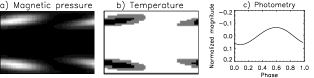
Figure 1: From the model calculations to the photometric observations. a) The magnetic pressure on the surface obtained from the model calculations. The brightest areas correspond to the largest magnetic pressure. b) The temperature map showing the spot configuration corresponding to the magnetic pressure distribution. In the map the black area has a temperature of 3500 K, grey corresponds to the temperature of 4250 K and white is the unspotted surface with the temperature of 5000 K. c) The normalised synthetic light-curve corresponding to the temperature map.

4 Results

The results from the thick and thin convection zone flip-flop models, that were first discussed in Elstner & Korhonen (elstner (2005)), have been converted into light-curves as described in the previous section. The model parameters are given in Table 2.

Table 2: The parameters for the models investigated in this paper. Table gives the name used for the model in the text, location of the inner boundary, the strength of the differential rotation (for solar differential rotation $\Omega_{0}=1$), dynamo-number $C_{\alpha}$ (Eq. 3), the energy density in equipartition units E0 for the component $m=0$ and E1 for $m=1$, the period of the oscillation in diffusion times and the migration period, also in diffusion times.

name	$r_{\rm in}$	$\Omega_{0}$	$C_{\alpha}$	E0	E1	P0	P1
thick	0.4	0.12	10	0.06	0.06	0.3	0.2
thin	0.7	0.11	21	0.1	0.4	0.23	0.46

In Fig. 2 an example of a sequence of temperature maps exhibiting a migrating spot pattern and a flip-flop event is shown. The features are symmetric with respect to the equator. It is clearly seen that in this thick convection zone model the spot shift in the flip-flop is $\sim 90^{\circ}$ and not 180°, as is more commonly seen in the observations.

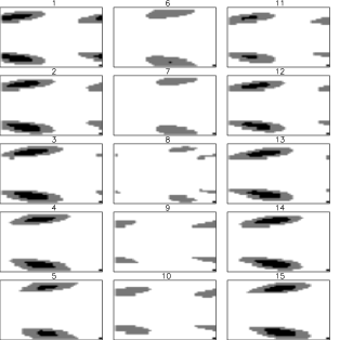
Figure 2: Temperature maps in a cylindrical projection showing a migrating spot pattern and a flip-flop event for the thick model. The colour coding is the same as in Fig. 1b. Each maps has 500 time steps in between them. Note that the small spot in the lower right corner is for enabling the correct plotting of the colours.

For investigating the long-term photometric behaviour obtained from the models, calculations were done starting around 80 diffusion times, running 50000 timesteps (one timestep is $1.9\cdot 10^{-5}$ diffusion times or approximately 1/5 days for our models) and calculating a map of magnetic pressure at the surface every 100 steps. These maps were then converted into temperature maps and synthetic light-curves, and the light-curves were plotted against time to see the long-term behaviour. Figs. 3a & b show the calculated light-curve behaviour for three different inclination angles for the thick and thin models, respectively.

Figure 3: The normalised magnitudes, calculated from the thick (a) and thin (b) convection zone flip-flop models, plotted against the timestep in the model for three different inclination angles. The series consists of synthetic light-curves calculated from 500 surface maps with 100 timesteps in between each map. The length of the whole series is thus slightly longer than 10 000 days ($\sim$28 years). The starting time for the series is around 80 convective turn-over times. The magnitudes have been normalised to the mean magnitude of the whole set.

In the case of the thick model (Fig. 3a) we see that the minimum magnitude is very strongly modulated during the flip-flop cycle, whereas the maximum magnitude is much less affected, except when viewed from small inclinations. The minimum and maximum in the maximum magnitude occur around the time of the minimum and maximum in the minimum magnitude. This behaviour is the same as seen by Fluri & Berdyugina (flu_ber (2004)) in their first case (sign-change of the axisymmetric component). The inclination of the star affects mainly the amplitude of the variation, as it determines how close the spots are to the centre of the visible disk (location of the maximum effect on the light-curve). In the case of high-latitude spots, as seen in these models, this effect totally dominates over the other inclination effect, i.e. how much of the spots on the “southern” hemisphere are visible. The changes in the inclination affect the behaviour of the maximum magnitude more strongly than the minimum magnitude.

The behaviour seen in the thin convection zone model (Fig. 3b) is different from the one seen in the thick model. The amplitude of the variation is much smaller because the active longitudes are further apart than in the thick case. It is also worth noting, that in this case the variation in the maximum and minimum magnitudes is very different from the thick case; here the maximum of the maximum magnitude occurs near the minimum of the minimum magnitude. There is a small shift towards the later timesteps for the maximum of the maximum magnitude in comparison to the minimum of the minimum magnitude.

5 Discussion

5.1 Dependence of the solution on the model parameters

The differential rotation needed for a flip-flop solution with a period of about 5 years is rather small. For a solar sized star the latitudinal difference in $\Omega$ ($\Delta\Omega$) should be about 10% of the solar value, independent of the global rotation. For $R_{\ast}=2R_{\odot}$ the $\Delta\Omega$ can be about 40%. The situation seems similar in all cases, i.e. for isotropic $\alpha$ tensor used together with a differential rotation depending on the distance to the rotation axis and with an anisotropic $\alpha$ tensor used with both a solar-like rotation law and axis distance dependent rotation law. An example of the time evolution of the magnetic field energy in the m=0,1 components with isotropic $\alpha$, $\Delta\Omega$ 30% of the solar value, and a rotation law depending on the axis distance (cf. Moss 2005) is shown in Fig. 4. As can be seen, with relatively strong differential rotation the non-axisymmetric component, m=1, is initially excited, but the mixed component solution survives only approximately 5 diffusion times.

Figure 4: Magnetic energy in axisymmetric (m=0) and non-axisymmetric (m=1) components for a model with $r_{c}=0.3$ and isotropic $\alpha$. The pole to equator difference of $\Omega$ is 30% of the solar value. The mixed component flip-flop solution survives only 5 diffusion times.

Increasing the diffusivity gives a strong flip-flop phenomenon also for higher pole to equator differences of $\Omega$, but with a smaller flip-flop period. The flip-flop solutions appear preferential for a positive $\alpha$ in the northern hemisphere in the case of radially increasing $\Omega$ at the equator. This leads to a poleward migration of the spots. Observations indicate solar-like equatorward migration pattern in solar-like stars (see e.g. Katsova et al. kats (2003)), but there is also a detection of poleward migration of the spots in the RS CVn binary HR 1099 (Vogt et al. vogt (1999); Strassmeier & Bartus str_bar (2000)).

5.2 Comparing the synthetic light-curves with the observations

Many active stars show long-term light-curves where time periods with small and large amplitude in the photometry alternate, as seen in our flip-flop models. For the behaviour seen in the thick model (Fig. 3a) a good stellar counterpart is DX Leo (see e.g. Messina & Guinan mes (2002)). It is easier to find stellar counterparts for the thin case (Fig. 3b). Some examples, like LQ Hya and EI Eri, can be seen for instance in Oláh & Strassmeier (olah_str (2002)). The fact that the thin case seems to be dominant implies that the flip-flops where the spots shift 180° are more common.

As seen in the case of FK Com (Oláh et al olah (2005)), some stars can show both 90° and 180° shifts in the spots during a flip-flop event. For investigating what alternating 90° and 180°  flip-flops would look like in the long-term photometry, we combine the calculated light-curves from the models showing 90° (from the thick model) and 180° (from the thin model) flip-flops, taking alternatively one 90° flip-flop and one 180° flip-flop. The result of combining the two types of flip-flops is shown in Fig. 5a. The long-term light-curve behaviour produced by this is similar, but not identical, to the second case of Fluri & Berdyugina (flu_ber (2004)), which shows alternatively small and large amplitude changes that are symmetric with respect to the mean magnitude, i.e. the maximum of the maximum magnitude occurs at the time of the minimum of the minimum magnitude. Our combination of the models with different spot shifts in the flip-flop event is symmetrical only during the smaller amplitude phase. During the larger amplitude phase the minimum of the maximum magnitude occurs at the time of the minimum of the minimum magnitude. For example, the light-curve of $\sigma$ Gem (see Fig. 5b) shows indications of this kind of behaviour.

Figure 5: a) The combination of the synthetic light-curves from the 90° and 180° flip-flops running approximately 9000 days, every other flip-flop is from different model. The 180° flip-flop calculations were moved slightly up for a more continuous plot. b) Light-curve of $\sigma$ Gem (from Henry et al. henry (1995)) shows indications of similar behaviour as seen in the panel a. Note the longer time span of the model (a) in comparison to the observations (b).

It is often difficult to see in the real observations the activity pattern caused by the flip-flop behaviour. This is partly due to the years long time series of observations needed to see the pattern and partly due to the solar-like cyclic changes in the over-all activity level of many active stars. Quite drastic changes in the brightness of some stars can be seen on top of the possible flip-flop signature (see e.g. HK Lac and IL Hya in Oláh & Strassmeier olah_str (2002)) and these large changes are likely to mask the patterns caused by the flip-flops.

6 Summary

We have synthesised photometry from Dynamo calculations exhibiting flip-flop behaviour. This was done for investigating the long-term changes in the photometric behaviour seen over several flip-flop cycles. On the whole, the activity patterns discussed in this paper imply flip-flop phenomenon and stars showing these patterns should be further investigated for checking if they really show flip-flops. A statistically significant sample of stars is needed for deeper understanding of this phenomenon. Further, more effort should be put to measuring the $\Delta\Omega$, meridional flow, and latitude migration of the spots on different types of stars. All these parameters have important implications for the dynamo calculations.

- (1) Al-Naimyi, H.M. 1978, ApSS, 53, 181
- (2) Berdyugina, S.V. 2004, Sol. Phys., 224, 123
- (3) Berdyugina, S.V., & Tuominen, I. 1998, A&A, 336, L25
- (4) Berdyugina, S.V., & Usoskin, I. 2003, A&A, 405, 1121
- (5) Berdyugina, S.V., Pelt, J., & Tuominen, I. 2002, A&A, 394, 505
- (6) Berdyugina S.V., Berdyugin A.V., Ilyin I., & Tuominen I. 1998, A&A, 340, 437
- (7) Elstner, D., & Korhonen, H. 2005, AN, 326, 278
- (8) Fluri, D., & Berdyugina, S.V. 2004, Sol. Phys., 224, 153
- (9) Henry G.W., Eaton J.A., Hamer J., & Hall D.S. 1995, ApJS, 97, 513
- (10) Järvinen, S.P., Berdyugina, S.V., Tuominen, I., & Strassmeier, K.G. 2005, A&A, 432, 657
- (11) Jetsu, L., Pelt, J., Tuominen, I., & Nations, H.L. 1991, in: The Sun and Cool Stars: activity, magnetism, dynamos, Tuominen I., Moss D., Rüdiger G. (eds.), Proc. IAU Coll. 130, Springer, Heidelberg, p. 381
- (12) Jetsu, L., Pelt, J., & Tuominen, I. 1993, A&A, 278, 449
- (13) Katsova, M.M., Livshits, M.A., & Belvedere, G. 2003, Sol. Phys., 216, 353
- (14) Korhonen, H., Berdyugina, S.V., Strassmeier, K.G., & Tuominen, I. 2001, A&A, 379, L30
- (15) Korhonen, H., Berdyugina, S.V., & Tuominen, I. 2002, A&A, 390, 179
- (16) Messina, S., & Guinan, E.F. 2002, A&A, 393, 225
- (17) Moss, D. 1999, MNRAS, 306, 300
- (18) Moss, D. 2004, MNRAS, 352, L17
- (19) Moss, D. 2005, A&A, 432, 249
- (20) Oláh, K., & Strassmeier, K. G. 2002, AN, 323, 361
- (21) Oláh, K., Korhonen, H., Kővari, Zs, Forgács-Dajka, E., & Strassmeier, K.G. 2005, A&A, submitted
- (22) Rodonò, M., Messina, S., Lanza, A.F., Cutispoto, G., & Teriaca, L. 2000, A&A, 358, 624
- (23) Strassmeier, K.G., & Bartus, J. 2000, A&A, 354, 537
- (24) Rüdiger, G., Elstner, D., & Ossendrijver, M. 2003, A&A, 406, 15
- (25) Vogt, S.S., Hatzes, A.P., Misch, A.A., & Kürster, M. 1999, ApJS, 121, 547