The fractal distribution of haloes

Abstract

We examine the proposal that a model of the large-scale matter distribution consisting of randomly placed haloes with power-law profile, as opposed to a fractal model, can account for the observed power-law galaxy-galaxy correlations. We conclude that such model, which can actually be considered as a degenerate multifractal model, is not realistic but suggests a new picture of multifractal models, namely, as sets of fractal distributions of haloes. We analyse, according to this picture, the properties of the matter distribution produced in cosmological $N$-body simulations, with affirmative results; namely, haloes of similar mass have a fractal distribution with a given dimension, which grows as the mass diminishes.

1 Introduction

The model of the large-scale matter distribution consisting of haloes with power-law profile and with centers distributed randomly can be traced back to Peebles [1]. McClelland & Silk [2] and later Sheth & Jain [3] and Murante et al [4] studied the effect on correlation functions of a spectrum of halo masses. The latter authors claimed that this model provides a good description of the observed galaxy correlations, at least on small scales. In particular, their analysis of generalized correlation integrals shows non-trivial scaling, which they consider indistinguishable from the scaling in fractal models. Recently, this conclusion has led Botaccio, Montuori and Pietronero [5] to construct new statistical functions to distinguish both types of models.

Motivated by the mentioned preceding works, here we critically examine the model of randomly distributed haloes with power-law profile. We instead propose a model consisting of a set of fractal distributions of haloes, that is, combining both the fractal and the halo models. Actually, Murante et al already considered to place the haloes “more deliberately, for instance in the sheet-like structures produced by large-scale pancake formation” but deferred it to future work. Here, we constructively proceed from the case of a single halo, understood as a degenerate multifractal model, to a general multifractal, considered as a set of fractal distributions of haloes. We argue that this model is plausible in regard to models of structure formation and provides a better description, especially, of void regions. Furthermore, we show that it is supported by the multifractal analysis of $N$-body simulations. We also discuss the rôle of the two-point correlation function in this context.

The halo model of large-scale structure, to be discussed further below, is now well developed [6]. Actually, clustering in the distribution of haloes has been studied by Mo & White [7] and Sheth & Tormen [8]. However, there is no study within the multifractal formalism yet (the paper by Murante et al [4] relates haloes with multifractals but is restricted to randomly distributed haloes). The advantage of this study is that it unveils the scaling properties and, in particular, allows us to deeply relate halo and fractal models.

2 Singularities and Multifractals

The standard magnitude used to describe fractals is the number-radius function $N(r)$, defined as the average number of points in a ball of radius $r$ centred on a point: it must be a power law, namely, $N(r)\sim r^{D}$, where $D$ is the fractal dimension. As a generalization of fractal distributions, multifractal measures represent mass distributions spread according to highly irregular patterns, so that a local density fails to exist. In fact, a multifractal measure is locally such that, in a ball of radius $r$ centred on a point $x$, $\mu[B({\mbox{\boldmath{$x$}}},r)]\sim r^{\alpha}$, where the Lipschitz-Hölder exponent $\alpha$ takes on a range of values [9]. For $\alpha<3$ the local density fails to exist, that is, there is no $\lim_{r\rightarrow 0}\mu[B({\mbox{\boldmath{$x$}}},r)]/r^{3}$ (it is divergent). On the other hand, for a differentiable distribution $\mu[B({\mbox{\boldmath{$x$}}},r)]\sim r^{3}$, so $\alpha=3$ and the density is $\rho({\mbox{\boldmath{$x$}}})=\lim_{r\rightarrow 0}\mu[B({\mbox{\boldmath{$x$}}},r)]/(\frac{4}{3}\pi r^{3})$.

Let us see how this definition applies to a differentiable distribution given by a single power law of the radius from a given point in space (placed at the origin), namely, $\rho(r)=A\,r^{-\beta},\>0<\beta<3$. This distribution is differentiable at every point except the origin, which is a singularity. Note that if ${\mbox{\boldmath{$x$}}}\neq 0$ then $\mu[B({\mbox{\boldmath{$x$}}},r)]\sim r^{3}$, whereas at the origin $\mu[B(0,r)]\sim r^{3-\beta}.$ The mass function $M(r)$, namely, the average of the mass in a ball of radius $r$ is

$$M(r)=\int d^{3}x\,\rho({\mbox{\boldmath{$x$}}})\,\mu[B({\mbox{\boldmath{$x$}}},r)]=\int d^{3}x\,{x}^{-\beta}\int_{B({\bf x},r)}d^{3}s\,{\left|{\mbox{\boldmath{$x$}}}+{\mbox{\boldmath{$s$}}}\right|}^{-\beta},$$ (1)

where we have to integrate over a finite region to have finite total mass (for example, with an $\left|{\mbox{\boldmath{$x$}}}\right|$ cutoff). This also renders $M(r)$ finite, for there is no divergence at ${\mbox{\boldmath{$x$}}}={\mbox{\boldmath{$s$}}}=0$. The function $M(r)$ can actually be computed in terms of trascendental functions, but this is not necessary, because only the behaviour of $M(r)$ in the limit of $r\rightarrow 0$ is needed. Therefore, in the integrand of Eq. (1) only two cases occur: either ${\mbox{\boldmath{$x$}}}\neq 0$ or ${\mbox{\boldmath{$x$}}}=0$ (the singularity). In the first case, the integral over $s$ in the $r\rightarrow 0$ limit yields ${x}^{-\beta}\,4\pi r^{3}/3\propto r^{3}$. In contrast, to calculate the integral at ${\mbox{\boldmath{$x$}}}=0$, we must perform the limit ${\mbox{\boldmath{$x$}}}\rightarrow 0$ before the limit $r\rightarrow 0$. The result is approximately $\int_{0}^{r}dx\,{x}^{2-\beta}\int_{0}^{r}ds\,{s}^{2-\beta}\propto r^{2(3-\beta)}$. Note that this quantity coincides with $\mu[B(0,r)]^{2}$. We conclude that if $\beta<3/2$ the behaviour of $M(r)$ in the limit of $r\rightarrow 0$ is $M(r)\propto r^{3}$ but if $\beta>3/2$ the behaviour is instead $M(r)\propto r^{2(3-\beta)}$ and is dominated by the singularity. An important remark is that, in the case dominated by the singularity, the value of the density $\rho({\mbox{\boldmath{$x$}}})$ at regular points (${\mbox{\boldmath{$x$}}}\neq 0$) is irrelevant and the result is therefore independent of its power-law form at those points.

We can consider a single power-law singularity as an example of multifractal [10]. In a generic multifractal the measure is concentrated in a set of vanishing Lebesgue measure, so that in almost every point there is no measure. The distribution of the measure is characterized by the multifractal spectrum, which can be calculated from the moment sums $M_{q}(r)=\sum_{\bf x}\mu[B({\mbox{\boldmath{$x$}}},r)]^{q}$ (generalized correlation integrals) [10, 9]. $M_{2}(r)$ is equivalent to $M(r)$ in Eq. (1). The larger the value of $q$, the more important is the contribution of the most singular points to the corresponding moment sum, and it can happen that only a few points (or a single one) contribute from some $q$ upwards. The multifractal spectrum $f(\alpha)$ is the function that gives the fractal dimension of the set of points with exponent $\alpha$, and can be calculated from the moments $M_{q}(r)$ ($r\rightarrow 0$).

For a distribution with one singularity with exponent $\alpha=3-\beta$ and regular with positive density everywhere else, the singularity contribution is $\mu[B(0,r)]^{q}\sim r^{q(3-\beta)}$ and the regular point contribution $\mu[B({\mbox{\boldmath{$x$}}},r)]^{q}\sim r^{3(q-1)}$. Therefore, if $q<3/\beta$ then $\alpha=f(\alpha)=3$ and if $q>3/\beta$ then $\alpha=3-\beta,\>f(\alpha)=0$. This degenerate multifractal spectrum can be derived in the standard way through the function $\tau(q)$ such that $M_{q}(r)\sim r^{\tau(q)}$. We have that $\tau(q)=3(q-1)$ if $q<3/\beta$ and $\tau(q)=q(3-\beta)$ if $q>3/\beta$, corresponding to $\alpha=3$ and $\alpha=3-\beta$, respectively. They yield the fractal dimensions of the singular set $f(\alpha=3)=\left.q\alpha-\tau(q)\right|_{\alpha=3}=3$ and $f(\alpha=3-\beta)=\left.q\alpha-\tau(q)\right|_{\alpha=3-\beta}=0$, respectively, as expected.

A generic multifractal is singular in an uncountable set of points (of vanishing Lebesgue measure). However, we can have intermediate cases, namely, distributions differentiable everywhere except in a set with “many” points and, furthermore, such that the measure is a power-law near every singular point. It is crucial what meaning we shall attribute to the word “many”. If the set of singularities is finite, then each one is isolated. If there is a common exponent, no novelties arise. Otherwise, depending on each singularity’s strength, as given by its exponent, $\tau(q)$ undergoes crossovers as $q$ increases, which can mimick a continuous variation. However, this type of multifractal is still degenerate and, in addition, $f(\alpha)$ jumps from 3 to 0 at once. All this applies to the model of randomly-placed power-law haloes [1, 2, 4].

Let us now consider the generalization to a distribution that is almost everywhere regular but with power-law singularities in a fractal set. Let us assume same strength singularities (common exponent $\alpha=3-\beta$, $0<\beta<3$) and everywhere non-vanishing density. A careless generalization of the case with a finite singularity set would make us believe that the multifractal spectrum is not altered and still $\tau(q)=3(q-1)$ if $q<3/\beta$ and $\tau(q)=q(3-\beta)$ if $q>3/\beta$ (corresponding to $\alpha=3$ and $\alpha=3-\beta$, respectively). However, this is now inconsistent, for it yields the fractal dimension of the singular set $f(\alpha=3-\beta)=\left.q\alpha-\tau(q)\right|_{\alpha=3-\beta}=0$, contrary to the assumption. So $\tau(q)\neq q(3-\beta)$ for $q>3/\beta$. In fact, given that $\alpha(q)=\tau^{\prime}(q)$, $\alpha$ constant only implies that $\tau(q)=\alpha\,q+c$, with $c$ being some arbitrary constant. Furthermore, $\tau(q)=\alpha\,q+c\Rightarrow f(\alpha)=-c$, so any dimension of the fractal singularity set $D=-c$ is allowed. Assuming $\tau(q)$ continuous, its change of behaviour takes place at $q=(3-D)/(3-\alpha)$, smaller than for a finite number of singularities of common strength (but larger than unity). The reason for the smaller value of $\tau(q)$ for $q>(3-D)/(3-\alpha)$ is that almost every point of a fractal is an accumulation point (because isolated points do not contribute to the fractal dimension), so the singularities are enhanced.

Summarizing, the generalization from a finite set of common strength singularities to a dimension-$D$ fractal set of common strength singularities leads to a crossover at smaller $q$ ($q\geq 1$) and with smaller (more singular) $\tau(q)=\alpha\,q-D$. A crossover between just two exponents $\alpha$ (one of which may be the trivial $\alpha=3$ or not) corresponds to a bifractal. Arguments for bifractal distributions of matter in cosmology have been given by Balian and Schaeffer [11], and Borgani [12] has shown that these distributions can be derived from the generalized thermodynamical model.

We can have several values of the exponent $\alpha$, like in the case of a finite singularity set. Therefore, we can have several crossovers, defining a multifractal spectrum degenerate by pieces. Let us consider the definition $D(q)=\tau(q)/(q-1)$, and the entropy dimension $D(1)=\alpha=f(\alpha)$, which defines the set of the measure’s concentrate. A monofractal is most degenerate, in the sense that there is only one $\alpha$, such that $f(\alpha)=\alpha$, of course. There are less degenerate cases in which $\alpha(q)$ is constant by pieces. In them the measure’s concentrate still has $f(\alpha)=\alpha$, but the other fractal sets with constant $\alpha$ have $f(\alpha)<\alpha$. To probe these sets one has to measure moments with the appropriate $q$’s.

Of course, a multifractal spectrum degenerate by pieces approaches a non-degenerate one as the number of pieces grows and the exponent $\alpha(q)$ becomes continuous. Usual physical mechanisms that generate singularities produce this type of spectrum. For example, the set of singularities of a mass distribution may be determined by some random process, such as the maxima of fractional Brownian motion. Models of this type are relevant in the context of the halo model of large-scale structure.

3 The halo model of large-scale structure

The halo model of large-scale structure takes its inspiration from old ideas on gravitational clustering of matter and also from the analysis of $N$-body simulations [6]. It assumes that the dark matter is in the form of collapsed and virialized haloes with definite density profile. This profile is usually taken to have spherical symmetry around the halo centre (with small deviations), with a given radial profile. This radial profile can adopt several forms, the simplest one being a power law $\rho(r)\propto r^{-\beta}.$

Complementary to the profile is the distribution of halo centres. Of course, it is simpler to consider a finite number of well-separated randomly-distributed haloes, but the usual mechanisms for large-scale structure formation produce an infinite number, unless a lower cutoff is introduced. This lower cutoff may appear as a softening of the gravitational force or as a minimal mass (both are present in $N$-body simulations). A lower cutoff prevents infinite clustering on small scales but nonetheless preserves clustering on larger scales. Let us focus on two models of large-scale structure formation, namely, the spherical collapse model and the adhesion model.

The spherical collapse model can be formulated in several ways; we here consider the formulation that takes the peaks of the initial Gaussian density field as seeds for the formation of haloes, so the number of haloes is directly determined by these peaks, although the spatial distribution and final halo masses depend on the ensuing dynamics. This nonlinear dynamics is complex but nonetheless enhances clustering. In any event, the set of peaks of a Gaussian density field is dense, so the assumption of a finite number of haloes is clearly insufficient. Arguably, this dense set of points becomes a set of fractals under the nonlinear dynamics, but this model does not allow to conclude much more without further assumptions on that nonlinear dynamics.

The adhesion model [13] provides us with a concrete nonlinear equation and methods to study the evolution of an initial Gaussian density field [14]. Actually, the evidence suggests the development of a distribution with multifractal features. It consists of a self-similar distribution of caustics: pancakes, filaments and nodes. Unfortunately, this model only covers the early stages of structure formation, before the virialization of haloes, which are supposed to arise essentially from the caustic nodes. The resulting distribution is probably similar to what Murante et al [4] had in mind as singularities “placed more deliberately, for instance in the sheet-like structures produced by large-scale pancake formation”.

Since the theoretical models of large-scale structure formation are insufficient to fully determine the structure and distribution of haloes, we may turn to $N$-body simulations. In fact, a good deal of evidence for the halo model comes from them. However, discretization issues tend to make the conclusions less certain. For example, the inevitable smoothing length that is introduced in the gravitational interaction suppresses clustering on smaller scales, so that the smoothness of haloes may be just a consequence of it rather than a consequence of the gravitational dynamics. At any rate, the smoothness of haloes is questionable and there is evidence for a hierarchical structure of condensations, similar to a multifractal [15].

Multifractal analyses of large-scale structure were first introduced regarding the distribution of galaxies [16, 17] and later applied to $N$-body simulations [18, 19, 20], with positive results. However, the relationship of these results with haloes and their distribution is far from clear. One way to clarify this relationship is to give a definition of haloes suitable for $N$-body simulations and then analyse their spatial distribution. In a multifractal model, haloes must be identified with density singularities, but there are no real singularities in $N$-body simulations. One can define a coarse-grained density and consider density peaks as singularities, in accord with coarse multifractal analysis [9]. Then one can measure the strength of singularities and analyse the distributions of singularities of similar strength, to assess their fractality. This is an alternative (or rather complementary) procedure to the computation of moments and hence the multifractal spectrum $f(\alpha)$.

We have applied this new picture of multifractal models to $N$-body cosmological simulations by the Virgo Consortium; in particular, we have taken the $z=0$ positions of the $\Lambda$CDM GIF2 simulation, with $400^{3}$ particles in a volume of (110 $h^{-1}$ Mpc)³ [21]. To measure the strength of singularities, we use a spatial window, for several window lengths. To simplify matters, we select two different singularity strengths, corresponding to two different halo masses (at definite window length); hence we classify the haloes in heavy and light haloes, in a sort of bifractal. If we were to identify haloes as the places of galaxy formation, this selection would roughly correspond to two types of galaxies that have been used in connection with voids in the galaxy distribution, namely, “wall” and “field” galaxies. Results of an analysis with window length $r=2^{-8}$ appear in Fig. 1: On the left-hand side, there is a slice showing both halo populations, consisting of 2508 and 25556 members, with 750 to 1000 particles and with 100 to 150 particles, respectively. On the right-hand side, we have log-log plots of the number-radius functions for the respective spatial distributions of halo centers. They have scaling ranges corresponding to quite different fractal dimensions, namely, $D_{1}=1.1$ and $D_{2}=1.9$. We have also carried out the analysis of moments and derived the multifractal spectrum. It yields entropy dimension $D(1)=2.5$ and shows that the values of the fractal dimensions $f(\alpha_{1})=1.1$ and $f(\alpha_{2})=1.9$ in Fig. 1 correspond (approximately) to $\alpha_{1}=1.5$ and $\alpha_{2}=2.0$, and to $q_{1}=2.3$ and $q_{2}=1.5$. These noninteger values are relatively close to the integer $q=2$, associated with the two-point correlation function. The role of the various $M_{q}$ and, in particular, of $M_{2}$ is further discussed below.

We can observe that the light haloes are somewhat clustered, as corresponds to a fractal of dimension $\simeq 2$. In fact, more uniform distributions can be found for even lighter haloes, and the most uniform distribution corresponds to the largest fractal dimension, namely, $D(0)$. The estimation of $D(0)$ is affected by the problem of undersampling, especially for small window length. However, it seems that $D(0)=3$ is already reached for values of the window length $r=2^{-7}\simeq 0.01$, that is, well within the scaling range. Indeed, in the scale range $2^{-7}$–$2^{-4}$ we have a stable multifractal spectrum. Note that these scales correspond to physical length $\simeq 1$–$7\;h^{-1}$ Mpc, larger than the size of virialized haloes.

We remark that $\alpha(q=0)\simeq 3.3>3$, such that the distribution at the corresponding points is regular with vanishing density. So there are no haloes at those points, which actually belong to voids. The set of regular points with non-vanishing density corresponds to $\alpha=3$ and $f(\alpha)\simeq 2.9$, which is nearly homogeneous.

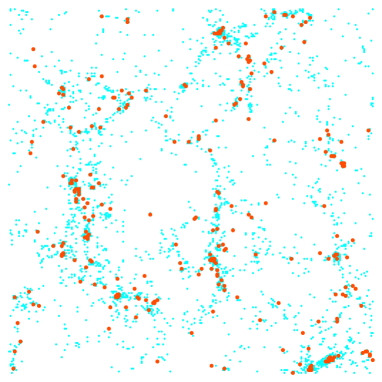
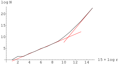
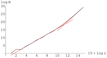
Figure 1: Selection of two halo populations from the GIF2 $N$-body simulation: heavy haloes with 750 to 1000 particles and light haloes with 100 to 150 particles. (Left) Slice showing heavy haloes in red and light haloes in blue. (Right) Number-radius function for the heavy haloes (above) and the light haloes (below), showing fractal dimensions $D=1.1$ and $D=1.9$, respectively, and a transition to homogeneity in both (logarithms are to base $\sqrt{2}$ and the total size is normalized to unity).

4 Conclusions

We have seen, in a model of the large-scale matter distribution consisting of randomly placed haloes with power-law profile, that the power-law form of correlation functions as $r\rightarrow 0$ is due to the singularities of the power-law distribution, rather than to its regular part. We have also seen that it is only a particular and degenerate case of a multifractal distribution. While a suitable spectrum of singularity strengths can reproduce the scalings observed in the galaxy distribution [4], underdense regions are necessarily homogenous and there are no voids. Therefore, we consider the generalization to a multifractal model consisting of a set of fractal distributions of power-law haloes. A degenerate model with a set of discrete singularity strengths is useful conceptually and to analyse $N$-body simulations. We have analysed in the GIF2 simulation the distributions of singularities with several strengths. They show well-defined scaling ranges, with different scaling dimension, and their transition to homogeneity. We have selected two representative populations of heavy or light haloes, with fractal dimensions $D=1.1$ and $D=1.9$. We remark that these two values span the usual range of fractal dimensions of the galaxy distribution.

As to the rôle of the two-point correlation, it is certainly not sufficient to fully characterize the scaling properties of the dark matter distribution and one has to study higher order correlations. This is characteristic of multifractals, which are defined by the full set of moments $M_{q}(r)$ for $-\infty<q<\infty$, as opposed to pure fractals, defined only by $M_{2}(r)$ (in fact, by $M_{q}\sim M_{2}^{q-1}$, with any $q$). In addition, we remark that the singular nature of multifractals implies that the moments with $q=2,3,\ldots$ are not sufficient. The restriction to these moments amounts to considering a multifractal degenerate by pieces, but with an inadequate division. In fact, most important is $q\simeq 1$, because the entropy dimension $D(1)=\alpha=f(\alpha)$ defines the set of the measure’s concentrate. Larger $q$’s are also relevant but very little information is actually gathered from moments with $q>6$ (in current $N$-body simulations). Negative-$q$ moments are relevant as well, but not in connection with haloes but with voids. At any rate, if we focus on a uniform set of haloes, namely, on a definite set of singularities with similar strength, the two-point correlation function of their centers provides the necessary information for its scaling properties. Since this is true for every set of singularities, the corresponding set of two-point correlation functions defines the scaling properties of the full distribution. Precisely this is the basis of the picture of the full distribution as a set of fractal distributions of haloes that we propose.

5 Acknowledgments

I am grateful to Liang Gao for kindly supplying me with the GIF2 data and to Marco Montuori for correspondence regarding their paper [5]. My work is supported by the “Ramón y Cajal” program and by grant BFM2002-01014 of the Ministerio de Educación y Ciencia.

References

- [1] \NamePeebles, P.J.E. \REVIEWA&A321974197
- [2] \NameMcClelland, J. Silk, J. \REVIEWApJ2171977331
- [3] \NameSheth, R.K. & Jain, B. \REVIEWMNRAS2851997231
- [4] \NameMurante, G., Provenzale, A., Spiegel, E.A., Thieberger, R. \REVIEWMNRAS2911997585
- [5] \NameBotaccio, M., Montuori M., Pietronero, L. \REVIEWEurophysics Letters662004610
- [6] \NameCooray, A. & Sheth, R. \REVIEWPhys. Rep.37220021
- [7] \NameMo, H.J. & White, S.D.M. \REVIEWMNRAS2821996347
- [8] \NameSheth, R.K. & Tormen, G. \REVIEWMNRAS3081999119
- [9] \NameFalconer, K. \BookFractal geometry \PublJohn Wiley & Sons, Chichester, UK \Year2003
- [10] \NameHalsey, T.C., Jensen, M.H., Kadanoff, L.P., Procaccia, I. & Shraiman, B.I. \REVIEWPhysical Review A3319861141
- [11] \NameBalian, R. Schaeffer, R. \REVIEWA&A2261989373
- [12] \NameBorgani, S. \REVIEWMNRAS2601993537
- [13] \NameGurbatov, S.N., Saichev, A.I. & Shandarin, S. \REVIEWMNRAS2361989385
- [14] \NameVergassola, M., Dubrulle, B., Frisch, U. & Noullez, A. \REVIEWA&A2891994325
- [15] \NameValageas, P. \REVIEWA&A3471999757
- [16] \NameDomínguez-Tenreiro, R., & Martínez, V.J. \REVIEWApJ3391989L9
- [17] \NameMartínez, V.J., Jones, B.J., Domínguez-Tenreiro, R. & van de Weygaert, R. \REVIEWApJ357199050
- [18] \NameColombi, S., Bouchet, F.R. Schaeffer, R. \REVIEWA&A26319921;
- [19] \NameValdarnini, R., Borgani, S. Provenzale, A. \REVIEWApJ3941992422;
- [20] \NameYepes, G., Dominguez-Tenreiro, R. Couchman, H.P.M. \REVIEWApJ401199240;
- [21] \NameGao, L., White, S.D.M., Jenkins, A., Stoehr, F. & Springel, V. \REVIEWMNRAS3552004819