Measuring the cosmic evolution of dark energy with baryonic oscillations in the galaxy power spectrum

Abstract

We use Monte Carlo techniques to simulate the ability of future large high-redshift galaxy surveys to measure the temporal evolution of the dark energy equation-of-state $w(z)$, using the baryonic acoustic oscillations in the clustering power spectrum as a ‘standard ruler’. Our analysis only utilizes the oscillatory component of the power spectrum and not its overall shape, which is potentially susceptible to broadband tilts induced by a host of model-dependent systematic effects. Our results are therefore robust and conservative. We show that baryon oscillation constraints can be thought of, to high accuracy, as a direct probe of the distance — redshift and expansion rate — redshift relations where distances are measured in units of the sound horizon. Distance precisions of 1% are obtainable for a fiducial redshift survey covering $10{,}000$ deg² and redshift range $0.5<z<3.5$. If the dark energy is further characterized by $w(z)=w_{0}+w_{1}z$ (with a cut-off in the evolving term at $z=2$), we can then measure the parameters $w_{0}$ and $w_{1}$ with a precision exceeding current knowledge by a factor of ten: $1\sigma$ accuracies $\Delta w_{0}\approx 0.03$ and $\Delta w_{1}\approx 0.06$ are obtainable (assuming a flat universe and that the other cosmological parameters $\Omega_{\rm m}$ and $h$ could be measured independently to a precision of $\pm 0.01$ by combinations of future CMB and other experiments). We quantify how this performance degrades with redshift/areal coverage and knowledge of $\Omega_{\rm m}$ and $h$, and discuss realistic observational prospects for such large-scale spectroscopic redshift surveys, with a variety of diverse techniques. We also quantify how large photometric redshift imaging surveys could be utilized to produce measurements of $(w_{0},w_{1})$ with the baryonic oscillation method which may be competitive in the short term.

1 Introduction

In the current standard cosmological model, baryonic matter and cold dark matter together contribute only about a third of the total energy density of the Universe. One of the most important puzzles in cosmology is to account for the remaining two-thirds of the energy, which is required to render the Universe approximately spatially flat, as demanded by recent observations of the Cosmic Microwave Background (CMB; de Bernardis et al., 2000).

The existing set of cosmological data – consisting principally of measurements of the CMB, of the local clustering of galaxies, and of distant supernovae – can be understood by invoking the existence of the ‘cosmological constant’ $\Lambda$ originally envisaged by Einstein, such that it contributes a present-day fractional energy density $\Omega_{\Lambda}=0.73\pm 0.04$ (Spergel et al., 2003). The remarkable consequence of this model is that $\Lambda$ acts as a ‘repulsive gravity’, driving the rate of cosmic expansion into a phase of acceleration. Equally surprisingly, this acceleration has been observed reasonably directly by an apparent dimming of distant supernovae (Riess et al., 1998; Perlmutter et al., 1999).

The cosmological constant component is naturally attributed to the inherent energy density of the vacuum. However, the ‘expected’ quantum-mechanical Planck energy density is larger than that required to account for the accelerating rate of cosmic expansion by an exceptionally large dimensionless factor of order $c^{5}\,G^{-1}\hbar^{-1}H_{0}^{-2}$ $\sim 10^{122}$. This profound difficulty has motivated the development of alternative models for the ‘dark energy’ – i.e. the causative agent of accelerating expansion. Many of these models, such as ‘quintessence’ (Ratra & Peebles, 1988), feature a dynamic component of dark energy whose properties evolve with time (e.g. a rolling scalar field $\phi$). These predictions are commonly characterized in terms of the dark energy equation-of-state $w(z)=P/\rho$, relating its pressure $P$ to its energy density $\rho$ (in units where the speed-of-light $c=1$). For the cosmological constant model, $w(z)=-1$ at all epochs.

These competing models for the dark energy are essentially untested, because the current cosmological dataset is not adequate for delineating variations in the function $w(z)$ with redshift, which is the essential requirement for distinguishing quintessential cosmologies from a cosmological constant. New experiments are demanded, which must be able to recover the characteristics of dark energy with unprecedented precision, including any cosmic evolution. The study of the nature of dark energy is the current frontier of observational cosmology, and has been widely identified as having profound importance for physics as a whole (Turner et al., 2003).

Given the fundamental importance of accelerating cosmic expansion and the possibility of confounding systematic effects in the supernova data, other precision probes of the dark energy model are clearly desirable. In Blake & Glazebrook (2003), hereafter Paper I, we suggested that the small-amplitude ‘baryonic oscillations’, which should be present in the power spectrum of the galaxy distribution on large scales ($\gtrsim 30$ Mpc), could be used as a ‘standard cosmological ruler’ to measure the properties of dark energy as a function of cosmic epoch, provided that a sufficiently-large high-redshift ($z\gtrsim 1$) galaxy survey was available (see also Seo & Eisenstein, 2003; Linder, 2003; Hu & Haiman, 2003). The characteristic sinusoidal ruler scale encoded by the baryonic oscillations is the sound horizon at recombination, denoted $s$. This length scale is set by straight-forward linear physics in the early Universe and its value is determined principally by the physical matter density ($\rho_{m}\propto\Omega_{m}h^{2}$). The cosmological uncertainty in this parameter combination is ameliorated by an advantageous cancellation of pre-factors of $\Omega_{m}h^{2}$ in the ratio of low-redshift distances to $s$ (see Paper I). The residual dependence of $s$ on $\Omega_{m}$ and other cosmological parameters is small (Eisenstein & White, 2004), rendering observations of the acoustic oscillations a powerful geometric probe of the cosmological model.

This acoustic signature has recently been identified at low redshift in the distribution of Luminous Red Galaxies in the Sloan Digital Sky Survey (Eisenstein et al., 2005) (see also Cole et al., 2005). Although these data are insufficient for precise measurements of the dark energy, this analysis represents a striking validation of the technique. The challenge now is to create larger and deeper surveys. In Paper I we demonstrated that, given a galaxy redshift survey at $z\sim 1$ mapping a total cosmic volume several times greater than that of the Sloan main spectroscopic survey in the local Universe (we define $V_{\rm Sloan}\equiv 2\times 10^{8}\,h^{-3}$ Mpc³), the equation-of-state of the dark energy could be recovered to a precision $\Delta w\approx 0.1$ (assuming a model in which $w$ is constant). The precision of this experiment scales with cosmic volume $V$ in a predictable manner (roughly in accordance with $1/\sqrt{V}$) and it is not unfeasible to imagine an ultimate ‘all-sky’ high-redshift spectroscopic survey within $\sim 20$ years.

We believe that this standard ruler technique would powerfully complement proposed future supernova searches such as the SNAP project (e.g. Aldering et al., 2002, http://snap.lbl.gov) permitting, for example, direct tests of the ‘reciprocity relation’ which predicts that the true luminosity distance $d_{L}(z)$ (measured by a standard candle) is exactly the same as the angular diameter distance $d_{A}(z)$ (measured by a standard ruler), up to a factor of $(1+z)^{2}$ (Bassett & Kunz, 2004). Furthermore, we argue that it is not yet conclusively proven that the dimming of supernovae caused by cosmic acceleration can be distinguished with sufficient accuracy from other possible systematic effects, such as changes in the intrinsic properties of supernovae with galactic environment (e.g. metallicity), dust extinction effects, population drift and the difficulties of sub-percent-level photometric calibration (including K-corrections) across wide wavelength ranges. It is therefore important to pursue alternative precise high-redshift probes of the cosmological model. A particular advantage of the baryonic oscillations method is that it is probably free of major systematic errors, assuming that galaxy biasing on large scales is not pathological.

In Paper I we developed a Monte Carlo, semi-empirical approach to transforming synthetic galaxy redshift surveys into constraints on the value of $w$. This contrasts with, and complements, other analytical approaches to the problem such as those using Fisher-Information techniques (e.g. Seo & Eisenstein, 2003; Hu & Haiman, 2003). In this present study we extend and refine our methodology to the more general case where we allow the equation-of-state of dark energy to have a dependence on redshift, $w(z)=w_{0}+w_{1}z$, and we recover joint constraints upon $(w_{0},w_{1})$. Furthermore, we apply the standard ruler independently to the radial and tangential components of the power spectrum, which has the effect of producing separate measurements of the co-moving angular-diameter distance to the effective redshift of each survey slice, $x(z)$, and the rate of change of this quantity with redshift, $x^{\prime}(z)\equiv dx/dz$. We note for clarity that in a flat Universe:

$$x(z)=D_{A}(z)(1+z)$$

$$x^{\prime}(z)=c/H(z)$$

where $D_{A}$ is the physical angular diameter distance and $H(z)$ is the Hubble factor (Universal expansion rate) at redshift $z$. We also examine in more detail the effect of uncertainties in cosmological parameters such as the matter density and the Hubble parameter. In addition, we present an in-depth discussion of the observational requirements and prospects for realistic surveys, based upon both spectroscopic redshifts and photometric redshifts.

The plan of this paper is as follows: in Section 2 we give a very detailed description of our methodology, greatly expanding on Paper I, and the approximations we made to allow us to simulate a range of large surveys, and in Section 3 we quantify the size of redshift survey required to detect the oscillatory component of the power spectrum. The recovered constraints on $(w_{0},w_{1})$ for various simulated surveys are presented in Section 4 for spectroscopic surveys and in Section 5 for photometric-redshift surveys. Finally, in an Appendix we present the results of a very large computation designed to test the effects of our approximations.

2 Monte Carlo Methodology

Our methodology for simulating future galaxy redshift surveys and assessing their efficacy for measuring acoustic oscillations was summarized in Paper I. In this Section we provide a more detailed account of our procedures. In addition, we have implemented various extensions to the methodology of Paper I:

1. We now fit separate acoustic oscillation scales in the tangential and radial directions. In Paper I we fitted to the angle-averaged power spectrum, effectively assuming that the shift in the apparent radial and transverse scales as the cosmology was perturbed about the fiducial value were the same. This is only approximately true for $z\sim 1$ and breaks down at low and high redshift (see Figure 5 of Paper I). In the new approach we make use of the different redshift dependencies of radial and transverse scales to provide extra cosmological constraints increasing signal:noise. Specifically, the tangential scale is controlled by the co-moving distance to the effective redshift of the survey, $x(z)$, and the radial scale is determined by the rate of change of this quantity with redshift, $x^{\prime}(z)\equiv dx/dz=c/H(z)$, where $H(z)$ is the Hubble constant measured by an observer at redshift $z$. This is useful because $H(z)$ is directly sensitive to the dark energy density at the redshift in question.

2. We allow the equation-of-state of dark energy $w(z)$ to have a dependence on redshift, $w(z)=w_{0}+w_{1}z$, and we recover joint constraints upon $(w_{0},w_{1})$. We do not claim that this expression faithfully describes dark energy in the real Universe. In particular, models with $w_{1}>0$ become unphysical at high redshift unless we impose a cut-off for the evolving term: we assume that $w(z>z_{\rm cut})=w_{0}+w_{1}z_{\rm cut}$ where $z_{\rm cut}=2$, and we ensure that matter dominates at high redshift, i.e. $w_{1}\leq(-w_{0})/z_{\rm cut}$. However, usage of the equation $w(z)=w_{0}+w_{1}z$ facilitates comparison with other work such as Seo & Eisenstein (2003) who use the same parameterization, empirically describes a range of dark energy models (Weller & Albrecht, 2002), and permits a first disproof of the cosmological constant scenario, if $w_{1}\neq 0$ and/or $w_{0}\neq-1$. We note that the alternative parameterization $w(z)=w_{0}+w_{a}(1-a)$, where $a=(1+z)^{-1}$ is the usual cosmological scale factor, encodes a more physically reasonable behaviour at high redshift (Linder, 2002). In this paper we compute $(w_{0},w_{a})$ constraints for one case.

3. We place Gaussian priors upon the other relevant cosmological parameters, the matter density $\Omega_{\rm m}$ and the Hubble parameter $h=H(z=0)/(100$ km s^-1 Mpc${}^{-1})$, rather than assuming that their values are known precisely.

2.1 Method Summary

As described in Paper I, the philosophy of our analysis is to maintain maximum independence from models. When measuring the acoustic oscillations from simulated data, we divide out the overall shape of the power spectrum via a smooth ‘reference spectrum’. We then fit a simple empirically-motivated decaying sinusoid to the remaining oscillatory signal. Hence we do not utilize any information encoded by the shape of the power spectrum. This shape may be subject to smooth broad-band systematic tilts induced by such effects as complex galaxy biasing schemes, quasi-linear growth of structure, a running primordial spectral index, and redshift-space distortions. However, it would be very surprising if any of these phenomena introduced oscillatory features in $k$-space liable to obscure the distinctive acoustic peaks and troughs. We note that any model where the probability of a galaxy forming depends only on the local density field leads to linear bias on large scales (Coles, 1993; Scherrer & Weinberg, 1998). Furthermore, linear biassing is observed to be a very good approximation on large scales (e.g. Peacock & Dodds, 1994; Cole et al., 2005). This is in agreement with numerical simulations of galaxy formation which show that galaxies and/or massive haloes faithfully reproduce the acoustic oscillations (Springel et al., 2005; Angulo et al., 2005).

Of course, a full power spectrum template should be fitted to real data as well: our aim here is to derive robust, conservative lower limits to the efficacy of baryon oscillations experiments, using only the information contained in the oscillations.

An important point is that the fractional error in the measured galaxy power spectrum, $\sigma_{P}/P$, after division by a smooth overall fit, is independent of the absolute value of $P(k)$ if the error budget is dominated by cosmic variance rather than by shot noise. In this sense, an incorrect choice of the underlying model power spectrum in our simulations does not seriously affect the results presented here. Having secured a detection of the acoustic signature, if one is then prepared to model the underlying power spectrum – correcting for such systematic effects as non-linear gravitational collapse, redshift-space distortions and halo bias – then more accurate constraints on cosmological parameters would follow (see Eisenstein et al., 2005).

In summary (see Section 2.2 for a more detailed account): we generate a model matter power spectrum in the linear regime using the fitting formulae of Eisenstein & Hu (1998), assuming a primordial spectral index $n=1$ (as suggested by inflationary models) and fiducial cosmological parameters $\Omega_{\rm m}=0.3$, $h=0.7$ and baryon fraction $\Omega_{\rm b}/\Omega_{\rm m}=0.15$, broadly consistent with the latest determinations (e.g. Spergel et al., 2003). In Paper I we showed that the cosmological constraints are fairly insensitive to the exact value of $\Omega_{\rm b}/\Omega_{\rm m}$ (Figures 7–8 in Paper I; increasing $\Omega_{\rm b}$ results in a somewhat higher baryonic oscillation amplitude, hence a more precise measure of the standard ruler). We assume that the shape of $P(k)$ does not depend on the dark energy component, and take the $z=0$ normalization $\sigma_{8}=1$. The model $P(k)$ is then used to generate Monte Carlo realizations of a galaxy survey covering a given geometry, deriving redshifts and angular co-ordinates for the galaxies using a fiducial flat cosmological constant model. The realizations are then analyzed for a grid of assumed dark energy models. $P(k)$ is measured using a Fast Fourier Transform (FFT) up to a maximum value of $k$ determined by a conservative estimate of the extent of the linear regime at the redshift in question (see Paper I, Figure 1). The measured power spectrum is fitted with a decaying sinusoid with the ‘wavelength’ as a free parameter. By comparing the fiducial wavescale (determined using the values of $\Omega_{\rm m}h^{2}$ and $\Omega_{\rm b}h^{2}$ in conjunction with a standard fitting formula, e.g. Efstathiou & Bond (1999)) with the distribution of fitted wavescales across the Monte Carlo realizations, we can reject each assumed dark energy model with a derivable level of significance. We assume a flat universe (in Section 2.4, Figure 6 below we indicate how our dark energy measurements weaken with declining knowledge of $\Omega_{\rm k}$).

Throughout this paper we ensure that our model galaxy surveys contain sufficient objects that the contribution of shot noise to the error in the power spectrum is sub-dominant to that of cosmic variance. In an analytical treatment (e.g. Tegmark, 1997), the relative contributions of shot noise and cosmic variance can be conveniently expressed in terms of the quantity $n\times P$, where $n$ is the typical number density of galaxies in the survey volume and $P$ is the galaxy power spectrum evaluated at some typical scale measured by the survey. Analytically, the errors due to shot noise and to cosmic variance are equal when $n\times P=1$. For the simulations described in this paper, we uniformly populated the survey volume with sufficient galaxies that $n\times P=3$, where $P$ is evaluated at a characteristic scale $k=0.2\,h$ Mpc^-1. The surface density of galaxies required to achieve this condition is illustrated in Figure 1.

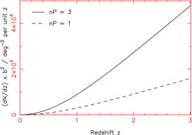
Figure 1: The surface density of galaxies per unit redshift, $dN/dz$, required to achieve power spectrum shot noise levels $n\times P=1$ (dashed line; equal error contribution due to shot noise and to cosmic variance) and $n\times P=3$ (solid line; adopted in our simulations). The power spectrum $P$ is evaluated at a ‘typical’ scale $k=0.2\,h$ Mpc^-1; at zero redshift this value is taken to be $P=2500\,h^{-3}$ Mpc³ (and is scaled to higher redshifts using the square of the linear growth factor $D_{1}(z)$). If the galaxies possess a linear bias $b$, then the amplitude of their power spectrum scales as $b^{2}$ and a proportionately lower surface density is required. For $b=1$ galaxies in a redshift slice of width $\Delta z=0.2$ at $z=1$, a density $\approx 1800$ deg^-2 is required to achieve $n\times P=3$.

2.2 Detailed fitting methodology

Here we outline the Monte-Carlo approach we have implemented in our code. In fact for most of our analysis we utilized a simple approximation as explained in Section 2.3: to be specific we omitted steps 8 and 9 below, which are very expensive in computational resources (we test this approximation in the Appendix).

1. A fiducial cosmology is chosen for the simulation: for example $(\Omega_{\rm m},h,w_{0},w_{1})=(0.3,0.7,-1,0)$. A fiducial baryon fraction is selected ($\Omega_{\rm b}/\Omega_{\rm m}=0.15$).

2. A survey redshift range $(z_{\rm min},z_{\rm max})$ and solid angle is specified: for example $1.0<z<1.3$ and $1000$ deg². The survey sky geometry is assumed to be bounded by lines of constant right ascension and declination of equal angular lengths. The three-dimensional geometry is therefore ‘conical’ and the convolving effect of this window function is included.

3. Using the fiducial cosmology, a cuboid for FFTs is constructed whose sides $(L_{x},L_{y},L_{z})$ are just sufficient to bound the survey volume. Note, only the enclosed cone is populated by galaxies in order that the window function effect is treated properly.

4. A model matter power spectrum $P_{\rm mass}(k,z=0)$ is computed for the chosen parameters $(\Omega_{\rm m},\Omega_{\rm b},h)$ from the fitting formula (Eisenstein & Hu, 1998), assuming a $z=0$ normalization $\sigma_{8}=1$ and a primordial power-law slope $n=1$. The survey slice is assumed to have an ‘effective’ redshift $z_{\rm eff}=(z_{\rm min}+z_{\rm max})/2$. The power spectrum is scaled to this redshift using the linear growth factor $D_{1}(z)$, obtained by solving the full second-order differential equation (see e.g. Linder & Jenkins, 2003) to enable us to treat non-$\Lambda$CDM cosmologies:

   $$P_{\rm gal}(k,z_{\rm eff})=P_{\rm mass}(k,0)\,D_{1}(z_{\rm eff})^{2}\,b^{2}$$ (1)

   where we use a constant linear bias factor $b$ for the clustering of galaxies with respect to matter. The value $b=1$ is assumed for our surveys, unless otherwise stated.

5. A set of Monte Carlo realizations (numbering 400 for all simulations presented here) is then performed to generate many different galaxy distributions consistent with $P_{\rm gal}(k)$, as described in steps 6 and 7.

6. A cuboid of Fourier coefficients is constructed with grid lines set by $dk_{i}=2\pi/L_{i}$, with a Gaussian distribution of amplitudes determined from $P_{\rm gal}(k)$, and with randomized phases. The gridding is sufficiently fine that the Nyquist frequencies in all directions are significantly greater than the smallest scale for which a power spectrum is extracted (i.e. the linear/non-linear transition scale at the redshift $z_{\rm eff}$).

7. The Fourier cuboid is FFTed to determine the density field in the real-space box. This density field is then Poisson sampled within the survey ‘cone’ to determine the number of galaxies in each grid cell.

8. Using the fiducial cosmological parameters, this distribution is converted into a simulated catalogue of galaxies with redshifts and angular positions, for each Monte Carlo realization.

9. We now assume a trial cosmology: for example $(\Omega_{\rm m},h,w_{0},w_{1})=(0.3,0.7,-0.9,0)$. The co-moving co-ordinates of the galaxies are computed in the trial cosmology as would be done by an observer without knowledge of the true cosmology.

10. The power spectrum of the simulated survey for the trial cosmology is measured using standard estimation tools (Feldman, Kaiser, & Peacock, 1994). Power spectrum modes in Fourier space are divided into bins of $(k_{\rm perp},k_{\rm par})$ where, if the $x$-axis is the radial direction, $k_{\rm par}=k_{x}$ and $k_{\rm perp}^{2}=k_{y}^{2}+k_{z}^{2}$.

11. An error bar is assigned to each power spectrum bin using the variance measured over the Monte Carlo realizations. Note that the distribution of realizations also encodes any covariances between different power spectrum bins, although the scale of correlations in $k$-space is expected to be very small (compared to the separation of the acoustic peaks) for the very large survey volumes considered here.

12. The measured $P(k_{\rm perp},k_{\rm par})$ is divided by a smooth ‘reference spectrum’ following Paper I (i.e. the ‘no-wiggles’ spectrum of Eisenstein & Hu, 1998), and the result is fitted with a simple empirical formula, modified from Paper I to permit separate fitting of the sinusoidal scale in the radial and tangential directions:

    $$\frac{P(k_{\rm perp},k_{\rm par})}{P_{\rm ref}}=1+$$ (2)

    $$A\,k\,\exp{\left[-\left(\frac{k}{0.1\,h\,{\rm Mpc}^{-1}}\right)^{1.4}\right]}\times$$

    $$\sin{\left(2\pi\sqrt{\left(\frac{k_{\rm perp}}{\lambda_{\rm perp}}\right)^{2}+\left(\frac{k_{\rm par}}{\lambda_{\rm par}}\right)^{2}}\right)}$$

    where $k^{2}=k_{\rm perp}^{2}+k_{\rm par}^{2}$. The free parameters are then the tangential and radial sinusoidal wavescales $(\lambda_{\rm perp},\lambda_{\rm par})$ together with the overall amplitude $A$.

We can now assign a probability to the trial cosmology. The Monte Carlo realizations produce a distribution of fitted wavescales $\lambda_{\rm perp}$ and $\lambda_{\rm par}$ (Figure 2) for the trial cosmology. Using these trial cosmological parameters, we can determine the length of the characteristic ruler $\lambda_{\rm theory}$ using a standard fitting formula for the sound horizon integral (Equation 1, Paper 1) in terms of $\Omega_{\rm m}$, $\Omega_{\rm b}$ and $h$ (Efstathiou & Bond, 1999). (We remind the reader that $\lambda_{\rm theory}$ is set in the early Universe and is insensitive to dark energy parameters.) The location of the value of $\lambda_{\rm theory}$ in the distribution of tangential (radial) wavescales over the Monte Carlo realizations allows us to assign a probability for the trial cosmological parameters. For example: if $\lambda_{\rm theory}$ lies at the $16^{\rm th}$ percentile of the distribution, the rejection probability is $2\times(50-16)=68\%$. Note that the simulated observer does not need to know the fiducial cosmological parameters (including the dark energy model) to perform this analysis with real data.

Figure 2: Distribution of fitted tangential and radial wavescales for 400 Monte Carlo realizations of a survey covering volume $10\,V_{\rm Sloan}$ and redshift range $0.75<z<1.25$. The solid circle marks the expected value of the acoustic scale and the dashed lines bound regions containing $68\%$ of the fitted values. The tangential wavescale may be determined more accurately than the radial wavescale because more tangential modes are available (i.e. a cylindrical shell of radius $k_{\rm perp}=\sqrt{k_{y}^{2}+k_{z}^{2}}$ centred upon the radial ($x$-) axis).

2.3 The streamlined approach

The full methodology outlined above is too computationally intensive for the exploration of a full grid of trial cosmological parameters $(\Omega_{\rm m},h,w_{0},w_{1})$. In practice we pursue a streamlined approach that adopts some simple approximations. In the Appendix we use a test case to demonstrate that the results are equivalent to the utilization of the full methodology.

In our streamlined approach, we exploit the fact that the accuracy of measurement of $\lambda_{\rm perp}$ is a very good approximation of the precision with which we can recover the quantity $x(z_{\rm eff})/s$, where $x(z_{\rm eff})$ is the co-moving radial distance to the effective redshift of the survey and $s$ is the value of the sound horizon at recombination. This is because (in the flat-sky approximation) the value of $x$ controls physical tangential scales in the slice (as displacements $\Delta r$ are governed by $\Delta r=x\times\Delta\theta$). Similarly, the accuracy of measurement of $\lambda_{\rm par}$ is equivalent to that of $x^{\prime}(z_{\rm eff})/s$, where $x^{\prime}(z)\equiv dx/dz=c/H(z)$ (since $\Delta r=x^{\prime}\times\Delta z$). The value of $s$ appears in the denominators because a systematic shift in the standard ruler scale implies a similar variation in the recovered physical scales $x$ and $dx/dz$: cosmic distances are measured in units of the sound horizon at recombination (equivalently, we may think of this measuring rod as the distance to the CMB: $s=D_{\rm CMB}\times\theta_{A}$, where $\theta_{A}$ is the angular scale separating the CMB acoustic peaks).

Therefore, rather than re-constructing the galaxy distribution using a trial cosmology, we instead fitted wavelengths $\lambda_{\rm perp}$ and $\lambda_{\rm par}$ directly in the fiducial cosmology (i.e. omitting steps 8 and 9 above). The $68\%$ scatter in these fits across the Monte Carlo realizations was assigned as a $1\sigma$ Gaussian error in the values of $x(z_{\rm eff})/s$ and $x^{\prime}(z_{\rm eff})/s$, respectively. The likelihood contours for the trial cosmological parameters were then deduced using standard expressions for $dx/dz$ and $x$ in terms of $(\Omega_{\rm m},h,w_{0},w_{1})$ and a fitting formula for $s$ in terms of $(\Omega_{\rm m},\Omega_{\rm b},h)$ (see Section 2.4).

This streamlined approach assumes that:

1. The scatter in fitted wavelengths is independent of the values of the cosmological parameters. In detail, changing the cosmological parameters will alter the cosmic volume surveyed between $z_{\rm min}$ and $z_{\rm max}$, and therefore the errors in the recovered power spectrum in any bin (and hence the accuracy with which the sinusoidal scale may be determined). However, these variations can be neglected for small perturbations about a fiducial cosmology.

2. The values of $[x(z_{\rm eff}),x^{\prime}(z_{\rm eff})]$ control tangential and radial scales, respectively. This statement is exact for a flat sky, and holds approximately for the conical geometry assumed here (if the survey solid angle is not too large).

These approximations are tested in the Appendix.

2.4 Likelihoods for dark energy models

The procedure thus far has permitted us to recover values and statistical errors for the quantities $x(z_{\rm eff})/s$ and $x^{\prime}(z_{\rm eff})/s$ for each survey redshift bin. These measurements are statistically independent to a good approximation (this is evidenced by the distribution of fitted wavelengths in Figure 2 being close to an ellipse aligned parallel with the axes, displaying only a weak tilt). Figure 3 illustrates the simulated recovery of $x(z)/s$ and $x^{\prime}(z)/s$ for some Monte Carlo realizations of a $1000$ deg² survey, in redshift slices of width $\Delta z=0.5$ from $z=0.5$ to $z=3.5$. Results for the accuracy of recovery of $x(z)/s$ and $x^{\prime}(z)/s$ in these redshift slices are listed in Table 1.

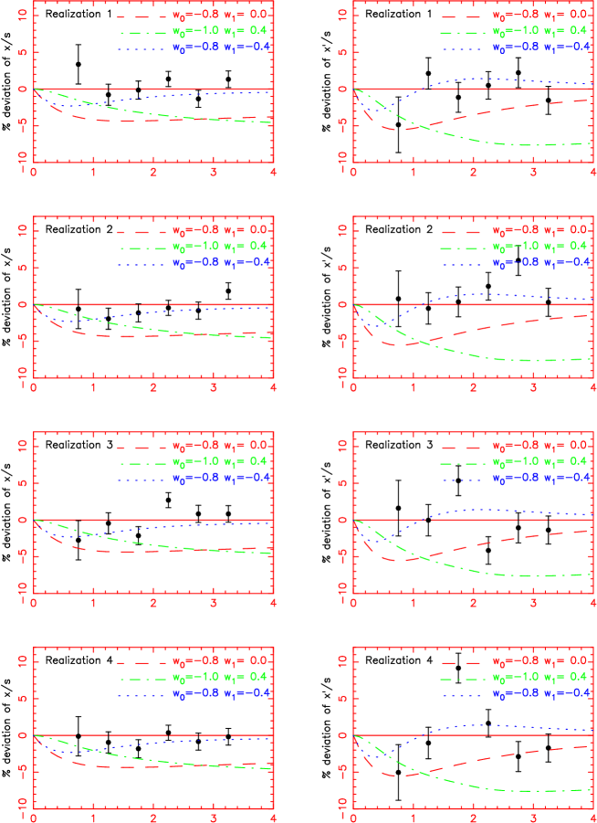
Figure 3: Simulated measurements of $x(z)/s$ and $x^{\prime}(z)/s$ in six redshift slices for the first four Monte Carlo realizations of a $1000$ deg² survey. The plotted values in each redshift bin are inferred from the fractional deviation of the fitted tangential and radial wavelengths from their fiducial values and the error bars represent the standard deviation across the realizations. The various model curves represent the fractional deviations of $x(z)$ and $x^{\prime}(z)$ as the dark energy model is varied from the fiducial point $(w_{0},w_{1})=(-1,0)$. The plots illustrate that these data would be sufficient to rule out dark energy parameters $(-0.8,0)$ and $(-1,0.4)$ with high confidence; but, owing to the cosmic degeneracy between $w_{0}$ and $w_{1}$, a model $(w_{0},w_{1})=(-0.8,-0.4)$ cannot be confidently excluded. Note that the evolution of $w(z)=w_{0}+w_{1}z$ is cut off at $z=z_{\rm cut}=2$.

Survey	Area	$z$-bin	Accuracy	Accuracy
	(deg2)		$x/s$ ($\%$)	$x^{\prime}/s$ ($\%$)
spec-$z$	1000	$0.5-1.0$	2.7	3.8
		$1.0-1.5$	1.4	2.1
		$1.5-2.0$	1.2	2.0
		$2.0-2.5$	1.0	1.9
		$2.5-3.0$	1.2	2.0
		$3.0-3.5$	1.1	1.9
spec-$z$	10000	$0.5-0.7$	1.7	2.7
		$0.7-0.9$	1.1	2.0
		$0.9-1.1$	1.0	1.5
		$1.1-1.3$	0.7	1.4
		$1.3-1.5$	0.6	1.2
KAOS	1000	$0.5-1.3$	1.6	2.6
	400	$2.5-3.5$	1.2	2.3
photo-$z$ $\sigma_{0}=0.03$	2000	$0.5-1.5$	2.3	–
		$1.5-2.5$	1.4	–
		$2.5-3.5$	1.3	–

Table 1: Simulated precision of recovery of the quantities $x(z_{\rm eff})/s$ and $x^{\prime}(z_{\rm eff})/s$ from a series of future spectroscopic and photometric redshift surveys. For spectroscopic redshift surveys, these quoted accuracies (for area $A_{1}$) may be approximately scaled to other survey areas ($A_{2}$) by multiplying by a factor $\sqrt{A_{1}/A_{2}}$ (since the errors in the power spectrum measurement $\delta P\propto 1/\sqrt{V}$). In order to scale the photometric redshift results to surveys with different r.m.s. redshift scatters $\sigma_{2}$, we can multiply by a further factor $\sqrt{\sigma_{2}/\sigma_{1}}$ (since the number of usable Fourier modes $m$ scales as $1/\sigma$, and $\delta P\propto 1/\sqrt{m}$). These simple scalings will break down (1) if the redshift range changes significantly, owing to the changing position of the non-linear transition, and (2) in the regime where we are just resolving the oscillations, when improvement is better than $\sqrt{V}$. The measurement precision of $x/s$ and $x^{\prime}/s$ is determined by Monte Carlo realizations and is accurate to $\pm$ 0.1%.

We parameterize the dark energy model using an equation-of-state $w(z)=w_{0}+w_{1}z$. The accuracies of $x(z)/s$ and $x^{\prime}(z)/s$ are then used to infer joint constraints over a grid of $(w_{0},w_{1})$, using the standard formulae for $x^{\prime}(z)=c/H(z)$ and $x(z)=\int_{0}^{z}x^{\prime}(z^{\prime})\,dz^{\prime}$, where the Hubble constant $H(z)$ at redshift $z$ is a function of $(\Omega_{\rm m},h,w_{0},w_{1})$. For the sound horizon $s$ we used the formulae of Efstathiou & Bond (1999, equations 18-20) in terms of $(\Omega_{\rm m},\Omega_{\rm b},h)$ so we effectively assume that the effect of dark energy at early times is insignificant. We explore a range of uncertainties for these quantities below. For each grid point in the $(w_{0},w_{1})$ plane we derive a likelihood for each redshift slice by marginalizing over Gaussian priors for $\Omega_{\rm m}$ and $\Omega_{\rm m}h^{2}$ (the natural variables – see below) centered upon $\Omega_{\rm m}=0.3$ and $h=0.7$. The sound horizon is only weakly dependent on $\Omega_{\rm b}$, therefore we simply fixed the value $\Omega_{\rm b}h^{2}=0.022$ (we checked that the likelihood contours remained unchanged for reasonable variations in $\Omega_{\rm b}h^{2}$). The overall $(68\%,95\%)$ likelihood contours were then determined by multiplying together the individual likelihoods inferred from the measurements of $x(z)/s$ and $x^{\prime}(z)/s$ for each redshift slice.

Figure 4 displays the resulting $(w_{0},w_{1})$ contours for a $10{,}000$ deg² survey. A further approximation has been used to generate this plot (also tested in the Appendix): that the accuracies of the fitted wavelengths determined for the $1000$ deg² simulation (Figure 3) may be scaled by a factor $\sqrt{10}$. This is simply equivalent to sub-dividing the $10{,}000$ deg² survey into $10$ separate independently-analyzed pieces. If we do not make this additional approximation, unfeasibly large Fourier transforms are required to handle the size of the survey cuboid. Furthermore, the statistical independence of $x(z_{\rm eff})$ and $x^{\prime}(z_{\rm eff})$ in a given redshift slice becomes weaker, as this independence rests upon the flat-sky approximation.

We note that:

1. There is a significant degeneracy in each redshift slice between $w_{0}$ and $w_{1}$, because approximately the same cosmology is produced if $w_{0}$ becomes more negative and $w_{1}$ becomes more positive. The axis of degeneracy is a slow function of redshift, which improves this situation somewhat as we combine different redshift slices.

2. As redshift increases, the radial oscillations provide decreasingly powerful constraints upon the dark energy model, because $H(z)$ becomes independent of $(w_{0},w_{1})$. This conclusion is valid if we are perturbing about the cosmological constant model $(-1,0)$, but will not be true in general for models with $w_{1}\neq 0$ for which dark energy may affect dynamics at higher redshift.

3. The tightness of the likelihood contours in the $(w_{0},w_{1})$ plane depends significantly upon the fiducial dark energy model (see Figure 14). As $w_{0}$ and $w_{1}$ become more positive, dark energy grows more influential at higher redshifts and the simulated surveys constrain the dark energy parameters more accurately, despite the fact that the surveyed cosmic volume is decreasing.

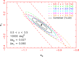
Figure 4: Likelihood contours for dark energy model parameters $(w_{0},w_{1})$ for a $10{,}000$ deg² survey. Contours are shown for six individual redshift slices ranging from $z=0.5$ to $z=3.5$ ($68\%$), together with the combined result ($68\%$,$95\%$). For this plot, precise knowledge of $\Omega_{\rm m}$ ($=0.3$), $h$ ($=0.7$) and $\Omega_{\rm k}$ ($=0$) is assumed. In Figures 5 and 6 we plot sets of contours for different priors in $\Omega_{\rm m}$, $h$ and $\Omega_{\rm k}$. The quoted errors $\Delta w_{0}$ and $\Delta w_{1}$ are produced by marginalizing over the other dark energy parameter (i.e. $w_{1}$ and $w_{0}$, respectively). This plot is obtained by scaling the inferred measurement accuracies of $x/s$ and $x^{\prime}/s$ from a $1000$ deg² simulation by a factor $\sqrt{10}$.

When generating Figure 4, we assume that the values of $\Omega_{\rm m}$ ($=0.3$) and $h$ ($=0.7$) are known perfectly. Although there is some useful cancellation between the trends of the distance scale $x(z)$ and the standard ruler scale $s$ with the value of $\Omega_{\rm m}h^{2}$, there is nevertheless some residual dependence of the experimental performance on the accuracy of our knowledge of both $\Omega_{\rm m}$ and $h$, independently.

In this paper we choose not to combine our results with cosmological priors from specific proposed experiments (as could be achieved by combining Fisher matrix information, for example). We prefer to keep our presentation in general terms by marginalizing over different priors for $\Omega_{\rm m}$ and $h$. We recognize that this approach will not capture all the parameter degeneracies inherent in future CMB, large-scale structure or supernova surveys, but nevertheless we can robustly quantify the accuracy of knowledge required for these other cosmological parameters such that their uncertainities do not dominate the resulting error in dark energy parameters. Combinations with any specific future experiment can be achieved by using our results listed in Table 1 which represent the fundamental observables recovered by this method: $x(z)$ and $x^{\prime}(z)$ in units of the sound horizon.

In general terms, one degree of freedom in other parameters is constrained by the excellent measurement of the physical matter density $\Omega_{\rm m}h^{2}$ afforded by the CMB angular power spectrum: accuracies of about $3\%$ ($\sigma(\Omega_{\rm m}h^{2})\approx 0.004$) and $1\%$ ($\sigma(\Omega_{\rm m}h^{2})\approx 0.001$) are possible with the WMAP and Planck satellites, respectively (Balbi et al., 2003). However, a second independent constraint on a combination of $\Omega_{\rm m}$ and $h$ is also required.

This is illustrated by Figure 5, in which we re-compute the overall likelihoods in the $(w_{0},w_{1})$ plane, marginalizing over the WMAP and Planck errors in $\Omega_{\rm m}h^{2}$ together with a second independent Gaussian prior on $\Omega_{\rm m}$. We conclude that for a survey of $10{,}000$ deg², $\Omega_{\rm m}$ must be known with an accuracy $\sigma(\Omega_{\rm m})\simeq 0.01$ (in conjunction with the WMAP or Planck determination of $\Omega_{\rm m}h^{2}$) in order that this uncertainty is not limiting. Note that as the cosmic volume surveyed increases, the prior requirements of knowledge of $\Omega_{\rm m}$ become more stringent. For a $1000$ deg² experiment, only $\sigma(\Omega_{\rm m})\lesssim 0.03$ is required (see Figure 10).

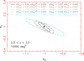
Figure 5: Likelihood contours ($68\%$) for dark energy model parameters $(w_{0},w_{1})$ for the same (combined) survey as Figure 4, considering various different Gaussian priors upon the values of $\Omega_{\rm m}h^{2}$ and $\Omega_{\rm m}$, with standard deviations $\sigma(\Omega_{\rm m}h^{2})$ and $\sigma(\Omega_{\rm m})$. We assume $\Omega_{\rm k}=0$. For the values of $\sigma(\Omega_{\rm m}h^{2})$ we make assumptions representative of the WMAP and Planck CMB experiments, for each of these cases we further consider $\sigma(\Omega_{\rm m})=0.01$ and $0.03$. For a survey of $10{,}000$ deg² covering redshift range $0.5<z<3.5$, WMAP suffices to determine the value of $\Omega_{\rm m}h^{2}$, but we require an independent constraint $\sigma(\Omega_{\rm m})\simeq 0.01$ in order that this uncertainty is not limiting.

Large-scale structure and/or supernovae constraints together with the first-year WMAP CMB data currently deliver $\sigma(\Omega_{\rm m})\approx 0.02$–0.04 assuming a flat Universe (e.g. Spergel et al., 2003; Tegmark et al., 2004; Cole et al., 2005). Balbi et al. (2003) quote $\sigma(h)\simeq 0.02$ as attainable with Planck (equivalent to $\sigma(\Omega_{\rm m})\simeq 0.02$), even allowing for uncertainty in the dark energy model. However, in light of Figure 5, this may not be sufficient for a $10{,}000$ deg² baryon oscillations survey.

Table 2 lists some $68\%$ confidence ranges for dark energy parameters $(w_{0},w_{1})$ for a range of survey configurations and cosmological priors, assuming a fiducial model $(-1,0)$.

Survey	Configuration	$\sigma(\Omega_{\rm m}h^{2})$	$\sigma(\Omega_{\rm m})$	$\sigma(w_{0})$	$\sigma(w_{1})$
spec-$z$	(10000 deg2, $0.5<z<3.5$)	0	0	0.03	0.06
		WMAP	0.01	0.04	0.07
		WMAP	0.03	0.08	0.10
		Planck	0.03	0.07	0.09
KAOS	(1000 deg2, $0.5<z<1.3$) + (400 deg2, $2.5<z<3.5$)	0	0	0.17	0.48
		WMAP	0.03	0.27	0.63
		WMAP	0.05	0.34	0.71
	($z\sim 1$) + (1000 deg2, $1.5<z<2.5$)	0	0	0.10	0.26
SKA	(20000 deg2, $0.5<z<1.5$)	0	0	0.04	0.11
		Planck	0.01	0.05	0.13
		Planck	0.03	0.11	0.18
photo-$z$	(10000 deg2, $0.5<z<3.5$, $\sigma_{0}=0.01$)	0	0	0.07	0.19
		WMAP	0.01	0.20	0.57
		WMAP	0.03	0.30	0.95
	(10000 deg2, $0.5<z<3.5$, $\sigma_{0}=0.03$)	0	0	0.12	0.32
		WMAP	0.01	0.23	0.66
		WMAP	0.03	0.31	0.95
	(2000 deg2, $0.5<z<3.5$, $\sigma_{0}=0.01$)	0	0	0.19	0.51
		WMAP	0.01	0.25	0.72
		WMAP	0.03	0.31	0.95

Table 2: Simulated $68\%$ confidence ranges for the dark energy parameters $(w_{0},w_{1})$ for a series of future spectroscopic and photometric redshift surveys, assuming a fiducial cosmology $(-1,0)$. A range of (Gaussian) priors on the values of $\Omega_{\rm m}h^{2}$ and $\Omega_{\rm m}$ are considered. The WMAP and Planck measurement precisions of $\sigma(\Omega_{\rm m}h^{2})$ are assumed to be $0.004$ and $0.001$, respectively. We assume $\Omega_{\rm k}=0$.

Throughout this paper we assume a spatially-flat ($\Omega_{\rm k}=0$) cosmology. In Figure 6 we compute how the likelihood contours in the $(w_{0},w_{1})$ plane for our $10{,}000$ deg² survey degrade as our knowledge of $\Omega_{\rm k}$ weakens. We note that current determinations of the curvature ($\sigma(\Omega_{\rm k})\lesssim 0.02$, Spergel et al., 2003; Eisenstein et al., 2005) are almost adequate for this proposed experiment. Of interest is Bernstein (2005) which noted that the the combination of baryon oscillations with weak lensing constraints leads to direct breaking of degeneracies of curvature with dark energy and allows $\Omega_{\rm k}$ to be measured without any assumptions about the equation of state.

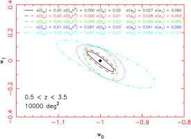
Figure 6: Likelihood contours ($68\%$) for dark energy model parameters $(w_{0},w_{1})$ for the same (combined) survey as Figure 4, considering various different Gaussian priors upon the value of $\Omega_{\rm k}=0$ with standard deviations $\sigma(\Omega_{\rm k})$. We consider both holding fixed the values of $\Omega_{\rm m}$ and $h$, and marginalizing over these parameters.

2.5 Comparison with the Fisher matrix methodology

It is worth comparing our methodology and results with the Fisher matrix approach utilized by Seo & Eisenstein (2003) for the simulation of baryonic oscillations experiments. The input data and assumptions are not entirely consistent in the two cases, but we can make a reasonably direct comparison of, for example, Figure 5 in Seo & Eisenstein (2003) with Figure 9 in this study. In such comparisons we find that the accuracies of determination of $(w_{0},w_{1})$ are consistent within a factor of about $1.5$, with the Fisher matrix method yielding tighter contours.

This is not surprising: the Fisher matrix method uses information from the whole power spectrum shape (which will also be distorted in an assumed cosmology, e.g. by the Alcock-Paczynski effect) whereas in our approach, this shape is divided out and only the oscillatory information is retained. The bulk of the Fisher information does appear to originate from the sinusoidal features (see Figure 5 in Hu & Haiman (2003) and Section 4.4 of Seo & Eisenstein (2003)). However, the improvement in dark energy precision resulting from fitting a full power spectrum template to the data may be up to $50\%$ compared to our ‘model-independent’ treatment. Our results should provide a robust lower limit on the accuracy, as intended.

We also note that the Fisher approach provides the minimum possible errors for an unbiased estimate of a given parameter based upon the curvature of the likelihood surface near the fiducial model. As a result the projected error contours for any combination of two parameters always form an ellipse (e.g. Figure 5 of Seo & Eisenstein (2003)). In our approach we explore the whole parameter space and estimate probabilities via Monte Carlo techniques: the error contours are thus larger and not necessarily elliptical (e.g. our Figure 9).

A further difference between the appearances of our Figure 9 and Figure 5 in Seo & Eisenstein (2003) is a noticeable change in the tilt of the principal degeneracy direction in the $(w_{0},w_{1})$ plane. The reason for this is readily identified: Seo & Eisenstein additionally incorporate the CMB measurement of the angular diameter distance to recombination into their confidence plots. We choose not to do this in order to expose the low redshift independent cosmological constraints from galaxy surveys and to isolate our results from the effects of any unknown behaviour of the equation of state (which could extend beyond our $w_{0},w_{1}$ formalism) between $z\sim 4$ and $z\sim 1100$.

In summary, we are encouraged by the rough agreement in values of $\Delta w_{0}$ and $\Delta w_{1}$ between these two very different techniques. They represent respectively more conservative/robust and best possible dark energy measurements from future surveys for baryon oscillations.

3 Detectability and accuracy of wavescale extraction

In this Section we take a step back from questions of dark energy and employ our simulation tools to re-consider the fundamental question of the detectability of the acoustic oscillations in $P(k)$ as a function of survey size and redshift coverage.

The oscillations in the galaxy power spectrum are a fundamental test of the paradigm of the origin of galaxies in the fluctuations observed in the early Universe via the CMB.

Detection of the oscillations would be an extremely important validation of the paradigm. Furthermore our standard ruler technique cannot be confidently employed unless the sinusoidal signature in the power spectrum can be observed with a reasonable level of significance.

Recently, analysis of the clustering pattern of SDSS Luminous Red Galaxies at $z=0.35$ (a volume of $\sim 3.5V_{\rm Sloan}$) has yielded the first convincing detection of the acoustic signal and application of the standard ruler (Eisenstein et al., 2005). Although this survey does not have sufficient redshift reach to strongly constrain dark energy models, this result is an important validation of the technique. Analysis of the final database of the 2dF Galaxy Redshift Survey has also yielded some visual evidence for baryonic oscillations (Cole et al., 2005). Here we make the distinction between detection of oscillations and detection of a baryonic signal $\Omega_{\rm b}\neq 0$ in the clustering pattern: baryons produce an overall shape distortion in $P(k)$ as well as the characteristic pattern of oscillations. In this Section we define the ‘wiggles detectability’ as the confidence of rejection of a smooth ‘no wiggles’ model (i.e. the best-fitting smooth reference spectrum of step 12 in Section 2.2). This is a different quantity to the ‘$3.4$-sigma confidence’ of observing $\Omega_{\rm b}\neq 0$ reported by Eisenstein et al. (2005). However, the techniques roughly agree on the measurement accuracy of the standard ruler (see the discussion of SDSS LRGs in our Paper I, Figure 3).

Figure 7 tracks the detection significance against the percentage accuracy of recovery of the standard ruler for surveys covering three different redshift ranges: $0.25<z<0.75$, $0.75<z<1.25$ and $2.75<z<3.25$. The lines connect points separated by survey volume intervals of $1V_{\rm Sloan}$; the solid circles denote volumes $(2,5,10)\,V_{\rm Sloan}$. For the purposes of this Section, an angle-averaged (isotropic) power spectrum is used rather than a power spectrum separated into tangential and radial components. We also only consider the pure vacuum $\Lambda$CDM model: the detectability is primarily driven by the cosmic volume surveyed, which is a relatively slow function of dark energy parameters. The detection significance is calculated from the average over the Monte Carlo realizations of the relative probability $P_{\rm rel}$ of the smooth ‘no-wiggles’ model and best-fitting ‘wiggles’ model, where

$$P_{\rm rel}=\exp{[-(\chi^{2}_{\rm no-wig}-\chi^{2}_{\rm best-wig})/2]}$$ (3)

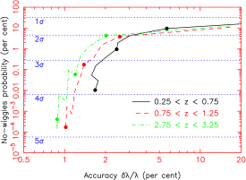
Figure 7: Variation of the ‘wiggles detectability’ (i.e. the significance of rejection of a no-wiggles model), and the accuracy with which the characteristic sinusoidal scale may be extracted, with survey volume. Three surveys are considered at different redshifts, centred upon $z=0.5$, $z=1$ and $z=3$. The lines join points separated by volume intervals of $1V_{\rm Sloan}$; the three solid circles on each line denote volumes $(2,5,10)\,V_{\rm Sloan}$.

We note that:

1. In order to obtain a significant ($3\sigma$) rejection of a no-wiggles model without using any power spectrum shape information, several $V_{\rm Sloan}$ must be surveyed. For the surveys centred at $z=(0.5,1,3)$ the required volume (in units of $V_{\rm Sloan}$) is approximately $(7,5,5)$. For the redshift ranges listed above, this corresponds to survey areas $(2300,700,500)$ deg².

2. For a fixed wiggles detection significance, the accuracy of recovery of the standard ruler increases with redshift. This is due to the larger available baseline in $k$ at higher redshift, owing to the extended linear regime. Two full oscillations are visible at $z=1$; four are unveiled by a survey at $z=3$.

3. For a fixed wavescale accuracy, the detection significance decreases with redshift, because the amplitude of the oscillations is damped with increasing $k$. As noted above, at higher redshifts there are more acoustic peaks available, thus a less significant measurement of each individual peak may be tolerated.

4. The distribution of values of $P_{\rm rel}$ (equation 3) over the Monte Carlo realizations is significantly skewed (see the discussion in Blake & Bridle (2005)). The median value of $P_{\rm rel}$ represents a more confident detection than the average plotted in Figure 7.

Figure 8 displays some Monte Carlo power spectrum realizations of three surveys: ($0.5<z<1.3$, $1000$ deg²), ($2.5<z<3.5$, $400$ deg²) and ($0.5<z<1.5$, $10{,}000$ deg²). The total volumes mapped in units of $V_{\rm Sloan}$ are $(10,8,133)$, respectively. The total numbers of galaxies observed in each survey (to ensure $n\times P=3$) are $(6,2,85)\times 10^{6}$ (assuming linear bias $b=3$ for the $z\sim 3$ survey and $b=1$ otherwise). The first two redshift surveys could be performed by a next-generation wide-field optical spectrograph such as the KAOS instrument proposed for the Gemini telescopes (Barden et al., 2004, http://www.noao.edu/kaos/). The third survey is possible in 6 months using the Square Kilometre Array to detect HI emission line galaxies (Abdalla & Rawlings, 2004) or from a space mission (see Section 4.4).

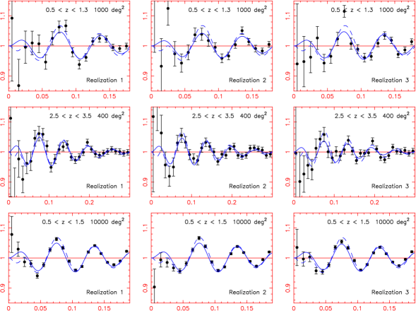
Figure 8: Power spectrum realizations of three example high-redshift surveys, varying survey volume and redshift range. In all cases, we plot the angle-averaged power spectrum divided by the smooth reference spectrum. The dashed curve is the theoretical input $P(k)$ and the solid line is the best fit of our simple decaying sinusoidal function (Paper I, equation 3). The $x$-axis is marked in units of $k$ (in $h$ Mpc^-1) and represents the extent of the linear regime at the redshift in question (i.e. $z_{\rm eff}=(z_{\rm min}+z_{\rm max})/2$). The rows of the Figure represent surveys with geometries ($0.5<z<1.3$, $1000$ deg²), ($2.5<z<3.5$, $400$ deg²) and ($0.5<z<1.5$, $10{,}000$ deg²); the columns display the first three Monte Carlo realizations in each case.

4 Dark energy measurements from realistic spectroscopic redshift surveys

We now consider the prospects of performing these experiments with realistic galaxy redshift surveys. As noted above and in Paper I, such surveys must cover a minimum of several hundred deg² at high redshift, cataloguing at least several hundred thousand galaxies, in order to obtain significant constraints upon the dark energy model.

4.1 Existing surveys

These requirements are orders of magnitude greater than what has been achieved to date. Some existing surveys of high-redshift galaxies are the Canada-France Redshift Survey (CFRS; a few hundred galaxies covering $\sim 0.1$ deg² to $z\approx 1.3$; Lilly et al., 1995), the survey of $z\sim 3$ Lyman-break galaxies by Steidel et al. (2003) (roughly a thousand galaxies across a total area $\approx 0.4$ deg²). Most other high redshift spectroscopic surveys (e.g. Abraham et al., 2004; Cimatti et al., 2002; Steidel et al., 2004) cover equally small areas $\lesssim 1$ deg².

Some larger surveys are in progress: the DEEP2 project (Davis et al., 2003), using the DEIMOS spectrograph on the Keck telescope, aims to obtain spectra for $60{,}000$ galaxies ($3.5$ deg², $0.7<z<1.4$); the VIRMOS redshift survey (Le Fevre et al., 2003), using the VIMOS spectrograph at the VLT, will map $150{,}000$ redshifts over $16$ deg² (considering the largest-area component of each). Neither of these existing projects comes close to meeting our goals, primarily due to the limitations of existing instrumentation. The spectrographs used to perform these surveys have typical fields-of-view (FOV) of diameter $10-20^{\prime}$ and are unable to cover hundreds of deg² in a reasonable survey duration.

4.2 New ground-based approaches (optical/IR)

Some proposed new optical instrumentation addresses this difficulty, permitting spectroscopic exposures over considerably larger FOVs using the 8-metre telescopes that are required to obtain spectra of sufficient quality at these redshift depths. For example, the KAOS project for the Gemini telescopes (Barden et al., 2004, http://www.noao.edu/kaos/) is a proposal for a $1.5$ deg diameter FOV, 4000 fibre-fed optical spectrograph. There are two proposed redshift surveys: $900{,}000$ ($0.5<z<1.3$) galaxies over $1000$ deg², and $600{,}000$ ($2.5<z<3.5$) galaxies across $400$ deg². These surveys would together take $\sim 170$ clear nights using the 8-metre Gemini telescope with realistic exposure times computed for the KAOS instrument sensitivity. The redshift ranges are driven by the strong spectral features available for redshift measurement in optical wavebands in a relatively short exposure time. The $z\sim 1$ range is cut off at $z=1.3$ by the [OII] emission line and the calcium H & K lines shifting to red/infrared wavelengths $>0.9$ µm where the airglow is severe and conventional CCD detectors have low efficiency; the $z\sim 3$ component is driven by observing Ly$\alpha$ in the blue part of the optical range.

The $w(z)$ measurements resulting from the proposed KAOS surveys, computed using the methodology of Section 2, are displayed in Figure 9 (see also Tables 1 and 2). We show both the $z\sim 1$ and $z\sim 3$ contributions separately, and the joint constraint. We assume linear bias factors $b=(1,3)$ for the $z\sim(1,3)$ simulations, respectively. The measurement precision of the dark energy parameters is $\Delta w_{0}\approx 0.2$ and $\Delta w_{1}\approx 0.4$, significantly better than current supernovae constraints (Riess et al., 2004). In statistical terms the KAOS performance is somewhat poorer than that projected for the proposed SNAP mission (Aldering et al., 2002), but the acoustic oscillations method is significantly less sensitive to errors of a systematic nature. Figure 9 illustrates that models with $w_{1}<0$ are harder to exclude owing to the diminishing sensitivity of cosmic distances to dark energy in this region of parameter space.

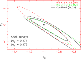
Figure 9: Measurement of a dark energy model $w(z)=w_{0}+w_{1}z$ using a simulated survey with the KAOS spectrograph consisting of two components, $0.5<z<1.3$ ($1000$ deg²) and $2.5<z<3.5$ ($400$ deg²). Constraints are displayed for each redshift component ($68\%$), and for both surveys combined ($68\%,95\%$). Note that the likelihoods are generated over a much wider $(w_{0},w_{1})$ space than displayed in the Figure. The solid circle denotes the fiducial cosmology, $(w_{0},w_{1})=(-1,0)$. There is a significant degeneracy between $w_{0}$ and $w_{1}$, particularly for the $z\sim 3$ survey if $w_{1}<0$, owing to the lack of sensitivity of $H(z=3)$ to dark energy in this case. For this plot, perfect knowledge of $\Omega_{\rm m}$ ($=0.3$), $h$ ($=0.7$) and $\Omega_{\rm k}$ ($=0$) is assumed. The standard deviations quoted for $\Delta w_{0}$ and $\Delta w_{1}$ (i.e. half the interval between the $16^{\rm th}$ and the $84^{\rm th}$ percentiles) result from marginalizing over the other parameter (i.e. $w_{1}$ and $w_{0}$, respectively).

We note that the KAOS measurement of $H(z\approx 3)$ from the radial component of the $z\sim 3$ power spectrum provides little information about the dark energy model if we are perturbing around the cosmological constant: at $z\sim 3$, the dynamics of the Universe are entirely governed by the value of $\Omega_{\rm m}h^{2}$, and $H(z)$ is almost independent of $(w_{0},w_{1})$. However, the value of $x(z\approx 3)$ inferred from the tangential component of the $z\sim 3$ power spectrum does depend on dark energy, because $x(z=3)$ is an integral of $dx/dz=c/H(z)$ from $z=0$ to $z=3$, which is influenced by dark energy at lower redshifts. The $z\sim 3$ constraint thus reduces to a significant degeneracy between $w_{0}$ and $w_{1}$, as observed in Figure 9, although models with $w_{1}>0$ can still be ruled out by this redshift component. The degeneracy is less severe for the $z\sim 1$ component owing to the availability of both $H(z)$ and $x(z)$ information.

Figure 9 assumes that we have perfect prior knowledge of $\Omega_{\rm m}$ ($=0.3$) and $h$ ($=0.7$). Figure 10 relaxes this assumption, illustrating the effect of including Gaussian priors upon $\Omega_{\rm m}$ and $\Omega_{\rm m}h^{2}$ of various widths.

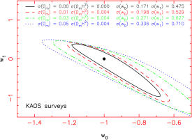
Figure 10: Likelihoods contours ($68\%$) of dark energy parameters $(w_{0},w_{1})$ for the same KAOS redshift surveys as Figure 9, marginalizing over the cosmological parameters $(\Omega_{\rm m},\Omega_{\rm m}h^{2})$. We assume a WMAP Gaussian prior upon $\Omega_{\rm m}h^{2}$ (as in Figure 5) and consider a range of different Gaussian priors for $\Omega_{\rm m}$. In each case, standard deviations are quoted for $w_{0}$ and $w_{1}$ as before. We assume $\Omega_{\rm k}=0$.

A drawback of this survey design is the absence of the redshift range $1.5<z<2.5$, sometimes called the ‘redshift desert’. There are no strong emission lines accessible to optical spectrographs in this interval: existing surveys of this region have required very long exposure times to secure spectra (Abraham et al., 2004), but this could be remedied by near-IR or near-UV spectroscopy of bright, star-forming galaxies (Steidel et al., 2004). We now consider the usefulness of these additional observations as regards measuring dark energy, along with the observational practicalities.

First, we investigate the effect of this redshift range upon measurements of the dark energy model $w(z)=w_{0}+w_{1}z$ (assuming precise prior knowledge of $\Omega_{\rm m}$ and $h$ for the purposes of this comparison; Figure 10 indicates how accurately these parameters must be known in order that their uncertainty is not limiting). In Figure 11, we remove the $z=3$ component of the proposed KAOS experiment and extend the lower-redshift $1000$ deg² survey across the redshift range $1.5<z<2.5$, divided into two independent slices of width $\Delta z=0.5$. The likelihood constraints in $(w_{0},w_{1})$ space tighten appreciably, by a further factor of two, principally due to the $1.5<z<2.0$ component, for which $H(z)$ still yields useful information about $(w_{0},w_{1})$. In Figure 12 we add back in the $z=3$ data; the dark energy measurements do not significantly improve. We conclude that coverage of the redshift desert would be highly desirable if it could be achieved. Simply increasing the area of the $z\sim 3$ component does not help nearly as much ($\Delta w_{1}$ is improved by $\sim 25\%$ for 1000 deg² at $z\sim 3$). This simplistic analysis is of course no substitute for a proper survey optimization assuming fixed total time or cost.

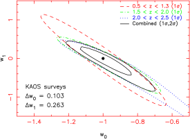
Figure 11: Dark energy measurements resulting from $1000$ deg² surveys spanning the redshift ranges ($0.5<z<1.3$) and ($1.5<z<2.5$). We assume perfect prior knowledge of $(\Omega_{\rm m},h,\Omega_{\rm k})$.

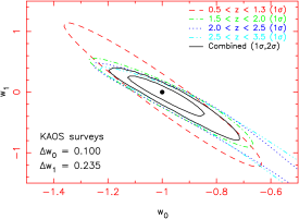
Figure 12: Dark energy measurements resulting from $1000$ deg² surveys spanning the redshift ranges ($0.5<z<1.3$) and ($1.5<z<2.5$), together with a $400$ deg² component covering ($2.5<z<3.5$). We assume perfect prior knowledge of $(\Omega_{\rm m},h,\Omega_{\rm k})$.

We note, however, that there are other persuasive scientific reasons to include a $z=3$ survey component (Eisenstein, 2002), amongst them:

1. A galaxy redshift survey at $z=3$ unveils the linear power spectrum down to unprecedentedly small scales $k\approx 0.5\,h$ Mpc^-1, measuring linear structure modes that cannot be accessed using the CMB.

2. If dark energy is insignificant at $z=3$, then measurement of the acoustic oscillations in such a redshift slice enables the standard ruler to be calibrated in a manner independent of the CMB.

3. Our present analysis assumes that the fiducial dark energy model is a cosmological constant, $(w_{0},w_{1})=(-1,0)$. Based on current data, we have very little information about the value of $w_{1}$ (for the latest supernova analysis of Riess et al. (2004), $\sigma(w_{1})\approx 0.9$). Should $w_{1}\neq 0$, the influence of $w(z)$ upon higher-redshift dynamics could become more significant. A general redshift survey optimization, which is beyond the scope of this paper, should address the range of $w(z)$ to be explored (Bassett et al., 2005).

Figure 13 considers a different parameterization for dark energy $w(z)=w_{0}+w_{a}(1-a)$ $=w_{0}+w_{a}/(1+z)$ (Linder 2002), where $a=(1+z)^{-1}$ is the usual cosmological scale factor, which encapsulates a more physically realistic behaviour at high redshifts $z\gtrsim 1$ in comparison to $w(z)=w_{0}+w_{1}z$. The rate of change of $w$ with redshift in the two models is $dw/dz=w_{1}=w_{a}/(1+z)^{2}<w_{a}$ hence for a given survey we expect the size of the error for $w_{a}$ to exceed that for $w_{1}$. Figure 13 illustrates this for the same survey configuration as Figure 12.

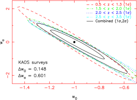
Figure 13: Dark energy measurements resulting from the same surveys as Figure 12, using the alternative parameterization $w(z)=w_{0}+w_{a}(1-a)$. We assume perfect prior knowledge of $(\Omega_{\rm m},h,\Omega_{\rm k})$. Note that the likelihoods are generated over a much wider $(w_{0},w_{a})$ space than displayed in the Figure.

Figure 14 uses the KAOS surveys plus a $1.5<z<2.0$ extension to illustrate how the tightness of the likelihood contours in the $(w_{0},w_{1})$ plane is a strong function of the fiducial dark energy parameters, as discussed in Section 2.3. We computed the linear growth factor for non-$\Lambda$CDM models by solving the appropriate second-order differential equation (e.g. Linder & Jenkins, 2003). If $w_{1}>0$ then dark energy is more significant at higher redshifts and the model parameters can be constrained more tightly, despite both the resulting decrease in the available cosmic volume in a given redshift range and the movement of the linear/non-linear transition to larger scales (smaller $k$). Note that our cut-off to the evolution of $w(z)=w_{0}+w_{1}z$ at $z_{\rm cut}=2$ ensures that dark energy does not dominate at high redshift for our model with $w_{1}>0$.

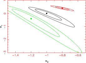
Figure 14: The tightness of the $(68\%,95\%)$ likelihood contours in the $(w_{0},w_{1})$ plane is a strong function of the fiducial cosmological model. In this Figure we illustrate, for three different fiducial models $(w_{0},w_{1})=(-1,0)$, $(-0.8,0.4)$ and $(-1.2,-0.4)$, dark energy measurements resulting from $1000$ deg² surveys spanning the redshift ranges ($0.5<z<1.3$) and ($1.5<z<2.0$), together with a $400$ deg² component covering ($2.5<z<3.5$). We assume perfect prior knowledge of $(\Omega_{\rm m},h,\Omega_{\rm k})$.

Next, we consider the practicalities of observing galaxies in the redshift range $1.5<z<2.5$ (the so-called ‘optical redshift desert’). Considering near infra-red wavebands first: the H$\alpha$ 6563Å line is accessible in the 1–2$\mu$m band over the interval $0.5<z<2$. This regime is the non-thermal infra-red, in which the sky is sufficiently dark to permit high-redshift spectroscopy (e.g. the emission-line observations of Glazebrook et al. (1999) and Pettini et al. (1998)). The critical opportunity offered here is that the H$\alpha$ emission line is potentially very bright at redshifts $z\gtrsim 1$, owing to the steep evolution in the star-formation rate of galaxies in the Universe over $0<z\lesssim 1$ (Hopkins, Connolly, & Szalay, 2000).

Let us consider a redshift slice $1.5<z<1.7$. Our requirement for shot noise sampling ($n\times P=3$) translates into a required surface density $(3900/b^{2})$ deg^-2 within this slab (Figure 1), where $b$ is the linear bias factor of the surveyed galaxies. The luminosity function of H$\alpha$ emitters at $z\gtrsim 1$ has been reasonably well determined from NICMOS slitless grism surveys using the Hubble Space Telescope (Hopkins, Connolly, & Szalay, 2000; Yan et al., 1999). Using the Hopkins et al. luminosity function, we find that we need to reach a line flux limit of $1.1\times 10^{-16}$ ergs cm^-2 s^-1 in order to reach the required surface density (assuming $b=1$). The $z=1$ H$\alpha$ luminosity function has apparently evolved strongly in comparison with $z=0$ (Gallego et al., 1995) but the measurements are fairly robust: we can double-check the luminosity function determinations by simply counting objects in the NICMOS surveys above our required line flux limit. In the Hopkins, Connolly & Szalay sample there are 4 galaxies in the redshift range $1.5<z<1.7$ above this flux limit, spread over 4.4 arcmin², yielding a surface density $\simeq$ 3300 deg^-2. The H$\alpha$ identifications are also very reliable: the Yan et al. sample was observed in optical wavebands by Hicks et al. (2002), confirming $\geq 75\%$ of the H$\alpha$ identifications via associated [OII] emission at the same redshift. This agrees with expectations: analytic models of evolving line emission show that H$\alpha$ should dominate at these flux levels at 1-2µm over other lines.

This is encouraging, because these bright lines are accessible in relatively modest exposures. Let us assume an 8-metre telescope, a $25\%$ efficient $R=4000$ near-IR spectrograph and detector (with a dispersion of 5Å per arcsec), and consider an object observed in an aperture of size 0.8 arcsec $\times$ 0.8 arcsec, covering $2\times 2$ pixels and containing half the light (the Yan et al. objects have compact half-light radii of 0.2–0.7 arcsec). The signal-to-noise ratio is determined by detector readout noise, sky background and dark current. We will assume a readout noise of 4 electrons (this is the stipulated requirement of the James Webb Space Telescope (JWST) detectors) and an inter-OH sky background of 1.2 photons s^-1 nm^-1 arcsec^-2 m^-2 in the H-band (the OH night sky line forest is well-resolved at $R=4000$) which is a typical value measured at Gemini observatory. We will neglect dark current, which is equivalent to assuming that this dark current is much lower than the sky counts. Given these assumptions, our H$\alpha$ flux limit at $z=1.6$ corresponds to a signal-to-noise ratio of 20 in a 600 second integration, and we find the observation is background limited for any readout noise $<$ 15 electrons.

This exposure time is encouragingly short, and implies that using a 1 degree FOV spectrograph, one could survey $1000$ deg² in only 20 nights. Admittedly our instrument specification is optimistic, especially for readout noise; however, it can be relaxed considerably whilst still achieving exposure times $<1$ hour. Assuming a fibre spectrograph we estimate that observing 3900 objects simultaneously at this resolution would only require 2–3 detector arrays of size 4096$\times$4096 to cover the $H$-band. Obviously more objects or broader wavelength coverage would require more detectors or time. Finally we note that, at least in principle, the exposure times are sufficiently short that one could imagine performing such a survey on a smaller-aperture (4-metre class) telescope.

The potential problem with the approach outlined above is that it is not known ‘a priori’ which of the galaxies identified in deep images will be H$\alpha$ bright, or the redshifts of these galaxies. Possibly these data could be successfully predicted from other information (e.g. broad-band colours or sub-mm/radio fluxes), but this may be unreliable. Targetting fainter H$\alpha$ fluxes resulting from realistic target selections would obviously require longer exposure times. Further work on this problem is required in order to determine the distinguishing properties of known H$\alpha$-bright galaxies.

A second potential difficulty is the effect of the night-sky OH emission lines in potentially making inaccessible certain redshift ranges, in a complex pattern. Since these redshift ranges are very narrow, the result is the removal of a series of redshift spikes at known locations in the radial window function. In order to assess the likely consequences, we manufactured a synthetic $n(z)$ possessing narrow gaps where no galaxies could be observed, i.e. when the redshifted H$\alpha$ emission line coincided with an OH line or landed in the water-absorption hole between the J and H bands. We assumed a spectrograph operating at a resolution $R=4000$, which implied that $68\%$ of the $1.1<z<1.7$ redshift interval was accessible. With our simulation tools we then recovered $P(k)$ using this $n(z)$ (employing an FFT with sufficient gridding in the radial direction to resolve these narrow spikes). The principal effect of the window function is to damp the amplitude of the acoustic oscillations slightly in the radial direction, leaving the tangential modes largely unaffected. The fractional error ($\Delta k_{A}/k_{A}$) with which the acoustic scale is recovered is increased by no more than $25\%$, which is mostly due to the smaller effective survey volume owing to the absence of many thin redshift shells. We conclude that the OH lines are not a factor which will significantly hamper ground-based surveys of the acoustic peaks.

Bright star-forming galaxies can alternatively be observed by targetting the [OII] 3727Å emission line in optical wavebands. High-resistivity CCD detectors under development can maintain quantum efficiency out to 1µm (Stover et al., 1998) corresponding to $z=1.7$. The typical H$\alpha$:[OII] intensity is 2:1; high spectral resolution is again required to observe between the OH night sky lines, in which case the exposure times would be short if one could pre-select the [OII]-bright population. This could be more problematic than with H$\alpha$ as there is considerable extra scatter introduced in to the line ratio [OII]$/$H$\alpha$ due to variations in metallicity and extinction (Jansen, Franx & Fabricant, 2001). We also note that [OII] is accessible in the non-thermal IR up to $z=5$ and therefore is a potential probe of high-redshift acoustic oscillations.

The high star-formation rate at earlier cosmic epochs also implies a considerable boost in the rest-frame UV luminosity of galaxies. High-altitude sites such as Mauna Kea have an atmospheric cutoff further into the near-UV, which can be exploited by blue-optimized spectrographs. For example, Steidel et al. (2004) have obtained spectra of star-forming galaxies over $1.4<z<2.5$ using exposure times of only a few hours at the 10-metre Keck telescope, reaching a lowest observed-frame wavelength of 3200Å; this corresponds to Ly$\alpha$ at $z=1.6$, or CIV at $z=1.1$. The spectral region between Ly$\alpha$ and CIV is rich in interstellar lines and ripe for determination of accurate redshifts. It is possible that a UV approach may be superior to a near-IR approach targetting H$\alpha$: the observed surface density of Steidel et al. sample is sufficiently high for our requirements, but we note that a UV-optimized design would probably require a wide-field slit spectrograph because conventional fibres considerably attenuate the UV light for long runs ($>20$m).

4.3 New ground-based approaches (radio)

Next-generation radio interferometer arrays, such as the proposed Square Kilometre Array (SKA; http://www.skatelescope.org; planned to commence operation in about 2015), will have sufficient sensitivity to detect the HI (21cm) transition of neutral hydrogen at cosmological distances that are almost entirely inaccessible to current radio instrumentation. This will provide a very powerful means of performing a large-scale redshift survey: once an HI emission galaxy has been located on the sky, the observed wavelength of the emission line automatically provides an accurate redshift.

The key advantage offered by a radio telescope is that it may be designed with an instantaneous FOV exceeding $100$ deg² (at $1.4$ GHz), vastly surpassing the possibilities of optical spectrographs. Equipped with a bandwidth of many $100$ MHz, such an instrument could map out the cosmic web (probed by neutral hydrogen) at an astonishing rate: the SKA, if designed with a large enough FOV, could locate $\sim 10^{9}$ HI galaxies to redshift $z\approx 1.5$ over the whole visible sky in a timescale of $\sim 1$ year (Abdalla & Rawlings, 2004; Blake et al., 2004). Deeper pointings could probe the HI distribution to $z\sim 3$ over smaller solid angles. A caveat is that the HI mass function of galaxies has been determined locally (Zwaan et al., 2003) but is currently very poorly constrained at high redshift. However, for a range of reasonable models, the number densities required to render shot noise negligible may be attained for HI mass limits larger than the break in the mass function (Abdalla & Rawlings, 2004). Another requirement of interferometer design is that a significant fraction of the collecting area must reside in a core of diameter a few km, to deliver the necessary surface brightness sensitivity for extended 21cm sources. Sharp angular resolution is not a pre-requisite, assuming that the observed galaxies are not confused.

Figure 15 displays measurements of the dark energy model resulting from a $20{,}000$ deg² neutral hydrogen survey over the redshift range $0.5<z<1.5$, analyzing acoustic peaks in redshift slices of width $\Delta z=0.2$. We note that a smaller 21cm survey could be performed in the nearer future by SKA prototypes such as the HYFAR proposal (Bunton et al., 2003), which may cover several thousand deg² over a narrower bandwidth (corresponding to $0.8<z<1.2$).

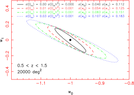
Figure 15: Likelihoods ($68\%$) of dark energy parameters $(w_{0},w_{1})$ for a future 21cm radio survey, using the Square Kilometre Array to map HI emission galaxies over $20{,}000$ deg², covering a redshift range $0.5<z<1.5$. Such a survey is possible in a timescale of less than 1 year if the SKA is designed with a sufficiently large FOV ($\sim 100$ deg² at $1.4$ GHz) and bandwidth ($\sim 200$ MHz). We marginalize over the cosmological parameters $(\Omega_{\rm m},\Omega_{\rm m}h^{2})$ using a range of different Gaussian priors. Our assumed prior for $\Omega_{\rm m}h^{2}$ is representative of that obtained by the Planck satellite. We assume $\Omega_{\rm k}=0$.

4.4 Space-based approaches

An interesting alternative approach is to use a space-based dispersive but slitless survey to pick out emission-line objects directly over a broad redshift range. In space, the 1–2$\mu$m background is $1000$ times lower (in a broad band) than that observed from the ground (based upon the JWST mission background simulator at distance 3 au from the Sun; Petro, Kriss & Stockman, 2002); in the background-limited regime this gain is equivalent to a $1000$-fold increase in collecting area. The dispersing element could be either a large objective prism or a grism. The NICMOS surveys mentioned above already demonstrate that this technique is possible, but they lack somewhat in FOV and spectral resolution compared to what is desirable.

As an illustrative example, let us consider a 0.5-metre space telescope with a $60\%$ overall system efficiency working in slitless dispersed imaging mode, again targeting $0.5^{\prime\prime}$ galaxies at redshift $z=1.6$. We will assume the JWST-like background and that the slitless spectra are de-limited by a 2000Å-wide blocking filter. Just considering the sky background, the signal-to-noise ratio in a 1800s exposure is 5 for our canonical flux limit of $1.1\times 10^{-16}$ ergs cm^-2 s^-1. This signal-to-noise ratio is independent of spectral resolution for unresolved lines much brighter than the continuum (the spectral resolution must of course be sufficient for determining accurate redshifts). Highly-dispersive IR materials such as silicon could enable an objective prism approach with $R=500$, using a simple prime focus imaging system. Such a satellite, if equipped with a 1 deg FOV and sensitive over 1–2µm, could perform a spectroscopic survey over the redshift interval $0.5<z<2$ (using H$\alpha$), covering an area of $10{,}000$ deg² in a 4 year mission, obtaining dark energy constraints very similar to those presented in Figure 4. Accessing higher redshifts would be possible by either extending the wavelength range or going fainter with the [OII] line, in both cases requiring a larger diameter mirror. Ambiguous line identification is a potential problem, this could be remedied by cross-matching with a photometric-redshift imaging survey. We refer the reader to Glazebrook et al. (2004) for a more detailed discussion of such a dedicated ‘Baryonic Oscillation Probe’.

5 Dark energy measurements from realistic photometric redshift surveys

We next explore the potential of surveys based on photometric redshifts for detecting the acoustic oscillations and placing constraints upon any cosmic evolution of the dark energy equation-of-state $w(z)$. For a detailed treatment of the significance of ‘wiggles detection’ and the accuracy of measurement of the standard ruler with photometric redshift surveys, we refer the reader to Blake & Bridle (2005). Here we present a summary and discuss the consequences for dark energy measurement.

A photometric redshift (‘photo-z’) is obtained from multi-colour photometry of a galaxy: the object is imaged in several broad-band filters, ranging from the UV to the near-IR, producing a rough spectral energy distribution (SED). This observed SED is then fitted by model galaxy SEDs as a function of redshift to construct a likelihood distribution with redshift; the peak of the likelihood function indicates the best-fitting redshift. A classic example of this approach is the analysis of the Hubble Deep Field North (Fernández-Soto, Lanzetta, & Yahil, 1999).

There are obviously many options concerning the number and width of filter bands, and their placement in the UV-NIR range. Generally at least five broad bands are used, and IR coverage is essential for constraining galaxies with $1.2<z<2.2$ (Bolzonella, Miralles, & Pelló, 2000). Some approaches have used as many as 17 broad $+$ narrow-band filters (e.g. Wolf et al., 2003). Many different techniques have been proposed for deriving the photo-z (e.g. Csabai et al., 2000; Le Borgne & Rocca-Volmerange, 2002; Collister & Lahav, 2004). The important question for our study is: what is the accuracy of the photo-z estimates?

These errors can be divided into two main types. First, there is the random statistical error due to noise in the flux estimates and to the coarseness of the SED. Typically this is specified by a parameter $\sigma_{0}$ where

$$\sigma_{0}={\sigma_{z}\over(1+z)}\approx\hbox{constant}$$ (4)

and $\sigma_{z}$ is the standard deviation of the redshift $z$. We note that $\sigma_{0}$ is approximately constant because it is proportional to the spectral resolution $\lambda/\Delta\lambda$ of the set of filters. Chen et al. (2003) obtained $\sigma_{0}=0.08$; the COMBO17 survey achieved $\sigma_{0}=0.03$. In a theoretical study, Budavári et al. (2001) demonstrated that an optimized filter set produced results within the range $\sigma_{0}=0.02-0.05$, depending on the shape of the SED. In general, redder galaxies deliver more accurate photo-z’s because the model colours change faster with redshift.

The second source of photo-z error is the possibility of getting the redshift grossly wrong, either because the set of colours permit more than one redshift solution, or because the model SEDs are not sufficiently representative of real galaxies. Different authors disagree about the magnitude of this effect, which depends on the specific filter sets, photometric accuracy, spectroscopic calibration and photo-z methods used. A useful theoretical discussion is given in Bolzonella, Miralles, & Pelló (2000). Blake & Bridle (2005) analyze various ‘realistic’ redshift error distributions including outliers and systematic offsets.

For our purposes we will ignore systematic errors and parameterize photo-z performance using the value of $\sigma_{0}$ alone. A realistic survey will contain additional systematic redshift errors, thus we will obtain lower limits. We will also assume that $\sigma_{0}$ is a constant, whereas for a realistic survey it will depend somewhat on redshift and galaxy type.

What is the effect of a statistical redshift error ($\sigma_{0}$) on the measured power spectrum? This is fairly easy to estimate analytically. As discussed in Paper I (see also Seo & Eisenstein, 2003, Section 4.5) this photo-z error represents a radial smearing of galaxy positions. For example, $\sigma_{0}=0.03$ for a $z=1$ galaxy corresponds to an error $\sigma_{x}\approx 100\,h^{-1}$ Mpc in the radial co-moving coordinate. Since smoothing (i.e. convolution) by a Gaussian function in real space is equivalent to multiplication by a Gaussian function in Fourier space, we can model the photo-z effect as a multiplicative damping of the 3D power spectrum $P(k_{x},k_{y},k_{z})$ by a term $\exp{(-k_{x}^{2}\sigma_{x}^{2})}$ (where we choose the $x$-axis as the radial direction). In the following, we implement a flat-sky approximation and presume that there is no tangential effect (i.e. parallel to the $(y,z)$-plane).

Prior to the smearing effect of photometric redshifts, the available Fourier structure modes in the linear regime comprise a sphere in Fourier space of radius $k<k_{\rm linear}\approx 0.2\,h$ Mpc^-1 (where the value of $k_{\rm linear}$ depends on redshift). Afterwards, the damping term $\exp{(-k_{x}^{2}\sigma_{x}^{2})}$ implies that only a thin slice of this sphere with $|k_{x}|\lesssim 2/\sigma_{x}\approx 0.02\,h$ Mpc^-1 is able to contribute useful power spectrum signal. This is illustrated schematically in Figure 16. Considering those modes contributing to a Fourier bin centred about scale $k$, the reduction in usable Fourier space volume corresponds to a factor $(k\times\sigma_{x}/2)$. At a scale $k=0.2\,h$ Mpc^-1, this represents a loss by a factor of 10 ($\sigma_{0}=0.03$, $z=1$). For the same surveyed area, we can hence expect the error ranges in the derived power spectrum to worsen by a factor $\approx\sqrt{10}$ in comparison to a spectroscopic survey (although also note that the scaling of the error with $k$ also changes from $\delta P_{\rm spec}\propto k^{-1}$ to $\delta P_{\rm photo}\propto k^{-1/2}$). The errors on the resulting dark energy parameters will be worse by a factor of $\simeq\sqrt{20}$ than in a similar sized spectroscopic survey once one also accounts for the loss on the radial dimension.

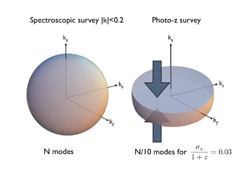
Figure 16: Illustration of the loss of modes in three dimensional Fourier space $(k_{x},k_{y},k_{z})$ by smearing along the $x$ (redshift) axis. Only long-wavelength modes $>$ smearing length are unsuppressed and the $|k|<0.2$ sphere is truncated to a thin disk.

Critically, the radial damping due to photometric redshifts results in the loss of any ability to detect the acoustic oscillations in the radial component of the power spectrum (in the above example, the power spectrum is significantly suppressed for modes with $|k_{x}|>2/\sigma_{x}\approx 0.02\,h$ Mpc^-1, i.e. the whole regime containing the oscillations). We are only able to apply the standard ruler in the tangential direction. As noted earlier, the radial component provides a direct measure of $H(z)$, contributing significantly to the measurements of the dark energy model. Thus in the above example ($\sigma_{0}=0.03$, $z=1$) the resulting errors in the dark energy parameters will worsen by a factor closer to $\approx\sqrt{20}$. Alternatively, one could compensate by increasing the survey area (and hence the density of states in Fourier space) by the corresponding factor. We note that with sufficient filter coverage and for special classes of galaxy, the photometric redshift error $\sigma_{0}$ may also be reduced to improve dark energy performance.

We simulated photo-z surveys using analogous Monte Carlo techniques to those described in Section 2 (see Blake & Bridle (2005) for a more detailed account). We introduced a radial Gaussian smearing

$$\sigma_{x}=\sigma_{0}\,(1+z_{\rm eff})\,x^{\prime}(z_{\rm eff})$$ (5)

into our Poisson-sampled density fields (for a survey slice at redshift $z_{\rm eff}$). When measuring the power spectrum we restrict ourselves to modes with $|k_{x}|<2/\sigma_{x}$ (where the factor of 2 was determined empirically to be roughly optimal). The residual damping in the shape of $P(k)$ is divided out using the known Gaussian damping expression. We bin the power spectrum modes in accordance with the total length of the Fourier vector $k=\sqrt{k_{x}^{2}+k_{y}^{2}+k_{z}^{2}}$, noting that only tangential modes (with $k_{x}\approx 0$) are being counted. We fit a 1D decaying sinusoid (Paper I, equation 3) to the result. The scatter of the fitted wavescales across the Monte Carlo realizations is interpreted as the accuracy of measurement of the quantity $x(z_{\rm eff})/s$ (given that only tangential modes are involved). We uniformly populated our survey volumes such that $n\times P=3$.

We consider two different photo-z accuracies: $\sigma_{0}=0.03$, representing the typical fidelity of the current best photo-z studies, and $\sigma_{0}=0.01$, which we somewhat arbitrarily adopt as an upper limit to future improvements. Blake & Bridle (2005) consider a much wider range of possibilities. We note that in our methodology, reducing the value of $\sigma_{0}$ by some factor is equivalent to covering a proportionately larger survey area. Figure 17 displays some Monte Carlo realizations of measured power spectra for these photometric redshift surveys, assuming a redshift range $0.5<z<1.5$. We assume a survey solid angle of $10{,}000$ deg², but also consider a smaller project ($2000$ deg² with $\sigma_{0}=0.01$).

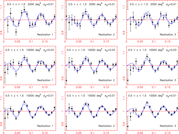
Figure 17: Power spectrum realizations for three example photometric redshift surveys, varying survey area and photo-z accuracy (parameterized by $\sigma_{0}$). In all cases we assume a survey redshift interval $0.5<z<1.5$ (i.e. $z_{\rm eff}=1$). Only radial Fourier modes with $|k_{x}|<2/\sigma_{x}$ (where $\sigma_{x}=\sigma_{0}\,(1+z_{\rm eff})\,x^{\prime}(z_{\rm eff})$) are binned when measuring $P(k)$, which is plotted divided by a smooth reference spectrum. As in Figure 8, the dashed curve is the theoretical input $P(k)$ and the solid line is the best fit of our simple decaying sinusoidal function (Paper I, equation 3). The $x$-axis is marked in units of $k$ (in $h$ Mpc^-1) and represents the extent of the linear regime at redshift $z_{\rm eff}$. The rows of the Figure represent surveys with parameters ($2000$ deg², $\sigma_{0}=0.01$), ($10{,}000$ deg², $\sigma_{0}=0.03$) and ($10{,}000$ deg², $\sigma_{0}=0.01$); the columns display the first three Monte Carlo realizations in each case.

Figure 18 illustrates the resulting measurement of the dark energy parameters $(w_{0},w_{1})$ for these survey configurations, assuming that we can span the redshift range $0.5<z<3.5$ (also see Tables 1 and 2). These $(w_{0},w_{1})$ contours are computed using the same method as Section 2.4, utilizing measurements of $x(z)/s$ in three redshift bins of width $\Delta z=1$ (for real data, narrower redshift slices would be used and the results co-added). Each of these redshift constraints corresponds to a degenerate line in the $(w_{0},w_{1})$ plane (i.e. constrains one degree of freedom in the dark energy model) but, as described in Section 2.4, the direction of degeneracy slowly rotates with redshift: the combination of the likelihoods for each redshift bin results in closed contours.

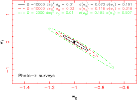
Figure 18: Dark energy measurements resulting from three different photometric redshift surveys covering the interval $0.5<z<3.5$. We assume perfect prior knowledge of $(\Omega_{\rm m},h,\Omega_{\rm k})$. Table 2 lists results for a range of different priors.

Note that for photometric redshift surveys, the cosmological priors on $\Omega_{\rm m}h^{2}$ and $\Omega_{\rm m}$ required to achieve a given measurement precision of $(w_{0},w_{1})$ are much tighter than for spectroscopic surveys (see Table 2). This is because in the absence of $H(z)$ information, the photo-$z$ survey must achieve a significantly tighter measure of $x(z)$ to recover a corresponding measurement accuracy of the dark energy parameters, rendering it more susceptible to uncertainties in $\Omega_{\rm m}$ and $h$.

The real figure-of-merit for comparison of practical instruments is the accuracy with which the dark energy model can be measured for a fixed total observing time or at a fixed cost. The myriad details of comparing large imaging cameras with large spectroscopic systems are beyond the scope of this paper. However, we note that the proposed Large Synoptic Survey Telescope (LSST; Tyson, 2002) could image half of the entire sky to the required depth ($V\approx 25$) in multiple colours every 25 nights; such a survey would produce dark energy constraints comparable with a spectroscopic (e.g. KAOS) survey of 1000 deg² (the latter requiring 170 nights) if $\sigma_{0}=0.01$ could be achieved. We regard this level of photometric redshift accuracy as unlikely for ground-based surveys. We note that the KAOS measurements additionally constrain $H(z)$ leading to qualitatively more robust measurement of dark energy. Further the KAOS survey could be improved by adding more area, whereas once the LSST has observed the whole celestial hemisphere, there is obviously no further gain in $w(z)$ information from further passes. However, since ‘all-sky’ deep multi-colour surveys are being performed for other scientific reasons (e.g. cosmic shear analysis), it is of considerable value to utilize these data for baryonic oscillation studies. Furthermore, as discussed in detail by Blake & Bridle (2005), a photometric redshift survey of several thousand square degrees may provide constraints competitive with spectroscopic surveys in the short term.

6 Conclusions

This study has extended the methodology of Blake & Glazebrook (2003) to simulate measurements of the cosmic evolution of the equation-of-state of dark energy $w(z)$ from the baryonic oscillations, using the simple parameterization $w(z)=w_{0}+w_{1}z$. The methodology used is very similar to that of Paper I, treating the primordial baryonic oscillations in the galaxy power spectrum as a standard cosmological ruler, whilst dividing out the overall shape of the power spectrum in order to maximize model-independence. In this study we make the improvement of fitting independent radial and tangential wavescales, showing that this is directly equivalent to measuring $D_{A}(z)$ and $H(z)$ in a series of redshift slices in units of the sound horizon. This results in improved constraints upon $(w_{0},w_{1})$. We have tested the approximations encoded in our approach and found them all to be satisfactory, increasing our confidence in the inferred error distributions for the dark energy parameters. The simulated accuracies for $(w_{0},w_{1})$ are roughly consistent with other estimates in the literature based on very different analysis methods.

Our baseline ‘KAOS-like’ optical surveys of $\sim 1000$ deg², which can be realized by the next generation of spectroscopic instruments at ground-based observatories, deliver measurements of the dark energy parameters with precision $\Delta w_{0}\approx 0.15-0.2$ and $\Delta w_{1}\approx 0.3-0.4$. In statistical terms, these constraints are poorer than those which may be provided by a future space-based supernova project such as the SNAP proposal. We note, however, that the baryonic oscillations method appears to be substantially free of systematic error, with the principal limitation being the amount of cosmic volume mapped. In addition, any measurement of deviations from a cosmological constant model is of sufficient importance for physics that entirely independent experiments would be demanded to confirm the new model. A next-generation radio telescope with a FOV $\approx 100$ deg² at $1.4$ GHz, performing a redshift survey of 21cm emission galaxies over several $1000$ deg², may be available on a similar timescale.

We have considered the observational possibilities of more extensive baryonic oscillation experiments covering a significant fraction of the whole sky. Such a survey (encompassing $0.5<z<3.5$) may be straight-forward using a dedicated several-year space mission with slitless spectroscopy. In radio wavebands, the Square Kilometre Array would be able to survey the entire visible sky out to $z\approx 1.5$ in 6 months, if equipped with a sufficiently large FOV. These experiments would deliver extremely precise measurements of the dark energy model with accuracy $\Delta w_{0}\approx 0.03-0.05$ and $\Delta w_{1}\approx 0.06-0.1$ and would be invaluable to pursue if a significant non-vacuum dark energy signal was detected by smaller surveys.

We have also explored in detail the potential of photometric redshift optical imaging surveys for performing baryonic oscillations experiments. The loss of the radial oscillatory signal, due to the damping caused by the redshift errors, implies that we can no longer recover information about the Hubble constant at high redshift. However, the baryonic oscillations can still be measured using tangential Fourier modes. A deep $2000$ deg² imaging survey with excellent photometric redshift precision ($\sigma_{0}<0.03$) would allow the oscillations to be detected (2.5$\sigma$ significance). Useful constraints upon the dark energy model are possible if $\sim 20{,}000$ deg² can be surveyed (such an experiment with $\sigma_{0}=0.03$ is roughly equivalent to a $\sim 1000$ deg² spectroscopic survey).

We conclude that the baryonic oscillations in the clustering power spectrum represent one of the rare accurate probes of the cosmological model, possessing the potential to delineate cleanly any cosmic evolution in the equation-of-state of dark energy, via accurate measurements of $D_{A}(z)$ and $H(z)$ in a series of redshift slices. Importantly, such an experiment is likely to be substantially free of systematic error. Recent observations of SDSS Luminous Red Galaxies at $z=0.35$ have provided the first convincing detection of the acoustic signature and validation of the technique. The challenge now is to create the large-scale surveys at higher redshifts required for mapping the properties of the mysterious dark energy.

Appendix A Tests of approximations

A.1 Effect of redshift-space distortions

As mentioned in Section 2.1, a power spectrum measured from a real redshift survey is liable to suffer systematic shape distortions. We performed a test to verify that we were able to divide out such distortions via a smooth fit, prior to fitting for the acoustic oscillations. For a survey covering $0.5<z<1.3$ and $1000$ deg², we incorporated a redshift-space distortion into each Monte Carlo realization by smearing the redshift of each simulated galaxy by the equivalent of a radial velocity of $300$ km s^-1. This process has the effect of damping the overall power spectrum by a factor increasing with $k$ and amounting to about $20\%$ at $k=0.2\,h$ Mpc^-1. After division by the ‘no-wiggles’ reference spectrum of Eisenstein & Hu (1998), we fitted an additional second-order polynomial to the residual, in order to remove the extra shape distortion. We found that the scatter of the fitted acoustic scales across the Monte Carlo realizations (i.e. the precision with which we could recover the standard ruler) was entirely unchanged by this more complex fitting procedure.

A.2 Streamlined vs Full methodology

In this Section we evaluate the validity of the approximations employed in our ‘streamlined method’ (Section 2.3) with respect to the full methodology (Section 2.2). These approximations are implemented because it would otherwise require a prohibitively long computational time to cover the grid of dark energy parameters $(w_{0},w_{1})$ with sufficient resolution. In particular, we wish to test that:

1. The constraints upon the dark energy parameters $(w_{0},w_{1})$ arising from the fitted radial and tangential power spectrum wavescales can be deduced by supposing that these fitted wavescales measure the quantities $x/s$ and $x^{\prime}/s$, respectively.

2. Dark energy measurements arising from a survey of solid angle $A_{2}$ may be inferred from those resulting from a survey of area $A_{1}<A_{2}$ by multiplying the accuracy of $x/s$ and $x^{\prime}/s$ deduced from this former survey by a factor $\sqrt{A_{1}/A_{2}}$.

3. A reasonably broad survey redshift interval, $z_{\rm min}<z<z_{\rm max}$, can be utilized to measure $x/s$ and $x^{\prime}/s$ at an ‘effective’ redshift $z_{\rm eff}=(z_{\rm min}+z_{\rm max})/2$.

In order to test the effect of these approximations, we consider a ‘test case’ which we analyze using both the streamlined and the full method. This test case comprises a spectroscopic survey covering the redshift interval $0.7<z<1.3$ (i.e. approximately the KAOS $z\sim 1$ component), but with an increased area of $4000$ deg². This is the maximum size we can simulate in a reasonable time. Implementing the full method, we first divide the redshift range into three bins of width $\Delta z=0.2$. For each bin, we consider a grid of trial dark energy parameters $(w_{0},w_{1})$ (spaced by $\Delta w_{0}=0.05$, $\Delta w_{1}=0.1$) and create 50 Monte Carlo realizations for each grid point, deducing the relative probability of each trial cosmology by assessing the position of the theoretical standard ruler scale in the distributions of fitted radial and tangential wavescales (as described in Section 2.2). We then obtain the overall constraints upon the dark energy model, resulting from the full method, by multiplying together these three likelihood maps. We compare these measurements with those resulting from the streamlined approach, based upon scaling a single analysis of a ($0.7<z<1.3$, $1000$ deg²) survey by a factor $\sqrt{4}$, and deeming the effective redshift to be $z_{\rm eff}=1$.

These two likelihood maps in the $(w_{0},w_{1})$ plane are compared in Figure 19. The grid is necessarily quite coarse and noisy for the full methodology, but it is clear that the likelihood patterns are in reasonable agreement concerning both width and degeneracy direction. The most noticeable discrepancy appears in the region $w_{0}>-1$, $w_{1}<0$, where dark energy has a reduced influence at high redshift but the disagreement is of marginal significance. In the regime $w_{1}>0$, the agreement is much better. We conclude that within the noise of the simulation the two sets of contours are a good match though it would be desirable in the future to test this further.

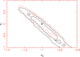
Figure 19: Comparison of $(68\%,95\%)$ likelihood contours deduced using the ‘full methodology’ (Section 2.2; solid lines) and ‘streamlined methodology’ (Section 2.3; dashed lines) for a test survey covering area $4000$ deg² and redshift interval $0.7<z<1.3$. The two sets of contours are in reasonable agreement.

References

- Abdalla & Rawlings (2004) Abdalla, F. & Rawlings, S. 2004, MNRAS, in press (astro-ph/0411342)
- Abraham et al. (2004) Abraham, R. G., et al. 2004, AJ, 127, 2455
- Aldering et al. (2002) Aldering, G., et al. 2002, Proc. SPIE, 4835, 146
- Angulo et al. (2005) Angulo, R., Baugh, C. M., Frenk, C. S., Bower, R. G., Jenkins, A., & Morris, S. L. 2005, MNRAS, submitted (astro-ph/0504456)
- Balbi et al. (2003) Balbi, A., Baccigalupi, C., Perrotta, F., Matarrese, S., & Vittorio, N. 2003, ApJ, 588, L5
- Barden et al. (2004) Barden, S.C., Dey, A., Boyle, B., & Glazebrook, K. 2004, in “Ground-based Instrumentation for Astronomy”, ed. Moorwood and Iye, Proc. SPIE, 5492.
- Bassett & Kunz (2004) Bassett, B. A. & Kunz, M. 2004, ApJ, 607, 661
- Bassett et al. (2005) Bassett, B. A., Parkinson, D., & Nichol R. C. 2005, ApJ, in press (astro-ph/0409266)
- Bernstein (2005) Bernstein, G. 2005, ApJ, submitted (astro-ph/0503276)
- Bolzonella, Miralles, & Pelló (2000) Bolzonella, M., Miralles, J.-M., & Pelló, R. 2000, A&A, 363, 476
- Blake & Glazebrook (2003) Blake, C. & Glazebrook, K. 2003, ApJ, 594, 665
- Blake et al. (2004) Blake, C., Abdalla, F., Bridle, S.L., & Rawlings, S., 2004, New Astron. Rev., 48, 1063
- Blake & Bridle (2005) Blake, C. & Bridle, S.L. 2005, MNRAS, in press (astro-ph/0411713)
- Budavári et al. (2001) Budavári, T., Szalay, A. S., Csabai, I., Connolly, A. J., & Tsvetanov, Z. 2001, AJ, 121, 3266
- Bunton et al. (2003) Bunton, J.D., et al. 2003, “Panorama of the Universe: A Cylindrical Reflector SKA” (see www.skatelescope.org)
- Chen et al. (2003) Chen, H., et al. 2003, ApJ, 586, 745
- Cimatti et al. (2002) Cimatti, A., et al. 2002, A&A, 381, L68
- Cole et al. (2005) Cole, S., et al. 2005, MNRAS, in press (astro-ph/0501174)
- Coles (1993) Coles, P. 1993, MNRAS, 262, 1065
- Collister & Lahav (2004) Collister, A. A. & Lahav, O. 2004, PASP, 116, 345
- Csabai et al. (2000) Csabai, I., Connolly, A. J., Szalay, A. S., & Budavári, T. 2000, AJ, 119, 69
- Davis et al. (2003) Davis, M., et al. 2003, Proc. SPIE, 4834, 161
- de Bernardis et al. (2000) de Bernardis, P., et al. 2000, Nature, 404, 955
- Efstathiou & Bond (1999) Efstathiou, G. & Bond, J. R. 1999, MNRAS, 304, 75
- Eisenstein & Hu (1998) Eisenstein, D. J. & Hu, W. 1998, ApJ, 496, 605
- Eisenstein, Hu, & Tegmark (1999) Eisenstein, D. J., Hu, W., & Tegmark, M. 1999, ApJ, 518, 2
- Eisenstein (2002) Eisenstein D.J., 2002, “Large-scale structure and future surveys” in “Next Generation Wide-Field Multi-Object Spectroscopy”, ASP Conference Series vol. 280, ed. M.Brown & A.Dey (astro-ph/0301623)
- Eisenstein & White (2004) Eisenstein, D., & White, M. 2004, Phys. Rev. D, 70, 103523
- Eisenstein et al. (2005) Eisenstein, D., et al. 2005, ApJ, in press (astro-ph/0501171)
- Feldman, Kaiser, & Peacock (1994) Feldman, H. A., Kaiser, N., & Peacock, J. A. 1994, ApJ, 426, 23
- Fernández-Soto, Lanzetta, & Yahil (1999) Fernández-Soto, A., Lanzetta, K. M., & Yahil, A. 1999, ApJ, 513, 34
- Gallego et al. (1995) Gallego, J., Zamorano, J., Aragon-Salamanca, A., & Rego, M. 1995, ApJ, 455, L1
- Glazebrook et al. (1999) Glazebrook, K., Blake, C., Economou, F., Lilly, S., & Colless, M. 1999, MNRAS, 306, 843
- Glazebrook et al. (2004) Glazebrook, K., Baldry, I., Moos, W., Kruk, J., & McCandliss, S. 2004, New Astronomy Reviews, in press (astro-ph/0410037)
- Hicks et al. (2002) Hicks, E. K. S., Malkan, M. A., Teplitz, H. I., McCarthy, P. J., & Yan, L. 2002, ApJ, 581, 205
- Hopkins, Connolly, & Szalay (2000) Hopkins, A. M., Connolly, A. J., & Szalay, A. S. 2000, AJ, 120, 2843
- Hu & Haiman (2003) Hu, W. & Haiman, Z. 2003, Phys. Rev. D, 68, 063004
- Jansen, Franx & Fabricant (2001) Jansen, R. A., Franx, M., & Fabricant, D. 2001, ApJ, 551, 825
- Le Borgne & Rocca-Volmerange (2002) Le Borgne, D. & Rocca-Volmerange, B. 2002, A&A, 386, 446
- Le Fevre et al. (2003) Le Fevre, O., et al. 2003, Proc. SPIE, 4834, 173
- Lilly et al. (1995) Lilly, S. J., Le Fevre, O., Crampton, D., Hammer, F., & Tresse, L. 1995, ApJ, 455, 50
- Linder (2002) Linder, E. V. 2003, Phys. Rev. Lett., 90, 091301
- Linder (2003) Linder, E. V. 2003, Phys. Rev. D, 68, 083504
- Linder & Jenkins (2003) Linder, E. V. & Jenkins, A. 2003, MNRAS, 346, 573
- Peacock & Dodds (1994) Peacock, J. A. & Dodds, S. J. 1994, MNRAS, 267, 1020
- Perlmutter et al. (1999) Perlmutter, S., et al. 1999, ApJ, 517, 565
- Petro, Kriss & Stockman (2002) Petro, L., Kriss, G., & Stockman, H. S. 2002, STScI Technical Memorandum TM-2002-0004 A
- Pettini et al. (1998) Pettini, M., Kellogg, M., Steidel, C. C., Dickinson, M., Adelberger, K. L., & Giavalisco, M. 1998, ApJ, 508, 539
- Ratra & Peebles (1988) Ratra, B. & Peebles, P. J. E. 1988, Phys. Rev. D, 37, 3406
- Riess et al. (1998) Riess, A. G., et al. 1998, AJ, 116, 1009
- Riess et al. (2004) Riess, A. G., et al. 2004, ApJ, 607, 665
- Scherrer & Weinberg (1998) Scherrer, R. J. & Weinberg, D. H. 1998, ApJ, 504, 607
- Seo & Eisenstein (2003) Seo, H. & Eisenstein, D. J. 2003, ApJ, 598, 720
- Spergel et al. (2003) Spergel, D. N., et al. 2003, ApJS, 148, 175
- Springel et al. (2005) Springel, V., et al. 2005, Nature, in press (astro-ph/0504097)
- Steidel et al. (2003) Steidel, C. C., Adelberger, K. L., Shapley, A. E., Pettini, M., Dickinson, M., & Giavalisco, M. 2003, ApJ, 592, 728
- Steidel et al. (2004) Steidel, C. C., Shapley, A. E., Pettini, M., Adelberger, K. L., Erb, D. K., Reddy, N. A., & Hunt, M. P. 2004, ApJ, 604, 534
- Stover et al. (1998) Stover, R. J., et al. 1998, Proc. SPIE, 3505, 13
- Tegmark (1997) Tegmark, M. 1997, Phys. Rev. Lett., 79, 3806
- Tegmark et al. (2004) Tegmark, M., et al. 2004, Phys. Rev. D, 69, 103501
- Turner et al. (2003) Turner, M. S., et al. 2003, Connecting Quarks with the Cosmos: Eleven Science Questions for the New Century, The National Academies Press, Washington D.C.
- Tyson (2002) Tyson, J. A. 2002, Proc. SPIE, 4836, 10
- Weller & Albrecht (2002) Weller, J. & Albrecht, A. 2002, Phys. Rev. D, 65, 103512
- Wolf et al. (2003) Wolf, C., Meisenheimer, K., Rix, H.-W., Borch, A., Dye, S., & Kleinheinrich, M. 2003, A&A, 401, 73
- Yan et al. (1999) Yan, L., McCarthy, P. J., Freudling, W., Teplitz, H. I., Malumuth, E. M., Weymann, R. J., & Malkan, M. A. 1999, ApJ, 519, L47
- Zwaan et al. (2003) Zwaan, M. A., et al. 2003, AJ, 125, 2842