Stringy Dark Energy Model with Cold Dark Matter

Abstract

Cosmological consequences of adding the Cold Dark Matter (CDM) to the exactly solvable stringy Dark Energy (DE) model are investigated. The model is motivated by the consideration of our Universe as a slowly decaying D3-brane. The decay of this D-brane is described in the String Field Theory framework. Stability conditions of the exact solution with respect to small fluctuations of the initial value of the CDM energy density are found. Solutions with large initial value of the CDM energy density attracted by the exact solution without CDM are constructed numerically. In contrast to the $\Lambda$CDM model the Hubble parameter in the model is not a monotonic function of time. For specific initial data the DE state parameter $w_{DE}$ is also not monotonic function of time. For these cases there are two separate regions of time where $w_{DE}$ being less than $-1$ is close to $-1$.

1 Introduction

Nowadays strings and D-branes found cosmological applications related with the cosmological acceleration [1]-[3]. The combined analysis of the type Ia supernovae, galaxy clusters measurements and WMAP data provides an evidence for the accelerated cosmic expansion [4, 5, 6]. The cosmological acceleration strongly indicates that the present day Universe is dominated by smoothly distributed slowly varying Dark Energy (DE) component (see [7] for reviews), for which the state parameter $w_{DE}$ is negative. Contemporary experiments give strong support that currently the state parameter $w_{DE}$ is close to $-1$, $w_{DE}=-1\pm 0.1$ [6, 8, 9, 10, 11].

From the theoretical point of view the specified domain of $w$ covers three essentially different cases: $w>-1,~{}w=-1$ and $w<-1$ (see [12], and references therein). The most exciting possibility would be the case $w<-1$ corresponding to the so called phantom dominated Universe. In phenomenological models describing this case the weak energy conditions $\varrho>0,\varrho+p>0$ are violated and there are problems with stability at classical and quantum levels [13]. Thus, a phantom becomes a great challenge for the theory while its presence according to the supernovae data is not excluded.

A possible way to evade the stability problem for a phantom model is to yield the phantom as an effective model of a more fundamental theory which has no such problems at all. It has been shown in [3] that such a model does appear in the string theory framework. This DE model assumes that our Universe is a slowly decaying D3-brane which dynamics is described by the tachyonic mode of the string field theory (SFT). The notable feature of the SFT description of the tachyon dynamics is a non-local polynomial interaction [14]-[18]. It turns out the string tachyon behavior is effectively described by a scalar field with a negative kinetic term (phantom) however due to the string theory origin the model is stable at large times.

In [12] we have found an exactly solvable Stringy DE model in the Friedmann Universe. This model is a modified version of the effective SFT model [3] and is inspired by SuperSFT calculations [17]. First level calculations in the SFT give fourth order polynomial interaction. Higher levels increase a power of the interaction. Exactly solvable model has a particular six order polynomial interaction potential. However, small fluctuations of coefficients in that potential do not change the solution qualitatively and one can say that the model [12] represents the behavior of nonBPS D3 brane in the the Friedmann Universe rather well. It is interesting to investigate the dynamics of the model in the presence of the Dark Matter. This is a subject of the present paper.

It turns out from the observational data that DE forms about 73% and the Dark Matter forms about 23% of our Universe. Thus because of a significance of the Dark Matter component in the Universe in the present paper we investigate an interaction of the phantom matter considered in [12] with the CDM. It seems impossible to find exact solutions in the presence of the CDM, except the case when the DE state parameter is a constant [19], so we use numeric methods to analyze the behavior of the phantom field and cosmological parameters in our model.

2 Exactly solvable Phantom Model

We start by recalling the main facts related to the model considered in [12]. This is a model of Einstein gravity interacting with a single phantom scalar field in the spatially flat Friedmann Universe. Since the phantom field comes from the string field theory the string mass $M_{s}$ and a dimensionless open string coupling constant $g_{o}$ emerges. The action is

$$S=\int d^{4}x\sqrt{-g}\left(\frac{M_{P}^{2}}{2M_{s}^{2}}R+\frac{1}{g_{o}^{2}}\left(+\frac{1}{2}g^{\mu\nu}\partial_{\mu}\phi\partial_{\nu}\phi-V(\phi)\right)\right),$$ (1)

where $M_{P}$ is the reduced Planck mass, $g_{\mu\nu}$ is a spatially flat Friedmann metric

$$ds^{2}={}-dt^{2}+a^{2}(t)(dx_{1}^{2}+dx_{2}^{2}+dx_{3}^{2}).$$

and coordinates $(t,x_{i})$ and field $\phi$ are dimensionless. Hereafter we use the dimensionless parameter $m_{p}$ for short:

$$m_{p}^{2}=\frac{g_{o}^{2}M_{P}^{2}}{M_{s}^{2}}.$$ (2)

If the scalar field depends only on time, i.e. $\phi=\phi(t)$, then independent equations of motion are

$$\begin{split}3H^{2}&=\frac{1}{m_{p}^{2}}\>\varrho_{DE},\quad\varrho_{DE}=-\frac{1}{2}\dot{\phi}^{2}+V(\phi),\\ 3H^{2}+2\dot{H}&={}-\frac{1}{m_{p}^{2}}\>p_{DE},\quad p_{DE}=-\frac{1}{2}\dot{\phi}^{2}-V(\phi),\end{split}$$ (3)

Here dot denotes the time derivative, $H\equiv\dot{a}(t)/a(t)$, $\varrho_{DE}$ and $p_{DE}$ are energy and pressure densities of the DE respectively. One can recast the system (3) to the following form

$$\begin{split}\dot{H}&=\frac{1}{2m_{p}^{2}}\dot{\phi}^{2},\\ 3H^{2}&=\frac{1}{m_{p}^{2}}\left(-\frac{1}{2}\dot{\phi}^{2}+V(\phi)\right).\end{split}$$ (4)

Besides of this there is an equation of motion for the field $\phi$ which is in fact a consequence of system (3).

Following the superpotential method [20] (see also [21]) we assume that $H(t)$ is a function (named as superpotential) of $\phi(t)$:

$$H(t)=W(\phi(t)).$$ (5)

This still does not give a systematic way to find general solutions to the system (4) but allows one to construct $W(\phi)$ and $V(\phi)$ for a known function $\phi(t)$. We take for $\phi(t)$

$$\phi(t)=A\tanh(\omega t).$$ (6)

This function is known to describe effectively the late time behavior of the tachyon in the 4-dimensional flat case [22, 23]. The function $\phi(t)$ satisfies the following equation

$$\dot{\phi}=\omega\left(A-\frac{1}{A}\phi^{2}\right).$$

Hence, we obtain

$$W=\frac{\omega}{2m_{p}^{2}}\left(A\phi-\frac{1}{3A}{\phi}^{3}\right),$$ (7)

and corresponding potential

$$V(\phi)=\frac{\omega^{2}}{2A^{2}}\left(A^{2}-\phi^{2}\right)^{2}+\frac{\omega^{2}\phi^{2}}{12A^{2}m_{p}^{2}}\left(3\,A^{2}-\phi^{2}\right)^{2}.$$ (8)

We have omitted an integration constant in (7) to yield an even potential (8). It is typical that to keep the form of solutions to the scalar field equation in the presence of Friedmann metric one has to modify the potential adding a term proportional to the inverse of the reduced Planck mass $M_{P}^{2}$ [12, 24].

The described solution leads to a number of cosmological consequences. The Hubble parameter

$$H=\frac{\omega A^{2}}{2m_{p}^{2}}\tanh(\omega t)\left(1-\frac{1}{3}(\tanh(\omega t))^{2}\right)$$ (9)

goes asymptotically to $\omega A^{2}/(3m_{p}^{2})$ when $t$ goes to infinity. Once $H(t)$ is known one readily obtains the scale factor

$$a(t)=a_{0}(\cosh(\omega t))^{\frac{A^{2}}{3m_{p}^{2}}}\exp\left({\frac{A^{2}(\cosh(\omega t)^{2}-1)}{12m_{p}^{2}\cosh(\omega t)^{2}}}\right),$$ (10)

where $a_{0}$ is an arbitrary constant, and the deceleration parameter

$$q(t)=-\>\frac{\ddot{a}a}{\dot{a}^{2}}={}-1-{\frac{18m_{p}^{2}\left(\cosh(\omega\,t)\right)^{2}}{A^{2}\left(\left(\cosh(\omega\,t)\right)^{2}-1\right)\left(2\,\left(\cosh(\omega\,t)\right)^{2}+1\right)^{2}}}.$$ (11)

It follows from formula (11) that the Universe in this scenario is accelerating.

The expression for the state parameter is the following

$$w_{DE}(\phi)=\frac{p_{DE}(\phi)}{\varrho_{DE}(\phi)}=-1-12m_{p}^{2}\frac{(A^{2}-\phi^{2})^{2}}{\phi^{2}(3A^{2}-\phi^{2})^{2}}.$$ (12)

Point $\phi=A$ corresponds to an infinite future and therefore $w_{DE}\to-1$ as $t\to\infty$.

Plots for the Hubble, deceleration and state parameters are drawn in Fig.1 (Hereafter we assume $A=\omega=1$ for all plots).

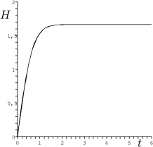
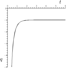
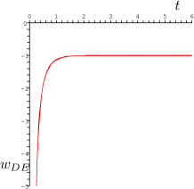
Figure 1: The time evoution of the Hubble parameter $H(t)$ (left), the deceleration parameter $q(t)$ (middle) and the state parameter $w_{DE}(t)$ (right) in the exactly solvable model for $m_{p}^{2}=0.2$.

Thus, we conclude by noting that in our model the phantom field provides the DE dominated accelerating Universe.

3 Interaction with Cold Dark Matter

3.1 The Model

Now we are going to couple in a minimal way a pressureless matter of energy density $\varrho_{M}$ (the CDM) to our model such that the Friedmann equations get an extra term

$$3H^{2} = \frac{1}{m_{p}^{2}}\left(-\frac{1}{2}\dot{\phi}^{2}+V(\phi)+\varrho_{M}(a)\right),$$ (13)

$$\dot{H} = \frac{1}{2m_{p}^{2}}\left(\dot{\phi}^{2}-\varrho_{M}(a)\right).$$ (14)

and the equation describing the evolution of scalar field has previous form

$$\ddot{\phi}+3H\dot{\phi}-V_{\phi}^{\prime}=0.$$ (15)

From (13)–(15) we obtain the conservation of the energy density for the CDM:

$$\dot{\varrho}_{M}+3H\varrho_{M}=0,$$ (16)

that after integration gives

$$\varrho_{M}=\varrho_{M,0}e^{-3\int\limits^{t}H(\tau)d\tau}=\varrho_{M,0}\left(\frac{a}{a_{0}}\right)^{-3},$$ (17)

where constants $\varrho_{M,0}$ and $a_{0}$ are initial values of $\varrho_{M}$ and $a$ correspondingly. From (17) we obtain equation (13) in the following form:

$$3H^{2}=\frac{1}{m_{p}^{2}}\left(V(\phi)-\frac{~{}\dot{\phi}^{2}}{2}+\varrho_{M,0}\left(\frac{a_{0}}{a}\right)^{3}\right).$$ (18)

Following the lines of [12] we address to our analysis the questions of cosmological evolution and stability.

The straightforward way to study a stability of solutions to the system of equations (13)–(15) is to exclude $\varrho_{M}$ from (13),(14) and obtain the following system:

$$\ddot{\phi} + 3H\dot{\phi}-V_{\phi}^{\prime}=0,$$ (19)

$$2\dot{H}+3H^{2} = \frac{1}{m_{p}^{2}}\left(\frac{1}{2}\dot{\phi}^{2}+V(\phi)\right).$$ (20)

Depending on the initial values of $H$, $\phi$ and $\dot{\phi}$, which have been considered as independent, this system describes our model either with or without the CDM. In particular, the initial values: $H_{0}=0$, $\phi_{0}=0$ and $\dot{\phi}_{0}=A\omega$ correspond to the exact solution (6).

Either one can perform calculations using nonautonomous system of equations [25] which can be obtained from equations (15) and (18) in the following form

$$\frac{d\phi}{dn} = \frac{1}{H(\phi,\psi,n)}~{}\psi,$$ (21)

$$\frac{d\psi}{dn} = {}-3\psi+\frac{1}{H(\phi,\psi,n)}~{}\frac{dV(\phi)}{d\phi},$$ (22)

where

$$H(\phi,\psi,n)=\frac{1}{\sqrt{3}M_{p}}\sqrt{-\frac{1}{2}\psi^{2}+V(\phi)+\varrho_{M,0}e^{-3n}},~{}\dot{\phi}=\psi~{}\text{and}~{}n=\ln(a/a_{0}).$$

3.2 Stability analysis for small fluctuations.

In [12] we have analyzed the system (13)–(15) without the CDM under condition $A=\omega=1$ and found that the exact solution $\phi=\tanh(t)$ is stable with respect to small fluctuations of the initial conditions if and only if $m_{p}^{2}\leqslant 1/2$.

Let us consider the behavior of the solution of system (19)–(20) in the neighborhood of the exact solution

$$\begin{split}\phi_{0}(t)&=\tanh(t),\\ \dot{\phi}_{0}(t)&\equiv\psi_{0}(t)=1-\tanh(t)^{2},\\ H_{0}(t)&=\frac{1}{2m_{p}^{2}}\tanh(t)\left(1-\frac{1}{3}\tanh(t)^{2}\right).\end{split}$$

Substituting

$$H(t)=H_{0}(t)+\varepsilon H_{1}(t),\quad\phi(t)=\phi_{0}(t)+\varepsilon\phi_{1}(t)\quad\mbox{and}\quad\dot{\phi}(t)\equiv\psi(t)=\psi_{0}(t)+\varepsilon\psi_{1}(t),$$ (23)

in (19) and (20) we obtain in the first order of $\varepsilon$ the following equations:

$$\begin{array}[]{@{}rcl@{}}\displaystyle\dot{\phi}_{1}&\displaystyle=&\displaystyle\psi_{1},\\[10.5275pt] \displaystyle\dot{\psi}_{1}&\displaystyle=&\displaystyle\frac{1}{m_{p}^{2}}\left(2(2m_{p}^{2}-1)-\frac{6m_{p}^{2}-1}{\cosh(t)^{2}}\right)\phi_{1}-{}\\[7.68222pt] &\displaystyle-&\displaystyle\frac{(2\cosh(t)^{2}+1)\tanh(t)}{2m_{p}^{2}\cosh(t)^{2}}\psi_{1}-\frac{3}{\cosh(t)^{2}}H_{1},\\[10.5275pt] \displaystyle\dot{H}_{1}&\displaystyle=&\displaystyle\frac{\tanh(t)}{4m_{p}^{2}\cosh(t)^{4}}\displaystyle\left(1+(2-4m_{p}^{2})\cosh(t)^{2}\right)\phi_{1}+{}\\[7.68222pt] &\displaystyle+&\displaystyle\frac{1}{2\cosh(t)^{2}}\psi_{1}-\frac{(1+2\cosh(t)^{2})\tanh(t)}{2\cosh(t)^{2}}H_{1}.\\ \end{array}$$ (24)

System (24) has been solved with the help of the computer algebra system Maple. The exact dependence $\phi_{1}(t)$, $\psi_{1}(t)$ and $H(t)$ are too cumbersome to be presented here. The main result is that for $m_{p}^{2}\leqslant 1/2$ functions $\phi_{1}(t)$, $\psi_{1}(t)$ and $H_{1}(t)$ are bounded functions and our exact solution is stable.

Note that numerical calculations show that if $m_{p}^{2}\leqslant 1/2$ then even for large initial values of the CDM energy density numerical solutions tend to the exact solution as $t$ tends to infinity.

3.3 Numeric solutions. Time dependence.

At this point we pass to numeric methods because it seems impossible to find exact solutions in the presence of the CDM. To analyze the cosmological evolution it is instructive to plot phase curves for the scalar field as well as evolution of the state parameter $w_{DE}$ for the scalar matter. In addition we find numerically a ratio of the energy densities for the CDM and the DE. Experimental bounds for this ratio is known and estimated to be near $1/3$ so we can find the time point we live and a corresponding value of $w_{DE}$ in our approach.

Due to equation (18) initial data $\phi_{0},~{}\dot{\phi}_{0}$ and $H_{0}$ do fix an initial value of the CDM density. To have a given initial energy density of the CDM we take $\phi_{0}$ and $\dot{\phi}_{0}$ and find the corresponding value $H_{0}$. In particular, to have $\varrho_{M,0}=1$, $\phi_{0}=0$, $\dot{\phi}_{0}=1$ for $m_{p}^{2}=0.2$ we must take $H_{0}=\sqrt{5/3}\approx 1.29$. For this initial values numeric solutions are presented graphically in Fig.2.

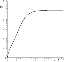
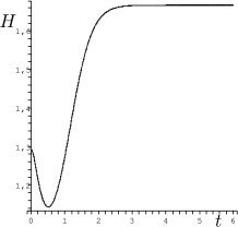
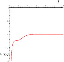
Figure 2: The time evolution of the scalar field $\phi(t)$, the Hubble parameter $H(t)$ and the state parameter $w_{DE}(t)$. $\varrho_{M,0}=1$, $m_{p}^{2}=0.2$ and $\dot{\phi}_{0}=1$.

In Fig.3 we present the same plots for $\varrho_{M,0}=100$. Corresponding $H_{0}=10\sqrt{5/3}$.

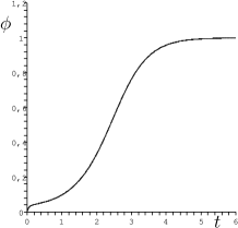
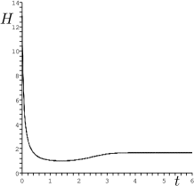
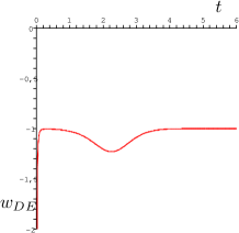
Figure 3: The time evolution of the scalar field $\phi(t)$, the Hubble parameter $H(t)$ and the state parameter $w_{DE}(t)$. $\varrho_{M,0}=100$, $m_{p}^{2}=0.2$ and $\dot{\phi}_{0}=1$.

Comparing Figs.2 and 3 with Fig.1 one can see that our solutions with and without the CDM are different only in the beginning of the evolution where the CDM dominates (if exists). Note, that the behavior of the Hubble parameter in the presence of the CDM is not monotonic and the DE state parameter may be not monotonic as well.

3.4 Numeric solutions. $\phi$-dependence.

It turns out that values of the $w_{DE}$ as well as ratio $\varrho_{CDM}/\varrho_{DE}$ which are observational cosmological parameters [6, 9, 11] can be found easier using equations (21), (22) as functions of the e-folding number $n$. However, it is more instructive to find a dependence on $\phi$ and not on $n$.

Let us recall that from an analysis of our phantom model without the CDM we know that the scalar field interpolates between an unstable and a nonperturbative vacua during infinite time similar to the non-BPS string tachyon [22, 23]. In our notations nonperturbative vacuum corresponds to $\phi=+1$. In the pure phantom model the evolution is described by $\phi(t)=A\tanh(\omega t)$ function, where $A$ and $\omega$ can be rescaled to 1. This dependence is monotonic and this allows us to find physical variables as functions of $\phi$.

The situation is more complicated in the presence of the CDM. First, we do not know an exact time dependence of the scalar field. Second, it is not evident for arbitrary initial data and value of parameter $m_{p}^{2}$ that the scalar field evolves monotonically. However, in the particular cases presented in Figs. 2 and 3 our solutions $\phi(t)$ are monotonic functions of time and moreover look like $\tanh(t)$ at large times. Below we are interesting in solutions which approach the nonperturbative vacuum during an infinite time. Thus, the point $\phi=1$ corresponds to an infinite future. The $\phi(t)$ dependence can be found numerically to pass from $\phi$ coordinate to the time.

In Figs.4–6 we plot results of numeric solutions to equations (21), (22) that allow us to find physical variables such as $H$, $w_{DE}$, $\varrho_{CDM}/\varrho_{DE}$ as function of the field $\phi$.

$~{}~{}~{}~{}~{}~{}~{}~{}\rho_{M,0}=0.01,~{}~{}~{}~{}~{}~{}~{}~{}~{}~{}~{}~{}~{}~{}~{}~{}~{}~{}~{}\rho_{M,0}=1~{}~{}~{}~{}~{}~{}~{}~{}~{}~{}~{}~{}~{}~{}~{}~{}~{}~{}~{}~{}~{}\rho_{M,0}=100$
 
 

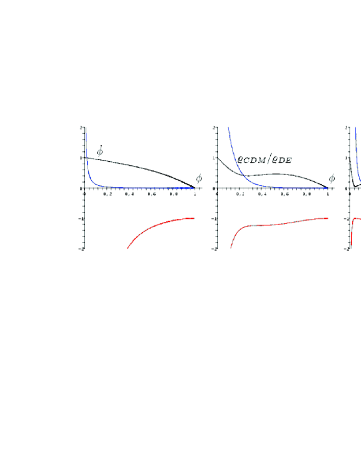
Figure 4: $\phi$-dependence of the velocity $\dot{\phi}$ (black line), the state parameter $w_{DE}$ (red line) and the $\varrho_{CDM}/\varrho_{DE}$ ratio (blue line). Initial velocity of the scalar field is equal to $1$ and $m_{p}^{2}=0.2$.

$m_{p}^{2}=0.2,~{}\rho_{M,0}=0.01~{}~{}~{}~{}~{}~{}m_{p}^{2}=0.2,~{}\rho_{M,0}=1~{}~{}~{}~{}~{}~{}m_{p}^{2}=0.2,~{}\rho_{M,0}=100$
 
 

 
 
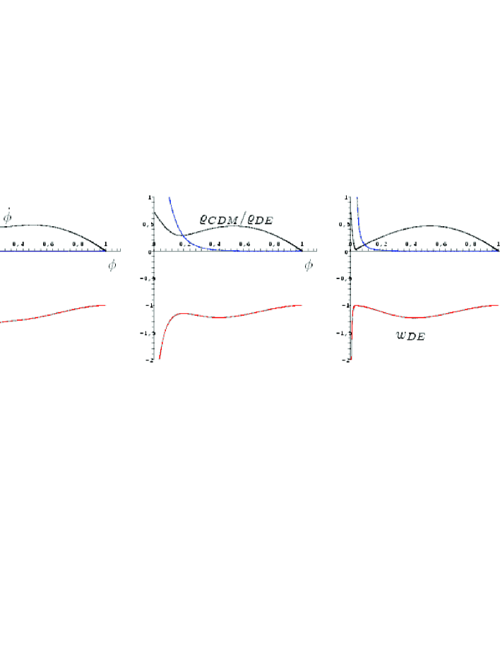
$m_{p}^{2}=0.6,~{}\rho_{M,0}=0.01~{}~{}~{}~{}~{}~{}m_{p}^{2}=1,~{}\rho_{M,0}=0.01~{}~{}~{}~{}~{}~{}m_{p}^{2}=1,~{}\rho_{M,0}=1$
 
 

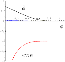
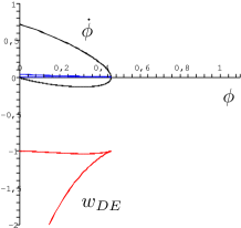
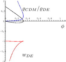
Figure 5: $\phi$-dependence of the velocity $\dot{\phi}$ (black line), the state parameter $w_{DE}$ (red line) and the $\varrho_{CDM}/\varrho_{DE}$ ratio (blue line). Initial velocity of the scalar field is equal to $0.72$.

$~{}~{}~{}~{}~{}~{}~{}~{}m_{p}^{2}=0.2,~{}~{}~{}~{}~{}~{}~{}~{}~{}~{}~{}~{}~{}~{}~{}~{}~{}~{}~{}m_{p}^{2}=0.6~{}~{}~{}~{}~{}~{}~{}~{}~{}~{}~{}~{}~{}~{}~{}~{}~{}~{}~{}m_{p}^{2}=1$
 

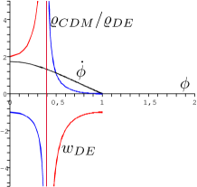
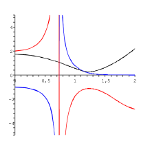
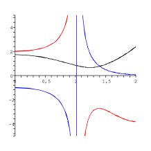
Figure 6: $\phi$-dependence of the velocity $\dot{\phi}$ (black line), the state parameter $w_{DE}$ (red line) and the $\varrho_{CDM}/\varrho_{DE}$ ratio (blue line). Initial velocity of the scalar field is equal to its maximal possible value.

These sets of plots differ in an initial velocity of the scalar field. Note that it follows from (18) that there exists a maximal initial velocity $\psi_{0m}$ for our phantom field. $\psi_{0m}$ depends on values of $\phi_{0}$, $\varrho_{M,0}$ and $a_{0}$ and does not depend on $m^{2}_{p}$. In all plots $a_{0}=1$ and $\phi_{0}=0$ . All plots have three curves: black ones are phase curves, red ones are $w$-s and blue ones are $\varrho_{CDM}/\varrho_{DE}$ ratios. In Fig. 4 the initial velocity is equal to $1$ (which is the same as for the exact solution), $m_{p}^{2}=0.2$ and $\varrho_{M,0}$ is equal to $0.01$, $1$ and $100$ from left to right. Here we see that the scalar field reaches $+1$. This indicates a stability of the system with respect to fluctuations of the initial CDM energy density for small $m_{p}^{2}$. In Fig.5 the initial velocity is equal to $0.72$. The first row there corresponds to $m_{p}^{2}=0.2$ and $\varrho_{M,0}$ is equal to $0.01$, $1$ and $100$ from left to right. The second row shows the behavior of the system with $m_{p}^{2}$ equal to $0.6$ and $1$ and $\varrho_{M,0}$ equal to $0.01$ and with $m_{p}^{2}$ equal to $1$ and $\varrho_{M,0}$ equal to $1$. One again sees from these plots that the scalar field reaches $1$ for small values of $m_{p}^{2}$ in a wide range of an initial CDM energy density.

This situation is broken for greater $m_{p}^{2}$ even for a small initial CDM energy density and the field does not reach $1$. In Fig. 6 $\varrho_{M,0}$ is taken to be $1$, the initial velocity is equal to its maximal possible value $\psi_{0m}$ and $m_{p}^{2}$ is equal to $0.2$, $0.6$ and $1$ from left to right. Here we again observe a stability for small $m_{p}$ and also find out that for large $m_{p}^{2}$ the scalar field goes beyond the point $1$. Also for the maximal possible initial velocities $w_{DE}$ and $\varrho_{CDM}/\varrho_{DE}$ functions have a discontinuity. One can understand this qualitatively because the energy density for the DE has two terms with opposite signs. Indeed, the scalar field is a phantom and its kinetic energy is negative while the potential term is positive. Thus at some point the energy density of the DE changes the sign and develops a discontinuity in $w_{DE}$ and $\varrho_{CDM}/\varrho_{DE}$ ratio. Such a behavior is rather undesirable from cosmological point of view, since the is no observational data indicated singular behavior of cosmological parameters and we do not consider corresponding plots further.

Hence, seeking for a situation where field $\phi$ approaches $1$ and there is no cosmological singularities during this evolution we are left with the first row in Fig. 4 and Fig. 5. In this plots phase curves show that field $\phi$ indeed depends monotonically on time because $\dot{\phi}$ is always positive during the evolution. Looking for specified plots we draw the reader’s attention to the following interesting properties of our model. First, $\varrho_{CDM}/\varrho_{DE}$ ratio dependence is monotonic and experimentally measured value $1/3$ is close to the beginning of the evolution. For example, in Fig. 4 (left) this point corresponds to $w_{DE}\approx-1.02$ and $\phi\approx 0.09$. Moreover, this is not a distinguished value and it follows from the model that this ratio will decrease with time. Second, for $\rho_{M,0}$ large enough $w_{DE}$ behaves non-monotonically.

4 Discussion and Conclusion

To summarize, let us also note that we get an existence of a region of the initial energy density of the CDM, for which $w_{DE}$ is not monotonic. Such a behavior is interesting and very surprising. We see that for large initial energy densities of the CDM $w_{DE}$ grows with time from minus infinity to approximately $-1$, then goes down to a local minimum and after this grows again asymptotically approaching $-1$. Note, that it has been proved in [26] that under some (compare with [27]) conditions the phantom matter cannot cross the $w=-1$ barrier. For small initial energy densities of the CDM we cannot say that $w_{DE}$ has a local minimum but its rate of change becomes slower and faster. We especially point out that the very first time stamp when $w_{DE}$ approaches $-1$ (or its rate of change decreases essentially) is approximately the same where $\varrho_{CDM}/\varrho_{DE}$ ratio is close to $1/3$. It is worth to note that juxtaposing Figures 2–3 and Figures 4–6 we see that the present ratio of the CDM and the DE energy densities also corresponds to a local minimum of the Hubble parameter.

It is interesting to find an influence of the higher open string mass levels as well as an influence of the closed string excitations on the obtained picture. Even in the flat space-time the dynamics of a D-brane change drastically when the closed string excitations are included [28, 29].

We get a stable behavior and smooth cosmological parameters in the stringy inspired model only in the case when the dimensionless parameter $m^{2}_{p}$ is less than $0.5$. This restricts the parameters of the original theory [3] the model considered in this paper comes from. Let us recall that $m^{2}_{p}$ is related with the reduced Planck mass, the string mass parameter $M_{s}^{2}$ and the open string coupling constant $g_{o}^{2}$:

$$m^{2}_{p}=\frac{g_{o}^{2}M^{2}_{P}}{M^{2}_{s}}$$

Therefore, to have an acceptable cosmological solution we have to assume that $2g_{o}^{2}M^{2}_{P}<M^{2}_{s}$. Here $M_{P}$ is the 4-dimensional Planck mass. The effective string mass depends on the 10-dimensional mass parameter $1/l_{s}$, where $l_{s}$ is a string length and the compactification volume $V_{6}$. Taking into account that $M^{2}_{s}\sim V_{6}/l^{8}_{s}$ and using the usual requirement that $l_{s}\sim 1/M_{P}$ we get

$$m^{2}_{p}=\frac{g_{o}^{2}M^{2}_{P}}{M^{2}_{s}}\sim\frac{g_{o}^{2}M^{2}_{P}l^{8}_{s}}{V_{6}}\sim\frac{g_{o}^{2}l^{6}_{s}}{V_{6}}<0.5,$$

that looks reasonable from a general point of view.

References

- [1] A. Sen, JHEP 0204, 048 (2002), Rolling Tachyon, hep-th/0203211; A. Sen, JHEP 0207, 065 (2002), Tachyon Matter, hep-th/0203265; A. V. Frolov, L. Kofman, A.A. Starobinsky, Prospects and problems of tachyon matter cosmology, Phys.Lett. B545 (2002) 8–16, hep-th/0204187; G. N. Felder, L. Kofman, A. Starobinsky, Caustics in tachyon matter and other Born-Infeld scalars. JHEP 0209 (2002) 026, hep-th/0208019; G.W. Gibbons, Thoughts on Tachyon Cosmology, Class.Quant.Grav. 20 (2003) S321–S346, hep-th/0301117. A. Sen, Tachyon Dynamics in Open String Theory, hep-th/0410103.
- [2] C. Deffayet, G. Dvali, G. Gabadadze, Accelerated Universe from Gravity Leaking to Extra Dimensions, Phys. Rev. D65 (2002) 044023, astro-ph/0105068 R. Kallosh and A.Linde, M-theory, Cosmological Constant and Anthropic Principle, Phys.Rev. D67 (2003) 023510, hep-th/0208157 Sh. Mukohyama and L. Randall, A dynamical approach to the cosmological constant, Phys.Rev.Lett. 92 (2004) 211302, hep-th/0306108 V. Sahni, Y. Shtanov, Brane World Models of Dark Energy, JCAP 0311 (2003) 014, astro-ph/0202346; Ph. Brax, C. van de Bruck and A.-C. Davis, Brane world cosmology, Rept.Prog.Phys. 67 (2004) 2183–2232, hep-th/0404011; Th.N. Tomaras, Brane-world evolution with brane-bulk energy exchange, hep-th/0404142; E.J. Copeland, M.R. Garousi, M. Sami, Sh. Tsujikawa, What is needed of a tachyon if it is to be the dark energy?, hep-th/0411192; B. McInnes, The phantom divide in string gas cosmology, Nucl.Phys. B718 (2005) 55–82, hep-th/0502209; G. Calcagni, Sh. Tsujikawa, and M. Sami, Dark energy and cosmological solutions in second-order string gravity, hep-th/0505193
- [3] I.Ya. Aref’eva, Nonlocal String Tachyon as a Model for Cosmological Dark Energy, astro-ph/0410443.
- [4] A. G. Riess et al., Observational Evidence from Supernovae for an Accelerating Universe and a Cosmological Constant, Astron. J. 116 (1998) 1009–1038, astro-ph/9805201.
- [5] S.J. Perlmutter et al., Measurements of Omega and Lambda from 42 High-Redshift Supernovae, Astroph. J. 517 (1999) 565, astro-ph/9812133.
- [6] D.N. Spergel et al., First Year Wilkinson Microwave Anisotropy Probe (WMAP) Observations: Determination of Cosmological Parameters, Astroph. J. Suppl. 148 (2003) 175, astro-ph/0302209.
- [7] V. Sahni, Dark Matter and Dark Energy, astro-ph/0403324. P. Frampton, Dark energy — a pedagogic review, astro-ph/0409166. T. Padmanabhan, Cosmological Constant — the Weight of the Vacuum, Phys. Rept. 380 (2003) 235–320, hep-th/0212290.
- [8] J.L. Tonry et al., Cosmological Results from High-z Supernovae, Astrophys. J. 594 (2003) 1–24, astro-ph/0305008.
- [9] M.Tegmark at al., Cosmological parameters from SDSS and WMAP, Phys. Rev. D69 (2004) 103501, astro-ph/0310723; M.Tegmark, What does inflation really predict?, JCAP 0504 (2005) 001, astro-ph/0410281
- [10] A. G. Riess et al., Type Ia Supernova Discoveries at From the Hubble Space Telescope: Evidence for Past Deceleration and Constraints on Dark Energy Evolution, Astrophys.J. 607 (2004) 665–687, astro-ph/0402512
- [11] U.Seljak at al., Cosmological parameter analysis including SDSS Ly-alpha forest and galaxy bias: constraints on the primordial spectrum of fluctuations, neutrino mass, and dark energy, aspto-ph/0407372
- [12] I.Ya. Aref’eva, A.S. Koshelev, S.Yu. Vernov, Exactly solvable SFT insipred phantom model, astro-ph/0412619.
- [13] R.R. Caldwell, Dark Energy, Physics World, 17, No. 5 (2004) 37. R.R. Caldwell, A Phantom Menace? Cosmological consequences of a dark energy component with super-negative equation of state, Phys. Lett. B545 (2002) 23, astro-ph/9908168. R.R. Caldwell, M. Kamionkowski, N.N. Weinberg, Phantom Energy and Cosmic Doomsday, Phys. Rev. Lett. 91 (2003) 071301, astro-ph/0302506 B. McInnes, The dS/CFT Correspondence and the Big Smash, JHEP 0208 (2002) 029, hep-th/0112066. S. Nesseris, L. Perivolaropoulos, The Fate of Bound Systems in Phantom and Quintessence Cosmologies, Phys. Rev. D70 (2004) 123529, astro-ph/0410309 S.M. Carroll, M. Hoffman, M. Trodden, Can the dark energy equation-of-state parameter be less than -1?, Phys. Rev. D68 (2003) 023509, astro-ph/0301273. J.M. Cline, S. Jeon, G.D. Moore, The phantom menaced: constraints on low-energy effective ghosts, Phys. Rev. D70 (2004) 043543, hep-ph/0311312. S.D.H. Hsu, A. Jenkins, M.B. Wise, Gradient instability for , Phys. Lett. B597 (2004) 270–274, astro-ph/0406043. V.K. Onemli, R.P. Woodard, Super-Acceleration from Massless, Minimally Coupled , Class. Quant. Grav. 19 (2002) 4607, gr-qc/0204065; V.K. Onemli, R.P. Woodard, Quantum effects can render on cosmological scales, Phys. Rev. D70 (2004) 107301, gr-qc/0406098. U. Alam, V. Sahni, A.A. Starobinsky, The case for dynamical dark energy revisited, JCAP 0406 (2004) 008, astro-ph/0403687. T. Padmanabhan, Accelerated expansion of the universe driven by tachyonic matter, Phys. Rev. D66 (2002) 021301, hep-th/0204150; T. Padmanabhan, T. Roy Choudhury, Can the clustered dark matter and the smooth dark energy arise from the same scalar field ?, Phys.Rev. D66 (2002) 081301, hep-th/0205055. A. Melchiorri, L. Mersini, C.J. Odman, M. Trodden, The State of the Dark Energy Equation of State, Phys. Rev. D68 (2003) 043509, astro-ph/0211522. Bo Feng, Xiulian Wang, Xinmin Zhang, Dark Energy Constraints from the Cosmic Age and Supernova, astro-ph/0404224; Bo Feng, Mingzhe Li, Yun-Song Piao, Xinmin Zhang, Oscillating Quintom and the Recurrent Universe, astro-ph/0407432. S. Nojiri, S. Odintsov, The final state and thermodynamics of dark energy universe, hep-th/0408170. W. Fang, H.Q. Lu, Z.G. Huang, K.F. Zhang, Phantom Cosmology with Born-Infeld Type Scalar Field, hep-th/0409080. Jian-gang Hao, Xin-zhou Li, Attractor Solution of Phantom Field, Phys. Rev. D67 (2003) 107303, gr-qc/0302100. P. Singh, M. Sami, N. Dadhich, Cosmological Dynamics of Phantom Field, Phys. Rev. D68 (2003) 023522, hep-th/0305110. Rong-Gen Cai, Anzhong Wang, Cosmology with Interaction between Phantom Dark Energy and Dark Matter and the Coincidence Problem, hep-th/0411025. Zong-Kuan Guo, Yuan-Zhong Zhang, Interacting Phantom Energy, astro-ph/0411524. S.M. Carroll, A. De Felice, M. Trodden, Can we be tricked into thinking that is less than -1?, astro-ph/0408081.
- [14] E. Witten, Noncommutative geometry and string field theory, Nucl. Phys. B268 (1986) 253; E. Witten, Interacting field theory of open superstrings, Nucl.Phys. B276 (1986) 291.
- [15] I.Ya. Aref’eva, P.B. Medvedev and A.P. Zubarev, Background formalism for superstring field theory, Phys.Lett. B240 (1990) 356; C.R. Preitschopf, C.B. Thorn and S.A. Yost, Superstring Field Theory, Nucl.Phys. B337 (1990) 363; I.Ya. Aref’eva, P.B. Medvedev and A.P. Zubarev, New representation for string field solves the consistency problem for open superstring field, Nucl.Phys. B341 (1990) 464;
- [16] N. Berkovits, A. Sen and B. Zwiebach, Tachyon Condensation in Superstring Field Theory, Nucl.Phys. B587 (2000) 147-178, hep-th/0002211.
- [17] I.Ya. Arefeva, D.M. Belov, A.S. Koshelev, P.B. Medvedev, Tahyon Condensation in the Cubic Superstring Field Theory, Nucl.Phys B638 ( 2002) 3–20, hep-th/0011117; Gauge Invariance and Tahyon Condensation in the Cubic Superstring Field Theory, Nucl.Phys B638 (2002) 21–40, hep-th/0107197.
- [18] K. Ohmori, A Review on Tachyon Condensation in Open String Field Theories, hep-th/0102085; I.Ya. Aref’eva, D.M. Belov, A.A. Giryavets, A.S. Koshelev, P.B. Medvedev, Noncommutative Field Theories and (Super)String Field Theories, hep-th/0111208; W.Taylor, Lectures on D-branes, tachyon condensation and string field theory, hep-th/0301094.
- [19] V. Sahni, A.A. Starobinsky, The Case for a Positive Cosmological Lambda-term, Int. J. Mod. Phys. D9 (2000) 373, astro-ph/9904398.
- [20] O. DeWolfe, D.Z. Freedman, S.S. Gubser, A. Karch, Modeling the fifth dimension with scalars and gravity, Phys. Rev. D62 (2000) 046008, hep-th/9909134.
- [21] T. Padmanabhan, Accelerated expansion of the universe driven by tachyonic matter, Phys.Rev. D66 (2002) 021301, hep-th/0204150
- [22] I.Ya. Aref’eva, L.V. Joukovskaya, A.S. Koshelev, Time Evolution in Superstring Field Theory on non-BPS brane. Rolling Tachyon and Energy-Momentum Conservation, hep-th/0301137. I.Ya. Aref’eva, Rolling tachyon in NS string field theory, Fortschr. Phys., 51 (2003) 652; I.Ya. Aref’eva and L.V. Joukovskaya, Rolling Tachyon on non-BPS brane, Lectures given at the II Summer School in Modern Mathematical Physics, Kopaonik, Serbia, 1-12 Sept. 2002.
- [23] Ya.I. Volovich, Numerical study of Nonlinear Equations with Infinite Number of Derivatives, J.Phys. A36 (2003) 8685–8702, math-ph/0301028; V.S. Vladimirov and Ya.I. Volovich, Nonlinear Dynamics Equation in p-Adic String Theory, Theor. Math. Phys., 138 (2004) 297–309, math-ph/0306018
- [24] I.Ya. Aref’eva, L.V. Joukovskaya, Time Lumps in Nonlocal Stringy Models and Cosmological Applications, hep-th/0504200.
- [25] C. Armendariz-Picon, V. Mukhanov, Paul J. Steinhardt, Essentials of k-essence, Phys.Rev. D63 (2001) 103510, astro-ph/0006373
- [26] A. Vikman, Can dark energy evolve to the Phantom?, Phys. Rev. D71, 023515 (2005), astro-ph/0407107;
- [27] A.A. Andrianov, F. Cannata, and A.Y. Kamenshchik, Smooth dynamical (de)-phantomization of a scalar field in simple cosmological models, gr-qc/0505087.
- [28] K. Ohmori, Toward Open-Closed String Theoretical Description of Rolling Tachyon, Phys.Rev. D69 (2004) 026008.
- [29] L. Joukovskaya and Ya. Volovich, Energy Flow from Open to Closed Strings in a Toy Model of Rolling Tachyon, math-ph/0308034.