Rates and Progenitors of Type Ia Supernovae

Abstract

The remarkable uniformity of Type Ia supernovae has allowed astronomers to use them as distance indicators to measure the properties and expansion history of the Universe. However, Type Ia supernovae exhibit intrinsic variation in both their spectra and observed brightness. The brightness variations have been approximately corrected by various methods, but there remain intrinsic variations that limit the statistical power of current and future observations of distant supernovae for cosmological purposes. There may be systematic effects in this residual variation that evolve with redshift and thus limit the cosmological power of SN Ia luminosity-distance experiments.

To reduce these systematic uncertainties, we need a deeper understanding of the observed variations in Type Ia supernovae. Toward this end, the Nearby Supernova Factory has been designed to discover hundreds of Type Ia supernovae in a systematic and automated fashion and study them in detail. This project will observe these supernovae spectrophotometrically to provide the homogeneous high-quality data set necessary to improve the understanding and calibration of these vital cosmological yardsticks.

From 1998 to 2003, in collaboration with the Near-Earth Asteroid Tracking group at the Jet Propulsion Laboratory, a systematic and automated searching program was conceived and executed using the computing facilities at Lawrence Berkeley National Laboratory and the National Energy Research Supercomputing Center. An automated search had never been attempted on this scale. A number of planned future large supernovae projects are predicated on the ability to find supernovae quickly, reliably, and efficiently in large datasets.

A prototype run of the SNfactory search pipeline conducted from 2002 to 2003 discovered 83 SNe at a final rate of 12 SNe/month. A large, homogeneous search of this scale offers an excellent opportunity to measure the rate of Type Ia supernovae. This thesis presents a new method for analyzing the true sensitivity of a multi-epoch supernova search and finds a Type Ia supernova rate from $z\sim 0.01$–$0.1$ of $r_{V}=3.67\ _{-1.66}^{+1.20}\mathrm{(stat)}\ _{-0.11}^{+0.11}\mathrm{(sys)}~{}h^{3}\times 10^{-4}$ SNe Ia/yr/Mpc³ from a preliminary analysis of a subsample of the SNfactory prototype search.

Several unusual supernovae were found in the course of the SNfactory prototype search. One in particular, SN 2002ic, was the first SN Ia to exhibit convincing evidence for a circumstellar medium and offers valuable insight into the progenitors of Type Ia supernovae.

Part I Background and Context

Chapter 0 Cosmology with Type Ia Supernovae

Cosmology was revolutionized at the end of the 20th century by the remarkable discovery that the expansion of the Universe is accelerating. This completely unexpected result sparked a flurry of theoretical and experimental activity to understand and better describe this surprising behavior. Type Ia supernovae (SNe Ia) were at the heart of this discovery.

The usefulness of SNe Ia as cosmological probes extends from the evolution and history of the dynamics of the Universe to the formation of the galaxies and stars within. Serving as cosmological beacons, SNe Ia provide reference points in the cosmic fabric through the characteristic brightness of their explosions. Their unique nature makes studies of SN Ia progenitors vital to understanding stellar formation and death. Measurements of the rate of supernovae as a function of redshift provide valuable clues to star formation in and evolution of galactic populations.

While this dissertation focuses on the rates and progenitors of SNe Ia, the work presented here was done in the context of improving the cosmological utility of SNe Ia. Thus, this introduction begins with a survey of SNe Ia and concludes with an overview of how SNe Ia can be used to study the expansion history of the Universe and a discussion of the improvements in our understanding of SNe Ia that are necessary for elucidating the mysteries of dark energy.

1 Type Ia Supernovae

1 Classification of Supernovae

Supernovae are classified based on their observed spectral features and light-curve behavior. The spectrum of a supernova contains a wealth of information about the composition of and distribution of elements in the exploding star. The characteristic broad features of supernovae reflect the spread in velocities inherent in an expanding atmosphere and are key in confirming that a new object is indeed a supernova. The individual elemental lines provide information about the progenitor system and the new elements created in the explosion. The phenomenological definition of supernova types derives from spectral features such as hydrogen emission and silicon absorption.

Supernovae lacking hydrogen absorption or emission lines are classified as Type I supernovae while supernovae with hydrogen lines are classified as Type II supernovae. The Type I supernovae are further divided into Type Ia, Type Ib, and Type Ic, depending on the presence or absence of silicon and helium features (Hillebrandt & Niemeyer 2000). Type Ia supernovae show a clear silicon absorption line at 6700 Å while Type Ib supernovae show evidence of helium lines. Type Ic supernovae show no traces of silicon or helium, but their spectra resemble that of Type Ib at late times. Type II supernovae are commonly divided into four sub-types. SNe IIb supernovae are observationally similar to SNe Ib, but show evidence for a thin hydrogen envelope at early times. SNe IIL have light curves with a steep “Linear” decline, SNe IIn exhibit “narrow” spectroscopic lines, and SNe IIP decline slowly with a long “Plateau” phase after maximum-light. See Fig. 1 for a diagram of the different supernova classifications.

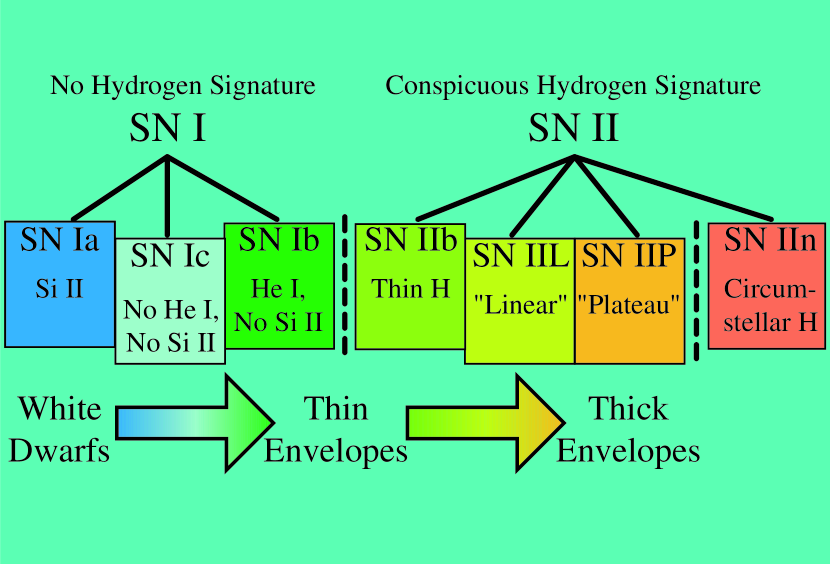
Figure 1: Classification of supernova types. Type I supernovae exhibit no sign of hydrogen in their spectra while Type II do exhibit hydrogen. Type I supernovae are further sub-classified by other spectral features while Type II supernovae are further sub-classified by the shape of their light curves (IIL, IIP) and their spectroscopic features (IIn). Type Ia supernovae show the spectroscopic signatures of the explosion of a white dwarf while the spectra of other types of supernovae are dominated by their envelopes. Type Ib & Ic supernovae have thin envelopes devoid of hydrogen while Type II supernovae show thick hydrogen envelopes. But see Chapter 6 for a Ia-IIn hybrid event that bridges the extremes of this classification scheme. (Figure courtesy of Rollin Thomas)

2 SN Ia Light Curves

Of these various types and subtypes of supernovae, SNe Ia are worthy of particular attention here because of the homogeneity of their light curves. The optical light curve of a SN Ia is governed by the decay of the radioactive elements produced in the explosion. The dominant radioactive element produced in a SN Ia explosion is ⁵⁶Ni. This element decays to ⁵⁶Co with a half-life of around 15 days. In turn, ⁵⁶Co decays to the stable isotope ⁵⁶Fe. The photons and positrons emitted in these decays are absorbed by the surrounding material and re-radiated. This process leads to the observed rise and fall of a SN Ia light curve (Pinto & Eastman 2000a, b).

As demonstrated in Fig. 2, the light curves of SNe Ia are remarkably homogeneous. The observed variation (after correcting for redshift) can be well accounted for by the variation of one parameter. See Sec. 1 for further discussion on this topic.

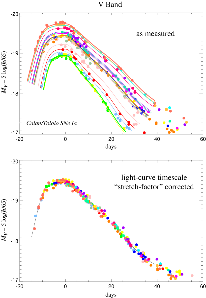
Figure 2: Type Ia supernovae exhibit a remarkable degree of homogeneity in their light curves. By fitting for one parameter, the “stretch” (Perlmutter 1997; Perlmutter et al. 1997; Goldhaber et al. 2001), the observed variation in Type Ia SNe can be reduced to $\sigma_{M}=0.15$.

3 Progenitor Models

Hillebrandt & Niemeyer (2000) provide a recent summary of the current understanding of the progenitor models for SNe Ia, and the literature reference letter of Wheeler (2003) gives a guide to the current literature. See Livio (2001) for a review of SN Ia progenitor models in the light of available observations. The prevailing progenitor model for SNe Ia is a white dwarf that accretes material from a companion star until it nears the Chandrasekhar mass ($\sim 1.4~{}M_{\odot}$) and explodes.

A key clue to the nature of SN Ia progenitors is the lack of hydrogen in their observed spectra (but see Hamuy et al. (2003); Deng et al. (2004); Wang et al. (2004); Wood-Vasey et al. (2004b)). Because of their lack of hydrogen, observed silicon, and characteristic light curves, SNe Ia are generally believed to be the result of an explosion of a degenerate object, namely a white dwarf. White dwarfs are the common endpoint in the life of stars of less than three solar masses ($M_{\odot}$). After such a star undergoes its red giant phase, it will lose its outer envelope through winds and other mass-loss events and finally leave just a carbon and oxygen core. If the core is less massive than 1.4 $M_{\odot}$, it will become a white dwarf (WD) supported by electron degeneracy pressure.

For this object to explode, it must first become unstable. A typical white dwarf will begin at $0.7M_{\odot}$ but may accumulate additional mass from a companion star until it nears the Chandrasekhar limit of $\sim 1.4~{}M_{\odot}$. As it approaches this limit, the interior conditions become unstable to fusion, and eventually a runaway fusion reaction begins at one or more points within the star and rips through the rest of the white dwarf, causing the explosion and complete destruction of the star. The additional mass required is generally significant ($\sim 0.7~{}M_{\odot}$) but could reasonably be obtained from another star as discussed in the following section. Under the assumption that the capture efficiency for two separate stars to join in a binary system after formation is relatively low, the SN Ia rate is therefore directly related to the initial binary fraction and initial mass fraction of star formation.

White Dwarf Accreting from a Companion Star (Single-Degenerate)

A common scenario for a white dwarf’s acquisition of additional mass is the accretion of material from a less-evolved binary companion in the red-giant phase. As the companion star expands, it will eventually overfill the Roche lobe of the system, causing matter to will flow from its envelope down to the surface of the white dwarf. The slowly accumulating hydrogen from this star will collect onto the surface of the white dwarf, fusing into helium and eventually carbon and oxygen (Branch et al. 1995). This model predicts that SNe Ia should result from very similar progenitor white dwarfs at the same limiting mass and thus offers an explanation for the relative homogeneity of SNe Ia. However, the accretion rate necessary to ensure the slow conversion of hydrogen to heavier elements without explosive burning and mass-loss events from the white dwarf falls in a relatively narrow range (Nomoto 1982b).

Considerations of stellar structure and evolution allow for four possible compositions for a white dwarf that nears the Chandrasekhar mass through accretion: helium; oxygen-neon-magnesium; carbon-oxygen; and carbon-oxygen with a helium shell (Branch et al. 1995; Nomoto et al. 1997; Hillebrandt & Niemeyer 2000).

Helium (He) WDs can undergo helium ignition and explode when their mass reaches 0.7 $M_{\odot}$. However, the central burning in such a process is very complete and produces just ⁵⁶Ni and unburned helium (Nomoto & Sugimoto 1977). This progenitor model fails to explain the array of intermediate-mass elements observed in the spectra of SNe Ia.

Gutierrez et al. (1996) demonstrate that an oxygen-neon-magnesium (O-Ne-Mg) star is more likely to collapse down to a neutron star than to explode. In addition, these stars are too rare to be major contributors to the observed number of SNe Ia (Branch et al. 1995).

By process of elimination, one is left with carbon-oxygen (C-O) WDs and C-O WDs with a helium shell (C-O-He) as the remaining progenitor candidates. C-O WDs form naturally in the end-of-life stage of intermediate-mass stars of up to $10~{}M_{\odot}$. For stars in this mass range, carbon fusion is the final stage of nuclear burning that balances gravitational contraction with electron degeneracy pressure. The outer envelope will be lost through the winds in the giant phase. The question then becomes how a white dwarf accretes sufficient additional mass to become unstable to a run-away fusion reaction.

The leading possibility is the so-called “single-degenerate” scenario, in which a less-evolved binary companion provides additional mass from its envelope of hydrogen or helium. If the accumulated material is hydrogen, then the accreted matter may eventually be lost through explosive hydrogen burning on the surface of the white dwarf. Depending on the rate of accumulation, which is affected by the proximity, radius, and winds of the donor star in addition to possible winds from the white dwarf, this hydrogen burning can lead to the conversion of hydrogen to helium and either the accumulation or loss of mass from the surface of the star. If the accumulated material is helium, then the white dwarf can lose mass through explosive helium burning. A well-balanced rate of accretion and fusion can lead to mass-gain through the accumulation of carbon and the eventual explosion of the entire star from an initial instability in the interior of the star.

A C-O WD can accumulate or be created with an additional layer of He. If the amount of accumulated He becomes great enough, a He flash can create a significantly off-center explosion that could tear through the star and result in an explosion of the entire white dwarf (Nomoto 1982b). However, these explosions are believed to result in either the complete conversion of the star into ⁵⁶Ni if a detonation wave is launched in the C-O or the burning of the helium only and a subsequent non-burning explosion of the C-O core (Nomoto 1982b, a; Branch et al. 1995). As with the pure helium WDs, models of C-O-He WDs do not generate the observed properties of SNe Ia.

The problems with the He, O-Ne-Mg, and C-O-He WD progenitor models outlined above leave the explosion of a pure C-O WD as the leading candidate for a SN Ia progenitor. The white dwarf is created as a C-O WD, and accreted material fuses on the surface to become part of the degenerate C-O core. When this C-O WD nears the Chandrasekhar limit, an explosion starts as either a deflagration or a detonation at some inner part of the star and proceeds outward. Detonation, or super-sonic nuclear burning, burns material completely before it has a chance to expand and so converts everything to iron-peak elements; in contrast, deflagration, or sub-sonic nuclear burning, burns while material is expanding and results in slower expansion velocities insufficient to reproduce observations of peak velocities on the order of 20,000 km/s (Hillebrandt & Niemeyer 2000). In order to explain both the high-velocities and intermediate-mass elements observed in SNe Ia, a compromise between these two models was proposed: according to this revised model, a deflagration gives the star time to expand and then transforms into a detonation at a critical transition density, $\rho_{\mathrm{DDT}}$, resulting in both intermediate-mass elements from incomplete burning of the already expanded material and high-velocities from the detonation  (Khokhlov 1991b, a; Hoeflich & Khokhlov 1996; Iwamoto et al. 1999).

White Dwarf Merger (Double-Degenerate)

The range of mass accretion rates that allow for the accumulation of mass onto a white dwarf from a main-sequence or giant companion is rather narrow. Concerns about this limited range lead to the suggestion that SNe Ia could be produced instead by the merger of two white dwarfs (Iben & Tutukov 1984; Webbink 1984). This model avoids the timing and constrained mass-loss rate problems of the single-degenerate scenario. In addition, the number of double-degenerate systems should be relatively large as both stars in a binary system will eventually evolve into white dwarfs if neither are massive enough to undergo core collapse. Eventually, the two stars will spiral inward due to energy loss through dynamic friction, their earlier respective mass-loss phases, or gravitational radiation. As the two white dwarfs near each other, they will become distorted and eventually merge. If their combined mass is near to or greater than the Chandrasekhar limit, then a runaway nuclear reaction will spread through the merged object and result in an explosion.

However, it is not immediately clear how this scenario would result in the observed homogeneity of SNe Ia. The combined mass of the white dwarfs could span a range of values that would result in a variety of explosion energy and observed light curves. This variation would be greater than the peak magnitude dispersion of $\sim 0.3$ magnitudes observed in SNe Ia (Goldhaber et al. 2001; Knop et al. 2003) but potentially could account for outliers in the SN Ia peak magnitude distribution.

Currently, the most promising model remains the C-O single-degenerate white dwarf exploding via a deflagration to detonation transition. But the other mechanisms discussed in the section may also occur and represent possible contaminants for studies requiring a homogeneous class of SNe Ia.

2 Non-Type Ia Supernovae

All other categories of supernovae (Type Ib, Ic, and II) are believed to result from the collapse of a single massive star. These supernovae can occur in multiple-star systems, but the fundamental nature of the explosion derives from the core-collapse and resulting explosive rebound of the progenitor star. These events leave behind a collapsed core, either a neutron star or a black hole, and expel the rest of their mass out into interstellar space. In a Type Ia supernova explosion, in contrast, the star is completely disrupted and no part of the original star remains. This complete destruction of the white dwarf partially explains why SNe Ia are intrinsically very bright while core-collapse supernovae vary significantly in their brightness due to different initial masses and compositions.

A core-collapse supernova occurs when the core of a massive star fuses to iron and can no longer support the star through the release of energy by fusion. The star has been steadily burning up the chain of elements, from carbon and oxygen to silicon and finally to iron. The last phase takes only seconds and leads to the collapse of the star. The core is converted into a Chandrasekhar-mass neutron star, and the infalling material compresses the core and then rebounds with a large fraction of its initial in-fall kinetic energy. This rebound develops into an explosion that blows out all of the layers above the core. In the case of more massive stars, the core rebound is sometimes not enough to let all of the infalling material escape and a black hole is created.

As the explosion proceeds through the star, layers of material are compressed and then re-expanded as the shock passes through them. This environment, far away from local thermal equilibrium, generates a wide variety of elements heavier than iron. As in SNe Ia, radioactive ⁵⁶Ni is the most common result of this shock-induced fusion and leads to the observed light curve of the supernova as the ⁵⁶Ni decays to ⁵⁶Co and then ⁵⁶Fe. However, in contrast to the relatively homogeneous SN Ia population, the variation in composition and opacities in surrounding material leads to significantly different light curve decline behaviors in different core-collapse SNe.

The initial mass of the star, the kinetic energy of the explosion, and the amount of ⁵⁶Ni produced are the three dominant factors that determine the later evolution of the core-collapse supernova light curve and spectra (Young et al. 1995). This scenario is complicated by rotation of the core, which can lead to asymmetries in the explosion, including the possible formation of jets from the poles of the rotation.

Regardless of the details of the explosion, core-collapse SNe are direct tracers of the star formation rate as they are the end stage of short-lived stars. In contrast, the progenitor systems for SNe Ia may take billions of years to evolve. This difference in progenitor lifetime means that a study of SN rates offers insight into both the star formation history of the Universe and the nature of SNe Ia progenitors.

3 Supernova Rates

Supernovae are very visible indicators of the underlying stellar population. The rates of different types of supernovae provide important clues to the evolution of the star formation rate, initial mass fraction, galaxy chemical evolution, the evolution of stellar systems, and the evolution of galaxies.

The collapse-induced explosion of massive stars is tightly linked to the initial mass fraction of the stars formed and to the overall star formation. As the most massive stars live the shortest lives, exploding within $10^{7}$–$10^{8}$ years of their formation, these types of supernovae provide a direct measure of the amount of star formation activity occurring within a given population. This population can be measured as a function of redshift, galaxy age, and galaxy composition. These supernovae are the main producers and distributors of heavy elements and thus are influential in determining the metallicities of stars in the next cycle of stellar birth.

SNe Ia, on the other hand, are believed to be the endpoint in stellar evolution for less-massive stars that form white dwarf cores in binary systems. These progenitors take at least a billion years to evolve through the main-sequence to the white-dwarf stage and yet more time to accumulate the matter to reach the critical conditions necessary for the explosion of the stars. These supernovae also contribute to the chemical evolution of the galaxy, in some ways more strongly than core-collapse supernovae, for SNe Ia release all of their material to space while the core-collapse supernovae leave behind a remnant core containing the bulk of the iron produced by the stars. However, as the core-collapse stars are more massive, they may contribute an equal amount of material to the interstellar medium on a per-supernova basis, even if the SNe Ia contribute more as a percentage of initial mass of the system. The rates of SNe Ia versus core-collapse SNe illuminate the nature of these different evolutionary pathways and are related to the star formation history of a galaxy over the past billion years (the rough time scale for a system to evolve through to a SNe Ia) to the current star formation rate. The evolution of galaxy types and morphologies is intriguingly tied into this ratio of supernova rates. As a relic of a galaxy’s history, SNe Ia also help to trace the previous evolution and state of a galaxy, even if that galaxy has since merged or been disrupted. However, as the progenitor systems of SNe Ia may wander in their host galaxy, it is possible that they are preferentially stripped from galaxies and thus more likely to be found in intra-cluster space or even outside obvious galaxies.

Studies of the absolute rate of SNe of all types are relevant to a number of questions regarding stellar evolution processes. For example, in the latter stages of life, do all massive stars end in core-collapse supernovae, or do some lose a large fraction of their mass and avoid this fate, living out their long retirement years as a white dwarf or other compact object formed without violent explosion? The initial mass fraction (IMF) of stars created may vary significantly with redshift as populations of stars live and die. Is the IMF strongly correlated with the nature of galaxy formation, or is it more dependent on more local gas density variations?

Our current limited knowledge of SN rates, particularly nearby SN rates, is insufficient to provide good constraints on galactic and stellar populations and evolution. Even the basic rate of SNe Ia is only constrained to $30\%$ at $z\sim 0.01$ (Cappellaro et al. 1999a) and $15\%$ at $z\sim 0.5$ (Pain et al. 2002). The rate for SNe Ia at $z\sim 0.1$ is only known to within a factor of 2 (Cappellaro et al. 1999a). A determination of the local SN Ia rate to the same precision as the high-redshift SN Ia rate would allow for a study of star formation rates and offer further clues to the nature of SN Ia progenitors.

4 Cosmology with Redshifts and Luminosity Distance

The homogeneity of SN Ia light curves can be exploited to make cosmological measurements by employing the SN Ia redshifts and standardized peak magnitudes to determine the relationship between the scale factor of and luminosity distance in our Universe. See Weller & Albrecht (2002) for a useful summary of deriving cosmological results from SNe Ia. Briefly, the redshift, $z$, is a relative measurement of the cosmological scale factor, $a$, at the epoch of the supernova,

$$\frac{a_{0}}{a}=1+z,$$ (1)

where $a_{0}$ is the present-day scale factor. The observed, or apparent, peak magnitude, $m$, of a SN Ia is used to determine its luminosity distance, $d_{L}$, defined by

$$f_{\mathrm{o}bserved}=\frac{L_{\mathrm{s}ource}}{4\pi d_{L}^{2}},$$ (2)

where we consider the bolometric flux $f$ and bolometric luminosity $L$. Recall that magnitudes are defined as the logarithm of the flux,

$$m=-2.5\log_{10}{f}=-2.5\log_{10}{\frac{L_{\mathrm{s}ource}}{4\pi d_{L}^{2}}}=-2.5\log_{10}{L_{\mathrm{s}ource}}-5\log_{10}{d_{L}}-2.5\log_{10}{4\pi},$$ (3)

modulo constants that defines the distance units and magnitude zeropoint. By convention, absolute magnitudes are defined at a luminosity distance of 10 parsecs (pc). The difference between the absolute magnitude, $M$, and apparent magnitude, $m$, of an object is defined as the distance modulus, $\mu=m-M$, and is related to the luminosity distance as follows:

$$m-M = (-2.5\log_{10}{L_{\mathrm{s}ource}}-5\log_{10}\frac{d_{L}}{[{\mathrm{p}c}]})-(-2.5\log_{10}{L_{\mathrm{s}ource}}-5)$$ (4)

$$\mu = +5-5\log_{10}{d_{L}}{[{\mathrm{p}c}]}$$ (5)

$$\mu = -25-5\log_{10}{d_{L}}{[{\mathrm{M}pc}]}$$ (6)

$$d_{L} = 10^{-(\mu+25)/5}~{}[\mathrm{Mpc}].$$ (7)

Any class of bright astrophysical objects that occur at redshifts out to $z\sim 1$ with a constant $M$ can be used for cosmological measurements by using the redshift and Eq. 7 of these objects to determine the geometry and expansion history of the Universe.

Figure 3: The SN Ia luminosity distance-scale factor relation used to measure the expansion history of the Universe. On the left, the luminosity distance modulus, $\mu=m-M$, versus inverse scale factor. On the right, the SN Ia effective magnitude in the B-band optical filter, $m_{B}$, versus redshift, shown on a log scale for the redshift. This $m_{B}$ vs. $\log{z}$ format is the more commonly seen presentation. Note that the absolute normalization of the distance modulus is dependent on the assumed values for $H_{0}$ and $M$ but is unimportant in the cosmological measurement of $\Omega_{M}$ and $\Omega_{\Lambda}$. The low-redshift, ($a_{0}/a\sim 1$), region is clearly a critical anchor point for comparison with higher redshift measurements. (Data from Riess et al. (2004))

The homogeneity of SN Ia light curves (Branch & Tammann 1992; Branch & Miller 1993) allows for relative luminosity distances to be calculated quite accurately and led to the use of SNe Ia as standardizable candles in studies of the geometry and expansion history of the Universe (Perlmutter et al. 1997). As an astronomical measurement of $d_{L}$ involves a comparison of $m$ and $M$ (Eq. 7), the key benefit of using SNe Ia is that they have very similar absolute magnitudes, $M$, at peak. Thus, one can construct a plot of $d_{L}$ versus $a_{0}/a$ (see Fig. 3) to reveal the expansion history of the Universe. The $H_{0}$ dependence of $d_{L}$ and $M$ can be separated out into

$$\mathcal{D}_{L} = H_{0}d_{L}$$ (8)

$$\mathcal{M} = M-5\log_{10}H_{0}+25$$ (9)

and thus one can rewrite Eq. 5 with no $H_{0}$ dependence as

$$m-\mathcal{M}=5\log_{10}\mathcal{D}_{L}.$$ (10)

To fit for the cosmology underlying $\mathcal{D}_{L}$, one then performs a joint fit from low to high redshift and marginalizes over $\mathcal{M}$. Alternatively, if one had a well-constrained value for $\mathcal{M}$ from a sample of a few hundred nearby SNe Ia in the smooth Hubble flow, one could use this value in Eq. 10 when fitting higher-redshift supernovae. Ultimately, the cosmological results are dependent on having a source with a relatively constant $M$ over a large range of redshifts and are not specifically dependent on either $M$ or $H_{0}$.

As Eq. 7 shows, it is only the difference between $m$ and $M$ that enters in the calculation of $d_{L}$. The low observed scatter in $M$ allows for $m-M$ to be a useful indicator of luminosity distance. The Hubble constant, $H_{0}$, represents a constant offset in the distance scale, but it is not important in the measurement of the change of $d_{L}$ with $a$.

After it was demonstrated that SNe Ia could be discovered in a reliable manner that allowed for planned and scheduled follow-up (Perlmutter et al. 1997), two independent teams measured luminosity distances and redshifts to high-redshift SNe Ia and concluded that there was a significant non-matter component of the total energy density of the Universe that has been causing the Universe to increase its rate of expansion over the past seven billion years (Perlmutter et al. 1998; Garnavich et al. 1998; Riess et al. 1998a; Perlmutter et al. 1999). This unknown component became known as “dark energy,” and its nature and source remains the biggest mystery in cosmology and particle physics today. For further progress to be made in this important field, better understanding of the residual variation of SN Ia light curves is necessary.

As cosmology has progressed and galaxy clustering studies (Turner 2001; Allen et al. 2002; Bahcall et al. 2003; Tegmark et al. 2003) and cosmic microwave background measurements (Jaffe et al. 2001; Bennett et al. 2003; Spergel et al. 2003) agree with the supernova results, we are entering the age of precision cosmology. Further understanding of the history and evolution of the Universe will come from the next generation of supernova cosmology experiments.

The next great project is measuring the equation of state of the Universe (Weller & Albrecht 2002). While it may appear most natural to consider the luminosity-distance vs. redshift measurements in terms of the scale factor $a$, many models attempting to explain the nature of dark energy are framed in terms of the equation of state of the dark energy (Linder 2003). Specifically, these models predict values for the ratio, $w$, between the pressure, $p$, and density, $\rho$, of the dark energy:

$$w=\frac{p}{\rho}.$$ (11)

Most simply, if the current acceleration of the Universe is caused by a cosmological constant, then $w=-1$ is constant with time. For models where $w$ evolves with the scale factor, $a$, $w$ can be parameterized as

$$w=w_{0}+w_{a}(1-a)$$ (12)

(see Linder (2003)). While Eq. 12 implies a linear variation with $a$, in general $w$ could be any arbitrary function of $a$ (see Linder & Jenkins (2003)).

Models predicting a constant $w=w_{0}$, including those invoking a cosmological constant, are the easiest to test. Two projects are presently underway to measure $w_{0}$ to $\sim 10\%$ using SNe Ia from $0.3\mathrel{\hbox{\hbox to0.0pt{\hbox{\lower 4.0pt\hbox{$\sim$}}\hss}\hbox{$<$}}}z\mathrel{\hbox{\hbox to0.0pt{\hbox{\lower 4.0pt\hbox{$\sim$}}\hss}\hbox{$<$}}}0.8$. The SuperNova Legacy Survey (SNLS) (Pritchet & Collaboration 2004) is a part of the Canada-France-Hawaii Telescope Survey (The CFHTLS Supernova Program 2004) and will discover and study 2000 SNe Ia between 2003 and 2008. The ESSENCE project (The ESSENCE Team 2003) is undertaking a similar study using the CTIO 4.0-m telescope to compile a data set of $\sim 500$ SNe Ia by 2006. Both projects use 8-m class telescopes for spectroscopic confirmation and study. The current scatter of $0.10$–$0.15$ magnitudes in the luminosity-distance indicator currently used for SNe Ia and the lack of well-observed nearby SNe Ia have become the central limitations in using SNe Ia to measure $w$.

The need for improved phenomenological and systematic calibration of SNe Ia and the current lack of a high-quality sample of SNe Ia at low redshift demand a comprehensive study of nearby SNe Ia. Meeting the goals of the SNLS and ESSENCE projects will require a large sample of nearby supernovae on the same order as the many hundreds of distant SNe Ia to be found by each project to enable a comparison of low- and high-redshift SNe Ia.

While a sample of nearby SNe Ia will provide improved statistical constraints on the luminosity-distance-redshift Hubble diagram, there is a more pressing need for an improved understanding of and controls on systematic errors in using SNe Ia to make cosmological measurements. It is critical to constrain possible systematic effects so that any evolution with redshift can be quantified. An improved understanding of the astrophysical processes underlying SNe Ia and their progenitors will be invaluable in elucidating the residual variation seen in SN Ia light curves.

5 Needed Improvements for SN Ia Cosmology

SNe Ia exhibit a surprising degree of homogeneity in their absolute brightness. They are observed to vary in peak B-band brightness by only $\sim 30\%$ (Goldhaber et al. 2001). This variation can be reduced by the use of a time-scale parameter that characterizes the observed relationship between light-curve width and brightness for SNe Ia (Pskovskii 1970, 1977; Phillips 1993; Hamuy et al. 1995; Riess et al. 1995, 1996; Perlmutter 1997; Goldhaber et al. 2001) (see Fig. 2). Phillips (1993) found that SNe Ia exhibited a dispersion in their intrinsic brightness that was correlated with their magnitude decline rate after maximum light, $\delta m_{15}$. Other parameterizations of this correlation result in a residual scatter in SN Ia maximum B-band luminosity of $0.15$ magnitudes (Riess et al. 1996; Hamuy et al. 1996; Perlmutter et al. 1997; Phillips et al. 1999). This $\sim 15$% level of standardization was sufficient for the original cosmological measurements that provided clear evidence for an accelerating Universe.

The MLCS (Riess et al. 1995, 1996), $\Delta m_{15}$ (Phillips 1993; Hamuy et al. 1995, 1996) and stretch (Perlmutter et al. 1997, 1999) methods currently used are all equivalent to the variation of a single parameter. See Figure 2 for an example of how the stretch parameter unifies light curves from a group of SNe Ia. The large sample of high-resolution SN Ia spectra provided by the SNfactory will hopefully provide additional parameters that will improve the current standardization of luminosity distances from SNe Ia. A detailed set of spectra from a large, well-studied population will bring improved understanding of both the known first-order and surmised higher-order variations in SN Ia light curves.

As efforts continue to measure the expansion history of the Universe to higher precision and more SNe Ia are added to the Hubble diagrams used to fit for the cosmological matter density and dark energy density, the residual dispersion and unknown systematics of SN Ia magnitudes are becoming a significant source of uncertainty.

The dominant source of uncertainty in using SNe Ia for cosmological measurements is in the luminosity distance of the SNe Ia. This uncertainty arises both from measurement error of the SN flux and, more importantly, from variations in the absolute brightness of SNe Ia. The redshift to a given SN host galaxy can be measured very precisely from galactic emission lines and is only a significant source of uncertainty at low redshift where peculiar velocities dominate over the Hubble flow expansion.

It is unknown whether the residual dispersion in SN Ia light curves after fitting for the time-scale parameter, is simply a random distribution with no correlation with possible observables or whether there is a second parameter that could reduce this scatter even further. If the dispersion is random, then very large numbers of supernovae will be required to reduce the overall uncertainties. Even then, unknown and uncontrolled systematic uncertainties could limit the accuracy of any such measurement. While correlations have been observed between selected SN Ia spectral features and the $\Delta m_{15}$ time-scale parameter (Nugent et al. 1995; Mazzali et al. 1998; Riess et al. 1998b; Hatano et al. 2000), a detailed analysis of a large sample of SN Ia spectra will be necessary to search for improved spectroscopic indicators that allow for a deeper understanding and better standardization of luminosity distances measured with SNe Ia. If correlations are found with such secondary observables, then future high-redshift supernova studies will greatly benefit from the improved calibration possible from a better understanding of SN Ia properties. The calibration of these vital standardizable candles needs to be significantly improved to allow the next generation of large-scale missions, such as the SuperNova Acceleration Probe (SNAP) (Aldering et al. 2004) and the Joint Dark Energy Mission (JDEM), to explore the dark energy and expansion history of the Universe.

Part 1 The Nearby Supernova Factory

Chapter 1 The Nearby Supernova Factory

Please see Appendix 8 for a conference proceedings article (Wood-Vasey et al. 2004a) that provides a brief summary of the Nearby Supernova Factory mission and the results from the prototype supernova search.

1 Concept

In order to fill the vital need for a well-observed sample of nearby SNe Ia, the Nearby Supernova Factory (SNfactory) project (Aldering et al. 2002a; Pécontal et al. 2003; Wood-Vasey et al. 2004a) has been devised to discover and study in detail $300$ SNe Ia to better understand and calibrate these important cosmological tools. The SNfactory aims to provide a definitive data set for nearby SNe Ia by observing a large and diverse sample of SNe Ia to provide a comprehensive sample of the parameter space of observed SN Ia variation for comparison with higher-redshift SNe Ia.

Further progress in supernova cosmology requires an order-of-magnitude increase in the number of well-studied SNe Ia in the nearby smooth Hubble flow ($0.03<z<0.08$) to provide a better understanding of luminosity distance indicators for SNe Ia and to anchor the low-redshift end of the SN Ia Hubble diagram (see Fig. 3). A two-fold reduction in the scatter of the SN Ia luminosity-distance indicator would yield a commensurate improvement in the constrains on $w_{0}$ (see Sec. 4). Even without this better calibration of SNe Ia, the statistical weight of the 300 SNfactory SNe Ia alone will provide a factor of two improvement in both the SNLS (Pritchet & Collaboration 2004) and ESSENCE (Garnavich et al. 2002) measurements of $w_{0}$ and the SNAP (Aldering et al. 2004) measurement of $w_{a}$. The improved calibration of SNe Ia that the SNfactory will allow is also a critical contribution needed to make full use of the large number of SNe Ia that will be found and studied with current and upcoming intermediate- and high-redshift projects such as ESSENCE, SNLS, and SNAP.

The data set acquired by the SNfactory will be a rich source of information about the SNe Ia themselves. From the nature of their progenitors to their rate of their occurrence, many mysteries remain regarding these useful cosmological standards. Detailed, early-time spectra of SNe Ia will constrain SN Ia progenitor models and provide clues to the observed variation in SN Ia light curves. A proper understanding of the efficiency and selection biases in a SN search is critical to a proper determination of SN rates, for which the large, automated search of the SNfactory will be an excellent source. The SNfactory sample of 300 $z\mathrel{\hbox{\hbox to0.0pt{\hbox{\lower 4.0pt\hbox{$\sim$}}\hss}\hbox{$<$}}}0.1$ SNe Ia will allow for a determination of the nearby SN Ia rate to $\sim 6$% to provide useful constraints on galactic and stellar evolution models.

The first crucial part of the SNfactory project is to discover large numbers of supernovae in the nearby Hubble flow ($0.03<z<0.08$) in a reliable, continuous fashion. Discovering hundreds of SNe Ia in this redshift range requires searching of hundreds of square degrees of sky every night. To cover this much area, the SNfactory uses an automated image processing and subtraction pipeline, developed as a major focus of the dissertation work presented herein, to scan images from nightly wide-field asteroid searches. This pipeline has discovered $83$ SNe in its prototype phase of operation. See Chapters 2 & 3 for a description of this successful supernova search project.

The second component of the SNfactory project is spectrophotometric follow-up of the SNe, using a custom-built instrument dubbed the SuperNova Integral Field Spectrograph (SNIFS). This specialized instrument takes spectrophotometric observations of an object and its surroundings by using an array of $225$ lenselets fully covering a 6-arcsecond by 6-arcsecond region. This array allows for simultaneous observations of SNe Ia and their host environment in an automated fashion. In parallel with the spectrograph, SNIFS has a multi-color photometric channel that allows for precise flux-calibration of the observed spectra by monitoring the atmospheric extinction during the spectral exposure. See Lantz (2003) for a description of the SNIFS instrument.

SNIFS is mounted on the University of Hawaii 2.2-m telescope and is integrated into the SNfactory search pipeline to automatically confirm and follow supernovae. Spectrophotometric observations will be taken every $3$–$5$ days from well before maximum light through several months after explosion. SNIFS is in the final stages of commissioning and the SNfactory will begin full, integrated operations in late-2004.

2 Goals of the Nearby Supernova Factory

1 New SN Ia Luminosity Distance Indicator Parameterization

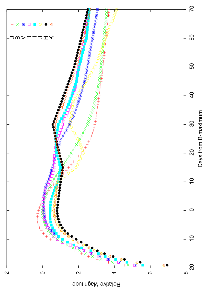
Figure 1: Schematic light curves of a SN Ia in different standard astronomical filters. Template courtesy of Peter Nugent. See Goldhaber et al. (2001) for a more complete discussion of SN Ia light curves and templates.

Current SNe Ia calibration techniques use one parameter to describe all of the observed variation in SNe Ia light curves (see Sec. 5). The major physical explanation for the observed variation in SNe Ia light curves is differing amounts of ⁵⁶Ni created in the explosion. As the light curves of SNe Ia are determined by the decay of ⁵⁶Ni, variations in the amount of ⁵⁶Ni produced could lead to the observed variations in peak brightness that follow the width-luminosity relation illustrated in Fig. 2. Models producing different amounts of ⁵⁶Ni exhibit a width-luminosity relation similar to that observed, but they do not plausibly account for the peculiar SNe Ia like SN 1991T (over-luminous, $1.0$ $M_{\odot}$ ⁵⁶Ni (Spyromilio et al. 1992)) or SN 1991bg (under-luminous, $0.1$ $M_{\odot}$ ⁵⁶Ni (Filippenko et al. 1992)) (Mazzali et al. 2001) .

The chemical composition of the progenitor system of a SN Ia is another physical mechanism that could lead to differences in observed peak brightness. The metallicity of the explosion, if not the progenitor itself, can be studied by an examination of spectral features characteristic of different elements formed in the explosion. The quantity of most obvious interest is the ratio of carbon and oxygen in the progenitor star. This ratio directly affects the abundances of elements created in the nuclear burning of the explosion. Since the decay of ⁵⁶Ni is the primary source for the observed optical luminosity of the SN, variations in the amount produced of this radioactive element can have a significant effect on the luminosity of the SN Ia.

Indirectly, the light curve can also be affected by hydrodynamic differences in the exact nature of the detonation/deflagration process that produced the SN Ia. A variety of models and simulations exist that address these issues, but they await detailed observations to differentiate between them.

The SNfactory data set will allow for calibration and comparison of supernova light curve shapes in any optical color. With photometric spectroscopy, the SNfactory will be able to synthesize a light curve at any redshift for any given filter matching a rest-frame wavelength range from $3500$–$10000$ Å, producing a set of high-quality SNe Ia template light curves for use in comparison with higher-redshift SNe Ia. Reconstructing synthesized light curves from the SNfactory flux-calibrated spectra at rest-frame wavelengths in the standard astronomical filters (e.g. $UBVRI$ or $ugriz$) will allow for immediate recalibration of existing intermediate- and high-redshift SN Ia data sets through a new understanding of the family of SN Ia light curves. This improved set of template light curves will allow for a comprehensive analysis of width-luminosity and color-color relationships (Wang et al. 2003b) in different filters.

2 Providing a Definitive Set of SN Ia Spectra

K-corrections

While the SNfactory data set will allow for in-depth analyses to address questions regarding the physical nature of SNe Ia, an immediate benefit of the SNfactory data will be an improved phenomenological understanding of SNe Ia. In particular, this comprehensive set of SN Ia spectra will cover the diversity of the SN Ia family and will be invaluable in improving K-corrections for observed magnitudes of SNe Ia (Kim et al. 1996; Nugent et al. 2002).

Observations of SNe Ia are generally conducted in several different filters for comparison of their light curves and absolute magnitudes. When comparing SNe at different redshifts, it is important to properly correct the magnitudes in each filter by the amount of the spectrum shifted into and out of the filter bandpass as the redshift shifts the spectrum to longer wavelengths. These adjustments are known as K-corrections. For an object with a complicated spectrum such as a SN Ia, it is important to track the spectral features as they move through the different filters. Correcting appropriately for this redshift effect requires a detailed knowledge of the spectrum of the supernova at every epoch. Ideally, for every distant supernova, one would like a spectrum of a well-studied nearby supernova that is a good match to the distant one. This like-to-like matching necessitates having a spectrum of a nearby supernova at every possible epoch for every different type of supernova.

The SNfactory data set will provide a valuable resource for both quantifying SN Ia diversity and establishing the new standard reference for SNe Ia spectra. Most critically, the SNfactory spectra will provide for direct matches with photometrically observed high-redshift SNe Ia. The K-correction can be done with the high-quality spectrum that is the best match out of the 300 SNfactory SNe Ia. This comprehensive spectral database will bring deterministic clarity to the current art of K-corrections (Leibundgut 1990; Hamuy et al. 1993; Kim et al. 1996; Nugent et al. 2002).

Dust extinction correction

The spectrum of a supernova is affected by the presence of dust along the line of sight to the supernova. Dust between an observer and an object will both dim and redden the observed flux from the object. This dimming can be parameterized as a function of wavelength (Cardelli et al. 1989; O’Donnell 1994). By taking advantage of this relationship, the brightness of SNe Ia can be corrected for extinction by taking the color differences between the observed supernova spectrum and a reference supernova spectrum from an extinction-free region. The latter generally come from elliptical galaxies, as they are relatively free of dust in comparison to spiral galaxies. The number of supernova available for this color-based extinction correction is currently quite small and more are needed to minimize the uncertainty in this correction.

The need for well-established intrinsic colors extends beyond just correction for dust extinction. Dust is generally smooth in its absorption variation over wavelength, but obtaining a pure spectrum, unadulterated by host-galaxy dust, is still necessary to reduce our reliance on the assumption that the effects of dust are understood. Dust from the inter-galactic medium and our own galaxy is, of course, unavoidable, but the former can be observed separately from the SN while the latter has been well-studied (Schlegel et al. 1998).

3 Study of host galaxies

Studies of the host galaxies of SNe Ia will help answer questions about the effects of environment on the formation and explosion of SNe Ia. The specialized integral field unit spectrograph built by the SNfactory will allow for simultaneous observations of both a supernova and its host galaxy. Sufficiently large or nearby hosts will be covered by several separate lenses. Such spatial coverage will allow for a systematic study of host galaxy properties and morphology, which is the closest we will ever be able to come to examining the host environment of a Type Ia supernova. The actual birthplace of the SN Ia progenitor is perhaps impossible to truly determine as the likely progenitors for SNe Ia are white dwarfs (see Sec. 3), which can be billions of years old and have thus had the opportunity to leave their stellar birthplace and wander about their host galaxy.

3 Operational Strategy

A coordinated observational program is vital to accomplishing the ambitious scientific goals of the SNfactory. The expertise gained from many successful supernova programs, in particular a large pilot program organized by the Supernova Cosmology Project in the spring 1999, has gone into the design of the SNfactory integrated search and follow-up pipeline and it is carefully constructed to yield a homogeneous sample of SNe Ia suitable for answering the key questions discussed above.

1 Detection

The SNfactory will focus on SNe Ia in the smooth linear Hubble flow ($0.03<z<0.08$). SNe Ia in this redshift range are sufficiently close to allow for high signal-to-noise observations but are sufficiently distant so that the redshift is a good indicator of distance (see Fig. 2). In addition, these SNe Ia will be close enough so that the non-linear expansion history of the Universe will not have a large effect on the luminosity-distance for these supernovae.

Figure 2: The SNfactory is operating in the “sweet spot” between peculiar velocity noise and cosmological uncertainty. The SNfactory histogram is the redshift distribution of SNe shown in Fig. 2 scaled up to 100 SNe/year. The known-galaxy search curve has also been scaled to 100 SNe/year. The peculiar velocity of local galaxies, taken here to be 300 km/s (Landy 2002), dominates low-redshift part of the “Velocity+Cosmology Error” curve. The cosmological uncertainty shown here is the difference in distance modulus in an $\Omega_{M}=0.3$, $\Omega_{\Lambda}=0.7$ Universe and an $\Omega_{M}=0.3$, $\Omega_{\Lambda}=0$ Universe.

The supernovae will be found using data from automated nightly wide-field asteroid searches and will be studied from several weeks before through several months after maximum brightness of the supernovae. It is necessary to search a large area of the sky every night, $\sim 500~{}\hbox{\hbox to0.0pt{$\sqcap$\hss}$\sqcup$}\hbox{${}^{\circ}$}$, to find enough SNe Ia soon after their explosion to study 100 SNe Ia per year. The volume of space out to a redshift of $z=0.08$ is limited; on a given search night only $\sim 0.01$ SNe Ia are expected to be detected before maximum light in any particular square degree out to a limiting depth of $20.5$ magnitudes.

The SNfactory currently discovers supernovae using images from a collaboration with the Near-Earth Asteroid Tracking (NEAT) group at the Jet Propulsion Laboratory. In their quest for asteroids, the NEAT scans the skies every night and looks for objects that move over the time scale of an hour. They take three images of a given field in the sky, spaced fifteen–thirty minutes apart, and search for objects which move by more than a couple of arcseconds over this period. They do this for hundreds of fields every night, covering $500$–$1000$$\sqcap$$\sqcup$^∘. This strategy enables them to find thousands of new asteroids in the main asteroid belt of our solar system and near-Earth asteroids in particular. The SNfactory uses these data and compares the new images with reference images of the same field from previous years of NEAT data by subtracting the reference image from the new image and looking for the objects which remain.

The SNfactory search pipeline has been quite productive in a several-year collaboration with the NEAT group. In addition, a new arrangement with the Palomar Consortium became effective in 2004 and is expected to be equally productive. Chapter 2 explains how the SNfactory uses both the NEAT and Palomar Consortium data to search for supernovae.

2 Study

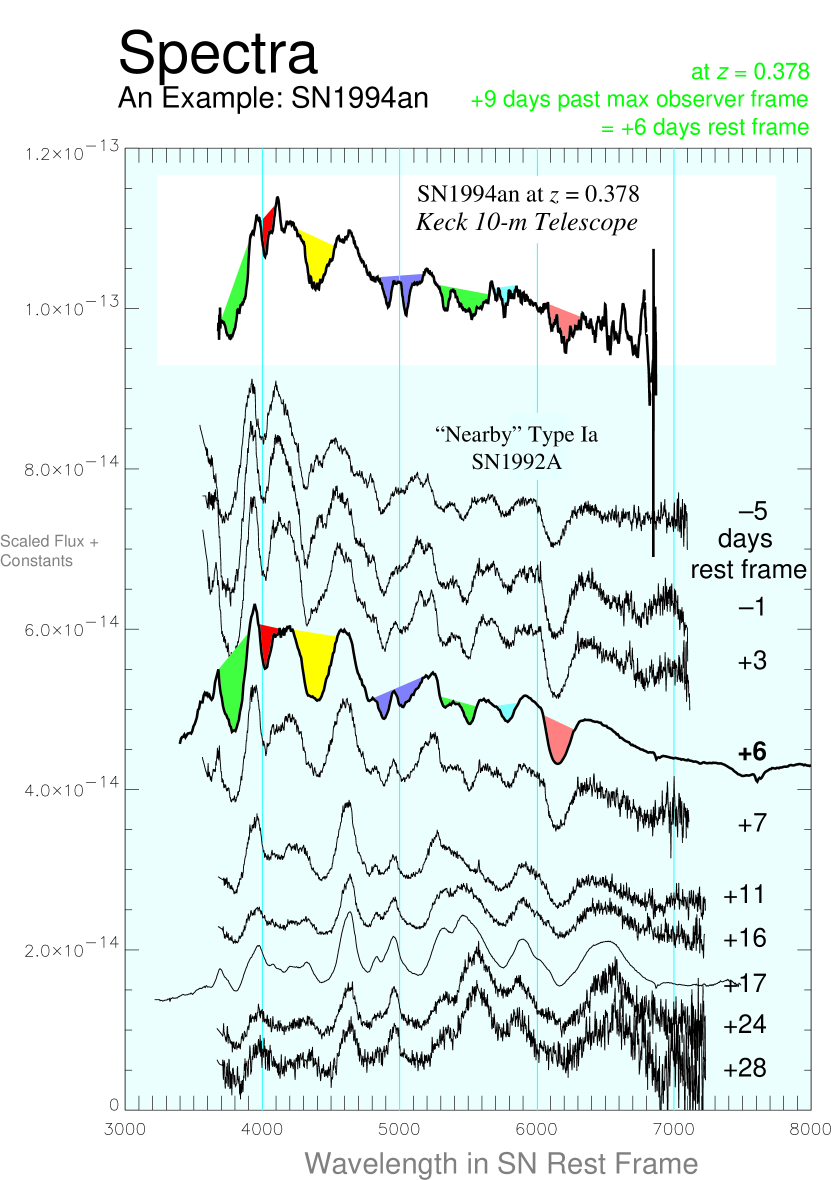
Figure 3: Type Ia supernovae exhibit remarkable uniformity in their spectral evolution but show differences in specific spectral features (illustrated here by colored regions) that may provide clues to better calibrate their luminosity distances.

A systematic study of hundreds of SNe Ia calls for an automated, guaranteed-time follow-up strategy. The goals of the SNfactory project require $12$–$15$ spectroscopic and photometric observations of each SN Ia. Fig. 3 gives an example of this type of coverage for SN 1992A, although the SNfactory coverage will extend to earlier and later epochs in the evolution of the SNe Ia. The spectroscopic precision required for spectrophotometric-quality observations necessitates an instrument specially designed for the purpose. To enable the comparison and study of features across the entire observed wavelength regime, the spectroscopic observations must be flux-calibrated to within one percent. This precision allows for photometry to be reconstructed for any optical filter. Practically speaking, the precision alignment required to operate a traditional slit-spectrograph in an automated mode is quite a challenge. Few telescopes have the pointing precision to line-up a target object to within the $0.5$^′′ necessary for traditional slit spectroscopy. An integral field unit (IFU) spectrograph obviates both static and wavelength-dependent slit loss by collecting all of the light in a region through an array of imaging elements covering 99% of the total area.

SNIFS is a dedicated instrument built specifically for the SNfactory project. With two spectroscopic channels ($3000$–$5500$ Å and $5500$–$10000$ Å) and an integrated photometric monitoring and guiding camera, SNIFS will provide flux-calibrated spectroscopy through automated observation. It features a $6\hbox{${}^{\prime\prime}$}\times 6\hbox{${}^{\prime\prime}$}$ field-of-view covered by an array of $15\times 15$ lenselets (with $99\%$ coverage). This IFU allows for both simultaneous observation of a supernova and its host galaxy and for a reduction in the pointing precision required to $\pm 1\hbox{${}^{\prime\prime}$}$. The SNIFS photometric channel features a custom-built multi-filter that simultaneously monitor five bandpasses to measure sky absorption and seeing in parallel with the spectroscopic observations.

As of June, 2004, the SNIFS instrument has just been successfully commissioned at the University of Hawaii 2.2-m telescope. The automated operation and spectrophotometric observations provided by SNIFS on the UH 2.2-m. will allow the SNfactory to obtain observations of the hundred supernovae a year required by this ambitious project.

4 Summary and Plan for Subsequent Chapters

The current intrinsic dispersion in SN Ia peak magnitudes and associated systematic uncertainties will soon become the limiting factor in our determination of the geometry and expansion history of the Universe using SNe Ia. It is necessary to improve our understanding and knowledge of SNe Ia before we can proceed with the next generation of distant supernova searches. The integrated detection pipeline and dedicated follow-up resources of the SNfactory will allow for a detailed study of 300 SNe Ia that will provide a critical foundation for the future of supernova and supernova cosmology science.

The following three chapters discuss details of the search aspects of the SNfactory, which was the primary focus of this dissertation work. Chapter 2 covers the operation of the SNfactory search pipeline. Chapter 3 details the subtraction software used to detect supernovae. Chapter 4 describes the supernovae found in the prototype search of the SNfactory. For further discussion of the follow-up aspects of the SNfactory project, see Aldering et al. (2002a) and Lantz (2003).

Chapter 2 Search Pipeline Design and Implementation

1 To catch a supernova

The SNfactory search pipeline discovers supernovae using images obtained in collaboration with the Palomar Consortium (Yale/JPL/Caltech) and the Near-Earth Asteroid Tracking (NEAT) group at the Jet Propulsion Laboratory. The NEAT group uses the Palomar 1.2-m Samuel Oschin and Haleakala 1.2-m MSSS telescopes in its search for near-Earth objects while the Palomar Consortium encompasses a variety of projects using the Samuel Oschin 1.2-m, including searches for quasars, supernovae, and trans-Neptunian objects. The NEAT program scans portions of the sky every night and returns to the same fields every seven to fourteen days. The Palomar Consortium uses the Oschin 1.2-m telescope in drift-scan mode, typically covering a more limited area of sky than the NEAT program and observing each field only once per night, repeating the fields a few days later for the purposes of SNe searching. The SNfactory uses the repeated coverage from both types of observations to search for new point sources. The search pipeline compares the old (“reference”) and new (“search”) images of the same field by subtracting the reference image from the search image and looking for the objects that remain. These are the candidate supernovae. Fig. 1 shows an example of this process for the discovery of SN 2001dd.

This ostensibly straightforward process of searching via image subtraction turns out to be more complex than it may at first appear. The presence of detector artifacts and variations in the image quality of reference images and search images are some of the most significant challenges. The search pipeline uses a sophisticated suite of image tools, but up to the present time the final step in the vetting process still requires human input to separate the good supernovae candidates from the bad. On the order of one percent of the search images taken are found by the automated processing and subtraction software to have a potentially interesting object. Roughly one percent of those objects turn out to be supernovae.

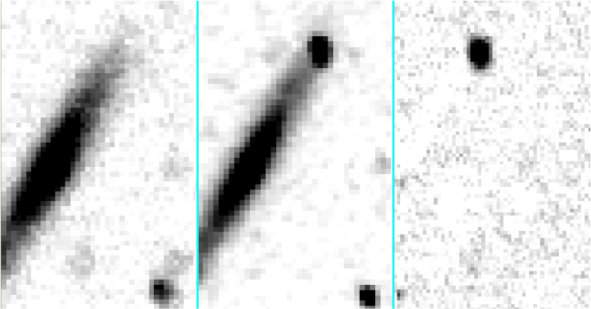
Figure 1: (left) A reference image taken on 16 January 2001 (UT) showed the galaxy. (center) A search image taken on 30 June 2001 (UT) showed the same galaxy with a brighter region. (right) Subtracting the reference image from the search image yielded a new object, which was confirmed to be a Type Ia supernova. Note that the galaxy and the star in the lower-right both disappear in the subtracted image. The area shown here represents a small fraction a typical search image.

From the fall of 2002 through the spring of 2003, a systematic search for supernovae was carried out with the Palomar 1.2-m Samuel Oschin telescope. In 2001, the NEAT group outfitted this telescope with an automated control system and added a 3-chip 3$\sqcap$$\sqcup$^∘ field-of-view (FOV) CCD camera (NEAT12GEN2) at the spherical focal plane at the primary focus of this Schmidt reflector. In April of 2003, this camera was replaced by the QUEST group at Yale with a 112-chip 9$\sqcap$$\sqcup$^∘ FOV detector (QUESTII) capable of both drift-scan and point-and-track observations. QUESTII became fully operational in August of 2003. The SNfactory also processes data from the Haleakala MSSS 1.2-m. telescope with the NEAT4GEN2 detector. These images are not currently included in the SNfactory search because of their poor quality and under-sampled resolution.

2 Processing Steps toward Supernova Candidates

The SNfactory pipeline has the ability to automatically process and search images from all of the aforementioned telescopes through a well-defined processing framework. The basic image cleaning routines were adapted from the Supernova Cosmology Project (SCP) Deeplib C++ framework. The processing of the NEAT data is described below. The same steps apply to images from the NEAT4GEN2, NEAT4GEN12, and QUESTII detectors taken using the telescopes’ point-and-track mode. A special section on the differences involved in the processing the drift-scan data from the Palomar Consortium follows. The specific details of the implementation presented here apply to the SNfactory plans and setup as of the spring of 2004.

The basic search sequence is as follows:

2. Obtain reference images.

3. Reduce reference data.

4. Obtain search images.

5. Reduce search images.

6. Perform subtractions.

7. Perform automated scanning.

8. Perform human scanning.

9. Perform cross-checks.

10. Obtain confirmation image.

11. Obtain confirmation spectrum.

12. Report discovery.

The sections that follow discuss the SNfactory’s implementation of these steps. In the sections below, the discussion of the processing steps will diverge a little from the order in which they are presented above. The discussions of the observation and image reduction steps will be combined because these processes are the same for both reference and search images.

3 Sky Coverage

Using the Oschin and MSSS telescopes, the NEAT group takes many images of the night sky over a range of right ascension (RA) and declination (Dec). All sky fields are covered in at least three exposures spread over approximately an hour. This temporal spacing allows the NEAT group to search for asteroids at the same time that it enables the SNfactory search pipeline to eliminate those same asteroids and to minimize contamination due to cosmic rays. Ideally, the fields obtained cover some simple rectangle on the sky to facilitate later searching images and to provide a complete set of references for future searches in later years. In practice, the coverage pattern is more complicated. A significant challenge for the SNfactory project was transferring all of these imaging data (up to 60 GB/night) to the computing resources necessary to process the images.

4 Data Transfer from Palomar to LBL

The image data are obtained from the telescope and stored at Lawrence Berkeley Laboratory (LBL) on the National Energy Research Supercomputing Center (NERSC) High Performance Storage System (HPSS). From there, the images are transferred to the NERSC Parallel Distributed Systems Facility (PDSF) (see Fig. 2). This cluster comprises approximately 200 Dual 1-GHz Pentium IV PCs with 2 Gigabytes (GB) of memory and 50 GB of scratch disk space apiece. Processes are scheduled on the cluster using the Sun Grid Engine software package.

As each image is read-out from the telescope, it is saved in a compressed format to local disk space. There are currently several hundred gigabytes of storage at the observatory for this purpose. This storage capacity allows for the 20–50 GB/night of data in compressed form to be stored with space to buffer several nights of data in cases of transmission failure.

A high-speed, 45 Megabit-per-second (Mbps) radio internet link has been established between the Palomar Observatory and the San Diego Supercomputer Center (SDSC) as part of the High Performance Wireless Research and Education Network (HPWREN) (Braun 2003). This link is used to transfer the images from Palomar to HPSS in near real time. The 45 Mbps bandwidth comfortably exceeds the data rate from the telescope. The bandwidth from SDSC to LBL and NERSC is excellent and several orders of magnitude greater than necessary to meet the transfer requirements.

The observing plan for the NEAT12GEN2 detector used from 2001–2003 put the telescope through three pointings every four minutes. There were 3 CCD detectors on the instrument so each pointing resulted in 3 images. These images were spaced about 1 degree apart in declination. Each image was $32$ Megabytes (MB) in its raw form but was compressed to $\sim 16$ MB for transfer. This produced $144$ MB of data to be transfered every four minutes, resulting in a data rate of $4.8$ Mbps that used only one-tenth of the theoretical maximum bandwidth of the radio internet link and thus left plenty of room for future expansion. For the currently operating QUESTII camera, a similar prescription is followed for the point-and-track images, although the $40$–$60$ GB of data produced every night generate a higher data rate of $10$ Mbps. The drift-scan data obtained through the Palomar Consortium is handled separately and packaged and stored on HPSS by the Yale QUEST group.

Each night a transfer script is initiated at 1800 local Pacific Time on the LBL SNfactory machine at Palomar, Berlioz. The transfer script, neat_to_hpss.pl, looks in a known directory for files to transfer. It is keyed to images only from that night, so, if there are other files or images from other nights in that directory, neat_to_hpss.pl ignores them. The script keeps an updated list of files to be transferred and a list of files that have already been transferred. The transfer to HPSS is accomplished through a scripted call to ncftp. Experiments comparing transfer rates using scp and ncftp to transfer data from Palomar to HPSS revealed that ncftp gave better performance by a factor of two.

With the data rates given above, the transfer process is almost real-time. The only delay comes from the few minutes it takes to compress the images for transfer. To allow for this delay, the transfer script currently conservatively waits for ten minutes after the creation of an image file to make sure the compressed version has been completely written to disk before adding that file to the list of image files to transfer. The transfer script for a given night runs continuously from 1800 to 1755 the next afternoon. It is then restarted for the next night at 1800.

At 1000 every morning another script, check_script.pl, is run to verify the transfer of the previous night’s images. This script compares a list of local image files from the previous night with the list of files in the appropriate directory on HPSS. If the file list names and sizes agree, then an email indicating a successful transfer is automatically sent to the LBL SNfactory system administrator and the NEAT collaborators at JPL. This email includes a list of the images transferred as well as the images’ compressed file sizes. If there is a discrepancy between what was transferred and what should have been transferred, a warning email is sent to the LBL SNfactory system administrator. At the same time, however, the check script automatically flags those images for transfer, causing them to be resent by the transfer script, which runs throughout the day. The check script is rerun at 1200 and 1700 to make sure that any images that were delayed in their compression to disk are included in the final tally and also to provide confirmation of a complete transfer if the original run of check_script.pl at 1000 did not report a successful transfer of the full night of data.

This transfer setup has been working continuously since August 2001. Minor improvements in handling error conditions such as files of zero size were in made in September and October of 2001. After running completely unattended from January 2002 through May 2003, neat_to_hpss.pl was slightly adapted to the slightly different file format of the new QUESTII detector system and has been running without any need for intervention since.

5 Data Processing of Palomar Images

The basic data processing steps are uncompression, conversion to the standard astronomical FITS format, dark-subtraction, flat-fielding, and loading into the SNfactory image database.

During the course of a point-and-track observing night at Palomar, the images are transferred to HPSS after a delay of 10–15 minutes. Once an hour, a cron job is run on the PDSF cluster at NERSC to fetch the most recent images from HPSS and submit them for processing. An analysis table stored in the main SNfactory PostgreSQL database, currently on wfbach.lbl.gov, keeps track of which images have been processed or submitted for processing. This database allows for reductions to be restarted and provides information in the case of a failed job. As the NEAT4GEN2, NEAT12GEN2 and point-and-track QUESTII camera images are reduced in groups according to the dark calibration image closest in time, the very last group is not submitted for processing until the morning. Every day at 1200, a final cron job runs on the PDSF cluster. This job is responsible for finishing the processing of any images not already reduced during the night. Any remaining images are downloaded from HPSS and submitted to the cluster queues for processing.

Grouping the raw images by the closest dark calibration image results in $20$–$30$ data reduction sets. These groups are submitted as jobs to the cluster processing queue. Processing of these jobs takes three to five hours, depending on the load on the cluster. After all of the images are reduced, they are saved back to long-term storage in their processed form.

If all of the processing were done at the same time, it would take from four to five hours to retrieve and reduce all of the images for a night. The retrieval of the files from HPSS generally only takes an hour of this time as recently saved images that are still in the HPSS spinning disk cache. This retrieval delay could be improved by sending the files first to the cluster and then to HPSS, but such a strategy raises concerns about security and reliability. For the purposes of the SNfactory, ncftp is preferable to scp because the former program permits much faster transfer rates. However, for reasons of security, running an ncftp server on the PDSF cluster machines is not allowed. Reliability is an important issue for an automated system and HPSS has a more reliable uptime than the PDSF cluster; while HPSS is unavailable every Tuesday from 1000–1200 for scheduled maintenance, PDSF experiences less predictable, unexpected downtime. Thus, the decision was made to transfer images originally to HPSS and then download them from HPSS to PDSF hourly during the night. This transfer takes less than an hour and so keeps up during the night with the data rate from the telescope. There is, therefore, very little overall delay incurred by having to download from HPSS.

Each data reduction set is processed by a separate job that runs on its own CPU in the PDSF cluster. The job begins by copying the images to be processed from the cluster central storage to local scratch space. Next, the files are decompressed and converted from the NEAT internal image format (use by the NEAT12GEN2 and NEAT4GEN2 cameras) to the standard astronomical Flexible Image Transport System (FITS) format (as defined by NASA (Pence 2003)) as the SNfactory software is designed to understand this standard format for the processing of astronomical images. The QUESTII images come from the telescope as compressed FITS files. See Appendix 12 for a study demonstrating that the pipeline processing is more efficient using uncompressed FITS files.

After the images have been converted to standard FITS format, the dark current from the CCDs is removed from the sky images using dark images. These calibration images are taken with the same exposure time as science images but with the shutter closed. This type of exposure measures the amount of signal collected by the CCD from the background temperature of the device. It is advisable to remove the offset created by this detector glow by using dark images from the same night because dark current can vary over time as well as from pixel to pixel. This calibration is particularly important because the NEAT detectors at both Palomar (NEAT12GEN2) and Maui (NEAT4GEN2) are thermoelectrically cooled. This type of cooling allows the telescope to run unattended since there is no need to continually refill a nitrogen dewar. However, thermoelectric cooling also means that the NEAT CCDs run at a higher temperature than a dewar cooled by liquid nitrogen and thus a significant number of photo-electrons are detected by the CCD from the detector itself. This “dark-current” signal needs to be subtracted from any observation of the sky. The QUESTII camera is cryogenically cooled and so exhibits a much smaller dark current, but dark images are still taken and used in the processing as the dark current is still a noticeable signal that needs to be removed from the science images. In practice, the average value and standard deviation of the dark images from all three detectors remains relatively constant over a night.

After the dark calibration image is subtracted from each of the other images in the data set, the next important calibration step is to account for the pixel-to-pixel variation caused both by variations in the sensitivity of each pixel and by the different illumination coming to each pixel through the optics of the telescope. To correct for this difference in the effective gain of each pixel, one must construct a “flatfield” image that has an average value of 1 and has the relative sensitivity for each pixel stored as the value of that pixel. The sky images are then divided by this flatfield image to arrive at images that have an effective equal sensitivity for every pixel. The flatfield images are built by taking sets of images of the sky at different positions and determining the median at each pixel. The median process includes an outlier rejection step to recover a more representative median. With a sufficiently large set (typically 21 images), this medianing eliminates objects on the image and leaves a fiducial sky.

For most of the year of 2002, flatfields were built every night from the individual data sets. This resulted in flatfields that were most attuned to that night, but it also ran the risk of not having the best available flatfields in the event of problems with a particular night’s images. For a while, the image processing suffered from flatfields built from too few images, a limitation that led to residual objects and stars being clearly present in the flatfields. When images calibrated with these not-so-flat flatfields were used as references, false objects would appear in the subtractions. This difficulty in creating flatfields became quite a problem when it was realized that on some nights only 70% of the images were being successful reduced due to problems in building flatfield images within a given data set. Because this situation often developed for small data sets from which a flatfield could not reliably be built, a generic flatfield was built from 27 May 2002 images to flatten all of the data.

This one-time flatfield generating was successful and led to the idea of computing generic flatfields to be updated once a month based on the data from the previous month. The goal would be to speed up processing by about twenty minutes per data set (the time it takes to build the flatfield) and have fewer bad flatfield images. However, this approach does not use all of the available information from a given night to build the best flatfield possible. In the fall of 2002, a compromise was reached: flatfields were generated when possible from the data set itself, but stock flatfields were used when there were too few images to generate a flatfield for that set of data.

Fringing on the QUESTII detectors complicated the process of generating flatfields. The QUESTII detectors are both thinner and more sensitive in the red than the older NEAT detectors and so exhibit fringing at less than $5\%$ deviation from background in the $z$, $I$, and RG-610 filters. The NEAT4GEN2 and NEAT12GEN showed no visible evidence of fringing. Although fringing is an additive effect, the processing pipeline pretends that it is multiplicative for the purposes of flatfielding the images as described above. A proper fringing correction is computationally intensive, and fast processing is a higher priority than precise photometry.

After being flatfielded, the images are then split up into four quadrants—one for each of the four different amplifiers. Each CCD has four amplifiers to achieve the fast 20-second readout times that are critical to this type of large-area variable object survey. Splitting the images into amplifier quadrants allows for the flexibility to discard bad quadrants when they develop problems. Because various problems resulting in failed or unreliable amplifiers have developed several times for both the Haleakala and Palomar detectors, this splitting scheme has proven quite useful. There is some additional areal coverage loss in the subtractions because of the additional overall edge space in this scheme. As the images are dithered (see Appendix 11), a little space around the edges is always lost when the images are added together. This areal loss is proportional to the edge space and so is more expensive for small images, but there is no practical alternative because dealing with non-rectangular images is not a viable option. After the images are split, the aforementioned quadrants known to be bad are then discarded. A list of bad quadrants, including dates, is kept in the reduction scripts and is referenced to decide which quadrants to eliminate. For the QUESTII camera, each of the 112 CCDs has only one amplifier. There are ten known bad CCDs in the array, and raw images from these CCDs are not submitted for processing.

The final step in the basic image calibration is to take the fully reduced images and move them back to central cluster storage. A separate processing job then renames the images to match the SNfactory canonical name format and registers them with the image database. This image loading step is done as a separate job because it uses code written in the Interactive Data Language (IDL), which is a proprietary fee-for-license language sold by Research Systems Incorporated (RSI), and there is a limit to the number of simultaneous jobs that are allowed to run under the SNfactory licensing agreement with RSI.

Once all of the images for a night have been reduced, they are archived to long-term storage on an HPSS system at NERSC. This archiving is done on all of a night’s images in one batch so that all of the images for a given chip or amplifier are saved together in one tar file using htar. Tarring the files together in this way results in greatly increased performance in later access to these images from HPSS as HPSS is designed to handle a few large files much better than a large number of small files.

The image reduction can be done as early as 1300 every day. After all of the images for a night are processed, they are first matched to the other images from the same night and then matched to historical reference images from the previous observing season to produce image sets to submit for subtraction.

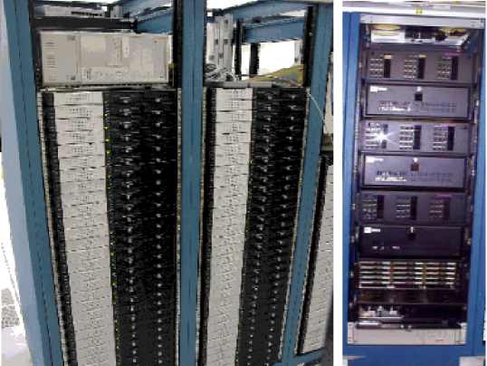
Figure 2: The Parallel Distributed Systems Facility (PDSF) serves several major research groups. It schedules jobs across $\sim 400$ nodes with a fair-sharing queuing system. Images courtesy of NERSC and PDSF.

6 QUESTII Image Processing - Some Details

The steps described above had to be modified slightly to accommodate the QUESTII camera that was added to the Palomar Oschin 1.2-m telescope in April, 2003. This camera can be operated in either of two modes, drift-scan and point-and-track. The NEAT group uses the camera in the standard point-and-track mode, while the QUEST group uses it in its drift-scan mode. There are some differences in the processing of the images taken in each mode.

Drift-scanning is an observing mode in which the telescope is pointed to a desired declination and hour angle and then left fixed with respect to the Earth. The sky thus passes over the CCD as it records. The readout of the CCD is synchronized to this sky motion by reading out a row of the CCD and shifting all of the other rows in time with $15\hbox{${}^{\prime\prime}$}$/second. The QUESTII camera has $0.87\hbox{${}^{\prime\prime}$}$ pixels and so clocks out at $15\hbox{${}^{\prime\prime}$}/\mathrm{second}/0.87\hbox{${}^{\prime\prime}$}/\mathrm{pixel}\approx 17~{}\mathrm{pixels}/\mathrm{second}$ at a declination of zero degrees. In a simplified picture, this fixed scan results in just one exposure per observing night. The QUESTII camera has four separate fingers running parallel along near constant lines of RA, a setup that results in four images of each part of the sky observed in a given night. In practice, there are generally several scans taken to cover areas in the sky at different declinations. In addition, calibration scans are taken to generate equivalent dark frames and sky flats.

For the QUEST project the sky observations are taken in either of two filter sets, UBRI and rizz, while the NEAT group has chosen an RG-610 filter, a long-pass filter beginning at $6100$Å. The NEAT group has used unfiltered observations on the previous Palomar camera and at Haleakala. The choice of an RG-610 filter for the NEAT observations with the QUESTII detector would appear non-ideal both for the purposes of the NEAT group, which selected the filter, and for the purposes of the SNfactory. Certainly, if there were no sky, then it would be in the SNfactory’s best interest to conduct the supernova search unfiltered to maximize the number of discovered supernovae. At the same time, however, it is also beneficial to be able to compute magnitudes on a standard filter system for comparison with other SNe observations.

The SNfactory discussed the relative merits of filtered vs. unfiltered observations with the NEAT group and it was determined that the advantages and disadvantages of using a standard filter balanced out. The light lost in dark time was balanced out by the extra light suppressed in bright time. However, the choice to use a low-pass filter like the RG-610 is non-ideal as it eliminates a large fraction of the wavelength range where the Sun is brightest (asteroids are visible through reflected sunlight) while still allowing contamination from sky glow. It does avoid the increased scattered light from the Moon during bright time, but there is an overall loss of sensitivity to search for asteroids. In addition, the long-pass filter results in fringing on the science images from sky lines in the near-infrared. For supernova work, the RG-610 filter choice is similarly inconvenient. While there are reasons one might choose to use a filter in supernova searches–one might give up V-band coverage, where supernova are brighter than in R-band, in order to be on a known filter system such as a Johnson-Cousins R-band–but there is no such useful tradeoff in this case.

That said, the non-optimal sensitivity caused by this filter choice should not cause any significant problems with the search because the improved QE and reduced pixel scale of the new camera yield a net increased in detection sensitivity of $0.7$ magnitudes over the previous NEAT12GEN2 camera discussed in Sec. 5.

Surprisingly, it was found that the new QUESTII RG610-filtered observations yielded few residuals when subtracted against the older unfiltered Palomar images. There are some residuals at the center of stars, likely due to differential sampling of the different PSFs, but there are no obvious cross-filter-related problems. These good cross-filter subtractions seem to indicate that most of the stars used to calculate flux ratios between images were the same color as the galaxies. It is also possible that the galaxies are being slightly over-subtracted to a degree not clearly visible in the subtractions. The reliability of cross-filter subtractions should be investigated further if the SNfactory decides to use them as a standard part of the search program.

7 Search Images

The telescope observing program covers the same fields in the sky as often as possible while assuring full sky coverage from approximately $-40$^∘ to $+40$^∘ in declination (the Haleakala telescope is the main source for regions with declinations $\mathrel{\hbox{\hbox to0.0pt{\hbox{\lower 4.0pt\hbox{$\sim$}}\hss}\hbox{$<$}}}-25$^∘). In ideal conditions, the full usable sky pattern can be repeated in as few as six days, but bad weather and varying moon illuminations make for a more complicated observing pattern that can average out to as long as two weeks between initial and repeat coverage.

However, since there is now a multi-year baseline of images to select from, the SNfactory search pipeline now conducts subtractions against the full seasons-worth of year-old references for a particular field. These images are stacked together in a co-addition that spans the union of the area covered by the reference images. Eventually, a set of super-reference images should be made that maximizes the use of information from both good and bad images to produce an optimal reference tile for each field on the sky. These premade references would reduce processing time and allow all of the reference tiles of interest to be loaded during the season for which they apply.

Once the search images are taken, they are transferred to LBL and processed as described above. These images will then become the reference images for searches when the search returns again to these fields the following year. Once the search images are loaded into the database, a matching program, findmatches.pl, is run to construct lists of matching fields for the reference and search nights. These lists are then used in generating files which describe the image subtractions to be done to look for supernovae. This matching takes about $30$ minutes, comparing all of the images for a night to all of the images from the previous year and generating an appropriate list of subtractions to be done. As of the summer of 2004, the pipeline performs subtractions against reference images taken $360\pm 240$ days before to the search images.

8 Image Differencing: Subtraction

The SNfactory has adapted the SQL database framework and image subtraction and scanning IDL code developed by the SCP to the specific needs of a low-redshift, large-area search. Chapter 3 chapter presents a detailed description of the image subtraction techniques employed and improved upon by the SNfactory.

9 Object Identification and Scoring

After the subtraction is complete, an automated scanning program takes the final result of the image subtraction and looks for remaining objects. A variety of cuts are applied to the objects found in the subtraction to eliminate cosmic rays, asteroids, and detector artifacts such as hot pixels, bad columns, stray light, and an array of other effects that have been observed over the years. These cuts are based on “scores” that describe features of each candidate as outlined below.

Candidate Scores

For each object found in the subtracted image, a set of quantitative scores is calculated by the automated scanning program. Table 1 shows a list of these scores while Table 2 shows the thresholds used by the SNfactory.

APSIG	The signal-to-noise in the candidate aperture (ap.)
PERINC	The percent increase from REF$\rightarrow$NEW in the candidate ap.
PCYGSIG	Normalized: flux in 2*FWHM ap. - flux in 0.7*FHWM ap.
MAXPIXSIG	Limit on maximum pixel value (unused)
MXY	The X-Y moment of the candidate
FWX	The FWHM of the candidate in X
FWY	The FWHM of the candidate in Y
NEIGHBORDIST	Distance to the nearest object in the REF
NEIGHBORMAG	Magnitude of the nearest object in the REF
MAG	Magnitude of the candidate
THETA	Angle between the candidate and nearest object in the REF
NEW1SIG	Signal-to-noise of candidate in NEW1
NEW2SIG	Signal-to-noise of candidate in NEW2
SUB1SIG	Signal-to-noise of candidate in SUB1
SUB2SIG	Signal-to-noise of candidate in SUB2
SUB2MINSUB1	Weighted signal-to-noise difference between SUB1 and SUB2
DSUB1SUB2	Difference in pixel coordinates between SUB1 and SUB2
HOLEINREF	Signal-to-noise in aperture in the REF
BIGAPRATIO	Ratio of larger aperture to smaller aperture of candidate
OFFSET	Correlation with neighbor distance and angle on subtraction
RELFWX	Candidate FWHM in X divided by NEW image FWHM in X
RELFWY	Candidate FWHM in Y divided by NEW image FWHM in Y

Table 1: The quantitative scores used by the automated scanning program to assist in identification of likely supernovae.

Score	Minimum	Maximum
APSIG	5	–
PERINC	25%	–
PCYGSIG	0	–
MAXPIXSIG	–	–
MXY	-50	+50
FWX	1.01	7.0
FWY	1.01	7.0
NEIGHBORDIST	0.5	–
NEIGHBORMAG	–	–
MAG	–	–
THETA	–	–
NEW1SIG	3.5	–
NEW2SIG	3.5	–
SUB1SIG	3.5	–
SUB2SIG	3.5	–
SUB2MINSUB1	-2.5	+2.5
DSUB1SUB2	–	0.5
HOLEINREF	-5.0	–
BIGAPRATIO	–	5.0
OFFSET	–	–
RELFWX	–	–
RELFWY	–	–

Table 2: The thresholds for the scores described in Table 1 as set for the Palomar 1.2-m NEAT12GEN2 detector. Each detector has a separate set of thresholds tuned to eliminate the characteristic false candidates on subtractions from that detector.

These scores are kept as single floating point numbers and can be restricted by both minimum and maximum limits. For some scores a minimum restriction is obvious, as for APSIG and PERINC. For others, for example SUB2MINSUB1 and DSUB1SUB2, the minimum possible value of 0 is a good score; for these scores, only a maximum restriction is used. Table 2 shows the final thresholds used for the scores in Table 1 for the NEAT12GEN2 detector. These scores were determined in consultation with the experienced SNfactory scanners (see Sec. 10) to eliminate non-supernova objects detected in the subtractions in favor of the good supernova candidates. Eventually, the optimal thresholds for these scores should be determined by analyzing the quantitative score parameter space occupied by the real supernovae as compared with the non-supernova objects.

More on Scores Added for the SNfactory

To reduce the number of objects to be scanned by a person, a number of scores were added to the already existing list from the SCP subtraction code: HOLEINREF, BIGAPRATIO, OFFSET, RELFWX, and RELFWY.

HOLEINREF was created to discriminate against depressed regions in the reference image that would naturally lead to false positive regions in the subtraction. This score calculates the signal-to-noise ratio in a 1-pixel aperture at the candidate location. It is designed more to eliminate defects and bad pixels than to discard large-scale depressions. But, as the large-scale negative regions on the reference will not lead directly to a point-source-like object on the subtraction, it is more important to deal with the pixel-level defects.

RELFWX and RELFWY were designed to ensure that the object shape in the subtraction is at least roughly consistent with point-sources in the NEW image. These scores are particularly helpful in eliminating artifacts in the subtraction due to bad or elevated columns in the NEW or REF images. Similarly, the MXY score detects objects with X-Y moments that would indicate a significant distortion. It is not weighted by the characteristic MXY of the NEW image, although perhaps such a RELMXY score could be considered in future improvements.

A table is kept in the PostgreSQL database that stores all of these scores for every object found on every subtraction. This table allows the SNfactory to search the parameter space defined by these scores to distinguish supernova candidates from non-supernova objects and subtraction or detector artifacts. Currently the scores are implemented independently, but it is likely that there are more complicated combinations of scores that might prove more useful in discriminating good candidate supernovae. For example, the HOLEINREF score could be used in conjunction with the APSIG score. As the HOLEINREF score is designed to eliminate objects that result from negative regions in the REF, one could calculate the contribution that the negative amount measured by the HOLEINREF score would have on the APSIG and increase the APSIG cut by that amount. In this way, an object with an APSIG of 100 could still be accepted even if its HOLEINREF score were -5 (currently excluded by the default score cuts).

HOLEINREF is an important score and is particularly helpful in quantifying the contribution to the subtracted images from negative regions in the REF. Because of the display of the images, human scanners often have difficulty determining the extent of a negative region in the REF. For this reason, there is an inverted grey-scale display of the region around a candidate in the REF image shown in the tiles view (see Fig.7).

RELFWX and RELFWY were very effective in eliminating objects obviously inconsistent with a PSF. Specifically, false objects from unmasked bad columns typically have a non-symmetric shape elongated along the column. Cosmic rays have generally been eliminated by the multiple NEW images, but low pixels in the REF that are not caught by HOLEINREF can still persist and result in objects in the subtraction. However, these objects, are narrower than the characteristic PSF score and so can be eliminated by cuts on RELFWX and RELFWY.

All of the tasks detailed up to this point are fully automated and run daily with minimal human supervision. Figs. 3, 4, 5, and 6 show the processing statistics for 2002 and 2003.

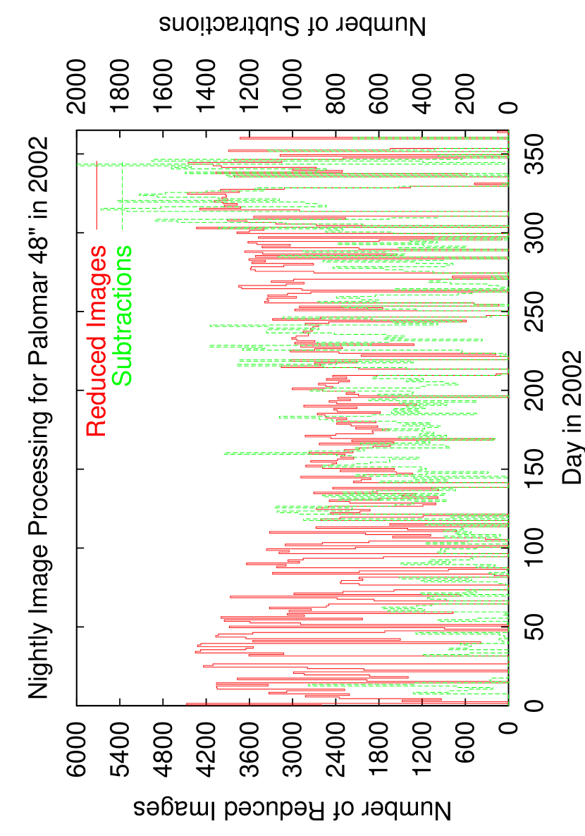
Figure 3: The nightly image processing numbers for the Palomar 48” Oschin telescope for 2002. The solid (red) line denotes the number of images (measured in individual CCD amplifiers) and the dotted (green) line gives the number of subtractions completed for the night.

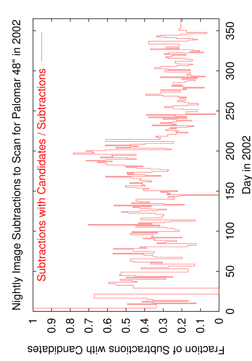
Figure 4: The fraction of the subtractions (see Fig. 3) that had to be scanned by human eye in 2002 given the automatic scanning score cuts in use at the time.

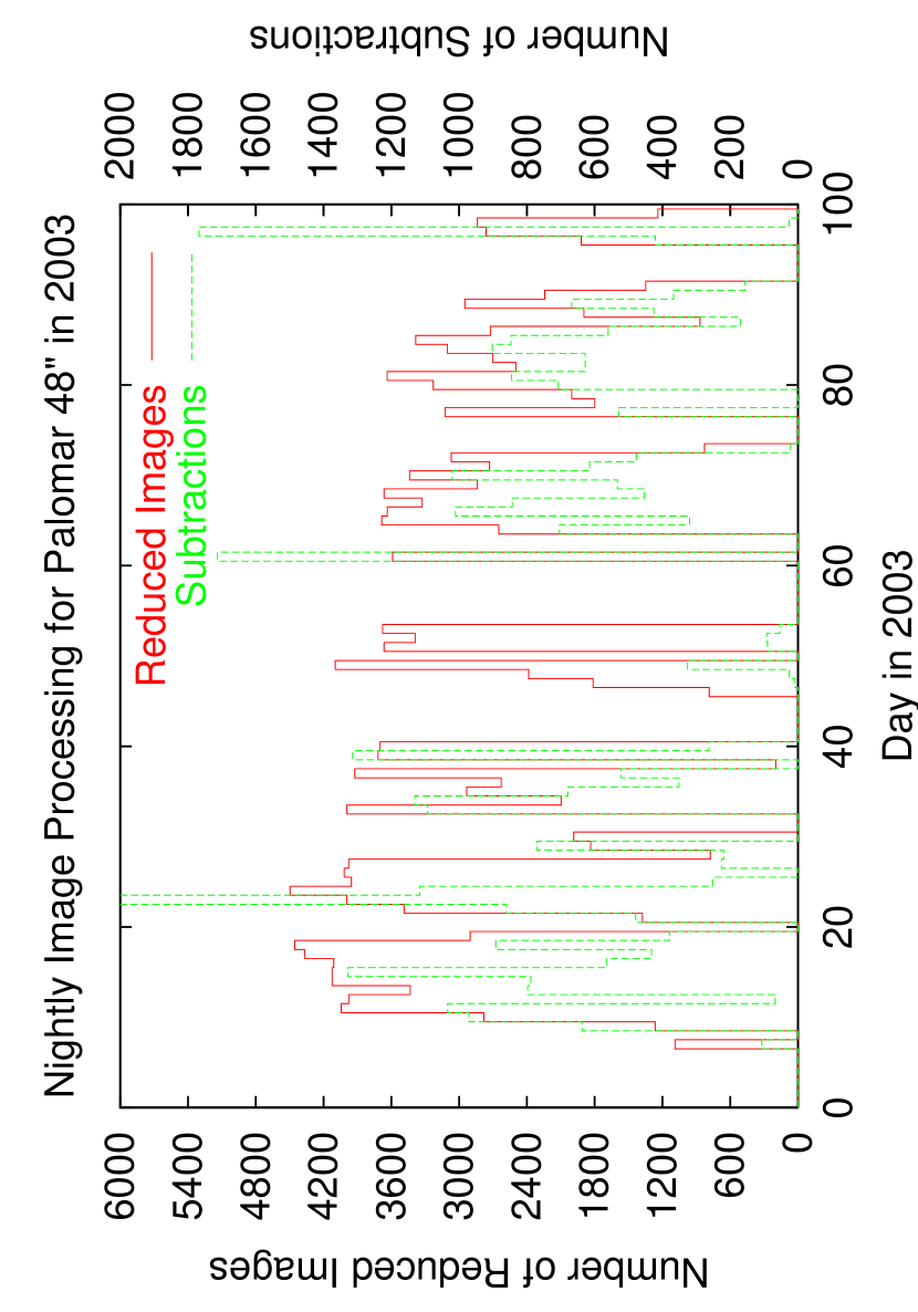
Figure 5: The nightly image processing numbers for the Palomar 48” Oschin telescope for 2003. The solid (red) line denotes the number of images (measured in individual CCD amplifiers) and the dotted (green) line gives the number of subtractions completed for the night.

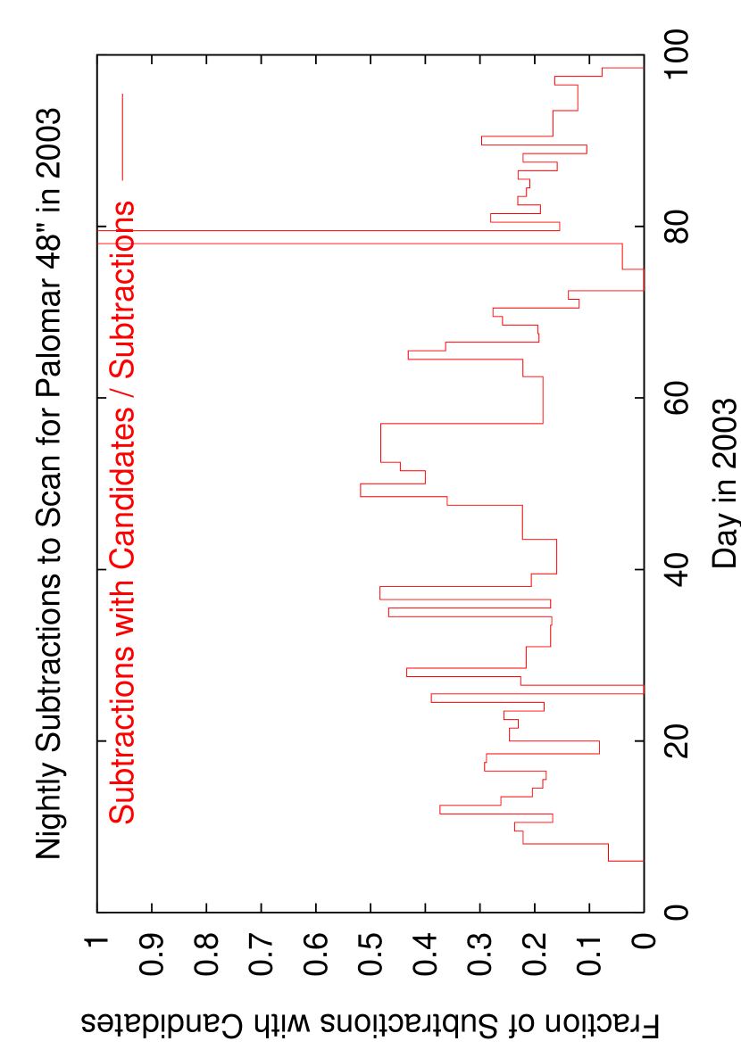
Figure 6: The fraction of the subtractions (see Fig. 5) that had to be scanned by human eye in 2003 given the automatic scanning score cuts in use at the time.

10 Human Scanning of Supernova Candidates

After the pipeline has automatically processed the search images, run the subtractions, and classified the new objects found in the subtractions, a human eye makes the final decision regarding candidate supernovae. The automated scanning program passes a list of flagged candidates on to a human scanner who then looks at the subtracted, search, and reference images and decides whether or not each computer-flagged candidate is a real, variable object.

Scanners learn to search for supernovae in the SNfactory data stream by examining the almost one hundred supernovae already found by the search pipeline to learn what supernovae look like in the SNfactory subtractions. LBL staff scientists and postdoctoral researches who have already been trained to scan for supernovae for the high-redshift SCP searches can rapidly adjust to scanning for nearby supernovae.

The SNfactory search pipeline ran with a very conservative set of cuts in 2002 and $20$–$40$% of the successful subtractions for each night had to be scanned by a person. During the Spring 2002 academic semester, a team of six undergraduates scanned the subtracted images. By the end of the semester, their training and experience enabled them to keep up with the rate of subtractions when they each worked a few hours a week.

However, many of the supernovae discovered in Spring 2003 were found using very restrictive cuts such that only a dozen or so images a night would have had to be scanned. These more aggressive cuts were instituted after the undergraduates stopped working for the semester and after the number of subtractions attempted and completed was increased by considering matching reference and search images from larger date ranges in the database. It is currently possible to the meet the scanning burden with $3$–$6$ staff scientists and postdoctoral researchers working less than an hour per day.

1 Scanning Interface

The scanning interface used by the SNfactory search (see Fig. 7) represents a mild evolution from the software used by the SCP. Each subtraction is first seen whole, with objects and good candidates marked. Then the user looks at each candidate individually in a “tiles” view. A variety of options, in the form of buttons in the graphical user interface, were added for the SNfactory search to aid the scanner in classifying candidates. For example, there is a button on the tiles view window to generate a lightcurve for the RA and Dec of the current candidate from all available NEAT images; another to retrieve an image of that region of the sky from the Digitized Sky Survey (Space Telescope Science Institute 2003); and a number of different fields and toggles to enhance the display of the candidate.

To check for known causes of variable objects that are not supernovae, a number of cross-checks are performed:

1. Check for known asteroids (MPEC Minor Object Catalog).

2. Check for classification of object as star/galaxy (POSS/APM catalogs).

3. Check year-old references to spot long-term variable objects (variable stars, novae, i.e. not supernovae) on both archived NEAT images and DSS/POSS images.

4. Examine automatically generated lightcurve of candidate.

Once a determination is made that a candidate is a possible supernova, the scanner presses the “Keep” button and adds comments and an assessment of the candidate. The candidate is then automatically entered into the database of candidates. Currently a human supervisor checks the list of new candidates and submits promising ones for follow-up, but this process can be easily automated once all of the SNfactory scanners are thoroughly trained.

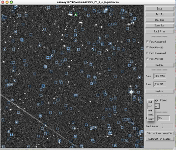
(1) REF

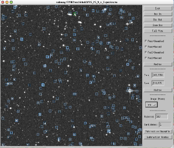
(2) NEW

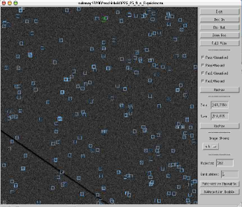
(3) SUB

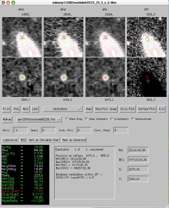
(4) Tiles

Figure 7: The scanning software used to check subtractions flagged by the SNfactory automated system as having candidates of interest. Shown here are the (a) reference images, (b) new images, (c) subtracted images, and (d) the close-up “tiles” view for SN 2002cx.

11 Confirmation Image

Promising candidates are automatically submitted to the NEAT target list for the next night of observation. The current turn-around time from the search image being taken to the candidate being submitted for confirmation is 2 days. This time lag will be decreased to just 1 day, i.e. the next night after the search image was taken, by later in 2004 by submitting subtractions during a night as soon as each full search triplet is available. Once the potentially confirming data is transferred from the telescope, the same region of sky is checked to verify that the variable object is still there.

1 Confirmation Spectrum

To make a final determination that an object under consideration is indeed a supernova, it is necessary to take a confirmation spectrum. For a supernova observed photometrically with a 1-m telescope, spectroscopic observations can be obtained with a 2- to 3-m class telescope. Thus, the UH 2.2-m telescope with the new SNIFS instrument is a good follow-up resource to study SNe discovered with the 1.2-m telescopes used by the NEAT project.

Using the spectra of a number of well-studied SNe, templates of characteristic SNe can be constructed at a variety of times, or epochs, after explosion. These spectral templates at different epochs help determine the type of a SN (Type I a/b/c, or Type II Linear/Plateau/narrow/b + 1987A). At the simplest level, Type I and Type II supernovae are distinguished by the absence or presence of hydrogen lines in their spectra (See Sec. 1). The sub-classes are determined by both lightcurve behavior and spectral features. Spectroscopic and photometric observations will be combined to determine a type for all of the SNe observed as part of the SNfactory program. An early and accurate classification of each SN candidate will be important in focusing the SNfactory follow-up resources on the SNe Ia of interest.

2 Report Discovery

During the prototype search run, after obtaining a sufficient number of images of a candidate that revealed it to exhibit behavior characteristic of a supernova, an IAU circular was submitted to report the discovery of this candidate as an apparent supernova.

A spectral confirmation was not always possible during the prototype search. The SNfactory is grateful to the community for their efforts to spectroscopically observe and determine the types of the SNe discovered by the prototype search pipeline. Now that the SNIFS instrument is installed and operational on the Hawaii 2.2-m telescope, supernovae are distributed within the Palomar Consortium and will be confirmed internally using SNIFS. Spectroscopic observations of the candidate will be conducted to confirm that observed candidates are supernovae and to determine supernova types.

12 Supernovae found to date by this method

Eighty-three new supernovae have been found and accepted by the International Astronomical Union (IAU) using the techniques described above (see Chapter 4). See Tables 2 & 3 for the IAU designations for these supernovae. An additional 17 SNe were found as part of the search but were first reported in the IAU circulars by other groups.

13 Acknowledgements

This research has made use of the NASA/IPAC Extragalactic Database (NED), which is operated by the Jet Propulsion Laboratory, California Institute of Technology, under contract with the National Aeronautics and Space Administration.

Chapter 3 Image Differencing to Find Supernovae: Subtractions

Almost a decade of work has gone into the image differencing, or subtraction, software used by the SNfactory to search for supernovae. The same software used by the Supernova Cosmology Project (SCP) to search for intermediate-redshift ($0.1\geq z\geq 0.5$) and high-redshift ($z\geq 0.5$) supernovae is used by the SNfactory to search for nearby (z $\leq 0.1$) supernovae. This software, DeepIDL, is currently IDL-based, with some externally-called C routines, and is continually being improved and rewritten. This chapter provides an outline of the subtraction process and describes some of the specific changes and improvements that were added to the subtraction software for the SNfactory automated search pipeline. See Kim (1999) for a description of the full SCP subtraction code used in the original SCP supernova searches.

The subtraction software takes a lists of images for a given search field and separately registers (aligns) each of the images to a common reference system. The images to be used as a reference, REF, are then added together after they have all been shifted to line up with each other. The list of images to be searched is split into two parts, NEW1 and NEW2, so that there can be two search images to run checks to make sure a possible candidate isn’t an asteroid or cosmic ray. The variations in seeing between the co-added images are matched through a convolution kernel. The co-added REF image is subtracted from the NEW=NEW1+NEW2 image. Objects found in this SUB=NEW-REF image are then ranked using the SUB image as well as individual subtractions from the separate NEW1 and NEW2 co-additions: SUB1=NEW1-REF and SUB2=NEW2-REF. The objects whose scores pass predefined thresholds (see Sec. 9) are then passed on to be checked. This subtraction process consists of many complicated steps but the framework can be described simply.

1 Image Database and Lists

With millions of images in the SNfactory archive, it is important to have an efficient, well-organized database to keep track of all images that overlap with a given field on the sky. The images table in SNfactory database stores the minimum and maximum values of RA and Dec for each image. These coordinates are always stored in B1950 coordinates for ease of searching. To match to a given field on the sky, these minimum and maximum RA and Dec values are compared against the corners of the field to match and all images that overlap with the field by at least a specified amount, generally $50$% of the area of the reference system image, are returned. These images are then added to a list of matching images for a given field on the sky.

2 Quality Control and Image Registration

An image quality analysis program, subng_reduce_and_vet.pro, is then run on the list of matching images determined above. This analysis routine requires that each image can be successfully processed by the basic image reduction software, freduceimage2.pro and that a minimum of 75 stars from the USNO A1.0 catalog (Monet et al. 1996) are found on the image. Since the NEAT4GEN2 and NEAT12GEN2 images are relatively large, $30\hbox{${}^{\prime}$}\times 30\hbox{${}^{\prime}$}$, there are still plenty of stars on any given field. Even the smaller QUESTII CCDs ($34\hbox{${}^{\prime}$}~{}\times~{}8\hbox{${}^{\prime}$}$) still typically have $>75$ USNO A1.0 stars in each frame.

In addition to passing individual quality controls, subng_reduce_and_vet.pro requires that images must also be successfully matched to the reference frame of the subtraction. The reference frame for the subtraction is generally chosen to be the first new search image that passes the initial image-quality cuts. All of the images for the subtraction must be moved to a common frame and it reduces the uncertainties introduced by the transformation to make the common frame one of the images in the subtraction so that the images can be matched directly to the objects on that image rather than on an abstract sky space. The process of matching an image to another image involves taking the coordinates of all point-sources on each image, sorting them by brightness, taking the top 300 hundred objects and producing a transformation between the object lists. This preliminary match is then refined using ftranscorrect2.pro until the desired transformation tolerance is reached. The overall matching between images is handled using the IDL routines called by ftransimages2.pro.

Images with good transformations to the reference system image are kept and stored in a text file to be passed on to the subtraction software, subng.pro. Fig. 1 shows such a subtraction file for the discovery of SN 2002cx. Rejecting images that fail basic image processing and transformation calculations was a key quality-control device for generating the thousands of successful subtractions a night necessary for operation of the SNfactory search pipeline.

REF
apr232002oschinbd51226.fts
apr232002oschinbd54403.fts
apr232002oschinbd61415.fts

NEW1
may122002oschinbd43225.fts
may122002oschinbd50211.fts

NEW2
may122002oschinbd53211.fts

Figure 1: An example of the file list that it sent to the IDL program subng.pro to determine the images to co-add and subtract (see Fig. 2). This particular file lists the images used for the discovery subtraction for SN 2002cx.

subng, $  ’/home/users/wwoodvas/images/20020512p/subdir/submay122002oschinbd43225_25_9_s_6’, $  imgdir=’/auto/snfactry2/images/snfactory’ , tmpdir=’/scratch/wwoodvas/’ , $  snset=’S2002’ , convmatchalg=6 , dilate = 30, /linear, /noreject , $  /noupdate , /DONTSHIPTOMASTERSITE , /simplemaskscantng, ’submay122002oschinbd43225_25_9_s_6’, /autoscan, defaults=’neat’shipinterestingtomastersite, ’submay122002oschinbd43225_25_9_s_6’EXIT

Figure 2: An example of a command file used to run the IDL subtraction program subng.pro, the automatic scanning program scantng.pro, and a final program that uploads interesting subtractions to be scanned shipinterestingtomastersite.pro. The final EXIT line exits the IDL session.

3 Image Masking

Even in the best of conditions, images often have non-linear and non-astrophysical features that need to masked out from the subtraction to avoid generating spurious candidates. The two most common such features are the non-linear response of the CCD as the signal approaches saturation and blooming spikes from saturated stars. See Fig. 3 for examples of these problems.

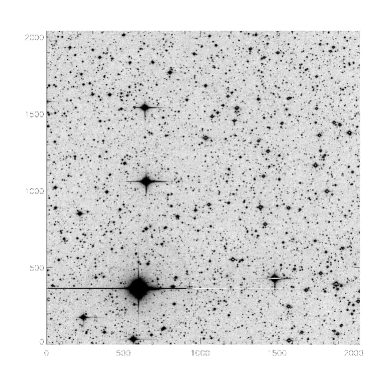
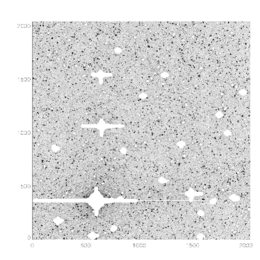
Figure 3: Saturated stars do not subtract cleanly and need to masked to avoid spurious candidates in a subtraction. Note the halos and spikes around the bright stars in the original image shown on the left. Also note that sometimes saturation leads to wrap-around or reflection in the value from the CCD and turns a saturated positive (black) region negative (white) (e.g. the star in the lower-right quadrant). The masked image on the right shows the result of multiplying the original image by the mask generated by makemask.pro.

The very brightest saturated stars affect significant portions of the image, while fainter saturated stars only affect their immediate surroundings. Sometimes the center of a saturated star will look negative, as in the case of some of the stars on the right half of the left-hand image in Fig. 3. It is very important to mask these stars as any negative regions in a reference image will immediately show up in a subtraction as positive objects.

1 Saturated Stars

Saturation occurs in these images because of the large dynamic range of the magnitudes of stars in the field and the nature of the CCD detector. A CCD is a piece of silicon divided into typically a few million cells. Each cell, or pixel, converts incoming photons into electrons. When the CCD is read out, the electrons in each row are shuffled off cell-by-cell and read out by the amplifier. In the case of a linear relationship between the number of photons received and electrons generated, one has a good measure of the original signal.

However, this linearity can only be maintained up to a certain number of electrons in a given pixel. Past this point the response becomes non-linear and the signal is saturated. Saturation can start to be a problem for more than just the immediate saturated pixel because eventually the walls dividing the CCD pixels can no longer contain the accumulated electrons. The electrons leak out from the original pixel and create saturated columns, or readout spikes, extending from the saturated pixel. The star in the lower left corner of the image in Fig. 3 shows this effect clearly.

2 Blooming Spikes, Diffraction Spikes, and Bad Columns

The spikes from saturated stars are a possible source of false candidates as they extend for hundreds of pixels across the image. Bright stars generate readout spikes along the readout column and generate diffraction spikes from the struts, or “spiders”, holding up the secondary mirror or prime focus cage. Because the NEAT (and many other) detectors are aligned so that north is perpendicular to a CCD edge and the spiders are similarly aligned north-south and east-west, the diffraction spikes appear perpendicular to the readout spikes. If the readout spikes weren’t there one should see another pair of diffraction spikes. For many saturated stars, the readout spikes are brighter, but in Fig. 3 one can see that the bright star in the upper-left has relatively symmetric spikes. These are likely predominantly due to diffraction spikes.

As one moves away from the star, the counts in the spikes are often no longer above the saturation level themselves and can only be determined by tracing out the line from the saturated star or by looking for contiguous line segments in a given row.

Both approaches to masking are used in the image masking code makemask.pro. Often fisofind2.pro will find the bulk of the blooming spikes near the star and the object masking from Sec. 1 will take care of those parts.

The full extension of the spikes is dealt with by specialized code that scans the image row-by-row and then column-by-column and traces out line segments. For each row or column the program finds all pixels $5\sigma$ above the noise for the image and marks them as a bad pixel. It then runs through and creates line segments for each bad pixel. These line segments are joined together if they are within 6 pixels of each other. Then all line segments that are at least 10% of the length of the line are masked. If more than $30\%$ of a line is masked the whole line is then marked as masked.

This approach is very successful at masking strong, solid blooming spikes. It also handles bad columns from transient or permanent electronic problems in the CCD. It does not work as well on fainter spikes that don’t produce solid, contiguous line segments. These often come from the optical diffraction spikes which produce fainter, tapering spikes. As the number of spurious candidates due to other sources is decreased, this is starting to become a significant problem and will be the subject of future investigation.

4 Co-addition

The goal of combining images is to maximize the use of all of the information available in the images while minimizing the noise. Once the transformations for all of the images in a set are calculated, the images are each moved to the common reference frame so that all of the pixels overlapping with the reference field match up. Then statistics can be calculated to determine which pixels should be rejected as possibly being from cosmic rays or other irregularities. Obvious cosmic rays will be separately rejected by the masking algorithms which detect all saturated objects. These masks are passed to the co-addition routine and masked pixels from a particular image are excluded from the calculation of the new pixel values in the co-added image. If all of the images have a given pixel masked that pixel is masked in a global mask for the subtraction.

The REF co-addition is created as a union of the component images, while the NEW1 and NEW2 co-additions are created as the intersection of the respective search images. This guarantees that all of the pixels have all three search images to provide information and track the behavior of objects across the three images. It is generally preferable to use references images from the previous year as it can thus be guaranteed that there will be no supernova light in the reference image. No PSF matching is performed in these co-additions for reasons simplicity and maximizing the signal-to-noise in the pixel values. The REF union co-addition uses the relative noise and zeropoints of the reference images in determining their relative weights in making up the “refsum” image. The NEW1 and NEW2 intersection co-additions are simple, unweighted sums. This unweighted co-addition is appropriate for the NEAT same-night image search triplets, but a more generalized approach could be constructed to more optimally deal with search images taken with differing exposure times or in varying observing conditions.

1 Union Co-addition

Each potential reference image is checked to make sure that a transformation to and from the reference frame is possible and well-determined. Images with little or nor overlap with the nominal reference frame are required to have some path of transformation that connects to the reference frame. This allows images that only overlap by 5–10% with the reference frame to be used. However, in practice a minimum overlap of 50% is requires since it is important to ensure that the transformations are all calculated correctly. Just one bad transformation can significantly affect the co-addition because of the chain of transformations used to combine all of the images.

The overall co-addition is constructed as the union of all of the reference images with the intersection with the reference system image. This maximizes the use of historical images to ensure that the reference image is significantly deeper than the search. This also helps reduce the noise in the subtraction so that the sensitivity is primarily limited by the depth of the NEW search images.

5 Point Spread Function Convolution

From the co-added REF, NEW1, and NEW2 images, the aggregate point-spread-function, or “seeing,” of each co-added image is convolved to that of the worst seeing co-added image using a convolution kernel calculated by subngpsfmatch.pro. The co-addition process itself does not convolve because there is no signal-to-noise benefit. However, this means that the PSF on the co-added images is a combination of the PSF of the constituent images and thus may not being easily approximated by a Gaussian function. For the subtraction steps, the PSF differences between the co-added images need to be matched so that objects that are unchanged in the epochs of observations subtract to zero. If these seeing differences are not accounted for there will be doughnut-like positive and negative shapes in the subtractions that would have a net value of zero. These doughnuts complicate the search for new objects in the subtractions. It is much cleaner to properly match up the PSFs of the image so that objects which are at equal brightness subtract to zero and new object show up consistent with a point source according to the point-spread-function of the co-added image with the worst seeing.

There are a variety of methods available in the current DeepIDL framework to calculate the convolution kernel. Currently several Gaussian functions are used to represent the convolution kernel between any two of the co-added images. In the simplest method, the FWHM of a set of good stars is calculated on each image. The quadrature difference of the Gaussian $\sigma$s corresponding to these FWHMs is then calculated. This difference, $\Delta\sigma$, is then used as the $\sigma$ for the convolution kernel to be applied to the image with the smaller FWHM seeing. The method currently used by the SNfactory applies this approach incrementally by only using a given fraction of the calculated $\Delta\sigma$ in each pass. Four passes with fractions of $[0.5,0.5,0.5,1.0]$ are used. This process is done separately in the $x$ and $y$ dimensions. to more fully model the appropriate kernel. This simple centered-Gaussian approach has the advantage of speed, but it doesn’t do a good job in all cases. A project for the future is to improve the calculation of these convolution kernels to yield cleaner subtractions. This improved convolution should significantly reduce the number of false objects in the subtracted images.

6 Flux Matching of Co-Added Images

No explicit calculation or adjustment is made to the co-added images based on relative exposure times. Instead, the brightness of a selection of stars on each image is used to calculate the appropriate flux ratios to normalize each of the images to the same standard. These stars are picked as the brightest, but not saturated, objects identified as stars by fcatalog2.pro. Applying these ratios to the co-added images, a meaningful subtraction of REF from NEW1, NEW2, and NEW1+NEW2 can be realized. This flux-ratio matching accounts for atmospheric transmission, sky brightness, exposure time, and other factors that influence the sensitivity of an image by comparing fluxes of actual astrophysical objects to generate the desired comparison subtraction which should then have the correct flux for any candidate supernova. The flux ratio is defined with respect to the combined NEW image, so the flux zeropoint is set by NEW zeropoint.

7 Actual Subtraction

All of the above work sets up the final subtraction of the pixel values of the flux-matched REF image from the flux-matched NEW1 and NEW2 images to generate SUB1 and SUB2 images and an overall SUB image. The REF, NEW1, NEW2, and SUB images are the only one saved to disk, as SUB1 and SUB2 can be easily reconstructed from NEW1-REF and NEW2-REF, and the overall subtraction is the main image of interest.

8 MAPS Catalog to reject known stars

In a survey with a limiting depth of $20$–$21$ magnitudes, the significant majority of objects will be stars in our own galaxy. Imperfect subtractions result in residuals about these stars. As these residuals can be the cause of a large number of false detections, the use of a catalog of known stars can allow for the rejection of a majority of false candidates.

The Minnesota Automated Plate Scanner (MAPS) Catalog of the POSS I (Kriessler et al. 1998) is used to obtain a list of known stars. This catalog is from a digitized scan of the first Palomar sky survey (taken with photographic plates using the main search telescope used here, the Palomar 1.2-m). The MAPS project used a neural net to classify objects as either stars or galaxies in both the blue and red filters from the POSS I survey (Odewahn et al. 1992, 1993; Nielsen & Odewahn 1994; Odewahn 1995).

To mask known stars for the SNfactory search subtractions, a list was constructed of objects that were classified as being stars with at least $80\%$ certainty in both filters. This list currently contains $\sim$28 million objects and is stored in a PostgreSQL database, taking up 1.2 GB of disk space on a dual-Pentium III 1 GHz machine with 1 GB of RAM, currently lilys.lbl.gov. The entries are stored as integers as described in Table 1.

Field	Format (32-bit Integer)	Scale factor
RA	Decimal Hours	$\times 3600\times 1000$
Dec	Decimal Degrees	$\times 3600\times 1000$
Mag	Magnitude	$\times 1000$

Table 1: The format of entries stored in the stars_radec table in the apscatalog database. This database is used to retrieve a list of the known stars for a given image and then to generate a mask appropriate to use to eliminate known stars from being selected as possible candidates in a subtraction.

This stars_radec table is indexed with a BTREE index on RA and Dec to allow for quick access. A typical query takes on the order of a few seconds.

An IDL routine, makestarmask.pro, queries the database and transforms the list of RA and Dec coordinates to pixel positions on the given image. The magnitudes returned by the query are then used in setting the size of the circular mask created for each known star. Specifically the diameter, $D$, of the circular mask for each star is calculated using Eq. 1.

$$D=2^{(\mathrm{mag}_{\mathrm{norm}}-\mathrm{mag}[k])/3}\times D_{\mathrm{norm}}$$ (1)

$$D_{\mathrm{norm}}=10~{}\mathrm{pixels}\ ,\ \mathrm{mag}_{\mathrm{norm}}=15.0~{}\mathrm{mag}$$ (2)

This equation works for different telescopes by assuming the telescopes have a similar pixel sampling as determined by their seeing and pixel scale. That is, this masking diameter assumes that a star is the same size in pixels on different images. $D_{\mathrm{norm}}$ is controlled by a keyword argument to the makestarmask.pro code and so can be easily adjusted if optimum parameters are determined for a given telescope.

See Figure 4 for a sample image and corresponding star mask. Notice how the brighter stars are masked out with larger masking circles.

A starmask.pro is generated for each subtraction and is applied to the subtracted image when the image is scanned for objects. It is not used, however, in further steps when calculating the fluxes and other quantities for each candidate. This starmask.pro is saved for future reference during the hand-scanning process.

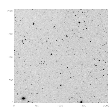
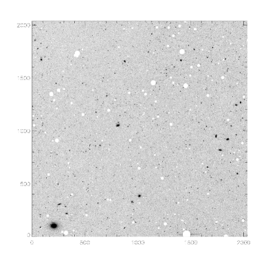
Figure 4: (a) NEAT image ’apr82003oschinbc65109.fts’. (b) The same image with known stars from the APS Catalog (Kriessler et al. 1998) masked out. The bright object in the lower-left corner is a galaxy.

9 Future directions

While the SNfactory automated search pipeline has been very successful, it can still be improved in both efficiency and sensitivity. One desirable improvement would be to construct and keep updated a set of optimum reference images. The second most obvious step to be improved is the convolution matching between the REF, NEW1, and NEW2 images.

A set of super-references would use all of the images available in the NEAT dataset and use the optimum weighting and PSF convolution to maximize the signal-to-noise of the references. Doing this for the tens of thousands of square degrees of sky that the survey covers will require extensive automated quality control and testing to enabled a computer to determine the best way to combine every set of images. It will also require a well-defined set of reference frames. Currently, co-additions to a single reference frame can extend to the edges of the frame, but the astrometric matching is not as well-constrained outside of this region. The geometric scale of both the Palomar 3-CCD camera, QUESTII 112-CCD camera, and the Haleakala 1-CCD camera are relatively flat across each CCD so the transformation solution should be relatively linear and thus hopefully stable to extrapolation and bootstrapping. This linearity and stability of these transformations needs to be verified before building these deep reference images. These super-references would be updated periodically to use new images as they become old enough. This set of optimally-combined images will provide a useful general-purpose data set for a myriad of scientific investigations to maximize the value of this Terabyte-scale survey of the sky.

The simple, yet robust, method currently employed by the SNfactory subtraction code to calculate convolution kernels to match the different PSFs between the REF, NEW1, and NEW2 images could be improved. It currently results in imperfect PSF matching and characteristic residuals in the subtracted image. While the score cuts detailed in Sec. 9, particularly PCYGSIG, RELFWX, and RELFWY, eliminate the majority of these residuals, a cleaner subtraction image would result in fewer objects that need to be checked by a human scanner. An investigation of adapting the Alard and Lupton prescription for a flexible convolution kernel (Alard & Lupton 1998; Alard 2000) was performed, but while some individual subtractions showed excellent convolution kernel matching, in general, an Alard kernel parameterization was not found that was robust enough to result in better subtractions overall. The framework is there in the subtraction code and this work should be pursued further to establish whether or not the Alard convolution kernel technique should be incorporated into the SNfactory search pipeline.

The underlying subtraction and image-processing routines (Chapter 3) for the search pipeline should be completely converted to a non-licensed language. Having to pay for IDL licenses places a significant monetary burden on running a large search on many machines in parallel. Either additional funding should be obtained to cover the IDL licensing costs or the current partially constructed Deeplib C++ framework should be completed to avoid this significant recurring expense. Rob Knop is currently working on developing Deeplib and wrote a new version for the spring and summer HST searches of 2004. Adapting to this new version of Deeplib will involve some changes to the database and auxiliary file structure as well as changes to DeepIDL to ensure backward compatibility with the current IDL framework. Once the new Deeplib reaches a stable release, it would take approximately one month of a qualified person’s time to get subtractions fully integrated and working in the SNfactory pipeline using the new Deeplib once it reaches a stable release.

Chapter 4 Supernovae Found

1 Introduction

As of July 11, 2003, the Nearby SNfactory search pipeline had discovered a total of 99 supernovae. Eight-three of these were found by the SNfactory before other supernova searches. This chapter presents a brief summary of the search efforts and the supernovae found. Sec. 6 presents an analysis of redshifts, discovery magnitudes, and other properties of the supernovae found in this search in the context of a calculation of the rate of nearby SNe Ia.

During 2001 and the early part of 2002, a number of supernovae were found first by other searches and subsequently found by the SNfactory search pipeline. For most of 2001, the search wasn’t actively running so the SNfactory was not the first with the discoveries of supernovae found in this year. In early 2002, the search pipeline was running but the subtractions were not being scanned daily, so the SNfactory discoveries of SN 2002as and SN 2002br were late. After the IAU announcement of SN 2001cp, SN 2001dd, SN 2002as, and SN 2002br, each of these SNe were clearly found in the SNfactory data by the search pipeline in an analysis of older data. They would have been found by the automated search pipeline had it been running when the respective search images were taken.

In the spring of 2002, the search pipeline discovered its first original supernova, SN 2002bk. Eighty-two more original supernovae were discovered over the next year and it was decided that the search pipeline had been proven successful and was ready for full operations once the SNIFS instrument was fully commissioned and operational on the UH 2.2-m.

Sec. 2 details several of the most interesting objects found as part of the prototype SNfactory search: the unusual object S2002-028; the Ia-subtype-breaking SN 2002cx; and the first SN Ia to exhibit clear evidence for hydrogen and a circumstellar medium, SN 2002ic. Sec. 3 presents discovery images and light curves of all of the supernovae observed from 2001 to 2003. Some of the light curves have had their host galaxies subtracted, others have not. These are the rough light curves produced by the automated search pipeline and so include images from all dates available for that region of sky. A simple light-curve based fitting template has been plotted for a selection of the supernovae to illustrate the ability to distinguish supernova type based on the light curve.

2 Interesting Supernovae

1 S2002-028 - An unusual variable object

SNfactory candidate S2002-028 was discovered on images from 21 March 2002. Confirmation images were obtained nine days later on 30 March 2002. The candidate had risen significantly between the two epochs. There was an object present in the reference image which appeared coincident with the brightening object. The 22 February 2002 image did not have the resolution to reveal whether or not the already present object in the 22 February 2002 reference was extended. If it were extended the case would have been stronger for this object being a supernova. Otherwise, the possibility of it being a variable star that flared up in brightness was more of a concern. The Digital Sky Survey plates for the second generation scan contained the field of S2002-028 for both the “Red” and “Blue” plates. An unresolved object was clearly visible in the red plate at the same location as the supernova. No object was apparent in the blue plate at the same location, although there was an object approximately ten arcseconds to the south which was not present in the Red plate. While this blue object was interesting, it was difficult to draw any conclusions regarding this nearby object.

After a request to the NEAT team for special follow-up, this object was observed every other night for over a month with the Samuel Oschin 1.2-m telescope. Over the next week, the candidate continued to rise slowly, consistent with a supernova (see Fig. 1).

However, not having spectroscopic confirmation and being hesitant about releasing a potential dud this early in the prototype search establish the SNfactory as a source of reliable supernova, this candidate was not released the candidate to the International Astronomical Union Circulars (IAUC).

Over the next several months, S2002-028 decayed slowly in brightness. Spectroscopic observations were taken with the Keck telescope and an unusual, unidentified spectrum shown in Fig. 2 was observed. Consultation with several supernova experts (Peter Nugent, Rollin Thomas, and Lifan Wang) yielded no definite identification. The broad features in the spectrum are consistent with differential velocity-broadened lines characteristic of an explosion with a velocity of $\sim 6000$ km/s.

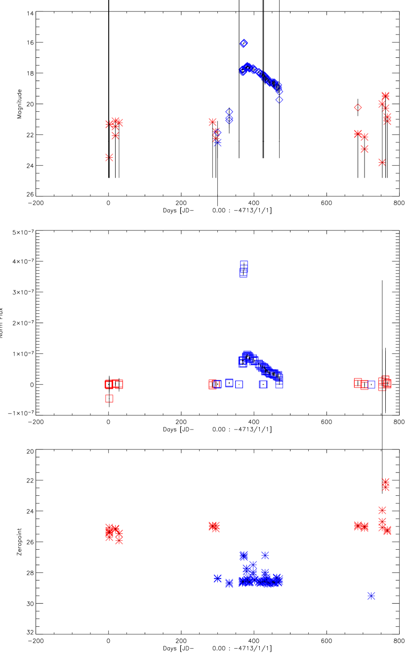
Figure 1: The NEAT unfiltered light curve of S2002-028. Note the very slow decay relative to a SN Ia.

Figure 2: A Keck spectrum of S2002-028. Suggestive broad features are clearly evident, but no match to a known supernova spectrum can be made. The line at $\sim 4500$ Å is an artifact from combining orders in the ESI echelle spectrograph.

2 SN 2002cx

SN 2002cx (Wood-Vasey et al. 2002b) is a stereotype-breaking SNe Ia that does not follow the standard spectroscopic-photometric sequence (Phillips 1993; Hamuy et al. 1995; Riess et al. 1995; Nugent et al. 1995). It is spectroscopically like SN 1991bg, a sub-luminous event, but photometrically like SN 1991T, the classic super-luminous SN Ia (Li et al. 2003). Fig. 3(14) shows the broad, slow-declining profile of this unusual supernova. It is important for the SNfactory to study and understand these unusual objects to provide insight and of avoid contamination of the “normal” SN Ia sample desired for cosmological work.

3 SN 2002ic

SN 2002ic (Wood-Vasey 2002) was discovered in November of 2002 and turned out to be a remarkable SN Ia/IIn hybrid exhibiting the clear silicon absorption feature of SNe Ia before maximum, but then showing strong hydrogen emission  (Hamuy et al. 2003) characteristic of a SN IIn. See Chapter 6 for a discussion of this very interesting supernova.

3 SNfactory Discoveries

The early shake-down efforts in 2001 yielded two supernovae found after others had reported them in the IAUCs: SN 2001cp (see Fig. 3(1)) and SN 2001dd (Fig. 3(3)). Table 1 lists these supernovae along with their discovery magnitudes, redshifts, and host galaxies.

Table 1: Supernovae in the data from 2001.

IAUC Name	SNfactory Name	Discovery Magnitude	Redshift	Comments
SN 2001cp	S2001-165	16.35	0.02240	UGC 10738
SN 2001dd	S2001-099	16.77	0.01969	UGC 11579

1 A successful prototype search pipeline test: 2002–2003

The SNfactory discovered $37$ original supernovae in 2002 (Wood-Vasey et al. 2002a). This was the most ever for the first year of a supernova search. The search continued with great success in 2003 with the discovery of another $46$ original supernovae. In 2003, the search pipeline discovered its first original supernovae using the Haleakala 1.2-m telescope (SN 2003bf, SN 2003bn, SN 2003bp, and SN 2003ey (Wood-Vasey et al. 2003b, f, c, d)). Supernovae had already been found from with the Haleakala telescope that were first discovered by others (SN 2001cp, SN 2002hw, and SN 2002kj (Modjaz & Li 2001; Schwartz & Li 2002; Wood-Vasey et al. 2003e)). By the time the Palomar 3-CCD camera was removed in April, the search pipeline had discovered $41$ supernovae and had reached the target rate of 12 SNe/month. As two-thirds of the spectroscopically-typed supernovae discovered by the early SNfactory efforts have been Type Ia, one can extrapolate that $12$ SNe/month will yield $8$ SNe Ia/month $=96$ SNe Ia/year $\approx 100$ SNe Ia/year. This satisfies the design requirement for the SNfactory automated search pipeline.

Table 2: Supernovae found in 2002.

		Discovery
IAUC Name	SNfactory Name	Magnitude	Redshift	Comments
SN 2002as	S2002-000	18.03	0.02248
SN 2002bk	S2002-006	18.51	0.057
SN 2002br	S2002-058	-9.404	0.034184	disc. mag. in error
SN 2002cq	S2002-054	19.21
SN 2002cx	S2002-070	18.91	0.024
SN 2002cz	S2002-080	18.58
SN 2002da	S2002-078	18.81
SN 2002dg	S2002-087	18.46	0.047
SN 2002dh	S2002-095	15.82	0.013
SN 2002dy	F2002-074	17.78	0.03301
SN 2002ek	F2002-040	19.50
SN 2002el	F2002-048	16.72
SN 2002ep	F2002-039	17.47
SN 2002eq	F2002-041	19.43	0.088
SN 2002ev	F2002-056	18.75
SN 2002ew	F2002-049	17.82	0.03
SN 2002ex	F2002-054	19.12	0.038
SN 2002ez	F2002-043	18.38	0.043
SN 2002fa	F2002-050	19.41	0.06
SN 2002fs	F2002-059	17.44	0.038
SN 2002ft	F2002-062	18.13	0.075
SN 2002fu	F2002-064	19.36	0.091
SN 2002gb	F2002-058	18.89	0.074
SN 2002gd	F2002-070	18.44	0.0085
SN 2002gf	F2002-071	19.19	0.086
SN 2002gg	F2002-069	20.06	0.11
SN 2002gh	F2002-072	19.66
SN 2002gx	F2002-076	18.97
SN 2002gz	F2002-078	18.38	0.085
SN 2002hb	F2002-081	19.13	0.09
SN 2002hf	F2002-087	18.21
SN 2002hj	F2002-089	17.81	0.0236
SN 2002hw	F2002-141	17.24	0.017535
SN 2002ia	F2002-101	19.03	0.072
SN 2002ib	F2002-097	18.24	0.0679
SN 2002ic	F2002-099	18.25	0.0664
SN 2002jf	F2002-104	18.62	0.079
SN 2002jh	F2002-098	18.62	0.048
SN 2002jk	S2002-081	18.46
SN 2002jl	F2002-106	19.50	0.064
SN 2002jp	S2003-152	19.09	0.012362
SN 2002kj	F2002-140	18.51
SN 2002kk	F2002-046	19.42
SN 2002le	S2002-075	19.47
SN 2002lf	S2002-072	19.87

Table 3: Supernovae found in 2003.

		Discovery
IAUC Name	SNfactory Name	Magnitude	Redshift	Comments
SN 2003V	S2003-003	18.50	0.045
SN 2003aa	S2003-113	16.30	0.01013
SN 2003ab	S2003-088	18.17	0.029414
SN 2003ae	S2003-005	17.77
SN 2003af	S2003-011	15.60	0.02
SN 2003ap	S2003-018	16.71	0.03
SN 2003av	S2003-014	19.63	0.14
SN 2003aw	S2003-016	17.72
SN 2003ax	S2003-026	18.52	0.054
SN 2003ay	S2003-025	19.16	0.073
SN 2003bf	S2003-033	17.19	0.034
SN 2003bh	S2003-029	19.93	0.089
SN 2003bi	S2003-030	19.59
SN 2003bn	S2003-073	16.75	0.013
SN 2003bo	S2003-076	19.53
SN 2003bp	S2003-077	18.17	0.019807
SN 2003bs	S2003-080	17.73	0.05
SN 2003bt	S2003-086	16.69	0.027516
SN 2003cc	S2003-112	19.50
SN 2003cd	S2003-111	19.98
SN 2003ce	S2003-094	19.49
SN 2003cf	S2003-115	19.01
SN 2003cj	S2003-138	20.04
SN 2003ck	S2003-129	19.26
SN 2003cl	S2003-147	19.51	0.168301
SN 2003cn	S2003-174	18.34	0.01811
SN 2003co	S2003-120	18.60	0.0824
SN 2003cs	S2003-137	19.36	0.029583
SN 2003ct	S2003-139	19.03	0.046075
SN 2003cu	S2003-145	19.91
SN 2003cv	S2003-156	17.62	0.028
SN 2003cw	S2003-157	20.07
SN 2003cx	S2003-160	19.07	0.037
SN 2003cy	S2003-154	18.96
SN 2003cz	S2003-163	20.16
SN 2003dc	S2003-134	19.33	0.067
SN 2003dd	S2003-133	20.08
SN 2003de	S2003-162	17.22
SN 2003df	S2003-110	20.31
SN 2003di	S2003-116	18.00
SN 2003dj	S2003-126	20.01
SN 2003dk	S2003-150	19.19
SN 2003dm	S2003-167	19.73
SN 2003dn	S2003-164	20.02
SN 2003do	S2003-171	19.91
SN 2003dp	S2003-170	19.98
SN 2003dq	S2003-172	18.91	0.046
SN 2003ee	S2003-149	16.47	0.021
SN 2003ef	S2003-191	17.48
SN 2003eo	S2003-141	20.20
SN 2003ex	S2003-130	19.11
SN 2003ey	S2003-197	18.75	0.065
SN 2003gc	S2003-144	18.00
SN 2003gi	F2003-042	19.18	0.013006
SN 2003gt	F2003-000	18.34	0.015657

4 Current Status of SNfactory search – 2004

The SNfactory search has been proven to yield the necessary number of supernovae to support the SNfactory follow-up program. Operation has begun again as of July, 2004. Data from the QUEST drift-scan program has been integrated into the search pipeline. Using the QUESTII drift-scan data necessitated the incorporation of the more specific coverage pattern of the drift-scan program and the flexibility to reconstruct neighboring segments along the scan strip to maximize overlap in the subtractions. In addition, more robust matching and image quality routines were required to deal with the larger number of marginal quality CCDs on the QUESTII detector. The current plan to use the QUEST drift-scan data is to take references a month prior and then one new image taken on each of two search nights separated by two or three days. Subtractions can be run across different red filters (Johnson R vs. Gunn r) if necessary. In preliminary tests, these cross-filter subtractions have posed no serious difficulties. There are specific tweaks in the matching code to activate this behavior for the QUESTII drift-scan subtractions.

Improvements to the automatic candidates screening will be helpful in reducing the human burden in searching for supernovae. Currently $1$–$5$% of the images need to be checked by hand and $1$% of those have supernovae. This represents a few hours of person-time every day to scan. This is workable, but a more fully automated system would be preferable for better consistency and determinism. Routes toward an improved system include improvements in the suite of candidate scores and an investigation of optimizing the PSF-matching required to compare images taken under different atmospheric and telescopic conditions. Searching for SNe using the QUEST drift-scan data has introduced some benefits and complications in the candidate scoring as the different search nights used in NEW1 and NEW2 have, in general, different PSF shapes. This night-to-night PSF variation reduces artifacts due to improper PSF matching because they are eliminated by the separate requirements in SUB1 and SUB2. However, the effective PSF in the overall NEW image can be harder to match to the REF images. Additionally, over two days between subsequent QUESTII drift-scan search observations, practically everything in the Solar System moves sufficiently to be eliminated by its apparent motion. Only true, stationary astrophysical objects should appear similar enough to be present in the joint subtraction. With its increased area and sensitivity, the new QUESTII camera has the potential to double the SN discovery rate of the SNfactory.

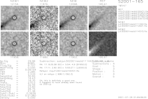
(1) 2001cp

(2) 2001cp

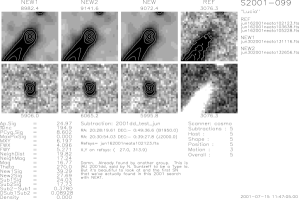
(3) 2001dd

(4) 2001dd

(5) 2002as

(6) 2002as

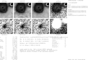
(7) 2002bk

(8) 2002bk

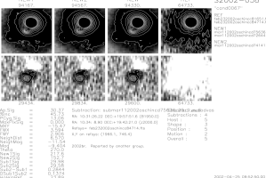
(9) 2002br

(10) 2002br

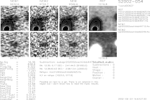
(11) 2002cq

(12) 2002cq

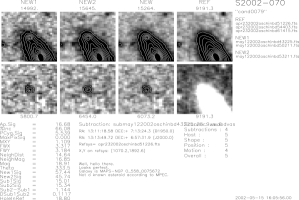
(13) 2002cx

(14) 2002cx

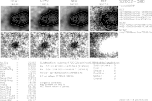
(15) 2002cz

(16) 2002cz

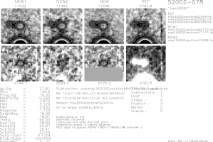
(17) 2002da

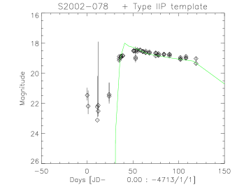
(18) 2002da

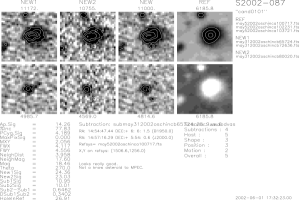
(19) 2002dg

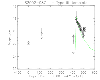
(20) 2002dg

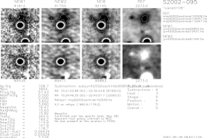
(21) 2002dh

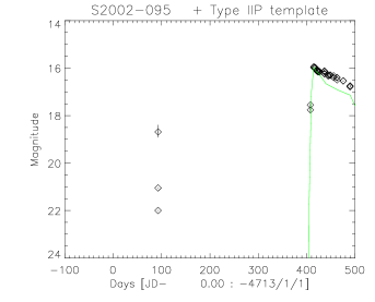
(22) 2002dh

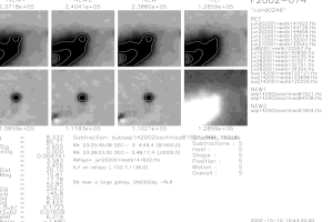
(23) 2002dy

(24) 2002dy

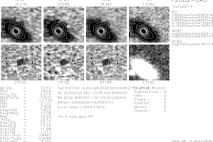
(25) 2002ek

(26) 2002ek

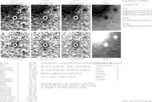
(27) 2002el

(28) 2002el

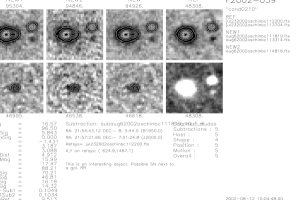
(29) 2002ep

(30) 2002ep

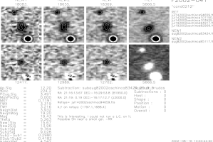
(31) 2002eq

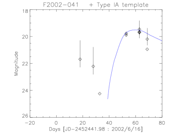
(32) 2002eq

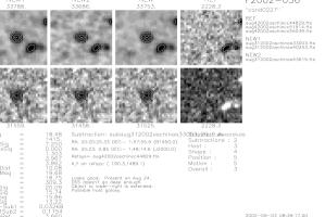
(33) 2002ev

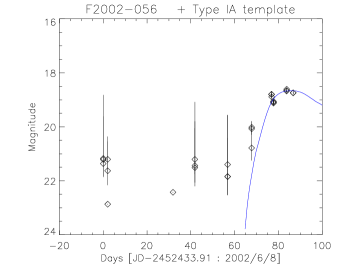
(34) 2002ev

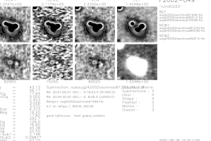
(35) 2002ew

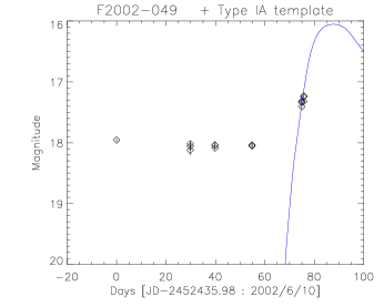
(36) 2002ew

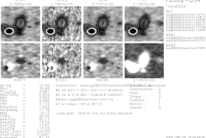
(37) 2002ex

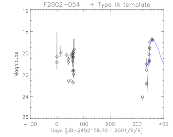
(38) 2002ex

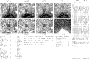
(39) 2002ez

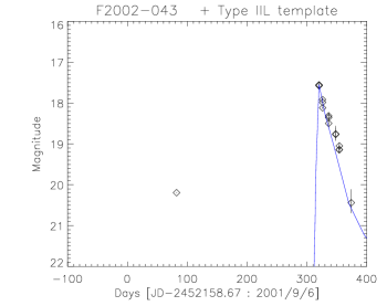
(40) 2002ez

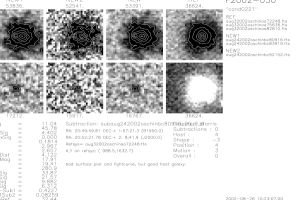
(41) 2002fa

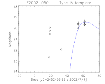
(42) 2002fa

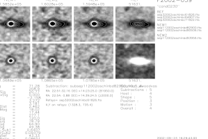
(43) 2002fs

(44) 2002fs

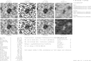
(45) 2002ft

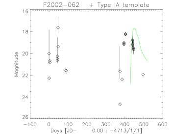
(46) 2002ft

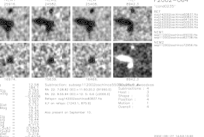
(47) 2002fu

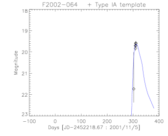
(48) 2002fu

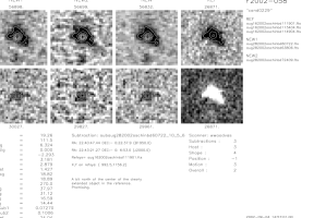
(49) 2002gb

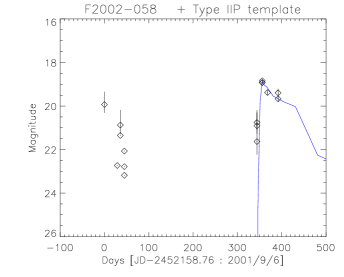
(50) 2002gb

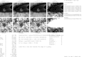
(51) 2002gd

(52) 2002gd

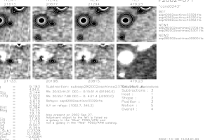
(53) 2002gf

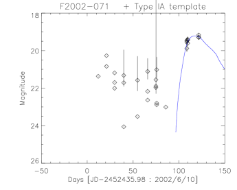
(54) 2002gf

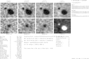
(55) 2002gg

(56) 2002gg

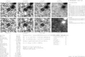
(57) 2002gh

(58) 2002gh

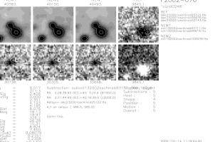
(59) 2002gx

(60) 2002gx

(61) 2002gz

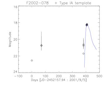
(62) 2002gz

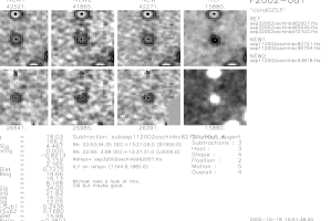
(63) 2002hb

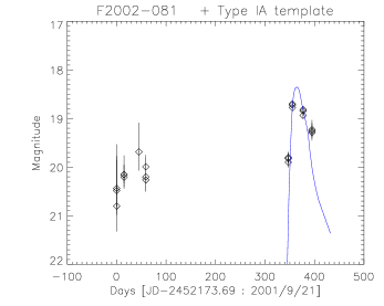
(64) 2002hb

(65) 2002hf

(66) 2002hf

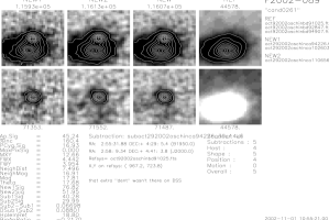
(67) 2002hj

(68) 2002hj

(69) 2002hw

(70) 2002hw

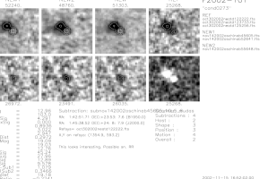
(71) 2002ia

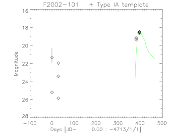
(72) 2002ia

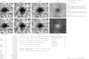
(73) 2002ib

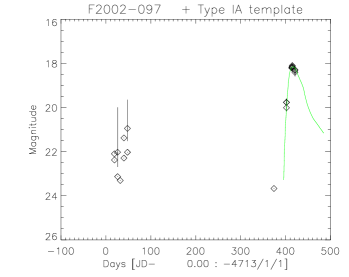
(74) 2002ib

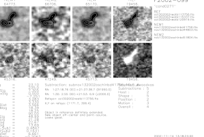
(75) 2002ic

(76) 2002ic

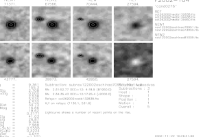
(77) 2002jf

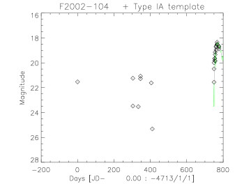
(78) 2002jf

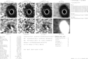
(79) 2002jh

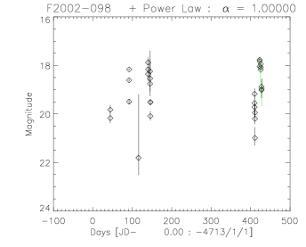
(80) 2002jh

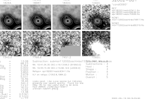
(81) 2002jk

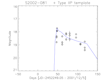
(82) 2002jk

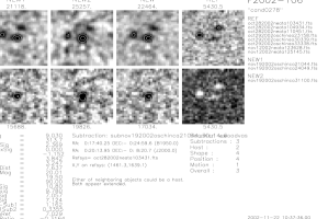
(83) 2002jl

(84) 2002jl

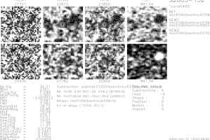
(85) 2002jp

(86) 2002jp

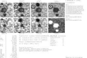
(87) 2002kj

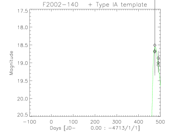
(88) 2002kj

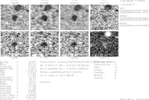
(89) 2002kk

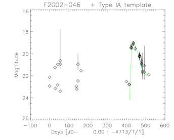
(90) 2002kk

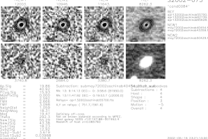
(91) 2002le

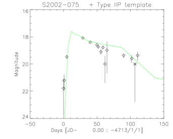
(92) 2002le

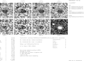
(93) 2002lf

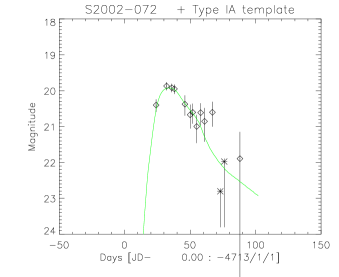
(94) 2002lf

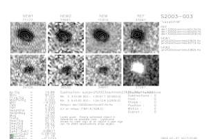
(95) 2003V

(96) 2003V

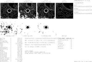
(97) 2003aa

(98) 2003aa

(99) 2003ab

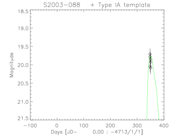
(100) 2003ab

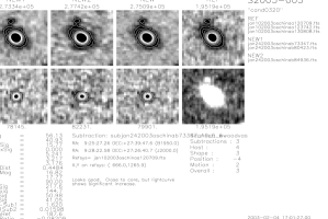
(101) 2003ae

(102) 2003ae

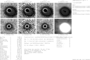
(103) 2003af

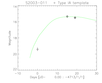
(104) 2003af

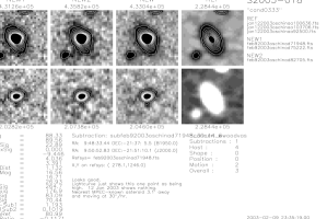
(105) 2003ap

(106) 2003ap

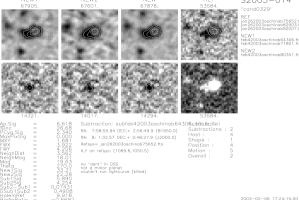
(107) 2003av

(108) 2003av

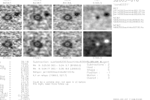
(109) 2003aw

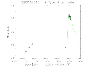
(110) 2003aw. A dwarf nova.

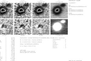
(111) 2003ax

(112) 2003ax. Bad refsys zeropoint.

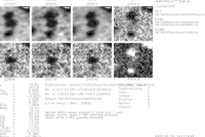
(113) 2003ay

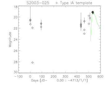
(114) 2003ay

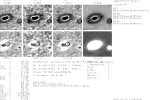
(115) 2003bf

(116) 2003bf

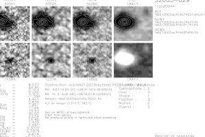
(117) 2003bh

(118) 2003bh

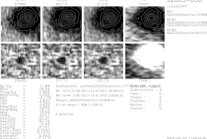
(119) 2003bi

(120) 2003bi

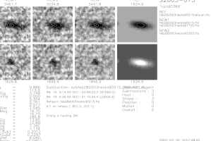
(121) 2003bn

(122) 2003bn

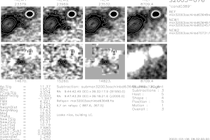
(123) 2003bo

(124) 2003bo

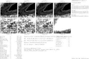
(125) 2003bp

(126) 2003bp

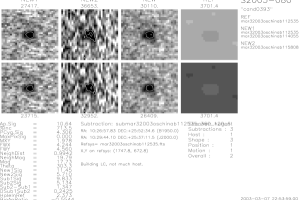
(127) 2003bs

(128) 2003bs

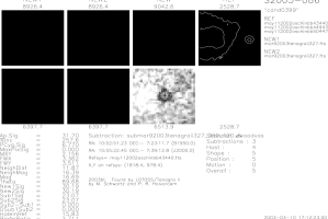
(129) 2003bt

(130) 2003bt

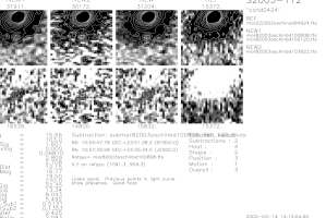
(131) 2003cc

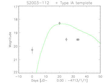
(132) 2003cc

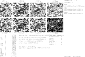
(133) 2003cd

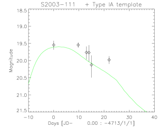
(134) 2003cd

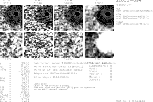
(135) 2003ce

(136) 2003ce

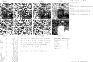
(137) 2003cf

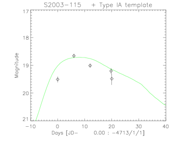
(138) 2003cf

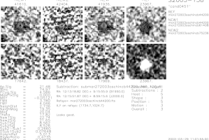
(139) 2003cj

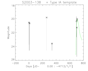
(140) 2003cj

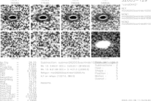
(141) 2003ck

(142) 2003ck

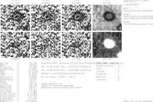
(143) 2003cl

(144) 2003cl

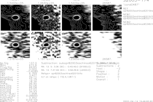
(145) 2003cn

(146) 2003cn

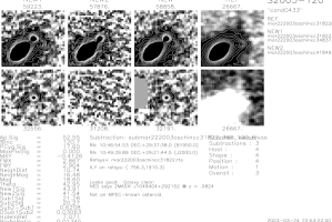
(147) 2003co

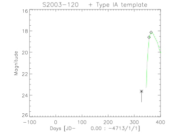
(148) 2003co

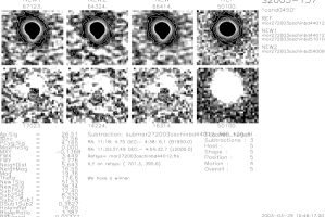
(149) 2003cs

(150) 2003cs

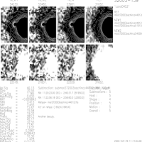
(151) 2003ct

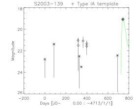
(152) 2003ct

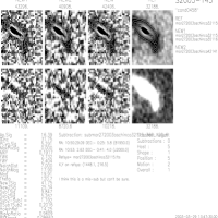
(153) 2003cu

(154) 2003cu

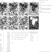
(155) 2003cv

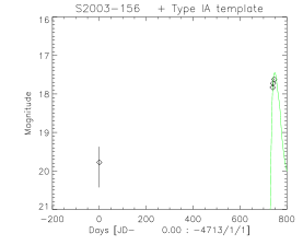
(156) 2003cv

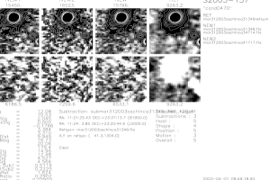
(157) 2003cw

(158) 2003cw

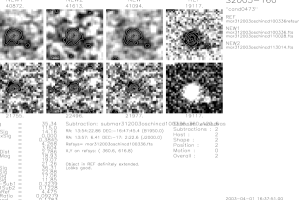
(159) 2003cx

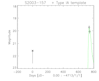
(160) 2003cx

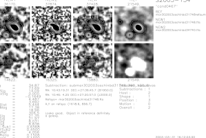
(161) 2003cy

(162) 2003cy

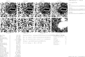
(163) 2003cz

(164) 2003cz

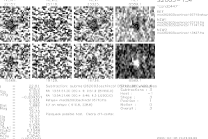
(165) 2003dc

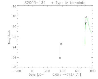
(166) 2003dc

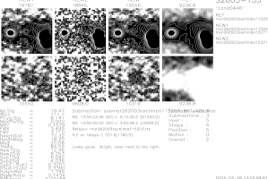
(167) 2003dd

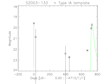
(168) 2003dd

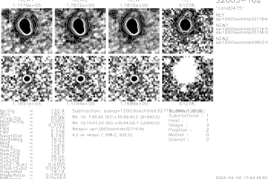
(169) 2003de

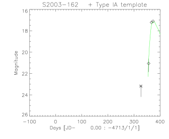
(170) 2003de

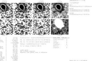
(171) 2003df

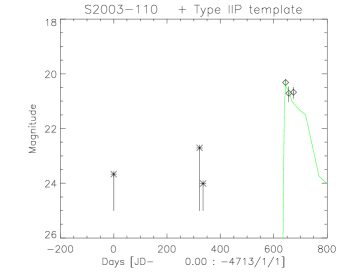
(172) 2003df

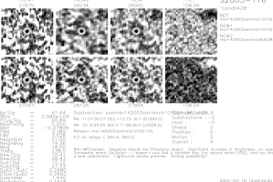
(173) 2003di

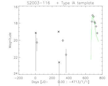
(174) 2003di

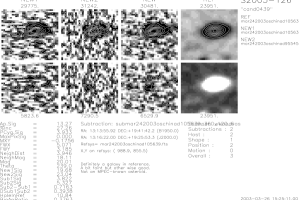
(175) 2003dj

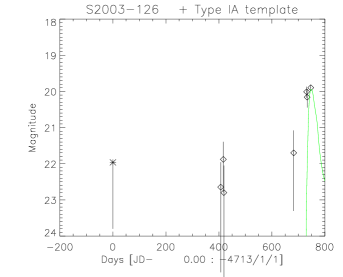
(176) 2003dj

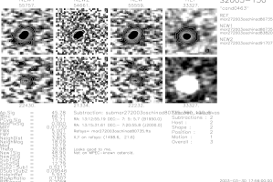
(177) 2003dk

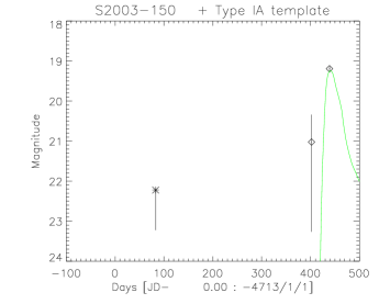
(178) 2003dk

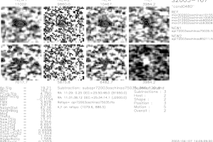
(179) 2003dm

(180) 2003dm

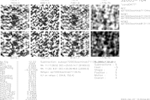
(181) 2003dn

(182) 2003dn

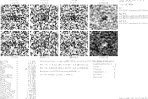
(183) 2003do

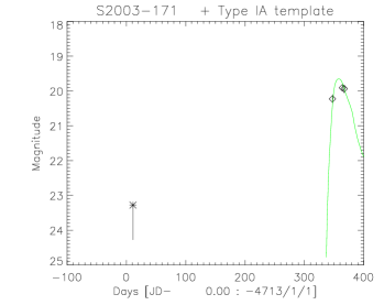
(184) 2003do

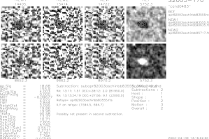
(185) 2003dp

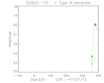
(186) 2003dp

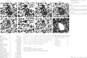
(187) 2003dq

(188) 2003dq

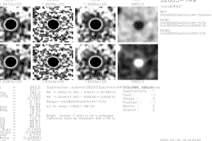
(189) 2003ee

(190) 2003ee

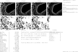
(191) 2003ef

(192) 2003ef

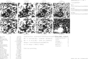
(193) 2003eo

(194) 2003eo

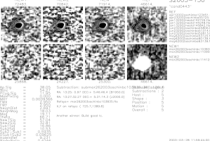
(195) 2003ex

(196) 2003ex

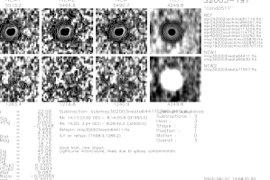
(197) 2003ey

(198) 2003ey

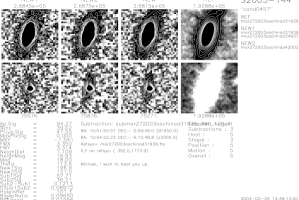
(199) 2003gc

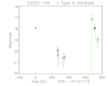
(200) 2003gc

(201) 2003gi

(202) 2003gi

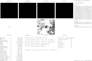
(203) 2003gt

(204) 2003gt

Part 2 Supernova Rates

Chapter 5 Type Ia Supernova Rates from the SNfactory

1 Motivation

Supernovae are a dramatic link to the star formation history (SFH) of galaxies. As discussed in Sec. 3, the SN Ia rate is related to the SFH of the underlying galaxy population. While core-collapse SNe trace the SFH within $\sim 10^{7}$ years of the SN explosion, SNe Ia are connected to the SFH through a delay time dependent on the formation mechanism for SNe Ia (for example, see Madau et al. (1998), Gal-Yam & Maoz (2004), and Strolger et al. (2004)). The delay time between the core-collapse SN rate and the SN Ia rate places constraints on SN Ia progenitor models. More generally, the relationship between the core-collapse and SN Ia rates provides insight into the initial mass fraction, chemical evolution, and star formation rate and history of galaxies (Madau et al. 1998; Maoz & Gal-Yam 2004). The recent interest in SNe Ia for cosmological studies has allowed for and encouraged complementary studies of the rates of SNe Ia to explore galaxy evolution and star formation during the recent expansion history of the Universe (Pain et al. 2002).

2 Introduction

The history of supernova rates has been one of good effort and poor statistics. The central difficulty has lain in the lack of a sample of a large number of supernovae from a well-understood and homogeneous search of the sky.

Fritz Zwicky was a pioneer of supernova studies and contributed the first papers on supernova rates (Zwicky 1938, 1942). He used a 16^′′ Schmidt telescope on Mt. Palomar, California, to study a controlled sample of 3000 galaxies brighter than 15th magnitude. Zwicky (1938) introduced the control-time method of determining supernova rates from a given search program. In its most general form, the control-time method assigns a period of time for which each exposure was sensitive to a supernova explosion. This formalism compresses the variable sensitivities along the rise and fall of a typical supernova into one number. Zwicky assumed a control-time of one month for each observation in the studies mentioned. While convenient and appropriate for the state of knowledge of supernovae in 1938, the difference in light curves between types of supernova can lead to errors in estimation of the supernova rate, a possibility Zwicky considered and then dismissed in the context of his own study. For example, assuming that every supernovae would be of Type I results in an underestimate of the total supernova rate due to the fact that Type II supernovae are intrinsically dimmer and thus fewer are seen in a flux-limited survey.

To conduct an accurate rate estimation, one needs to model the light curves of the supernova expected and then compare the fit of the model to the data obtained. This chapter will present an analysis of the nearby ($z<0.1$) SN Ia rate done in the manner of Zwicky’s original control-time method, a more generalized control-time analysis that fully models the light curves of SNe Ia, and, finally, the preferred solution of using a simulated set of 200 million SNe Ia throughout the search coverage in time and area to directly measure the actual sensitivities of the search images.

At present, the distant supernova rate is better understood than the nearby supernova rate because of the way distant supernova searches are conducted. Searches for high-redshift SNe take deep exposures of a couple of square degrees (or less) of the sky. The volume covered by this exposure samples all galaxies in the region, unlike the nearby, directed supernova searches, which target known (and thus usually brighter) galaxies. The small number of fields and easily calculable control times characteristic of distant supernova searches have allowed the determination of the supernova rate at $z=0.55$ to $\sim 15\%$ (Pain et al. 1996, 2002). The very nearby supernova rate ($z\sim 0.01$) is known to $\sim 30\%$ (Muller et al. 1992; Cappellaro et al. 1997, 1999a), but the nearby supernova rate is only known to $40$–$90\%$ (Hardin et al. 2000; Blanc et al. 2004).

Cappellaro et al. (1997) presented the results of five SN surveys in an attempt to estimate the nearby supernova rate. While the paper did a reasonable job with data at hand, its conclusions were a bit speculative because of the limitations of the searches. Cappellaro et al. (1999a) updated this attempt by focusing purely on the search of Evans (1997) as a consistent, homogeneous sample of supernovae. The greatest limitation of this second paper is that Evans’ search was only of known and generally bright galaxies. As a result, the rate in the general field of space is poorly determined from Evans’ data. This galaxy-selection effect is a common limitation of nearby supernova searches. In contrast, the large-sky survey of the Nearby Supernova Factory (SNfactory; see Part. 1) represents a major improvement in the ability to calculate general supernova rates.

3 Supernova Rates from Supernova Searches

Supernova rates are traditionally expressed in supernova units (SNu), where 1 SNu = 1 supernova / $10^{10}$ $L_{B}\odot$ / century (for example, see Cappellaro & Turatto (1988)), which is loosely speaking one supernova per galaxy per century. This unit is chosen because there is evidence that the supernova rate is proportional to luminosity (Tammann 1970). In this way, the SNu allows one to compare different galaxies in a standard manner. Most supernova searches to date have been directed-galaxy searches and so the SNu has been a way to standardize the known-galaxy supernova rate to the supernova rate in the overall Universe. This chapter presents a determination of the SN Ia rate from a sample of the prototype SNfactory search.

The SNfactory search is an areal search that covers half of the sky without regard to known galaxies (except our own—see Fig. 3 for the typical NEAT coverage). For this reason, this study will quote the SN Ia rate per unit volume. Using a galaxy luminosity density function from the Sloan Digital Sky Survey (Blanton et al. 2003a), the SN Ia rate will be translated to SNu for comparison with other recent studies (Cappellaro et al. 1997, 1999a; Hardin et al. 2000; Pain et al. 2002; Dahlen et al. 2004). The convention used in Pain et al. (2002) will be adopted here with the SN Ia rate expressed per volume denoted by $r_{V}$ and the rate per luminosity denoted by $r_{L}$.

In the case of known-galaxy searches, supernova rates are generally quoted per blue luminosity as galaxy blue luminosity is a measurable quantity believed to be correlated with the supernova rate and available to normalize the rates. It is important to bear in mind, however, that the blue luminosity of a galaxy as a proportion of total luminosity depends on its type (Cappellaro et al. 1999a). In addition, known-galaxy searches are strongly biased toward finding supernovae only in galaxies on the brighter end of the galaxy luminosity function. Fig. 1 shows this effect in the host galaxy luminosity distribution for local supernovae.

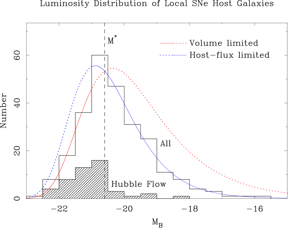
Figure 1: The host galaxy luminosity distribution for local supernovae from the Asiago catalog. The solid line shows the distribution of all galaxies and is consistent with a volume-limited sample for the brightest galaxies and a flux-limited sample for intrinsically fainter galaxies. The shaded histogram shows the luminosities of galaxies in the Hubble flow. Note the sharp cutoff for Hubble-flow galaxies with $M_{B}<M^{\star}$. This cutoff demonstrates the significant bias in the host galaxy source population for Hubble-flow SN searches using known galaxies. The different results expected for volume-limited and galaxy-flux-limited searches are indicated by the “Volume limited” and “Host-flux limited” lines. The “All” histogram indicates the SNe found prior to the SNfactory project and is consistent with a volume limited search for bright galaxies but host-flux limited for fainter galaxies. The SNfactory will conduct an essentially supernova-flux limited survey, which will result in galaxies selected following the “Volume limited” curve (but see Sec. 5). This survey will thus have better representation of galaxies at the faint end of the luminosity function than previous nearby supernova surveys, particularly out in the smooth Hubble flow. (Figure courtesy of Greg Aldering.)

In contrast, a “blind” search, scanning large swathes of sky, provides an excellent opportunity to calculate supernova rates from a much more complete sample of host galaxy luminosity types. The galaxy sample is determined by the area and flux limit for detection of supernovae, rather than the luminosities of the galaxies, as it would be for a known-galaxy search. Because the spread of SN Ia luminosities is much smaller than that of galaxies, and their light curves are well understood, the limiting magnitude at the faint limit of a “blind” search can be determined with relative confidence (but see Sec. 5).

When calculating a supernova rate, the most salient factor is the control time of the search, $T(z)$, or the amount of time the search is sensitive to a supernova as a function of redshift. The control time includes all relevant search efficiencies and observation cadences. To compare with observations, the number of supernovae found as a function of redshift, $N(z)$, is compared to the predicted value given the rate as a function of redshift, $r(z)$, and the volume and control time:

$$\Delta\,N(z)=\frac{r(z)}{1+z}\Delta\,V(z)T(z).$$ (1)

The analyses presented in this chapter assume a constant $r(z)$ for the redshift range of interest, $z<0.1$, so the calculation of the SN rate, $r$, reduces to

$$r=\frac{\Delta\,N(z)}{\Delta\,V(z)T(z)}(1+z).$$ (2)

$N(z)$ comes immediately from the result of the search. $V(z)$ is dependent on the exact choice of cosmological model—here taken to be ${\Omega}_{M}$ $=0.3$, ${\Omega}_{\Lambda}$ $=0.7$–but out to a redshift of $z=0.1$, this dependence is relatively unimportant (see Sec. 5). The control time, $T(z)$, is the challenging quantity to calculate because it is intrinsically tied to the light-curve behavior of the supernova population, the sensitivity of the search images, the observation pattern of the search, and the selection process for finding supernovae. In this analysis, a SN Ia light curve similar to that of Goldhaber et al. (2001) is used. The candidate selection criteria are described in Sec. 9. Finally, the cadence and a quick measure of sensitivity of the search is contained in the subng table of the SNfactory database. These last two factors represent the biggest challenge and greatest strength in using the SNfactory search to calculate SN rates.

4 The Nearby Supernova Factory Pilot Sample

The Nearby Supernova Factory pilot search presents a well-studied and well-understood large-area ($\sim 20,000\hbox{\hbox to0.0pt{$\sqcap$\hss}$\sqcup$}\hbox{${}^{\circ}$}$) survey of the nearby Universe ($z~{}\mathrel{\hbox{\hbox to0.0pt{\hbox{\lower 4.0pt\hbox{$\sim$}}\hss}\hbox{$<$}}}0.1$). This data set provides a rich opportunity for estimating the nearby rate of supernovae of all types. With a well-characterized sample and an automated detection strategy, the efficiencies of the search can be determined with very good accuracy.

Analyzing the SN Ia rate for the SNfactory using the control-time methodology of Zwicky (1938) is complicated by the varying sensitivity of the SNfactory search images and the differing patterns of repetition of the fields on the sky. Zwicky observed fields with gaps of at least one month and assumed that each observation was sensitive to supernovae that went off in the galaxies under study in the previous month. Our knowledge of supernova light curves has improved since 1938, and a more precise determination of the sensitivity to a particular class of supernova can be made through the use of light curve templates. However, the varying sensitivity of the SNfactory images makes the calculation of an effective control time complicated. Other supernova rate calculations have either assumed a constant limiting magnitude (Zwicky 1938, 1942; Richmond et al. 1998; Cappellaro et al. 1999a) or have had only one search observation of a field (Pain et al. 2002).

This analysis of rates from the SNfactory will begin with a statistical analysis of the SNe described in Chapter 4. The redshift, epoch, and type of the SNe found will be discussed in Sec. 6 and 7 (also see Sec. 3). After this discussion of the SNfactory sample, the first results presented in this chapter will make the assumption of a constant limiting magnitude for a given field by only including subtractions that are at least as deep as the chosen nominal limiting magnitude and only including supernova discovered at a brighter magnitude. Finally, the full analysis will be presented, which includes a simulation that propagates a database of 200 million SNe Ia through the SNfactory search pipeline to properly measure the true control time of the search.

5 Percentage Increase Effect

Of the various scores described in Sec. 9, the one that has the largest effect on the calculation of supernova rates is the score that measures the percentage increase of the measured candidate flux over the light in the reference image. While light from the host galaxy also affects the signal-to-noise of the SNe, the percent increase cut used by the automatic candidate classification has a more significant impact on the effective sensitivity of the search. The precise effect of this cut is a complicated function dependent on the spatial distribution of host fluxes in the aperture of the SN, which is dependent on the underlying host galaxy population. While the light from the host galaxy will also increase the noise in the aperture on the subtraction and lead to additional suppression of faint supernova on galaxies, the percentage increase threshold is the primary factor in reducing the number of supernovae found, particularly at very early and late epochs.

The percentage increase requirement can be seen to have an effect on the limiting magnitude in the following simple calculation. Assume that a SN Ia at maximum light is roughly as bright as its host galaxy and that the radial distribution of supernova in a galaxy results in the detection of supernova at half of the galaxy light on average. Since, roughly speaking, a supernova is as bright as an average galaxy, it will be fainter than 25% of the total flux of its host galaxy for all but 20 days or so of its light curve. Thus, the percent increase requirement of $>25\%$ used by the SNfactory (see Sec. 9) has a significant impact on the number of supernovae found once galaxies become comparable to the size of the aperture used in the calculation of the percent increase score. The impact of the percent-increase cut is an even more significant effect for the intrinsically dimmer core-collapse SNe.

Originally developed for use in the SCP high-redshift searches to help discriminate against active galactic nuclei (AGNs), the percent increase score was inherited by the SNfactory and became useful in discriminating against variable and mis-subtracted stars. However, the impact on the search sensitivity of using this score with $25\%$ threshold was not realized until late 2003. The largest effect of the percent increase cut for the calculation of SN is in the after-maximum-light tail, but the SNfactory is only interested in SNe found before maximum light, so the effect of this cut on the science goals is significantly less than the effect on the rate calculation. In modeling the supernova rate from the SNfactory prototype search, a search that included this cut, the effect of the percent increase cut has been included into the calculations by using the galaxy population model discussed in Sec. 2. Ultimately a lower percentage increase cut will be used in conjunction with additional scores (see Sec. 9) to help eliminate variable stars while not eliminating so many supernovae at redshifts $>0.05$ and/or at a very early phase (see Fig. 15).

Properly accounting for the effect of the percent increase cut in measuring the efficiency of a supernova search requires an understanding of the galaxy population in the volume searched for supernovae. One can try to simulate this effect from the search data by using all of the galaxies on the images. However, for the SNfactory NEAT images, it is not possible to classify and detect the galaxies at the fainter and more distants redshifts covered by the search, where the bulk of the supernovae are found, so it is necessary to model the relevant galaxy populations for this search to understand the observe distribution of SNe found in the survey.

6 Redshift Distribution of SNfactory Supernovae

The expected redshift distribution for an large area survey, such as the SNfactory search, is primarily a function of the limiting magnitude, or depth to which one is sensitive to those objects. In the case of supernovae, the brightness of the survey object varies with time. Thus, near the limits of the detection threshold, the search is sensitive only to supernovae near their maximum brightness. To convert from this magnitude limited search to a volume limited search one can impose a cutoff magnitude. This cutoff is the point at which one should see all supernova within a nominal volume defined by the magnitude of the search object.

The number of supernovae found at different redshifts (see Fig. 2) is a function of the increasing volume with redshift and the decreasing time that one can observe a supernova during its rise and fall. At lower redshifts the increasing volume dominates and the number of supernova discovered at a given redshift increases with redshift. But, as the observable time the supernova is brighter than the limiting magnitude of the search falls quickly near the limiting redshift, the curve rolls over and falls to zero at the limiting redshift.

Fig. 3 shows the histogram of discovery magnitudes, $m$, for all of the supernovae found in the SNfactory data set. This plot gives a sense of the efficiency of the search as a function of magnitude, as one would expect the number of SNe to go up as $r^{3}$. As the distance modulus, $\mu$ increases as $5\log_{10}{r^{2}}$, and the magnitude, $m$, is equal to $M+\mu$, the number of supernovae as a function of magnitude increases as $m^{3/2}$. This increase with redshift due to increasing volume is then modified by the limiting magnitude sensitivity of the search. As images and conditions vary from night to night, the limiting magnitude for the prototype SNfactory search varies from $19.5$ to $20.5$. This variation in sensitivity blurs out the faint edge of the redshift distribution as seen in Fig. 2.

Fig. 4 shows the spectroscopic confirmation of supernovae as a function of discovery magnitude. There is no apparent bias toward brighter supernovae for supernovae discovered at a magnitude $<~{}19.5$. Therefore, the rest of this analysis will assume that the typing of supernovae in the SNfactory search is unbiased up to magnitude $19.5$.

Figure 2: The redshift distribution of 70 SNe with known redshifts found by the SNfactory automated search pipeline from the beginning of the search in 2002 through June 2003. Note that as this search was dependent on the community for most of these redshifts, there could be an observer bias in this plot toward spectroscopically confirming brighter and thus nearer supernovae. See Fig. 4 for more detail on this effect. The types of supernovae with known types and redshift are shown by the dashed (SN Ia) and dotted (other SN) lines.

Figure 3: The distribution of discovery magnitudes for the 99 SNe found by the SNfactory automated search pipeline from the beginning of the search in 2002 through June 2003.

Figure 4: The histogram of Fig. 3 is shown here in the thick, dark line with the supernovae with known redshifts (which roughly corresponds to the supernovae spectroscopically confirmed by others) in the thin, light line. Note how the coverage fraction is reasonably constant until a discovery magnitude of $19.5$. SN 2002br, a SNe Ia, was discovered on a subtraction with a bad zeropoint and had an unusable discover magnitude. Thus, there are only 69 SNe with good redshifts and discovery magnitudes instead of the 70 SNe shown in Fig. 2.

Figure 5: The histogram of Fig. 3 is shown here in the thick, dark line with the supernovae with known types (which generally corresponds to the supernovae spectroscopically confirmed by others) in dashed (SNe Ia) and dotted (core-collapse) lines. The statistics are too low to interpret the apparent deficit of core-collapse SNe found $>19.5$ magnitude. [See note in Fig. 4 regarding the number of SNe Ia shown here.]

7 Discovery Epoch of SNfactory SNe Ia

As the goal of the SNfactory project is to discover supernovae early enough to study them in detail, it is important to find the supernovae soon enough after their explosion to follow them through the rise and fall of their optical light curves. Fig. 7 shows the results of a simulation of the epoch of discovery for supernovae discovered by a search with a limiting magnitude of $19.5$. To compare the different cadences, a SN Ia rate of $r_{V}=2\times 10^{-5}$ SNe Mpc^-3 yr^-1 and a total time of 100 days of observation were assumed. This SN Ia rate was multiplied by the effective volume to get the number of supernovae. The effective volume was determined by calculating the control time that a SN Ia would be visible at a given redshift and by multiplying the control time by the volume element at that redshift. A Euclidean 3-D universe was assumed with a Hubble constant of $H_{0}=72$ km s^-1 Mpc^-1. A representative V-band light curve prepared by Lifan Wang was used to model the rise and fall of the SNe Ia (see Fig. 6). The nightly coverage for the NEAT4GEN12 Palomar camera, $A=500\hbox{\hbox to0.0pt{$\sqcap$\hss}$\sqcup$}\hbox{${}^{\circ}$}$, was used to constrain the effect of the different sky coverage cadences with a constant limiting magnitude of $19.5$. For any detector that can cover more than $\frac{1}{365}$ of the available sky, $\Sigma$, in a night, there is a maximum effective cadence, $C_{\mathrm{max}}$, beyond which the telescope would be repeating observations faster than the specified cadence:

$$C_{\mathrm{max}}=\frac{\Sigma}{A-\Delta\,\Sigma},$$ (3)

where $\Delta\,\Sigma=\frac{\Sigma}{365.25}$ represents the new sky available each night due to the motion of the Earth along its orbit. Considering cadence values larger than the optimal value can be useful for simulating the effects of weather and other interruptions, but it is important to consider this idling limit when comparing cadences above and below this limit. For a sky coverage of $A=500\hbox{\hbox to0.0pt{$\sqcap$\hss}$\sqcup$}\hbox{${}^{\circ}$}/\mathrm{day}$ a night and a total available sky of $\Sigma=\sim 10000\hbox{\hbox to0.0pt{$\sqcap$\hss}$\sqcup$}\hbox{${}^{\circ}$}$ a night, $\Delta\,Sigma=\frac{10000\hbox{\hbox to0.0pt{$\sqcap$\hss}$\sqcup$}\hbox{${}^{\circ}$}}{365.25~{}\mathrm{days}}$, and Eq. 3 gives the optimal cadence as approximately 20 days. Thus, this is the maximum cadence shown in Figs. 7 & 8. For very short sky coverage cadences, one has to be content with covering less sky, resulting in the discovery of fewer supernovae overall.

Figure 6: The SNIa V-band template used in Sec. 7 and in Fig. 7 & 8. A linear extrapolation of $0.026$mag/day has been used for dates greater than 70 days after maximum B-band light. Light curve courtesy of Lifan Wang.

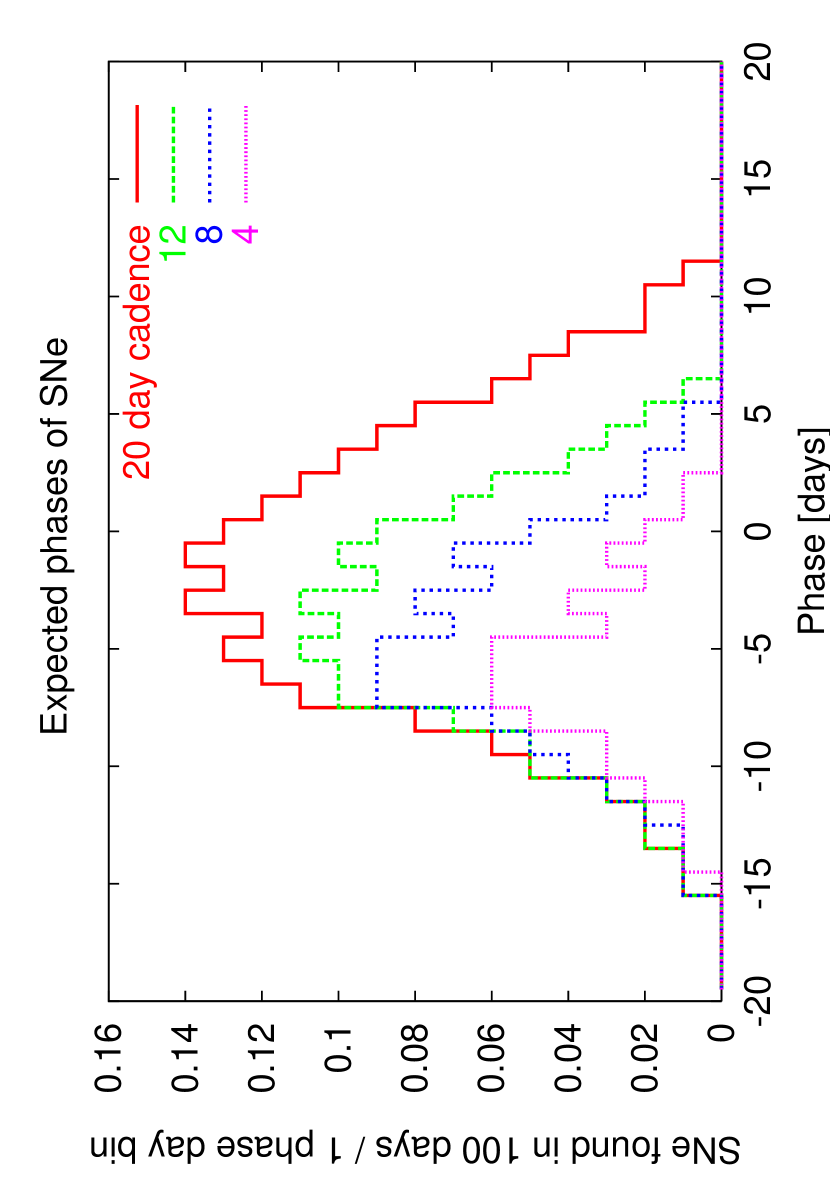
Figure 7: A simulation of the expected number of supernovae found at a given phase for different sky coverage cadences. Shorter sky coverage cadences result in fewer overall supernovae and the same number of early supernovae. See text (Sec. 7) for details of this simulation.

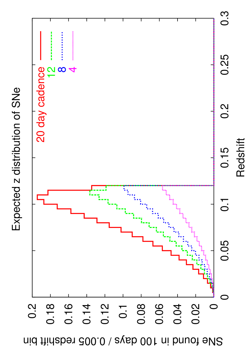
Figure 8: A simulation of the expected number of supernovae found at different redshifts for different sky coverage cadences. In reality, the sharp cutoff is smoothed out by the dispersion in SN Ia light curves. See text (Sec. 7) for details of this simulation.

The actual discovery phase of SNfactory SNe Ia with sufficient coverage to determine a good date of maximum is given in Fig. 9. These phases were determined from NEAT follow-up observations of the SNfactory SNe Ia by fitting the observed light curves with the same snminuit program used by the SCP to fit the time of maximum B-band brightness, maximum magnitude, and stretch of SNe Ia cosmological studies. Fig. 10 shows a comparison of Fig. 7 & 9. Note that the Poisson noise prevents a meaningful comparison of the observed and model distributions. Fig. 12 shows a comparison of the discovery phases expected from the simulation described in Sec. 9 with the known phases observed supernovae as described in Fig. 9.

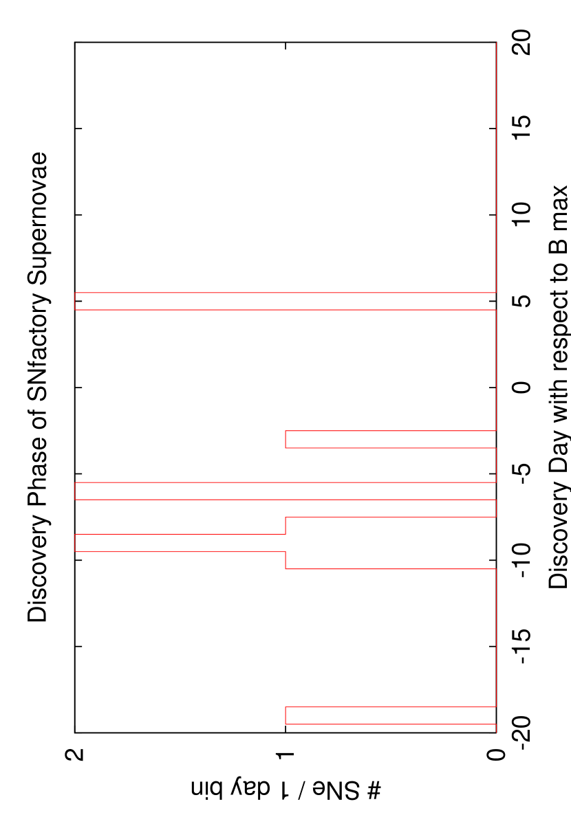
Figure 9: The distribution of discovery epochs for the SNe Ia found in the SNfactory data set with well-sampled lightcurves sufficient to determine the date of maximum light using the SCP light-curve fitting code snminuit.

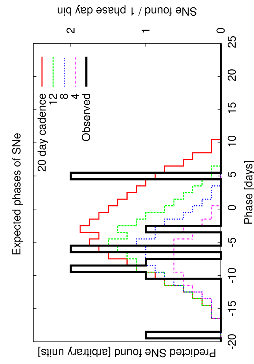
Figure 10: Fig. 7 compared with Fig. 9. The distribution of discovery epoch for the SNe Ia found in the SNfactory data set (heavy line) compared with the model described in Section 6.

Figure 11: The discovery epoch distribution for the Monte Carlo model described in Sec. 9.

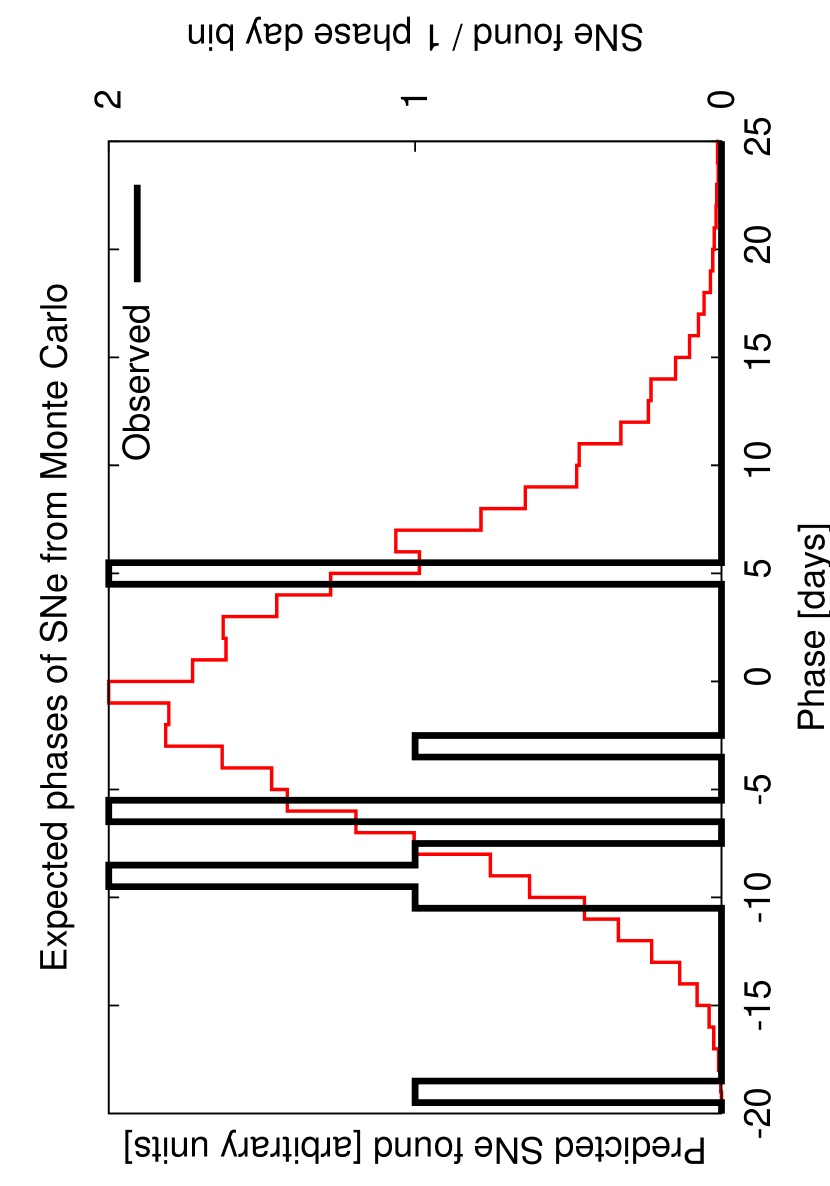
Figure 12: The discovery epoch distribution for the Monte Carlo model described in Sec. 9 and shown in Fig. 11 compared with the phases of the actual supernovae found shown in Fig. 9.

8 A Quick SN Ia Rate Calculation

This section presents a quick calculation of the SN Ia rate from a sub-sample of the SNfactory prototype search to illustrate the basic ingredients introduced in Eq. 2. The following section, Sec. 9, will present a more accurate and significantly more involved calculation of the SN Ia rate from a portion of the SNfactory prototype search.

In the month of March, 2003, there were $392.54\hbox{\hbox to0.0pt{$\sqcap$\hss}$\sqcup$}\hbox{${}^{\circ}$}$ worth of images subtracted to a limiting magnitude $<19.5$. There were 32 SNe found with a discovery magnitude $<19.5$ during this time. These subtractions were generally done against year-old reference images. Incorrectly taking a control time of 1 month for every square degree searched, one gets 32 SNe / $392.54\hbox{\hbox to0.0pt{$\sqcap$\hss}$\sqcup$}\hbox{${}^{\circ}$}$ / 1 month brighter than $19.5$ magnitude. Converting $19.5$ to a distance requires the use of the distance modulus,

$$\mu=m-M=5\log_{10}(r/[\mathrm{Mpc}])+25.$$ (4)

The distance, $r$, can then be expressed as

$$r=10^{(\mu-25)/5}~{}\mathrm{Mpc}.$$ (5)

Assuming a maximum SN Ia brightness of $-19.5$ magnitudes, or $\mu=19.5-(-19.5)=39.0$ , gives

$$r=10^{(39.0-25)/5}~{}\mathrm{Mpc}=631~{}\mathrm{Mpc}.$$ (6)

Integrating the solid angle of areal coverage gives a volume, $V$, of

$$V = \frac{\Omega}{3}r^{3},$$ (7)

where

$$\Omega = 4\pi\frac{392.54\hbox{\hbox to0.0pt{$\sqcap$\hss}$\sqcup$}\hbox{${}^{\circ}$}}{41,253\hbox{\hbox to0.0pt{$\sqcap$\hss}$\sqcup$}\hbox{${}^{\circ}$}}=0.1196,$$ (8)

and thus

$$V = \frac{0.1196}{3}(631~{}\mathrm{Mpc})^{3}.$$ (9)

Out of the $n_{\mathrm{total}}=65$ supernovae typed during the SNfactory prototype search phase, $n_{\mathrm{Ia}}=42$ were SNe Ia. Integrating over Eq. 2 by taking $(\frac{n_{\mathrm{Ia}}}{n_{\mathrm{total}}})~{}32\approx 20$ as the number of SNe Ia discovered in March, 2003, assuming a constant control time out to the limiting magnitude of $-19.5$, and neglecting the time-dilation factor, $1+z$, results in a SN Ia rate of

$$r_{V}=\frac{20~{}\mathrm{SN}}{(\frac{0.1196}{3})(631~{}\mathrm{Mpc})^{3}(1~{}\mathrm{month})}\frac{12~{}\mathrm{months}}{1~{}\mathrm{year}}=2.4\times 10^{-5}~{}\mathrm{SN}/\mathrm{Mpc}^{3}/\mathrm{year}$$ (10)

There are clearly many oversimplications in this calculation. First, there has been no accounting for repeated observations of the same field. Second, there has been no true calculation of control time. These factors will decrease the volume searched and thus increase the rate for the same number of supernova.

The next method will present a similar analysis to that above, but will take into account the repeated observations of the same fields during March 2003 as per the NEAT observing strategy. A one-month control time will still be assumed for each field. This areal accounting divides the sky up into equal area sections and increments the count of each section for every subtractions that overlaps that area by at least $50\%$. As part of a given subtraction may be masked, it will be difficult to calculate the exact overlap. To account for this masking, the contribution of each subtraction is normalized by ensuring that the amount of area added matches the area of the subtraction.

A more detailed analysis with areal tracking reveals there is little duplication of areal coverage in the previous calculation. Using bin sizes of $0.5$ degrees on a side, placing each subtraction in the appropriate bin, and adding up the areas of the subtractions in each bin to a maximum of the bin area ($0.25$ $\sqcap$$\sqcup$^∘) gives $347.51$ $\sqcap$$\sqcup$^∘ of unique area searched. The updated supernovae rate from this calculation is then

$$r_{V} = \frac{20~{}\mathrm{SN}}{\mathrm{month}}\left(\frac{4}{3}\pi\frac{347.51\hbox{\hbox to0.0pt{$\sqcap$\hss}$\sqcup$}\hbox{${}^{\circ}$}}{41,253\hbox{\hbox to0.0pt{$\sqcap$\hss}$\sqcup$}\hbox{${}^{\circ}$}}(631~{}\mathrm{Mpc})^{3}\right)^{-1}\frac{12~{}\mathrm{months}}{1~{}\mathrm{year}}$$ (11)

$$r_{V} = 2.84\times 10^{-5}~{}\mathrm{SN}/\mathrm{yr}/\mathrm{Mpc}^{3}$$ (12)

9 The Right Way: Control-Time Monte Carlo Simulation

To integrate the sampling of the control times and efficiency measurements, a database of simulated supernovae was created. Two hundred million SNe Ia were included in this database, covering the sky from $+50$ to $-50$ degrees in declination, at all RA values, and in the redshift range from $z=0$ to $z=0.4$, This sample was created with a constructed SNe Ia rate of 1 SN/Mpc³/century. Taking the literature SNe Ia rate (Cappellaro et al. 1999a; Pain et al. 2002) of roughly $1\times 10^{-4}$ SN/Mpc³/century, roughly 10,000 supernovae were simulated for each supernova expected from the search. The SNe Ia were created with dates of maximum B-band light spread over four years representing 2001–2004. The approach introduced in this section is dubbed the Control-Time Monte Carlo method because it departs from other methods in its proper temporal tracking of simulated supernovae in the control-time measurement. The explicit dates given to simulated supernovae allowed the supernovae found in different subtractions of the same area of sky to be tracked appropriately and not double-counted. The simulated SNe Ia were placed randomly over the sky with a neighbor-avoidance check to ensure a spacing of at least 10^′′ between simulated SNe. This strategy avoided object confusion in the subtractions performed with the simulated SNe Ia. The number of objects found scales as the number of objects in the sample while the number of coincident object rates scales as the square of the number of objects. Thus, the probabilities of observing coincident supernovae in the Universe are far smaller than in an unconstrained sample of 200 million objects across half of the sky.

The subtractions are rerun with the simulated supernovae added from this sample. Each supernova in the RA and Dec range of the subtraction was placed on the constituent reference and search images of the subtraction. The SN Ia flux is calculated based on the JD of each particular image and the redshift and stretch of the simulated supernova. For each image, a normalized PSF was constructed from the good stars on the image. This PSF was multiplied by the flux appropriate to the magnitude of the simulated object and added to the image. These images were then used in a new simulated subtraction based on the original subtraction to measure the efficiency of the original subtraction. The simulated subtraction used the original good star list from the original subtraction in the calculation of flux ratios, PSF widths, and other properties, just as was done in the original subtraction. These subtractions duplicated the steps and parameters used in the original subtraction.

For each a subtraction, a list of the fake candidates was saved to a file of the form $<$subtraction_name$>$.genfakes.nc in the DEEPIMAGEPATH. For this study, just SNe Ia were considered, but a future analysis should include different assumptions of core-collapse rates and magnitude dispersions in addition to the SN Ia rates.

To analyze the efficiency of each subtraction, a pair of IDL routines, analyzefakes.pro and analyzeallfakes.pro, were written along with some helper scripts, to calculate the number of SNe Ia expected for a given supernova rate. Any desired model of the SN rate as a function of redshift can be reconstructed from the simulated supernovae by appropriate re-weighting of the redshift distribution. The number of simulated SNe Ia recovered with a given model of the SN Ia rate as a function of redshift was compared with the number of SNe Ia actually found. The distribution of recovered simulated SNe Ia as a function of redshift and as a function of discovery magnitude is also compared with Fig. 3 and Fig. 2 to check consistency with the sample. For the histograms presented in this chapter with numbers of supernovae in a given magnitude or redshift bin, a relative error is calculated using Poisson statistics (for $n\mathrel{\hbox{\hbox to0.0pt{\hbox{\lower 4.0pt\hbox{$\sim$}}\hss}\hbox{$>$}}}5$, $n_{\sigma}\approx\sqrt{n}$). However, the actual comparisons of model and observation is to the overall number of supernovae found (i.e., this is an unbinned analysis). This total is itself governed by Poisson statistics as it is still a counting statistic of uncorrelated events. This total and associated uncertainty is then used when comparing the agreement of the simulated curves with the observed rates to determine if a given model is consistent with the SNfactory results.

1 Stretch Range

The stretch of a SN Ia affects its light curve and thus control time for a given search. To estimate the effect of SN Ia of different stretches on the calculated rate, the time evolution of the template supernovae was adjusted by $t^{\prime}=st$ and the peak V-magnitude was similarly changed by $M^{\prime}_{V}=M_{V}-\alpha(s-1)$, where $\alpha=1.18$ was taken from the value given for all SCP SNe Ia in Table 8, row 6, of Knop et al. (2003).

The impact of different stretch values can be seen in its effects on the control time and the limiting magnitude of the search. A dimmer, faster-rising and falling supernova has a reduced effective control time as the supernova is visible for less time. This effect scales with the stretch value and holds equally at any redshift. The visible time of the supernova is further reduced for a lower-stretch SN Ia as it is dimmer and thus below the limiting magnitude of a given search for more of its light curve. For the Control-Time Monte Carlo method described in Sec. 9, a Gaussian stretch distribution centered around 1 with a $\sigma=0.1$ was used to model the observed diversity in SN Ia light curves. Sec. 1 discusses the effect of assuming different stretch distribution models.

2 Modeling of the Host Galaxy Population

The percentage increase cut discussed in Sec. 5 highlights the need for a proper understanding of the host galaxy population observed in the SNfactory search. The Sloan Digital Sky Survey provides the most complete galaxy sample to date for estimating the galaxy population observed in the SNfactory search (Blanton et al. 2003a, b; Shen et al. 2003).

Assuming no evolution in galaxy properties out to a redshift of $z=0.2$, the SDSS DR1 galaxy sample can be scaled to model the host galaxy population of the SNfactory search. In the modeling of the effect of the underlying host galaxy on the detection of a supernova in the search, the immediately crucial parameters are the luminosity of the galaxy, the spatial luminosity distribution of the galaxy, the redshift of the galaxy and the effective seeing of the subtraction. The first two parameters are dependent on the galaxy population, obtainable from Shen et al. (2003); the redshift can be simulated assuming a constant galaxy population out to $z=0.2$; and the seeing of the subtraction, dependent on the observational conditions of the images that went into the subtraction, is recorded in the subng database table as part of the original subtraction.

Based on Strauss et al. (2002), Shen et al. (2003) estimate their sample to be complete for galaxies with apparent magnitudes between $r=15.0$ and $r=17.5$. Due to the nature of the SDSS survey, imaging and spectroscopic data are available for all galaxies that make up the complete Shen et al. (2003) sample. The fluxes of galaxies in the full redshift range of interest ($0.0<z<0.2$) can be reconstructed by scaling the radius used to measure aperture fluxes to the desired redshift. Ensuring full coverage in the search redshift range is complicated by the distribution of absolute magnitudes of the galaxies. For each absolute magnitude, there is a different maximum redshift at which it is observable above the $r>17.5$ cutoff. Assuming the galaxy luminosity function does not evolve out to $z=0.2$, a full sample can be constructed by weighting each supernova by the inverse of its covered volume as defined by the $z_{\mathrm{max}}$ at which it would be observable. This was the approach taken by Shen et al. (2003). A similar technique is used here to arrive at a complete sample of galaxies out to a given redshift from which to draw the supernovae. It is possible that the very faintest galaxies are not well accounted for by this analysis, but, assuming that supernovae are strongly correlated with luminosity, the potential absence of these galaxies should not significantly affect these results.

The galaxy stamps from the sample described by Shen et al. (2003) were retrieved from the SDSS archive server in the form of fpAtlas files. Image stamps and photometric calibration information were retrieved as part of an SQL query to the SDSS database. The galaxy stamp images were analyzed using the same fisofind code that is used in the standard SNfactory data reduction. The fisofind analysis gave the isophotal extent of the galaxy of pixels at least $3~{}\sigma$ above the sky noise background of the SDSS images.

For each simulated supernova, an amount of host-galaxy light appropriate for the effective seeing of the subtraction and the redshift of the supernova was drawn from a galaxy luminosity distribution function calculated from the Shen et al. (2003) sample. The redshift of the supernovae was included by calculating the appropriate surface brightness dimming and radial size decrease for a cosmological model with ${\Omega}_{M}$ $=0.3$, ${\Omega}_{\Lambda}$ $=0.7$. The search scores of each simulated supernova were re-calculated to include the effect of the host-galaxy light. To incorporate the galaxy flux background into the rate calculation, a grid of aperture bins was constructed to record the probability distribution of host-galaxy background light as a function of aperture and redshift. For each aperture bin, the flux for that aperture was calculated for each galaxy pixel found by fisofind. The results for all of the galaxies in the sample were combined to construct an aperture “brightness” distribution for all galaxy pixels.

Because of this approach, the SN rates can not be calculated as a function of volume without taking into consideration an assumed galaxy luminosity distribution. However, having to include a galaxy luminosity function also makes it clear that supernova searches are sensitive to the host galaxy population and thus an understanding of the true coverage of a given search is dependent on an understanding of the galaxy population underlying the supernovae.

3 Milky Way Extinction

Dust in our own galaxy results in reduced sensitivity along certain lines of sight. Unlike high-redshift searches, which specifically choose low-dust regions, the SNfactory search covers a large fraction of the sky and encompasses a wide range of Milky Way extinctions. The dust maps of Schlegel et al. (1998) were used to include this effect in the Control-Time Monte Carlo simulation.

The dust maps were downloaded to PDSF along with the companion IDL code to read the maps. A wrapper program was written to calculate the extinction for SNe Ia observed with the NEAT system response function as discussed in Appendix 10 (see Fig. 7). This program measures the effect of an $R_{V}=3.1$ extinction law (Cardelli et al. 1989) on the magnitudes of the simulated supernova. When placing simulated supernova on the NEAT images, a spectrum of a SN Ia at the appropriate phase (assuming stretch applies to spectral phase as well as photometric phase) was convolved with the NEAT system response. The difference between applying an $R_{V}=3.1$ extinction law,

$$A_{\lambda}=A_{V}/E(B-V)\times(0.574-(0.527/R_{V}))\times\lambda^{-1.61},$$ (14)

and assuming no extinction was integrated over the wavelength range of the NEAT detectors and converted to a $\Delta m$,

$$\Delta m=-2.5\log{\frac{\int_{3000\AA}^{10000\AA}{10^{-0.5\times A_{\lambda}}r_{\mathrm{NEAT}}f_{\lambda}d\lambda}}{\int_{3000\AA}^{10000\AA}r_{\mathrm{NEAT}}f_{\lambda}d\lambda}},$$ (15)

which was then taken as the extinction for that line of sight and SN spectrum. This extinction was applied to the simulated supernova magnitudes that were injected into the component images. Fig. 13 shows the distribution of E(B-V) values for the subtractions in the sample of the SNfactory survey considered here.

Figure 13: The E(B-V) values for the RA and Dec values of the reference systems for the simulated subtractions used in the rates analysis presented in this chapter. The linear-linear plot on the left illustrates that the majority of the fields have E(B-V) values of less than $0.1$. The linear-log plot on the right demonstrates the power-law nature of the dust distribution covered by this sample of the SNfactory survey.

As can be seen in Fig. 13, the $E(B-V)$ values for the NEAT fields searched ranged from a $0.005$–$0.6$. It is thus clearly important to include the modeling of the Milky Way extinction in a detailed calculation of the SN rates from this wide-field survey.

The contribution from host-galaxy dust extinction has been neglected here. This leads to an underestimate of the true supernova rate. The extinction due to host-galaxy dust is a general problem in supernova rate studies and there is no clear solution. However, as extinction is a line-of-sight effect, it would apply equally to galaxies at different redshifts if the evolution of host-galaxy dust with redshift were not significant. But, the dust content in galaxies does increase with redshift, as it should follow the increasing star formation rate, and a comparison of SN rates out to higher redshifts, $z>0.5$, will have to include modeling of host-galaxy dust extinction. For more discussion of the likely amount of host-galaxy extinction for different dust assumptions, see Commins (2004).

4 Efficiency as Measured by Control-Time Monte Carlo

The complete control-time measurement for the sample of the SNfactory prototype survey simulated to date is shown in Fig. 14 & 16. These figures show the “recovered” fraction of simulated supernovae—the simulated supernovae from the database that are detected as objects in the subtraction—and the “discovered” fraction—the fraction of simulated supernovae from the database that pass the default score cuts. The dotted curves shows the fraction of supernovae from the simulated supernova database that is recovered in the subtraction. The cutoff in the bright end is from detector saturation while the cutoff in the faint end is from signal-to-noise loss. The dashed curve underneath the dotted curve represents the number of recovered supernova that also pass the standard SNfactory cuts (see Sec. 9). While these cuts have evolved over time, all but two of the supernovae that have been found to date by the standard SNfactory search pipeline pass the current default cuts. The two exceptions are SNe that were discovered with NEIGHDIST scores $<0.5\hbox{${}^{\prime\prime}$}$; as a result, these SNe were excluded from this calculation of SN rates. The structure observed in Fig. 14 & 16 is a combination of the efficiencies of thousands of subtractions. The sensitivity variation between subtractions leads to the blurring of the edges of both the detection and recovery limits.

The efficiency of the SNfactory search as measured using the Control-Time Monte Carlo method is shown in Fig. 15 & 17. This figure shows the discovered fraction divided by the recovered fraction and is analogous to the standard treatment of efficiencies in other studies (e.g. Pain et al. (2002)), although those studies often include the areal loss from masked regions in their efficiency numbers as well.

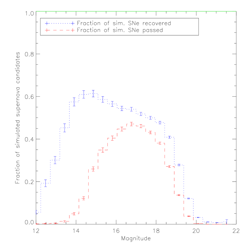
Figure 14: The recovered and discovered fraction of database supernova as a function of magnitude as measured using the analyzeallfakes.pro routine on the simulated subtractions run using the database of 200 million simulated SNe Ia. No correction for host galaxy light and the effect of the percent-increase cut has been applied here (see Fig. 16). The low fraction in the recovered discovered supernovae is mainly due to subtractions with short time baselines where the majority of the simulated supernovae were dimmer in the new images that in the reference images. See text (Sec. 4) for more details.

Figure 15: The fraction of simulated SNe Ia that pass the default score cuts as a function of magnitude as measured using the analyzeallfakes.pro routine on the simulated subtractions run using the database of 200 million simulated SNe Ia. No correction for host galaxy light and the effect of the percent increase score has been applied here (see Fig. 17). This plot is analogous to what most other analyses consider the efficiency of a search.

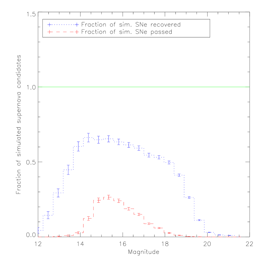
Figure 16: The recovered and discovered fraction of database supernova as a function of magnitude as measured using the analyzeallfakes.pro routine on the simulated subtractions run using the database of 200 million simulated SNe Ia. This plot includes the effect of host galaxy light in the reference and its effect on the percent increase score. The low fraction in the recovered discovered supernovae is mainly due to subtractions with short time baselines where the majority of the simulated supernovae were dimmer in the new images that in the reference images. See text (Sec. 4) for more details.

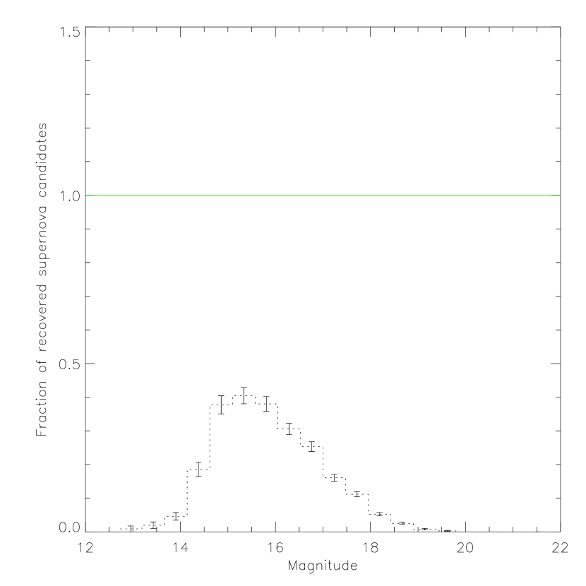
Figure 17: The fraction of simulated SNe Ia that pass the default score cuts as a function of magnitude as measured using the analyzeallfakes.pro routine on the simulated subtractions run using the database of 200 million simulated SNe Ia. The effect of the galaxy light as discussed in Sec. 5 is clear in comparison with Fig. 15. This plot is analogous to what most other analyses consider the efficiency of a search.

Fig. 14 & 15 are before including the effect of the host galaxy light through the percent increase threshold. Fig. 16 & 17 show the effect of the percent increase score in reducing the number of supernovae found.

While the cutoff at the fainter end for the passed candidates contrasted with the recovered candidates was not at all surprising, the bright-end cutoff was. This cutoff was due to an unexpected effect related to verifying that potential candidates were the same brightness in the constituent NEW images, properly weighted by the different errors. This score, SUB1MINSUB2, takes the difference in properly normalized aperture flux in SUB1 and SUB2 and divides by the quadrature sum of the errors. However, this score does not include the error in the calculation of the proper flux ratios to normalize the aperture flux values. The threshold that SUB1MINSUB2 must be less than $2.5$ quickly begins to be comparable to the zeropoint uncertainty at a magnitude of approximately $15$. The simulated supernovae exhibit this effect because of the uncertainty in the zeropoint used to calculate the appropriate fluxes for placing the simulated supernovae on the NEW images, while the actual sky objects suffer from this effect when the images are adjusted for this measured zeropoint difference. The simulated and real supernova suffer from this effect in the subtraction process and thus the effect on the simulated supernovae does appropriately track the effect on sky objects.

In addition to the obvious signal-to-noise threshold at the faint end of the sensitivity, the dispersion in the score used to discriminate against moving objects, DSUB1SUB2, becomes greater than the allowed thresholds due to positional uncertainties. Positional differences for the same object on different images can come from the transformation between the images, although normally images are matched to within a tenth of a pixel RMS, or, at the faint end, from variations in the position found as the center of the object due to noise fluctuations in the object. As the noise is proportional to the square root of the signal, these fluctuations are more pronounced for lower signal values. The simulated supernovae exhibit the same variation in DSUB1SUB2 because noise is added to each simulated supernova as it is placed on the individual images.

In general, this calculation of search efficiencies for the SNfactory has highlighted a number of quantitative scores that had a more significant effect on the search efficiencies than expected. An in-depth study of both real and simulated supernovae should be undertaken to adjust the scores and thresholds used to classify the objects found in the subtractions.

10 Systematic Uncertainties

A thorough understanding of biases and systematic errors is a key part of a proper calculation of SN rates. Possible sources of systematic uncertainty in this study include the diversity of SN Ia light curves, selection effects from the search efficiency and supernova type identification, the luminosity distribution of galaxies, host galaxy extinction, Milky Way extinction, magnitude calibration of the search fields, cosmological parameters, Malmquist bias, and the Shaw effect.

1 Diversity of SN Ia Light Curves

Light curves of SN Ia exhibit variation at the 30% level in both peak flux and rise and fall times (Goldhaber et al. 2001). This distribution has not been mapped out with sufficient sampling to determine the nature of SN Ia variation. For this analysis this variation was parameterized by the stretch value (Perlmutter et al. 1997; Goldhaber et al. 2001). The stretch of the SNe Ia was assumed to be normally distributed around a stretch value 1 with $\sigma=0.1$ (Perlmutter et al. 1998; Pain et al. 2002). For a further analysis, the simulated supernovae used in the rate calculation could be re-weighted to recreate any given model distribution of stretch values. For example, the difference between assuming a uniform distribution in stretch values from $0.9$ to $1.1$ and the normal distribution with $\sigma=0.1$ resulted in a $0.1\%$ difference in the SN Ia rate measured in this study. Taking twice this difference to represent the uncertainty in our current understanding of SN Ia diversity, the unknown variance of SN Ia light curves contributes $\pm 0.2\%$ to the systematic uncertainty in the rates presented here.

2 Luminosity Distribution of Galaxies

The underlying galaxy population enters the SN Ia rate per volume calculation through the modeling of the galaxy contribution in the reference image. Treatment of the galaxy luminosity distribution is discussed more thoroughly in Secs. 5 & 2. The dominant factor in the shifting of galaxies over the typical redshifts for this search, $z\sim 0.05$, is $1+z$ from the time dilation of the emission. This effect was included in the aperture measurements used as the basis underlying galaxy light modeling.

The conversion to SNu invokes the luminosity density of galaxies to convert from Mpc³ to $10^{10}$ L_⊙. Including an additional factor from the assumption that $g$-band galaxy magnitudes are equivalent $B$ galaxy magnitudes for the purposes of expressing galaxy brightness in solar luminosities, the conversion to SNu introduces an additional $\pm 5\%$ systematic uncertainty on the SN Ia rate in SNu, $r_{L}$.

3 Search Efficiency and Type Identification

The efficiency of the SNfactory search is well-understood and controlled using the Monte Carlo approach described in Sec. 9 and thus the uncertainty from the search efficiency is taken to be negligible. However, the type identification of the SNfactory prototype search requires a more detailed analysis to understand selection effects in supernova confirmation and spectral identification. As the SNfactory SNIFS instrument was not running during the prototype search and no spectroscopic follow-up was regularly available for the search, the spectral identification of these supernovae had to be provided by the community. This might lead to concerns that there was a selection bias in the supernovae that were spectroscopically confirmed. But, as discussed in Sec. 6, Fig. 4 demonstrates that there was no clear bias with respect to discovery magnitude for supernovae discovered brighter than $19.5$ magnitudes. In this analysis, only supernovae (both simulated and real) with discovery magnitudes brighter than 19.5 magnitudes were considered. As this calculation is for a constant supernova rate per physical volume as a function of redshift, selection effects of the type of the observed supernovae as a function of redshift are not important.

4 Magnitude Calibration

The magnitudes used for the simulated supernovae in this work were calibrated to the search images through a calibration to the USNO A1.0 catalog (Monet et al. 1996). This catalog has known systematic variations between POSS-E fields of $0.2$ magnitudes. However, the SNfactory search covered a large number of POSS-E fields ($>100$). Assuming that these variations are uncorrelated and centered around $0$, then this $\sim 20\%$ flux uncertainty is reduced to $20\%/\sqrt{100}=2\%$. Thus, one can roughly include the uncertainties in magnitude calibration as an additional source of systematic error on the measured rate at the $\pm 2\%$ level.

5 Cosmological Parameters

The value of the cosmological parameters $H_{0}$, ${\Omega}_{M}$ and ${\Omega}_{\Lambda}$ affect the calculation of distances and volume elements for this survey. While Freedman et al. (2001) measured $H_{0}=72\pm 8$ km/s/Mpc, the uncertainty in $H_{0}$ is factored out of the SN Ia rate in the $h^{3}$ term, for the SN Ia rate per Mpc³. In the expression of the SN Ia rate in terms of SNu there is one less apparent factor of $h$, but any interpretation of the result in terms of physical size effectively reinstates the factor of $h$. This leaves uncertainty in ${\Omega}_{M}$ and ${\Omega}_{\Lambda}$ as the dominant source of cosmological uncertainty in the numeric $r_{V}$ value found by this study. Recent studies of SNe Ia and the cosmic microwave background have provided constraints on these parameters to roughly $\pm 0.05$ (Knop et al. 2003; Spergel et al. 2003; Riess et al. 2004) and strongly indicate a flat Universe, ${\Omega}_{M}$ $+$${\Omega}_{\Lambda}$ $=1$ (ignoring curvature). While the variation in these parameters does not translate easily to the rate per either volume or luminosity, its effect can be estimated by considering the difference between the volume element at $z=0.1$ in an ${\Omega}_{M}$ $=0.25$, ${\Omega}_{\Lambda}$ $=0.75$ and an ${\Omega}_{M}$ $=0.35$, ${\Omega}_{\Lambda}$ $=0.65$ Universe. For this nearby search, the uncertainty in ${\Omega}_{M}$ and ${\Omega}_{\Lambda}$ contributes $\pm 2.4\%$ to the systematic uncertainty in either $r_{V}$ or $r_{L}$.

6 Extinction

As described in Sec. 3, the extinction from our own galaxy is modeled as part of the simulations using the dust maps of Schlegel et al. (1998). The extinction from the host galaxy was not modeled in the simulations. However, Commins (2004) used a combination of theoretical models and observational data to show that this effect does not evolve strongly with redshift, and so, in a comparison with supernova rates at different redshift, the effect of host galaxy extinction should not be corrected for (Pain et al. 2002). The absolute rate of supernovae as a function of underlying stellar population is of interest for other purposes, such as studies of chemical evolution of galaxies and initial mass and binary fractions of stellar populations. For these purposes careful attention should be paid to modeling the effect of host galaxy dust extinction to arrive at the “true” supernova rate.

7 Malmquist Bias

Malmquist bias (Malmquist 1924, 1936) is the simple recognition that in a magnitude-limited survey, there is a bias against finding dimmer objects at the limits of the survey. Put in the specific context of supernova, one will be biased toward finding fewer fainter supernovae at the limits of one’s redshift range. This effect is estimated here by doing a Monte Carlo study on the detection efficiency as a function of magnitude to determine the limiting redshift to which one has, in effect, conducted a volume-limited survey (Pain et al. 1996, 2002). For the SNfactory sample, this efficiency measurement is done on an image-by-image basis through the Control-Time Monte Carlo method, and only supernova that fall within the estimated volume sample are included. Thus, this technique automatically corrects for any Malmquist bias effect.

However, it should be noted that the SNe Ia generally are not sensitive to a strong Malmquist bias because their observed dispersion is low. Malmquist bias would be more of an issue for core-collapse supernovae.

8 The Shaw Effect

In 1979, Shaw wrote a short, succinct article that presented evidence for a significant bias against finding supernova near the centers of galaxies in photographic surveys (Shaw 1979). The basic issue was that the nucleus of many galaxies is saturated on a photographic plate. As a result, in this process, supernovae can not be detected within that region. However, the first-ever CCD search for supernovae (Muller et al. 1992) found no evidence for a Shaw effect.

Wang et al. (1997) conducted a study of “Supernovae and their Host Galaxies” and found that there were differences in the observed properties and types of supernova at varying projected radial distances from the center of the host galaxy. This distance is referred to as the projected galactocentric distance (PGD). Wang et al. (1997) confirmed the effect noted in Shaw (1979) and also found that there was a deficit of supernova at large PGD in nearby galaxies, possibly due to searches with fields of view smaller than some of the galaxies surveyed.

Fig. 18 shows a scatter plot of redshift versus PGD for the 70 SNfactory supernova with known redshifts (as of July 1, 2003). This plot shows no evidence of the Shaw effect. Compare with Fig. 1 of Shaw (1979) and note the absence of any region of avoidance in Fig. 18. The higher redshift regions are sparsely filled due to the limits of the search.

There is, however, a known bias in the PGD found as a function of redshift in the SNfactory search due to the finite angular resolution ability of the search telescopes. A $0.5$ pixel cutoff is used in the candidate screening on distance to the nearest object in the reference. This cutoff results in roughly a $0.5$” threshold (for the Palomar 48^′′ 3-CCD detector; for the MSSS 1.2-m, $0.67$”; and for the Palomar 48^′′ QUESTII, $0.44$”) that increases in physical distance with increasing redshift, as shown in Fig. 18.

In line with Wang et al. (1997), one could interpret Fig. 18 as also demonstrating a bias against finding supernova at large physical separation from the center of the apparent host in the nearby sample. However, the SNfactory/NEAT survey uses images on the order of $0.25\hbox{${}^{\circ}$}\times 0.25\hbox{${}^{\circ}$}$, so this deficit should not be a result of a limited field of view, as proposed by Wang et al. (1997) as an explanation for the effect in their study. We note that the SNfactory software masks out the entirety of any object with a sufficient number of saturated pixels to mask out bright stars that may contaminate large regions of the CCD. This same procedure will mask the entirety of a galaxy with a saturated region such as the core or a superimposed bright star. However, the number of galaxies at these low redshifts is very sparse and so there are fewer supernovae at those redshifts for a given solid angle covered.

Fig. 19 presents the same results as in Fig. 18 but in terms of projected arcseconds from the apparent host galaxy instead of projected physical distance. This representation makes it clear that the selection in terms of angular distance shows no clear trend as a function of $z$. With some allowance for fluctuation and statistical noise at any particular redshift, there is no clear deficit at any redshift.

Figure 18: The redshift versus projected galactocentric distance for a sample of 58 SNe with known redshifts found by the SNfactory search. No evidence for the Shaw effect is observed. The $0.5$” cutoff used by the SNfactory detection software is shown by the dashed line at the far left.

Figure 19: The redshift versus projected galactocentric angular separation for a sample of 58 SNe with known redshifts found by the SNfactory search. The $0.5$” cutoff used by the detection software due to seeing considerations is shown by the dashed line at the far left.

11 SN Ia Rate

A subsample of the subtractions from the SNfactory prototype search from September 2002 through May 2003 was used to generate a preliminary rate measurement using the technique described above. To avoid bias in the count of found supernovae, the simulated subtractions were run and debugged without reference to which nights or subtractions had real supernovae.

The simulated number of SNe Ia from the search was compared with the total effective number of SNe Ia found in the sample considered here. An analysis of the simulated subtractions found a predicted number of SNe Ia of

$$n_{\mathrm{Ia}}=5.67\pm 0.05\left[\frac{r_{V}}{1\times 10^{-4}~{}\mathrm{SNe~{}Ia}/\mathrm{yr}/\mathrm{Mpc}^{3}}\right],$$ (16)

where the uncertainty comes from the finite number of simulated supernovae used in the Control-Time Monte Carlo approach. As $n_{\mathrm{Ia}}=7.75$ SNe Ia were actually found in this sample, this preliminary study obtains a SN Ia rate of

$$r_{V}=3.67\ _{-1.66}^{+1.20}\mathrm{(stat)}\ _{-0.11}^{+0.11}\mathrm{(sys)}~{}h^{3}\times 10^{-4}~{}\mathrm{SNe~{}Ia/yr/Mpc}^{3},$$ (17)

where the listed uncertainties are statistical and systematic. While the statistical error bars remain significant in this analysis of a sample of the SNfactory prototype search, the strength of the Control-Time Monte Carlo approach is apparent in the small systematic uncertainties.

Conversion to SNu

To convert Mpc³ to SNu requires a measurement of the luminosity density of galaxies in the sample. The SDSS galaxy catalog provides the most thorough measurement of this density to date. Blanton et al. (2003a) found a luminosity density of $(1.78\pm 0.05)\times 10^{8}~{}h~{}L_{g\odot}/$Mpc³. Taking $L_{g\odot}\sim L_{B\odot}$, and inverting this luminosity density, one can convert from Mpc³ to $10^{10}~{}L_{B\odot}$,

$$\mathrm{SN~{}Ia~{}rate}~{}[\mathrm{SNu}]=\frac{56.2\pm 2.8}{h}\frac{\mathrm{Mpc}^{3}}{10^{10}L_{B\odot}}\mathrm{SN~{}Ia~{}rate}~{}[10^{-4}/\mathrm{yr}/\mathrm{Mpc}^{3}]$$ (18)

Thus the SN Ia rate can be expressed in SNu as

$$r_{L}=1.07\ _{-0.48}^{+0.35}\mathrm{(stat)}\ _{-0.03}^{+0.03}\mathrm{(sys)}~{}h^{2}~{}\mathrm{SNu}.$$ (19)

As shown Fig. 20, the SN Ia rate found here is consistent with the results of Muller et al. (1992), Cappellaro et al. (1999a), Hardin et al. (2000), Blanc (2002), and Pain et al. (2002). The statistical uncertainties on the current SNfactory rate measurement will be reduced with further analysis of the SNfactory prototype search. The current results from this and other nearby studies do not greatly constrain the SN Ia rate as a function of redshift. The improved constraints from a further analysis of the SNfactory search together with the intermediate-redshift ($z\sim 0.5$) SN Ia rate of Pain et al. (2002) will allow for an investigation of galaxy evolution and star formation rates over the past 5 billion years.

Figure 20: A comparison of the results of this preliminary study with previous SN Ia rate measurements: Muller et al. (1992), Cappellaro et al. (1999a), Hardin et al. (2000), Blanc (2002), and Pain et al. (2002). The statistical limits of this study will be improved with further work to be published in 2005. The results of each study have been standardized to $H_{0}=72$ km s^-1 Mpc^-1. The rate of Muller et al. (1992) has been assumed to be for $z=0.01$.

Part 3 The Hybrid Supernova 2002ic

Chapter 6 Photometry of SN 2002ic and Progenitor Mass-Loss

W. M. Wood-Vasey and L. Wang and G. Aldering

[The following was accepted for publication in ApJ, 2004.]

2004 May 6

1 Abstract

We present new pre-maximum and late-time optical photometry of the Type Ia/IIn supernova 2002ic. These observations are combined with the published V-band magnitudes of Hamuy et al. (2003) and the VLT spectrophotometry of Wang et al. (2004) to construct the most extensive light curve to date of this unusual supernova. The observed flux at late time is significantly higher relative to the flux at maximum than that of any other observed Type Ia supernova and continues to fade very slowly a year after explosion. Our analysis of the light curve suggests that a non-Type Ia supernova component becomes prominent $\sim 20$ days after explosion. Modeling of the non-Type Ia supernova component as heating from the shock interaction of the supernova ejecta with pre-existing circumstellar material suggests the presence of a $\sim 1.7\times 10^{15}$ cm gap or trough between the progenitor system and the surrounding circumstellar material. This gap could be due to significantly lower mass-loss $\sim 15~{}(\frac{v_{w}}{10~{}\mathrm{km/s}})^{-1}$ years prior to explosion or evacuation of the circumstellar material by a low-density fast wind. The latter is consistent with observed properties of proto-planetary nebulae and with models of white-dwarf + asymptotic giant branch star progenitor systems with the asymptotic giant branch star in the proto-planetary nebula phase.

2 Introduction

Historically, the fundamental division of supernova (SN) types was defined by the absence (Type I) or presence (Type II) of hydrogen in the observed spectrum. Later refinements distinguished Type Ia supernovae from other types of supernovae by the presence of strong silicon absorption features in their spectra (Wheeler & Harkness 1990; Filippenko 1997). Type Ia supernovae (SNe Ia) are generally accepted to result from the thermonuclear burning of a white dwarf in a binary system, whereas all the other types of supernovae are believed to be produced by the collapse of the stellar core, an event which leads to the formation of a neutron star or black hole.

While interaction with circumstellar material (CSM) has been observed for many core-collapse supernovae, the search for evidence of CSM around Type Ia SNe has so far been unsuccessful. Cumming et al. (1996) reported high resolution spectra of SN 1994D and found an upper limit for the pre-explosion mass-loss rate of $\dot{M}\sim 1.5\times 10^{-5}~{}M_{\odot}~{}\mathrm{yr}^{-1}$ for an assumed wind speed of $v_{w}=10$ km s^-1. However, they also note that this limit allows most of the expected range of mass-loss rates from symbiotic systems ($\frac{\dot{M}}{v_{10}}\mathrel{\hbox{\hbox to0.0pt{\hbox{\lower 4.0pt\hbox{$\sim$}}\hss}\hbox{$<$}}}2\times 10^{-5}~{}M_{\odot}$ yr^-1). On the other hand, the surprisingly strong high-velocity Ca II absorption and associated high degree of linear polarization observed in SN 2001el by Wang et al. (2003a) and the high velocity features in SN 2003du by Gerardy et al. (2004) have led these authors to suggest that the high velocity Ca feature could be the result of the interaction between the supernova ejecta and a CSM disk. About 0.01 M_⊙ of material is required in the disk, and the spatial extent of the disk must be small to be consistent with the absence of narrow emission lines at around optical maximum (Cumming et al. 1996). Due to the strength of the Ca II feature in SN 2001el, Wang et al. (2003a) speculated that the disk of SN 2001el may have been over-abundant in Ca II. In contrast, Gerardy et al. (2004) found that a standard solar abundance of Ca II is sufficient to explain the observed feature in SN 2003du (Gerardy et al. 2004), for which the high-velocity Ca II feature is significantly weaker than in SN 2001el.

Supernova 2002ic (Wood-Vasey 2002) is a very interesting event that shows both silicon absorption (Hamuy et al. 2002) and hydrogen emission (Hamuy et al. 2003). This SN is the first case for which there is unambiguous evidence of the existence of circumstellar matter around a SN Ia and is therefore of great importance to the understanding of the progenitor systems and explosion mechanisms of SNe Ia (Livio & Riess 2003). By studying the spectral polarimetry and the light curve of the H$\alpha$ line, Wang et al. (2004) found the spatial extent of the hydrogen-rich material to be as large as 10¹⁷ cm and distributed in a quite asymmetric configuration, most likely in the form of a flattened disk. The implied total mass of the hydrogen-rich CSM is a few solar masses. Similar conclusions were reached by Deng et al. (2004).

In this paper, we present new photometry of SN 2002ic and discuss the implications for the interaction of the ejecta and the CSM. Sec. 3 presents our data processing procedure and calibration for our photometry of SN 2002ic. In Sec. 4, we discuss the light curve of SN 2002ic and the immediate implications from our data. A more in-depth investigation and qualitative modeling of the light curve of SN 2002ic as an interaction of a SN Ia with surrounding CSM is presented in Sec. 6. Our discussion in Sec. 7 presents our interpretations of the structure of the CSM surrounding SN 2002ic. Finally, in Sec. 8 we present some intriguing possibilities for the progenitor system of SN 2002ic and speculate on other possible SN 2002ic-like events.

3 Data Processing for SN 2002ic

1 Data processing and Discovery

We discovered SN 2002ic on images from the NEAT team (Pravdo et al. 1999) taken on the Samuel Oschin 1.2-m telescope on Mt. Palomar, California. In preparation for searching, the images were transmitted from the telescope to the High-Performance Storage System (HPSS) at the National Energy Research and Scientific Computer Center (NERSC) in Oakland, California via the HPWREN (Braun 2003) and ESnet (U.S. Department of Energy 2004) networks. These data were then automatically processed and reduced on the NERSC Parallel Distributed System Facility (PDSF) using software written at Lawrence Berkeley National Laboratory by WMWV and the Supernova Cosmology Project.

The first-level processing of the NEAT images involved decompression and conversion from the NEAT internal format used for transfer to the standard astronomical FITS format, subtraction of the dark current for these thermoelectrically cooled CCDs, and flat-fielding with sky flats constructed from a sample of the images from the same night. These processed images were then loaded into an image database, and archival copies were stored on HPSS. The images were further processed to remove the sky background. An object-finding algorithm was used to locate and classify the stars and galaxies in the fields. The stars were then matched and calibrated against the USNO A1.0 POSS-E catalog (Monet et al. 1996) to derive a magnitude zeropoint for each image. There were typically a few hundred USNO A1.0 stars in each 0.25 $\sqcap$$\sqcup$^∘ image.

The supernova was discovered by subtracting PSF-matched historical NEAT images from new images, then automatically detecting residual sources for subsequent human inspection (see Wood-Vasey et al. (2004a)).

2 Photometry

For analysis, we assembled all NEAT images, including later images kindly taken at our request by the NEAT team.

Light curves were generated using aperture photometry scaled to the effective seeing of each image. A set of the 4 best-seeing ($<3$^′′) reference images was selected from among all NEAT Palomar pre-explosion images from 2001 of SN 2002ic. Multiple reference images were chosen to better constrain any underlying galaxy flux. The differential flux in an aperture around SN 2002ic was measured between each reference image and every other image of SN 2002ic. Aperture correction was performed to account for the different seeing and pixel scales of the images. The overall flux ratio between each reference image and light-curve image was tracked and normalized with respect to a primary reference image. This primary reference image was chosen from the reference images used for the image subtraction on which SN 2002ic was originally discovered. The flux differences calculated relative to each reference were combined in a noise-weighted average for each image to yield an average flux for the image. As the observations were taken within a span of less than one hour on each night, the results from the images of a given night were averaged to produce a single light curve point for that night.

The reference zeropoint calculated for the primary reference image from the above USNO A1.0 POSS-E calibration was used to set the magnitudes for the rest of the measured fluxes. Table 1 reports these magnitudes and associated measurement uncertainties. An overall systematic uncertainty in the zeropoint calibration is not included in the listed errors. The USNO A1.0 POSS-E catalog suffers from systematic field-to-field errors of $\sim 0.25$ magnitudes in the northern hemisphere (Monet et al. 1996). The conversion of POSS-E magnitudes to V-band magnitudes for a SN Ia is relatively robust, as a SN Ia near maximum resembles a $\sim 10,000$ K blackbody quite similar to Vega in the wavelength range from $4,500$–$10,000$ Å. At late times, the observations of Wang et al. (2004) show that the smoothed spectrum of SN 2002ic tracks that of Vega red-ward of 5,000 Å. We estimate that, taken together, the calibration of our unfiltered observations with these POSS-E magnitudes and the subsequent comparison with V-band magnitudes are susceptible to a $0.4$ magnitude systematic uncertainty. Any such systematic effect is constant for all data points and stems directly from the magnitude calibration of the primary reference.

However, the observed NEAT POSS-E magnitudes show agreement with the V-band magnitudes of Hamuy et al. (2003) and the V-band magnitudes obtained from integrating the spectrophotometry of Wang et al. (2004) to significantly better than any $0.4$ magnitude systematic uncertainty estimate. This synthesized VLT photometry is presented in Table 2. Comparing the photometry of SN 2002ic and nearby reference star with a similar color ($B-R=0.3$), we find agreement between the VLT V-band acquisition camera images and the NEAT images to within $\pm 0.05$ magnitudes. Given this good agreement, it appears that our POSS-E-calibrated magnitudes for SN 2002ic can be used effectively as V-band photometry points.

Mario Hamuy was kind enough to share his BVI secondary standard stars from the field of SN 2002ic. We attempted to use these stars to calculate the color correction from our POSS-E magnitudes to V-band, but our analysis predicted an adjustment of up to $+0.4$ magnitudes. This was inconsistent with the good agreement with the VLT magnitudes (calculated correction = $+0.1$ mag) at late times and with the Hamuy V-band points after maximum ($+0.4$ mag). This disagreement is not fully understood. We note, however, that the colors of the secondary standard stars did not extend far enough to the blue to cover the majority of the color range of the supernova during our observations (a common problem when observing hot objects such as supernovae). In addition, as there is no color information from before maximum light, it is possible that SN 2002ic does not follow the color evolution of a typical SN Ia.

Our newly reported pre-maximum photometry points (see Table 1 and Fig. 1) are invaluable for disentangling the SN and CSM components, which we now proceed to do.

4 Light Curve of SN 2002ic

The light curve of SN 2002ic is noticeably different from that of a normal SN Ia, as can be seen in Fig. 2, and as was first noted by Hamuy et al. (2003). The detection of hydrogen emission lines in the spectra of SN 2002ic in combination with the slow decay of the light curve is seen as evidence for interaction of the SN ejecta and radiation with a hydrogen-rich CSM (Hamuy et al. 2003; Wang et al. 2004). The profile of the hydrogen emission line and the flat light curves can be understood in the context of Type IIn supernovae as discussed in Chugai et al. (2002), Chugai & Yungelson (2004), and references therein.

The data presented here show that the slow decay has continued $\sim 320$ days after maximum at a rate of $\sim 0.004$ mag/day, a rate that is significantly slower than the $0.01$ mag/day decay rate expected from Co⁵⁶ decay (also see Deng et al. (2004)). In addition, our early-time points show that the light curve of SN 2002ic was consistent with a pure SN Ia early in its evolution. This implies that there was a significant time delay between the explosion and development of substantial radiation from the CSM interaction, possibly due to a a physical gap between the progenitor explosion and the beginning of the CSM. After maximum, we note the existence of a second bump in the light curve, which is put in clear relief by our photometry data on JD $2452628.6$. We interpret this second bump as evidence for further structure in the CSM.

5 Decomposition of SN Ia and CSM components

Hamuy et al. (2003) performed a spectroscopic decomposition of the underlying supernova and ejecta-CSM interaction components. We perform here an analogous photometric decomposition. To decompose the observed light curve into the contributions from the SN material and the shock-heated CSM, we first consider a range of light curve stretch values (Perlmutter et al. 1997), using the magnitude-stretch relation, $\Delta m=1.18~{}(1-s)$ (Knop et al. 2003), applied to the normal SN Ia template light curve of Goldhaber et al. (2001); we consider the remaining flux as being due to the SN eject-CSM interaction (see Fig. 2). At early times, the inferred contribution of the CSM is dependent on the stretch of the template chosen, but at later times the CSM component completely dominates for any value of the stretch parameter. It is not possible to disentangle the contribution of the CSM from that of the SN at maximum light, although a normal SN Ia at the redshift of SN 2002ic, $z=0.0666$ (Hamuy et al. 2003), corresponding to a distance modulus of $37.44$ for an $H_{0}=72$ km/s/Mpc (Freedman et al. 2001), would only generate about half of the flux observed for SN 2002ic at maximum. Hamuy et al. (2003) find that SN 2002ic resembles SN 1991T spectroscopically and note that SN 1991T/SN 1999aa-like events are brighter a month after maximum light than explainable by the standard stretch relation. A SN 1991T-like event (stretch$=1.126$, $\Delta m=0.15$, based on the template used in Knop et al. (2003) (A.J. Conley 2004, private communication)), would lie near the stretch$=1$ line of Fig. 2. The light curve of SN 2002ic for the first 50 days is thus much too luminous to be due entirely to a 91T-like supernova. In addition, the spectroscopically-inferred CSM-interaction contribution of Hamuy et al. (2003) (open triangles in Fig. 2) limits the SN contribution at maximum to that expected from a normal SN Ia. After 50 days, SN 2002ic exhibits even more significant non-SN Ia-like behavior.

We next use the formalism of Chevalier & Fransson (1994) to fit a simple interacting SN ejecta-CSM model to the observed data. While Chevalier & Fransson (1994) focus on SNe II, their formalism is generally applicable to SNe ejecta interacting with a surrounding CSM. We simultaneously fit the SN Ia flux and the luminosity from the SN ejecta-CSM interaction. Our analysis allows us to infer the integrated radial density distribution of the CSM surrounding SN 2002ic.

6 Simple Scaling of the SN Ejecta-CSM Interaction

Following the hydrodynamic models of Chevalier & Fransson (1994), we assume a power-law supernova ejecta density of

$$\rho_{\mathrm{SN}}\propto t^{n-3}r^{-n}$$ (1)

where $t$ is the time since explosion, $r$ is the radius of the ejecta, and $n$ is the power-law index of a radial fall-off in the ejecta density. Chevalier & Fransson (2001) note that for SNe Ia an exponential ejecta profile is perhaps preferred. However, this profile does not yield an analytical solution and so, for the moment, we proceed assuming a power-law profile. In Sec. 7 we explore the ramifications of an exponential ejecta profile.

Chevalier & Fransson (1994) give the time evolution of the shock-front radius, $R_{s}$, as

$$R_{s}=\left[\frac{2}{(n-3)(n-4)}\frac{4\pi v_{w}}{\dot{M}}A\right]^{1/(n-2)}t^{(n-3)/(n-2)},$$ (2)

where $v_{w}$ is the velocity of the pre-explosion stellar wind, $\dot{M}$ is the pre-explosion mass-loss rate, and $A$ is a constant in the appropriate units for the given power-law index $n$.

Taking the parameters in the square brackets as fixed constants, we can calculate the shock velocity, $v_{s}$, as

$$v_{s}=\left[\frac{2}{(n-3)(n-4)}\frac{4\pi v_{w}}{\dot{M}}A\right]^{1/(n-2)}\left(\frac{n-3}{n-2}\right)t^{-1/(n-2)}.$$ (3)

Thus the shock velocity goes as

$$v_{s}\propto t^{-\alpha},$$ (4)

where

$$\alpha=\frac{1}{n-2}.$$ (5)

We assume that the luminosity of the ejecta-CSM interaction is fed by the energy imparted at the shock front and view the unshocked wind as crossing the shock front with a velocity of $v_{s}+v_{w}\approx v_{s}$. As the wind particles cross the shock front, they are thermalized and their crossing kinetic energy, $\mathrm{K.E.}=\mbox{$\frac{1}{2}$}\rho_{w}v_{s}^{2}dV$, is converted to thermal energy. Putting this in terms of the mass-loss rate, $\dot{M}$, we can express the CSM density as

$$\rho_{w}=\frac{\dot{M}}{4\pi R_{s}^{2}v_{w}},$$ (6)

and we can calculate the energy available to be converted to luminosity, $L$, as

$$L=\alpha(\lambda,t)\frac{d}{dt}\mathrm{K.E.}=\alpha(\lambda,t)\frac{1}{2}\frac{\dot{M}}{4\pi R_{s}^{2}v_{w}}v_{s}^{2}dV=\alpha(\lambda,t)\frac{1}{2}\frac{\dot{M}}{4\pi R_{s}^{2}v_{w}}v_{s}^{2}v_{s}4\pi R_{s}^{2}.$$ (7)

The luminosity dependence on $R_{s}$ drops out and we have

$$L=\alpha(\lambda,t)\frac{d}{dt}\mathrm{K.E.}=\alpha(\lambda,t)\frac{1}{2}\frac{\dot{M}}{v_{w}}v_{s}^{3}.$$ (8)

A key missing ingredient is a more detailed modeling of the kinetic energy to optical luminosity conversion term, $\alpha(\lambda,t)$. We note that the available kinetic energy is on the order of $1.6\times 10^{44}$ erg s^-1 for $\dot{M}=10^{-5}~{}M_{\odot}$ yr^-1, $v_{s}=10^{4}$ km s^-1, and $v_{w}=10$ km s^-1. This implies a conversion efficiency from shock interaction K.E. to luminosity of 50%, given the luminosity, $1.6\times 10^{44}$ erg s^-1, of SN 2002ic and the typical luminosity of a SN Ia near maximum of $0.8\times 10^{44}$ erg s^-1. Assuming this constant conversion produces reasonable agreement with the data, so we proceed with this simple assumption. Using Eq. 4 to give the time dependence of $v_{s}$, we obtain the time dependence of the luminosity,

$$L\propto v_{s}^{3}\propto t^{-3\alpha},$$ (9)

which can be expressed in magnitude units as

$$m_{\mathrm{ejecta-CSM}}=C-\frac{5}{2}\log_{10}{t^{-3\alpha}}=C+\frac{15}{2}\alpha\log_{10}{t},$$ (10)

where $C$ is a constant that incorporates $\dot{M}$, $\rho_{\mathrm{SN}}$, $v_{w}$, $n$, and the appropriate units for those parameters. The difference in magnitude between two times, $t_{1}$ and $t_{2}$, then becomes

$$m_{t_{2}}-m_{t_{1}}=\frac{15}{2}\alpha\log_{10}{\frac{t_{2}}{t_{1}}}.$$ (11)

We obtain a date of B-maximum for the supernova component of $2452606$ JD from our SN Ia-light curve analysis. Our fit yields an $\alpha=0.16\Rightarrow n=8.5$ for any fixed $\dot{M}$ and $v_{w}$. This $n$ is squarely in the range of values suggested by Chevalier & Fransson (1994) as being typical for SN ejecta. While Chevalier & Fransson (1994) is framed in the context of SNe II, their formalism applies to any SN explosion into a surrounding medium whose ejecta density profile is described by their analytic model.

The interaction scaling relations presented above are useful for decomposing the interaction and supernova contributions to the total light curve of SN 2002ic. This simple, analytic description approximates our data reasonably well. However, more sophisticated theoretical calculations, which are beyond the scope of this paper, are necessary to more quantitatively derive the detailed physical parameters of the SN ejecta and the CSM (see Chugai & Yungelson (2004)).

7 Discussion

1 Inferred CSM structure and Progenitor Mass-Loss History

We can match the inferred SN ejecta-CSM component of Hamuy et al. (2003) with the interaction model described above and reproduce the light curve near maximum light by adding the flux from a normal SN Ia. Fig. 3 shows our model fit in comparison with the observed light curve of SN 2002ic. Note that our model does not match the observed bump at 40 days after maximum.

Hamuy et al. (2003) note a similar disagreement, but the data we present here show that this region is clearly a second bump rather than just a very slow decline. This discrepancy could be explained by a change in the density of the circumstellar medium due to a change in the progenitor mass-loss evolution at that point. In fact, our simple fit is too bright before the bump and too dim during the bump, implying more structure in the underlying CSM than accounted for in our model. Any clumpiness in the progenitor wind would have to be on the largest angular scale to create such a bump and would not explain the new decline rate shown by our observations to extend out to late time . We find that our data are consistent with a model comprising three CSM density regions: (i) an evacuated region out to $20v_{s}$ days; (ii) CSM material at a nominal density ($\rho\propto r^{-2}$) out to $\sim 100v_{s}$ days; and (iii) an increase in CSM density at $\sim 100v_{s}$ days, with a subsequent $r^{-2}$ fall-off extending through the $800v_{s}$ days covered by our observations. This model agrees well with the light curve of SN 2002ic, but, as it involves too many parameters to result in a unique fit using only the photometric data, we do not show it here.

Our data, particularly the pre-maximum observations, provide key constraints on the nature of the progenitor system of SN 2002ic. In the context of our model, a mass-loss gradient of some form is required by our early data points. As a computational convenience, our model assumes that the transition to a nominal circumstellar density is described by $\sin(\frac{t}{20~{}\mathrm{days}})$. If the mass-loss rate had been constant until just prior to the explosion, then the $t^{-3\alpha}$ model light curve would continue to curve upward and significantly violate our first data point at the $7\sigma$ level (as shown by the line extended from the ejecta-CSM component in Fig. 3). If the conversion of kinetic energy to luminosity is immediate and roughly constant in time, as assumed in our model, we would conclude that a low-density region must have existed between the star and $20$ days$\cdot v_{s}$ out from the star. For example, as a stellar system transitions from an AGB star to a proto-planetary nebula (PPN), it changes from emitting a denser, cooler wind, to a hotter, less dense wind (Kwok 1993). This hot wind pushes the older wind out farther and creates a sharp density gradient and possible clumping near the interface between the cool and hot winds (Young et al. 1992). This overall structure is similar to that which we infer from our modeling of SN 2002ic. Assuming a SN ejecta speed of $v_{s}=30,000$ km s^-1 and a progenitor star hot wind speed of $v_{w}=100$ km s^-1 (Young et al. 1992; Herpin et al. 2002), we conclude that the hot wind must have begun just $\sim 15$ years prior to the SN explosion. Alternatively, there is also the possibility that the conversion from kinetic energy to optical luminosity is for some reason significantly less efficient at very early times.

It is interesting to note that the observed light curve decline rate of SN 2002ic after $40$ days past maximum light is apparently constant during these observations. Spectroscopic study (Wang et al. 2004) shows the highest observed velocity of the ejecta to be around $11000$ km s^-1 at day $200$ after maximum light. If we assume a constant expansion rate, these observations of continuing emission through $\sim 320$ days after maximum provide a lower limit of $\sim 3\times 10^{16}$ cm for the spatial extent of the CSM. Compared to a nominal pre-explosion stellar wind speed of $10$ km s^-1, the ejecta is moving $\sim 1000$ times more rapidly and thus has overtaken the progenitor wind from the past $\sim 800$ years. The overall smoothness of the late-time light curve shows the radial density profile of the CSM to be similarly smooth and thus implies a fairly uniform mass-loss rate between $100$–$800$ years prior to the SN explosion.

We take the lack of enhanced flux at early times and the bump after maximum light as evidence for a gap between the SN progenitor and the dense CSM as well as a significant further change in the mass-loss of the progenitor system $\sim 100$ years prior to the SN explosion.

2 Reinterpretation of Past SNe IIn

These new results prompt a reexamination of supernovae previously classified as Type IIn, specifically SN 1988Z (Pollas et al. 1988; Stathakis & Sadler 1991), SN 1997cy (Sabine et al. 1997; Turatto et al. 2000; Germany et al. 2000), and SN 1999E (Cappellaro et al. 1999b; Siloti et al. 2000; Rigon et al. 2003). These supernovae bear striking similarities in their light curves and their late-time spectra to SN 2002ic. However, SN 2002ic is the only one of these supernovae to have been observed early in its evolution. If SN 2002ic had been observed at the later times typical of the observations of these Type IIn SNe, it would not have been identified as a Type Ia. It is interesting to note that Chugai & Danziger (1994) found from models of light curves of SN 1988Z that the mass of the SN 1988Z supernova ejecta is on the order of 1 $M_{\odot}$, which is consistent with a SN Ia.

We next explore the possibility that SN 1997cy and SN 1999E (a close parallel to SN 1997cy) may have been systems like SN 2002ic. Hamuy et al. (2003) found that available spectra of SN 1997cy were very similar to post-maximum spectra of SN 2002ic. We complement this spectroscopic similarity with a comparison of the photometric behavior of SN 1997cy and SN 2002ic. As shown in Fig. 4, the late-time behavior of both SNe appear remarkably similar with both SNe fading by $\sim 2.5$ magnitudes 8 months after their respective discoveries. The luminosity decay rate of the ejecta-CSM interaction is directly related to the assumed functional form for the ejecta density and the mass-loss rate (Eq. 1). The observed late-time light curves of SN 1997cy and SN 1999E clearly follow a linear magnitude decay with time, which implies an exponential flux vs. time dependence: $m\propto t\Rightarrow\mathrm{flux}\propto e^{Ct}$. If the ejecta density followed an exponential rather than a power-law decay, the magnitude would similarly follow a linear magnitude-time decay. Fig. 5 shows a fit to the light curve of SN 2002ic using the framework of Sec. 6 but using an exponential SN-ejecta density profile. Chevalier & Fransson (2001) suggest that SNe Ia follow exponential ejecta profiles (Dwarkadas & Chevalier 1998) while core-collapse SNe follow power-law decays (Chevalier & Soker 1989; Matzner & McKee 1999). Thus, if SN 1997cy and SN 1999E had been core-collapse events, they would have been expected to show power-law declines. Instead, their decline behavior lends further credence to the idea that they were SN Ia events rather than core-collapse SNe. Although we modeled the light curve of SN 2002ic using a power-law ejecta profile, SN 2002ic was not observed between 100 and 200 days after explosion, so its decay behavior during that time is not well constrained. Its late-time light curve is consistent with the linear magnitude behavior of SN 1997cy. We fit such a profile to our data (see Fig. 5 & 6) and arrive at an exponential fit to the flux of the form $e^{-0.003t}$ where $t$ is measured in days. As the solution for the SN-ejecta interaction is not analytic, we cannot immediately relate the exponential decay parameter to any particular property of the SN ejecta. Taken together in the context of the Chevalier & Fransson (1994) model, SN 2002ic, SN 1997cy, and SN 1999E lend support to numerical simulations of the density profiles of SNe Ia explosions.

If we take the time of maximum for SN 1997cy to be the earliest light curve point from Germany et al. (2000) and shift the magnitudes from the redshift of SN 1997cy, $z=0.063$ (Germany et al. 2000), to the redshift of SN 2002ic ($z=0.0666$), we find that the luminosity of both SNe agree remarkably well. This further supports that hypothesis that SN 1997cy and SN 2002ic are related events. However, we note that the explosion date of SN 1997cy is uncertain and may have been 2–3 months prior to the discovery date (Germany et al. 2000; Turatto et al. 2000).

Fig. 3 & 5 show that neither a power-law nor an exponential model allow for a significant ejecta-CSM contribution before maximum light. In each figure, the “[exp] ejecta-CSM fit w/o gap” line shows how the SN ejecta-CSM interaction would continue if the density profile remained the same. Both lines significantly disagree with the earliest light curve point. This is consistent with our earlier conclusion that the light curve is dominated by the SN until near maximum light.

3 Relation to Proto-Planetary Nebulae?

The massive CSM and spatial extent inferred for SN 2002ic are surprisingly similar to certain PPNe and the atmospheres of very late red giant stars evolving to PPNe. Such structures are normally short-lived (less than or on the order of $1000$ years). The polarization seen by Wang et al. (2004) suggests the presence of a disk-like structure surrounding SN 2002ic. Furthermore, the H$\alpha$ luminosity and mass and size estimates suggest a clumpy medium. Combined with the evidence presented here for a possible transition region between a slow and fast wind, we are left with an object very similar to observed PPNe. We encourage more detailed radiative hydrodynamic modeling of SNe Ia in a surrounding medium as our data provide valuable constraints on this important early-time phase.

Of particular interest are bi-polar PPNe where a WD companion emits a fast wind that shapes the AGB star wind while simultaneously accreting (Soker & Rappaport 2000) mass from the AGB star.

Typical thermonuclear supernovae are believed to have accretion time scales of $10^{7}$ years, yet several SNe Ia (SN 2002ic and possibly SN 1988Z, SN 1997cy, and SN 1999E) out of several hundred have been observed to show evidence for significant CSM. If the presence of a detectable CSM is taken as evidence that these SNe exploded within a particular $\sim 1000$ year-period in their respective evolution, such as the PPN phase, this coincidence would imply a factor of $\sim 100$ enhancement ($10^{7}$ years $/1000$ years $/100$) in the supernova explosion rate during this period. Thus we suggest that it is not a coincidence that the supernova explosion is triggered during this phase.

8 Conclusions

The supernova 2002ic exhibits the light curve behavior and hydrogen emission of a Type IIn supernova after maximum but was spectroscopically identified as a Type Ia supernova near maximum light. The additional emission is attributed to a contribution from surrounding CSM. This emission remains quite significant $\sim$11 months after the explosion. The discovery of dense CSM surrounding a Type Ia supernova strongly favors the binary nature of Type Ia progenitor systems to explain the simultaneous presence of at least one degenerate object and substantial material presumably ejected by a significant stellar wind. However, it is as yet unclear whether the available data for SN 2002ic can prove or disprove either the single- or the double-degenerate scenario, although the inferred resemblance to PPN systems is suggestive. The early-time light curve data presented in this paper strongly suggest the existence of a $\sim 15~{}(\frac{v_{w}}{10~{}\mathrm{km/s}})^{-1}$ year gap between the exploding object and the surrounding CSM. Our discovery and early- through late-time photometric followup of SN 2002ic suggests a reinterpretation of some Type IIn events as Type Ia thermonuclear explosions shrouded by a substantial layer of circumstellar material.

9 Acknowledgments

We would like to acknowledge our fruitful collaboration with the NEAT group at the Jet Propulsion Laboratory, operated under contract NAS7-030001 with the National Aeronautics and Space Administration, which provided the images for our supernova work. We thank Mario Hamuy for sharing his BVI photometry of stars in the field of SN 2002ic. We are grateful to Nikolai Chugai for helpful comments. This research used resources of the National Energy Research Scientific Computing Center, which is supported by the Office of Science of the U.S. Department of Energy under Contract No. DE-AC03-76SF00098. We would like to thank them for making available the significant computational resources required for our supernova search. In addition, we thank NERSC for a generous allocation of computing time on the IBM SP RS/6000 used by Peter Nugent and Rollin Thomas to reconstruct the response curve for the NEAT detector on our behalf. HPWREN is operated by the University of California, San Diego under NSF Grant Number ANI-0087344. This work was supported in part by the Director, Office of Science, Office of High Energy and Nuclear Physics, of the US Department of Energy under Contract DE-AC03-76SF000098. WMWV was supported in part by a National Science Foundation Graduate Research Fellowship.

We thank the anonymous referee for helpful and detailed comments that improved the scientific clarity of this manuscript.

Table 1: The unfiltered magnitudes for SN 2002ic as observed by the NEAT telescopes and shown in Fig. 1. The left brackets ([) denote limiting magnitudes at a signal-to-noise of 3. A systematic uncertainty of $0.4$ magnitudes in the overall calibration is not included in the tabulated uncertainties. (See Sec. 3 for further discussion of our calibration).

JD - 2452000	E Mag	E Mag		Telescope
		Uncertainty
195.4999	[ 20.52			Palomar 1.2-m
224.2479	[ 20.44			Palomar 1.2-m
250.2492	[ 21.01			Palomar 1.2-m
577.4982	[ 20.29			Haleakala 1.2-m
591.2465	19.04	$-$ 0.07	$+$ 0.07	Palomar 1.2-m
598.2519	18.20	$-$ 0.06	$+$ 0.06	Palomar 1.2-m
599.3306	18.11	$-$ 0.03	$+$ 0.03	Palomar 1.2-m
628.0956	18.12	$-$ 0.03	$+$ 0.03	Palomar 1.2-m
656.2508	18.06	$-$ 0.13	$+$ 0.12	Haleakala 1.2-m
674.2524	18.47	$-$ 0.13	$+$ 0.12	Haleakala 1.2-m
680.2519	18.53	$-$ 0.10	$+$ 0.09	Haleakala 1.2-m
849.5003	[ 18.88			Haleakala 1.2-m
853.4994	[ 18.54			Haleakala 1.2-m
855.4963	[ 19.32			Haleakala 1.2-m
858.4986	[ 19.23			Haleakala 1.2-m
860.4992	[ 18.74			Haleakala 1.2-m
864.5017	[ 17.17			Haleakala 1.2-m
874.4982	19.05	$-$ 0.15	$+$ 0.13	Haleakala 1.2-m
876.4998	19.15	$-$ 0.10	$+$ 0.09	Haleakala 1.2-m
902.4989	19.29	$-$ 0.07	$+$ 0.07	Palomar 1.2-m
903.4138	19.47	$-$ 0.08	$+$ 0.08	Palomar 1.2-m
932.2942	19.42	$-$ 0.10	$+$ 0.09	Palomar 1.2-m

Table 2: The V-band magnitudes for SN 2002ic as synthesized from the VLT spectrophotometry of Wang et al. (2004) and shown in Fig. 2.

JD - 2452000	V Mag	V Mag
		Uncertainty
829	19.05	$\pm$ 0.05
850	19.22	$\pm$ 0.05
852	19.15	$\pm$ 0.10
912	19.30	$\pm$ 0.05

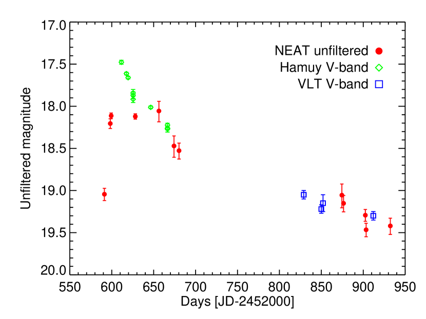
Figure 1: The unfiltered optical light curve of SN 2002ic as observed by NEAT with the Palomar 1.2-m and Haleakala 1.2-m telescopes (see Table 1). The magnitudes have been calibrated against the USNO-A1.0 POSS-E stars in the surrounding field. No color correction has been applied. Also shown are the observed V-band magnitudes from Hamuy et al. (2003) and V-band magnitudes from the spectrophotometry of Wang et al. (2004).

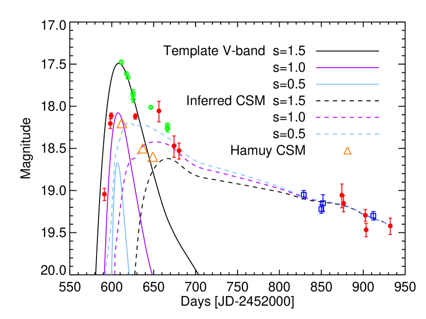
Figure 2: A template SN Ia V-band light curve (solid lines – stretch decreases from top to bottom line) shown for comparison with the photometric observations at several stretch values, $s$, where the magnitude-stretch relation $\Delta m=1.18~{}(1-s)$ has been applied. The difference between the observed photometry points and the template fit has been smoothed over a $50$-day window (dashed lines). Note that an assumption of no CSM contribution in the first $15$ days after maximum light (i.e. $s=1.5$) is in conflict with the spectroscopic measurements of Hamuy et al. (2003) (open triangles–no error bars available).

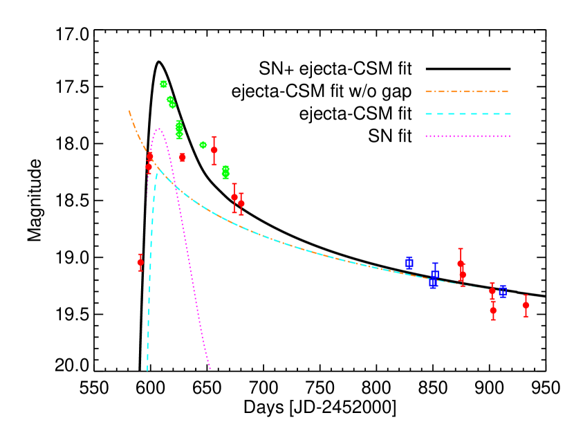
Figure 3: The observed photometry compared with the SN + power-law ejecta-CSM model described in Sec. 6.

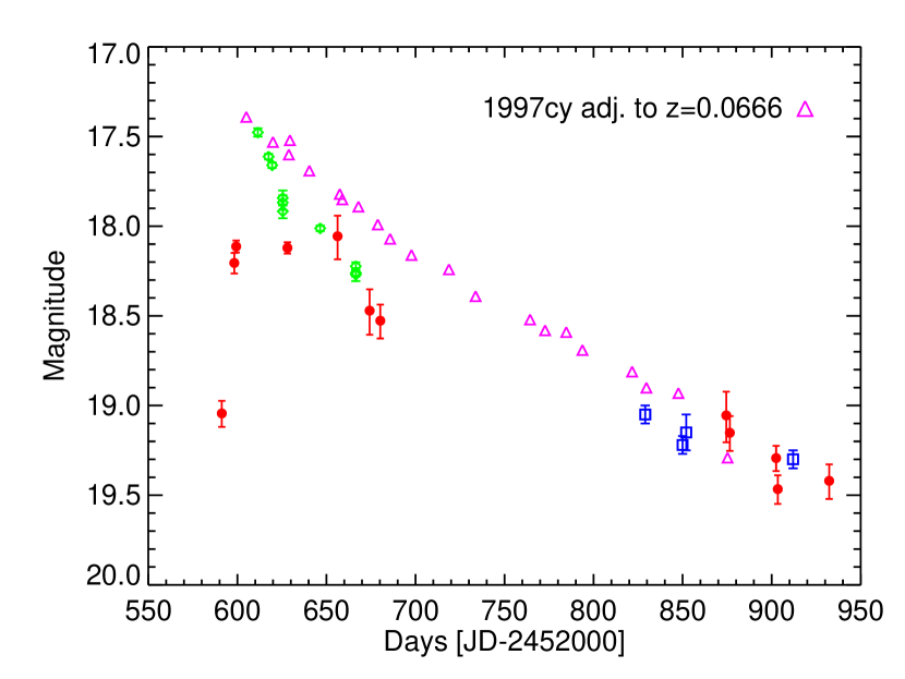
Figure 4: The NEAT unfiltered and Hamuy V-band observations of SN 2002ic compared to the K-corrected V-band observations of SN 1997cy from Germany et al. (2000). No date of maximum or magnitude uncertainties are available for SN 1997cy. Here the maximum observed magnitude for SN 1997cy has been adjusted to the redshift of 2002ic, z=0.0666 (Hamuy et al. 2003), and the date of the first light curve point of SN 1997cy has been set to the date of maximum for SN 2002ic from our V-band fit.

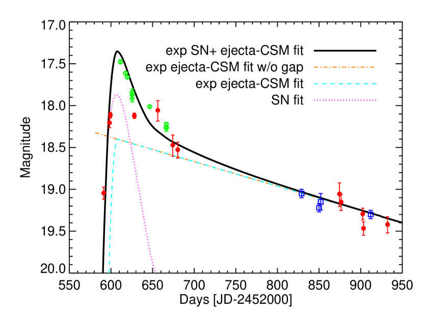
Figure 5: The observed photometry compared with the SN + exponential ejecta-CSM model described in Sec. 7.

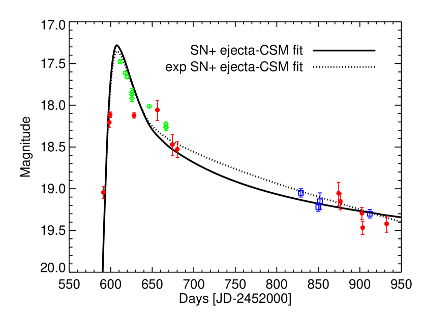
Figure 6: A comparison of fits with power-law (solid) and exponential (dotted) SN ejecta density profiles.

Part 4 Summary

Chapter 7 Conclusions and Future Directions

The Nearby Supernova Factory is poised to change the way we look at Type Ia supernovae. The search pipeline that was developed as the focus of this dissertation will allow for the discovery and subsequent follow-up of $100$ SNe Ia per year out to a redshift of $z=0.1$. At the end of three years, the SNfactory will have studied $300$ SNe Ia in unprecedented detail and will be able to answer many of the questions regarding unknown systematics and variation of SNe Ia maximum magnitudes. In addition, the SNfactory data set will provide an ideal resource to search for improved luminosity distance indicators from SNe Ia.

The pilot test of the SNfactory search pipeline discovered 83 new supernovae and found a total 99 supernovae (Chapter 4). The automated search pipeline currently reduces $30,000$ images a night to less than $100$ subtractions that need to be scanned by a trained scientist. The SNfactory search pipeline has already proven its ability to search on three different detector-telescope combinations (Chapter 2). Additional searching resources could be easily integrated into the pipeline to expand or, if necessary, replace the current data stream. Close integration of the SNfactory discovery and follow-up pipelines will allow for automated discovery and observation of SNe Ia discovered soon after explosion. The SNIFS instrument, custom-designed and built for the SNfactory project, has been commissioned and has begun to observe supernovae found using the SNfactory search pipeline.

The successful prototype run of the SNfactory search pipeline demonstrates that a large automated supernova search can be constructed to find the 100 nearby SNe Ia per year required by the SNfactory science goals. Improvements in star masking, detection of detector artifacts, and image quality standards were all required to reduce the number of subtractions that had to be examined by human scanners. Problematic issues in processing such large amounts of data (60 GB/night) and coordinating large number of jobs on computing clusters were identified and addressed. A salient technical lesson learned was the difficulty in simultaneously accessing a large number of images stored on centralized disk vaults. The storage of images, both locally and on archival storage quickly became a limiting bottleneck. Data management issues such as these will impact future high-volume supernova experiments such as LSST and SNAP.

By their nature, supernova searches are sensitive to contrast against the host galaxy. The SNfactory prototype search and subsequent calculations of rates from the search reveals the significant effect a minimum percent increase requirement has in reducing the number supernovae found (Chapter 5). As the percent increase cut is not applied in the higher-redshift work of the SCP, this effect only applies to the SNfactory work presented here. In retrospect, the magnitude of this effect is apparent, but this experience offers a general lesson on the importance of simulations in predicting and checking the performance of large-scale, automated programs.

The subtraction code used by the SNfactory should be improved to yield fewer false candidates. Explorations of more sophisticated convolution kernels, such as that of Alard & Lupton (1998), are one promising route toward reducing the number of non-astrophysical detections in the SNfactory subtractions. An exploration of additional candidate quality metrics and multi-dimensional score cuts should be pursued to reduce the number of non-supernova candidates currently passed by the automated search scanning software.

The automated, large-sky survey of the SNfactory search has provided a well-defined basis for a calculation of SN Ia rates (Chapter 5). The analysis presented here is the first to measure the efficiency and control time of a multi-epoch supernova search in a truly self-consistent manner. A study of a sample of the tens of thousands of square degrees searched during the fall of 2002 and spring of 2003 yielded a 90% confidence interval for the SN Ia rate of $3.67\ _{-1.66}^{+1.20}\mathrm{(stat)}\ _{-0.11}^{+0.11}\mathrm{(sys)}~{}h^{3}\times 10^{-4}$ SNe Ia/yr/Mpc³, or $1.07\ _{-0.48}^{+0.35}\mathrm{(stat)}\ _{-0.03}^{+0.03}\mathrm{(sys)}~{}h^{2}$ SNu, from a sample of $7.75$ effective SNe Ia, in general agreement with previous studies of nearby SNe Ia. This analysis highlighted the importance of a full understanding of the detection efficiency of the search pipeline. In addition, the effect of the underlying galaxy population light on the search selection criteria was realized and accounted for using a comprehensive sample of galaxies from the SDSS. Supernova searches at higher redshifts will require comparable galaxy catalogs to properly measure the search sensitivities and progenitor populations. The techniques outlined in this dissertation should establish a new standard for calculating SN rates from supernova searches.

In the first year of operation, the SNfactory will easily double the number of supernovae found using its well-characterized search pipeline. The supernovae discovered in the full operational phase of the SNfactory will allow for an improved measurement of supernova rates because all promising candidates will have spectroscopic observations to confirm or reject the new object as a supernova. This extended sample will provide better coverage of supernovae in low-surface-brightness galaxies as well as statistics on supernova types as a function of host galaxy type.

The method of calculating SN rates described in Chapter 5 should be extended to cover the full SNfactory sample. Additionally, an investigation of the SN rate of non-Type Ia SNe would provide a perfect complement to the SN Ia rate from the SNfactory. Core-collapse SN rates are desirable as they are a direct tracer of the star formation history of galaxies. The time delay between stellar formation and SN Ia explosions can be measured by comparing the relative rates of SNe Ia and core-collapse SNe. This delay can offer further hints toward the nature of the progenitor systems of SNe Ia.

In several years, when the SNfactory search data will provide QSO time variability baselines from a week to almost 8 years, the QSO variability investigation presented in Appendix 9 should be revisited in collaboration with those currently working with QSOs as part of the Palomar Consortium. The expanded range of time baselines from further years of the survey will allow for a well-constrained integration of the observed QSO power spectrum with existing QSO variability studies.

Several unusual supernovae that challenge conventional classification were found by the SNfactory prototype search. One of these, SN 2002cx, is a SN Ia that exhibits SN 1991T-like spectral features but is under-luminous like SN 1991bg (Li et al. 2003). Studying category-spanning SNe Ia like SN 2002cx is important in understanding the true diversity of SNe Ia. Perhaps the most interesting supernova found in the initial search was SN 2002ic. This supernova was the first SN Ia to exhibit hydrogen emission lines (Hamuy et al. 2003). This emission, together with a highly elevated light curve for at least a year after explosion, was interpreted as evidence for circumstellar material surrounding the progenitor system of SN 2002ic. This material has a density structure consistent with a post-AGB star that has just ended its final mass-loss phase. Several other previously observed supernovae were proposed to be possibly related to SN 2002ic. This identification of a specific period in the evolution of the stellar system of SN 2002ic offers a unique insight into the progenitors of SNe Ia. Both SN 2002cx and SN 2002ic highlight the importance of surveying the entire population of SNe Ia to understand the behavior and origin of these invaluable cosmological tools.

The final comprehensive SNfactory spectrophotometric data set on 300 SNe Ia will allow for a wide range of studies of SN Ia phenomenology and physics. In particular, investigations into correlations between spectral features and luminosity distance indicators should yield improvements in cosmological measurements using these important standardizable candles. This analysis should be done at yearly intervals and eventually lead to a final analysis after the last final reference spectrum is taken. The wealth of data to be accumulated by the SNfactory should occupy future graduate students for years to come.

Part 5 References

Part 6 Appendices

Chapter 8 SNfactory Summary

[The following appeared in New Astronomy Review as Wood-Vasey et al. (2004a).]

Appendix 8.A Abstract

The Nearby Supernova Factory (SNfactory) is an ambitious project to find and study in detail approximately 300 nearby Type Ia supernovae (SNe Ia) at redshifts $0.03<z<0.08$. This program will provide an exceptional data set of well-studied SNe in the nearby smooth Hubble flow that can be used as calibration for the current and future programs designed to use SNe to measure the cosmological parameters. The first key ingredient for this program is a reliable supply of Hubble-flow SNe systematically discovered in unprecedented numbers using the same techniques as those used in distant SNe searches. In 2002, 35 SNe were found using our test-bed pipeline for automated SN search and discovery. The pipeline uses images from the asteroid search conducted by the Near Earth Asteroid Tracking group at JPL. Improvements in our subtraction techniques and analysis have allowed us to increase our effective SN discovery rate to $\sim$12 SNe/month in 2003.

Appendix 8.B Introduction

Type Ia supernovae (SNe Ia) have proven extremely useful as standardizable candles to explore the expansion history of the Universe (Perlmutter 1997; Perlmutter et al. 1998; Garnavich et al. 1998; Riess et al. 1998a; Perlmutter et al. 1999). Ambitious follow-on experiments are just starting, SNLS (Pain & The SNLS Collaboration 2003), ESSENCE (Garnavich et al. 2002), or have been planned, SNAP (Aldering et al. 2002b), to extend the revolutionary result that the Universe is accelerating to precise statements about the constituents and history of the Universe. However, a key assumption underlying these experiments is that the current observed diversity in SNe Ia will be well-behaved and calibrated to allow for the desired precision measurements. This assumption can be tested in large part using nearby SNe Ia. Moreover, there is the possibility for such nearby studies to uncover new relationships that will make SNe Ia even better standard candles, much as the width-luminosity relation has brought SNe Ia to their already impressive level of standardization.

The Nearby Supernova Factory (SNfactory) project is designed to bring this improved understanding of SNe Ia (Aldering et al. 2002a; Pécontal et al. 2003; Lantz 2003). Over the course of three years, it will study 300 SNe Ia in the nearby smooth Hubble flow 2. These SNe will be observed with a dedicated instrument, the SuperNova Integral Field Spectrograph (SNIFS), which is currently in the final stages of construction. SNIFS will provide simultaneous spectrophotometric coverage of both the SN and the host galaxy at 3–5 day intervals during the rise and fall of each SN. This unprecedented dataset will provide a wealth of information on SNe Ia and allow for an improved calibration of SNe Ia for use in cosmology.

Appendix 8.C The Supernova Search Dataset

The SNfactory searches for SNe using wide-field images obtained in collaboration with the Near Earth Asteroid Tracking (NEAT) group (Pravdo et al. 1999) at the Jet Propulsion Laboratory (JPL). In their quest for asteroids, the NEAT group observes hundreds of fields each night by taking three images of each field, spaced fifteen to thirty minutes apart, and searching for objects that move by more than a couple of arcseconds over this period. The SNfactory uses this temporal spacing to eliminate asteroids and reduce cosmic-ray contamination. The NEAT observing program covers the observable sky from $-40$ to $+40$ degrees in declination every one to two weeks.

Since 2001, the Palomar 1.2-m. Oschin telescope has been used by the SNfactory-NEAT collaboration. The NEAT group outfitted this telescope with an automated system for control and observations and added a 3-chip, 3 $\sqcap$$\sqcup$^∘ field-of-view CCD camera (NEAT12GEN2) at the spherical focal plane of this Schmidt reflector. We spent 2001 designing, testing, and verifying the search pipeline with the large data stream from this telescope. Full search operations began in the fall of 2002 and continued through April of 2003 when the NEAT12GEN2 camera was replaced by the Yale QUEST group (The QUEST Collaboration 2003) with a 112-chip, 9 $\sqcap$$\sqcup$^∘ field-of-view camera (QUESTII) capable of both drift-scan and point-and-track observations. QUESTII became operational in August 2003 and is now providing data for the SNfactory search. The NEAT group also uses the Haleakala 1.2-m MSSS telescope, but as this telescope has a smaller field of view and poor image quality, the SNfactory has focused its search efforts on the images from the Palomar Oschin telescope.

Appendix 8.D Data Processing

The SNfactory, in collaboration with the High Performance Wireless Research and Education Network (Braun 2003), has established a high-speed, 6 Megabyte-per-second (MBps) radio internet link to the San Diego Supercomputer Center (SDSC) from the Palomar observatory. Images are transmitted from the telescope and stored at the National Energy Research Supercomputing Center (NERSC) High Performance Storage System (HPSS). The bandwidth from SDSC to NERSC allows for near real-time transfer of 20–50 GB per night. From HPSS the data are transferred to the 200-node NERSC Parallel Distributed Systems Facility (PDSF) and are submitted for simultaneous processing on the PDSF cluster in groups based on the dark frame taken closest in time. The processed images are then registered with our image database, renamed to match our canonical name format, and saved to HPSS.

The SNfactory searches these data for SNe using image subtraction. The computers use a sophisticated suite of image tools, but there remains a significant, although ever-decreasing, amount of human interpretation needed to discriminate the good SN candidates from the bad. The same software used by the SNfactory to search for nearby (z $\leq 0.1$) SNe is used by the Supernova Cosmology Project (SCP) to search for distant SNe. Our subtraction software begins by spatially registering all of the images of a given field to a common reference system. The images to be used as a reference are stacked into a single coadded image, while the images to be searched are coadded into two separate images to allow for later checks for asteroids and cosmic rays. To account for differences in the effective point-spread-function from variations in atmospheric and telescope conditions, we calculate a convolution kernel to match each coadded image to the worst-seeing coadded image of the set. An automated scanning program looks for objects in the convolution-matched, subtracted image and applies a variety of selection criteria to eliminate cosmic rays, asteroids, and subtraction and detector artifacts. This program compiles a list of interesting candidates to be looked at in more detail by a human scanner. Every day, human scanners consult the list of interesting candidates and decide whether or not a computer-flagged candidate appears to be a real, variable object. Once we have a promising candidate, we submit it to the target list for the next night of observation with NEAT. After obtaining confirmation images of a candidate that reveal it to exhibit the appropriate behavior for a SN, we announce the apparent SN in the IAU Circulars. A confirmation spectrum is desirable but currently not always possible. When the SNIFS instrument is installed on the Hawaii 2.2-m telescope, it will be automatically scheduled to confirm and follow SNe. Spectra will be taken of each SN at 3–5 day intervals over a span of roughly 60 days.

Appendix 8.E Results

Eighty-three SNe have been found using the techniques described above and have been accepted by the International Astronomical Union. Fig. 1 shows the 35 SNe we discovered in 2002. In the first five months of 2003, we found and reported an additional 48 SNe. In addition, our search identified another 17 SNe that had already been reported by other groups. We are currently running with a very conservative set of selection criteria and need human eyes to scan $\sim 5$% of the successful subtractions for each night. However, many of the SNe discovered in 2003 could have been found using very restrictive criteria that would have required human scanning for $<1$% of the subtractions. To further reduce our scanning burden, efforts are ongoing to understand the parameter space of our candidate scores to uniquely identify the SNe.

In order to understand our search results, we have developed a simple search simulator. We use a V-band lightcurve template from Goldhaber et al. (2001) to model the rise and fall of SNe Ia. The simulator calculates the amount of time a supernova would be visible at a given redshift assuming a normal (stretch $=1$) SN Ia. We considered a redshift range from $0<z<0.2$, a limiting unfiltered magnitude of 19.5, and several different repeat coverage cadences for our simulations. We included the typical NEAT sky coverage rate, $S_{D}=500~{}\hbox{\hbox to0.0pt{$\sqcap$\hss}$\sqcup$}\hbox{${}^{\circ}$}$/night, and assumed $S_{O}=$10,000 $\sqcap$$\sqcup$^∘ of usable sky a night. There is a maximum effective cadence, $C_{\mathrm{max}}$, beyond which one is just idling the telescope: $C_{\mathrm{max}}=S_{O}/(S_{D}-\frac{S_{0}}{365~{}\mathrm{days}})$. For the NEAT observation program, this cadence is approximately 20 days.

An important goal of the SNfactory is to discover SNe early enough after explosion to follow them through their rise and fall. Fig. 3 shows a comparison of our simulations of the SNe discovery phase with the actual discovery phase for SNe from the SNfactory search having well-known dates of maximum. For shorter sky coverage cadences less sky can be covered and so fewer SNe are discovered overall, although the epoch of each SN can be better constrained. Fig. 3 clearly shows that the SNfactory search pipeline is successfully finding SNe Ia early in their lightcurves.

Appendix 8.F Conclusion

The Nearby Supernova Factory search pipeline is operational and has proven the ability to discover $\sim 12$ SNe/month $\Rightarrow$ $\sim$150 SNe/year. As $\frac{2}{3}$ of the supernovae discovered in our search have been SNe Ia, we expect to discover $\sim 100$ SNe Ia/year. Most of these supernovae have been discovered sufficiently early to enable detailed study starting before maximum light. This extensive study will enable improvements in the use of SNe Ia for cosmological measurements, and provide a wealth of information on the supernovae themselves.

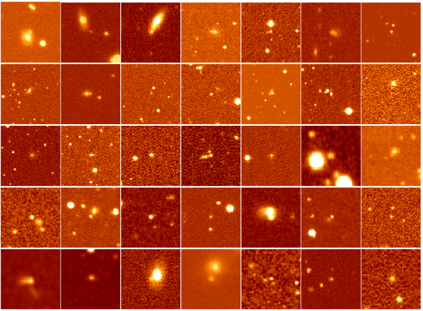
Figure 1: A mosaic of the 35 supernovae found by the Nearby Supernova Factory pipeline in 2002. Each image is centered on the respective supernova.

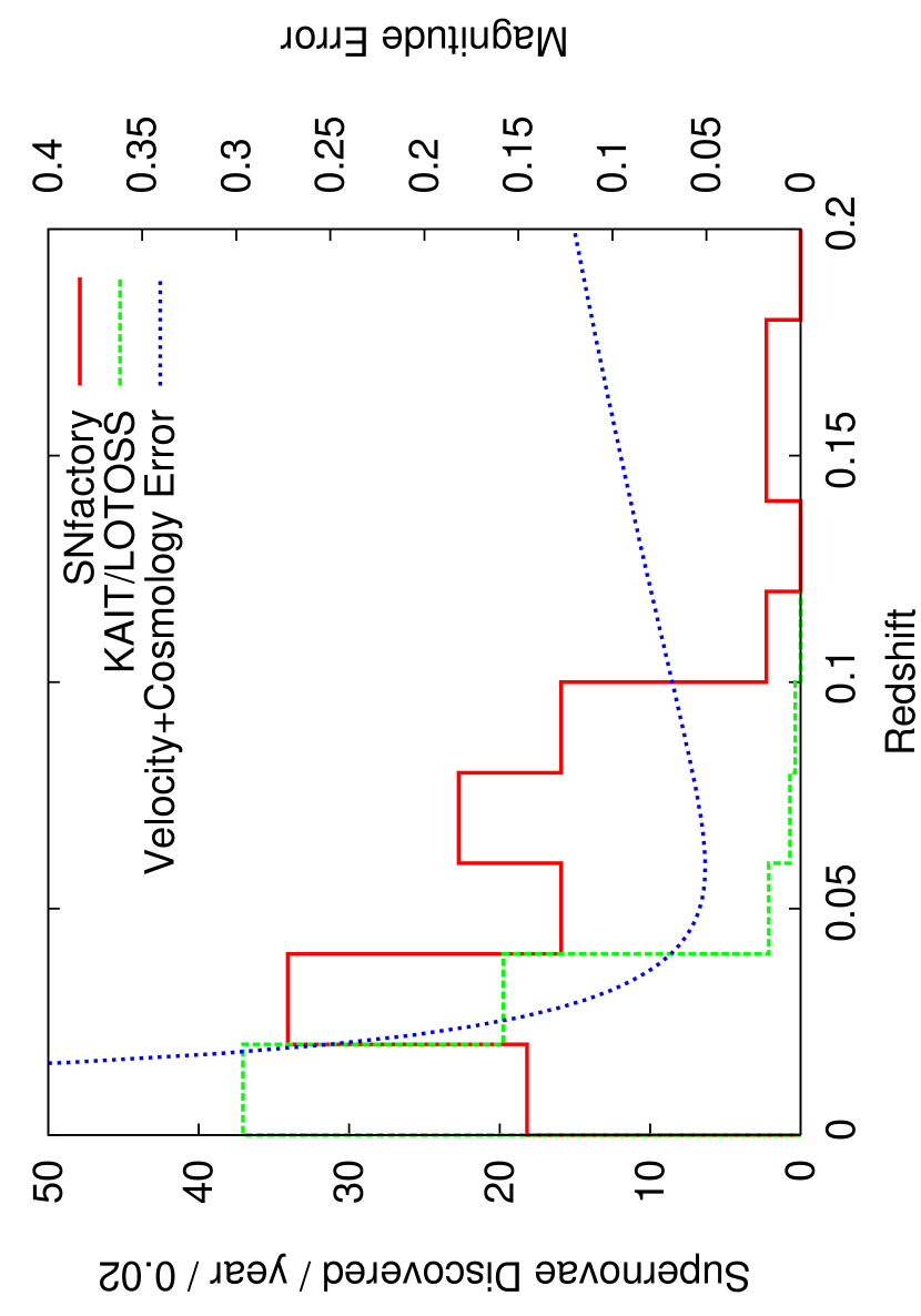
Figure 2: The SNfactory is operating in the “sweet spot” redshift range between peculiar-velocity noise and cosmological uncertainty. The SNfactory curve is the redshift distribution of supernovae found and spectroscopically confirmed in our search to date scaled up to 100 SNe/year. The velocity error is for an assumed $300$ km/s velocity dispersion. The cosmology error is modeled as the difference between an Einstein-de Sitter cosmology and a Universe with $\Omega_{M}=0.3$ and $\Omega_{\Lambda}=0.7$.

Figure 3: The distribution of discovery epoch for the SNe Ia with determined dates of maximum found in the SNfactory dataset compared with the simulations described in the text. The model curves are not calculated in absolute units and have been scaled for comparison with the observations. As the model curves show, a shorter cadence gives fewer supernovae but better constraints on the epoch at discovery.

Chapter 9 QSOs and Microlensing

Appendix 9.A Introduction

Quasi-stellar objects (QSOs) were discovered by Sandage and Mathews over forty years ago (Sandage 1961; Burbidge 1967; Schmidt 1969) and were eventually understood as a class of active galactic nuclei (AGN) (Antonucci 1993). Due to historical convention, there are a variety of names for these AGNs according to the different observed properties: quasars (radio-loud and radio-quiet), X-ray galaxies, Seyfert galaxies, low ionization nuclear emission region (Liner) galaxies, and broad absorption line objects (BALs). The “quasar” designation has generally been used for unresolved, point-like objects, while the various galaxy classifications have been assigned when there is a resolved object. But all of these classifications share the common model of a massive central engine that powers energetic radiation that is subject to variability over both short and long time scales. I will refer to the general class of these objects as QSOs in this study.

QSOs have been known to exhibit variability in their flux since soon after their discovery (Burbidge 1967; Schmidt 1969; Wagner & Witzel 1995; Ulrich et al. 1997). This variability could be due to causes either intrinsic or extrinsic to the active galactic nucleus itself. One possible candidate for a source of extrinsic variability is microlensing by compact objects between the QSO and the observer (Schneider 1993). Schneider (1993) presented work constraining the composition of possible compact objects given the observed statistical variations in the lightcurves of QSOs. Zackrisson & Bergvall (2003); Zackrisson et al. (2003) (hereafter referred to as ZBZ) found that a microlensing model could explain the observed average structure function of QSOs, but that it did not explain the scale of variability for nearby QSOs ($z<1$) or the high variability ($>0.35$ mag) at any redshift. They concluded that while microlensing may be a possible explanation for some part of the observed QSO variability, there must be another mechanism, possibly intrinsic, at work to explain all of the observed fluctuations. ZBZ focused on QSO variability on the scale of one-to-ten years and averaged over smaller, intra-year variability. The NEAT dataset provides a new opportunity to investigate variations on the time scale of a week to a few years. This chapter details the results of an investigation of this relatively unexplored region of the QSO time-variability power spectrum.

Appendix 9.B The NEAT data set

The NEAT data was originally analyzed for QSO variability by Roland Rudas for his senior thesis in Physics at UC Berkeley (2003). He analyzed $229$ QSOs visible in the NEAT survey and developed initial numbers on the $\Delta t$ vs. $\Delta m$ distribution. I have built on that work by extending the QSO sample to 982 objects, computing the time-variability power spectrum from the light curves, calculating the variation amplitude probability density function and investigating the effect of a median versus mean algorithm for computing the power spectrum and other measures of variability.

Appendix 9.C QSO Catalogs

The QSO catalogs of Véron-Cetty & Véron (2001) (VC01) and Schneider et al. (2003) (S03) were used as the source of QSOs for this work. The $40,473$ QSOs presented in these catalogs ($23,760$ from VC01 plus $16,713$ from S03) were checked against the NEAT dataset for QSO variability. Out of those $40,473$ QSOs, 3131 were covered by images from the NEAT survey and were brighter than $V<20$ (VC01) or $g<20$ (S03). Requiring a signal-to-noise $\geq 5$ for each light curve points (see below), left a final total of 982 QSOs for this analysis.

Appendix 9.D QSO Photometry

For each QSO matching the criteria above, all of the NEAT images covering its coordinates were retrieved from long-term storage on the NERSC HPSS system (see Chapter 2) and and calibrated against the USNO-A1.0 catalog (Monet et al. 1996) “R”-band magnitudes. While the USNO-A1.0 catalog suffers from plate-to-plate uncertainties of $0.2$ magnitudes (see Appendix 10 for more details on the NEAT calibration), this should not affect the results presented here as this is a differential analysis and all of the NEAT images of a given QSO substantially, if not completely, overlap with the same plate—each POSS plate is $6.5\hbox{${}^{\circ}$}\times 6.5\hbox{${}^{\circ}$}$ while the NEAT images are at most $0.25$^∘ on a side—so the relative calibration for a given QSO is almost always derived from within the same POSS plate. Each image was photometered using aperture photometry scaled to the observed x- and y-FWHM measured for the image. No extinction corrections were performed. The magnitudes measured from all of the images for a given QSO were saved in a light curve file for the QSO for later analysis.

In the analysis of the light curve properties, data from the same night was medianed together. This median step was served to eliminate outliers derived from bad images. As most observations were from triplets of images during a given night, a good data point was obtained for most nights of observation. Fig. 1 shows a scatter plot of $\Delta f$ versus $\Delta t$. Figs. 2 & 3 show the one-dimensional histograms from Fig. 1 for $\Delta t$ and $\Delta f$, respectively. Figs. 4, 5, 6, and 7 show the power spectrum histogram for $\Delta f$. See Fig 9 for a histogram of the magnitude fluctuations observed in my sample.

Appendix 9.E Power Spectrum of QSO Variability

A generalized analysis of variability naturally leads to a power-spectrum analysis. The flux of the variability at each time scale is often a predicted characteristic of modeling of the phenomenon. As QSO variability is poorly understood, a power spectrum analysis is a useful way of comparing different physical models whose effect on the power-spectrum can be calculated theoretically. ZBZ present their results in the context of a power spectrum. Fig. 4 and Fig. 5 show the QSO structure function as calculated from the NEAT light curve using Eq. 2 of ZBZ (rewritten as Eq. 1 in this text). The QSO structure function, $S(\tau)$, is defined as

$$S(\tau)=\sqrt{\mathrm{mean}\left(\Sigma_{i<j}\left(m_{j}-m_{i}\right)^{2}\right)}$$ (1)

$$S(\tau)=\sqrt{\mathrm{median}\left(\Sigma_{i<j}\left(m_{j}-m_{i}\right)^{2}\right)}$$ (2)

ZBZ calculated the average structure function by taking the average of Eq. 1 over each QSO. This approach suffers the disadvantage of weighting all of the QSOs used in the analysis equally even if they have significantly different numbers of data points in their lightcurves. For the ZBZ analysis, their coverage relatively homogeneous and so this was less of an issue. In the analysis of the NEAT data, the number of data points contributed by each QSO varied significantly so I chose to consider all of the $\Delta t$ and $\Delta f$ values together and calculated my statistics treating each of those pairings equally. Since I am testing the hypothesis that QSO variability is caused by microlensing events, which are caused by physical conditions uncorrelated from the QSOs, this treatment is valid.

Statistical comparisons of $\Delta f$ versus $\Delta t$ and $m$ versus $\Delta t$ were made for each QSO where

$$\Delta f = \frac{f_{j}}{f_{i}}$$ (3)

$$\Delta m = -2.5\log_{10}{\Delta f}$$ (4)

$$\Delta t = t_{j}-t_{i}$$ (6)

$$\forall~{}i<j.$$

A total of of 20309 measurements and 49489 differences were obtained from this process.

Appendix 9.F Discussion

My work presented here shows a QSO power spectrum consistent with some of the microlensing models analyzed in ZBZ to time scales down to a week on a slope that matches that found by ZBZ for time scales of 1–20 years. Figs. 4 & 5 show the results of my power-spectrum analysis for the mean and median amplitudes. The difference between taking the mean (Eq. 1) versus median value (Eq. 2) in the calculation of the structure function is clear. Fig. 9 show a histogram of the distribution of $\Delta m^{2}$ along with the mean and median of the distribution. The difference between these numbers for the entire sample accounts for the difference in the two methods of calculating the structure function. Fig. 8 shows the ratio of Fig. 4 and Fig. 5 and the expected offset from a Gaussian distribution (green line) and the actual distribution of $\Delta m^{2}$ (blue line). To compare with the results of Zackrisson et al. (2003), I show the mean structure function in Figs. 4 & 6, but I wish to point out the significant weight that large variations have on the average magnitude fluctuation and the difficulty in assigning a meaningful error bar to the mean given the distribution shown in Fig. 9. Thus, for the rest of the analysis, the median value will be used.

The power-spectrum slope of (Zackrisson et al. 2003) is indicated in Figs. 6 & 7. Note that the solution from ZBZ has a slope completely consistent with the analysis presented here. This slope is a major factor in determining the source of QSO variability and its continuation to smaller time scales is consistent with a range of microlensing models considered by ZBZ. These studies do not entirely overlap as my survey has a smaller baseline and fewer data points at larger time gaps. This different time baseline coverage was a large part of the motivation for undertaking this study. However, my larger and differently biased QSO sample may also be part of the explanation for the difference observed in the region from 1 to 3 years.

Zackrisson et al. (2003) stated that Hawkins observed a dispersion of $0.13$ magnitudes from the intra-year plates and thus they estimated that the contribution on these time scales was an uncorrelated $\sigma_{m}=0.065$. Assuming the use of the term “dispersion” means standard deviation of the distribution without any relative uncertainty weighting, I observe a significantly higher standard deviation of $0.52$ magnitudes for my sample of time baselines less than one year. This is not too different from the $0.65$ magnitudes seen in my sample of time baselines greater than one year and is comparable to the $0.57$ magnitudes seen for my overall sample.

The smaller time-gap region also shows a flatter slope than that found by (Hawkins 2002) or ZBZ. As Zackrisson et al. (2003) note, this is consistent with microlensing from objects of mass $M_{\mathrm{compact}}<10^{-5}~{}M_{\odot}$. ZBZ argued against this possibility as such a small slope and thus relatively higher power at small scales was inconsistent with their observed structure function. However, the structure function I present here shows more power on small time scales and is consistent with the small slope expected from microlensing.

Figure 1: A scatter plot of $\log_{10}{\Delta f}$ versus $\Delta t$ from the QSOs covered in the NEAT dataset.

Figure 2: Histogram of observed time baselines, $\Delta t$.

Figure 3: Histogram of observed relative change in flux, $\Delta f=\frac{f_{j}}{f_{i}}$.

Figure 4: The QSO average structure function (as defined in Zackrisson et al. (2003)) derived from an analysis of the QSOs in the NEAT dataset. The error bars are computed as the standard deviation from the mean of the $\Delta f$ distribution.

Figure 5: The QSO median structure function (as in Fig. 4 but using a median instead of average on the change in magnitude) derived from an analysis of the QSOs in the NEAT dataset. The error bars are computed based on including $\pm$34% of the area around the median.

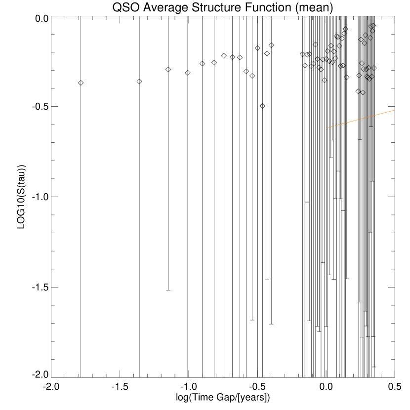
Figure 6: Fig. 4 plotted in log space. The line in orange is the power-spectrum slope of ZBZ.

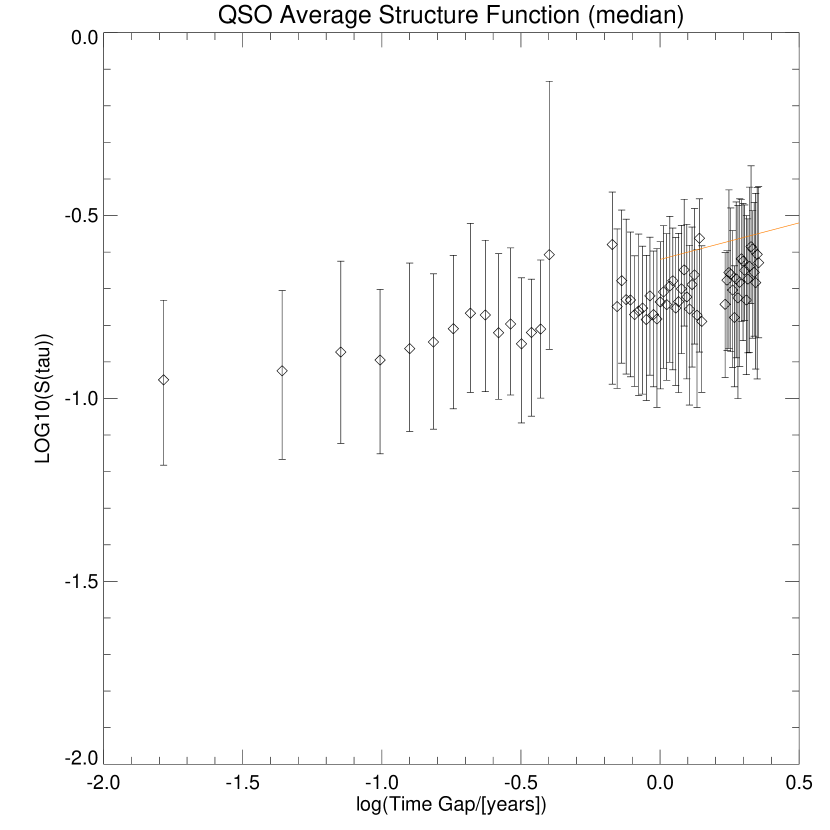
Figure 7: Fig. 5 plotted in log space. The line in orange is the power-spectrum slope of ZBZ.

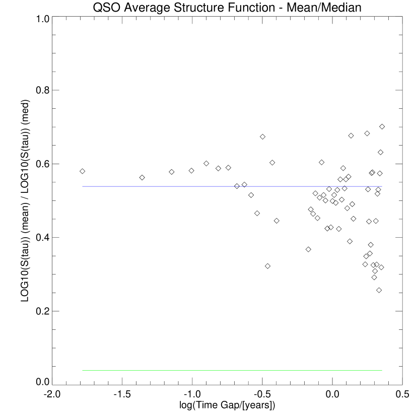
Figure 8: The ratio of the QSO structure function as calculated using the mean versus median of flux change values.

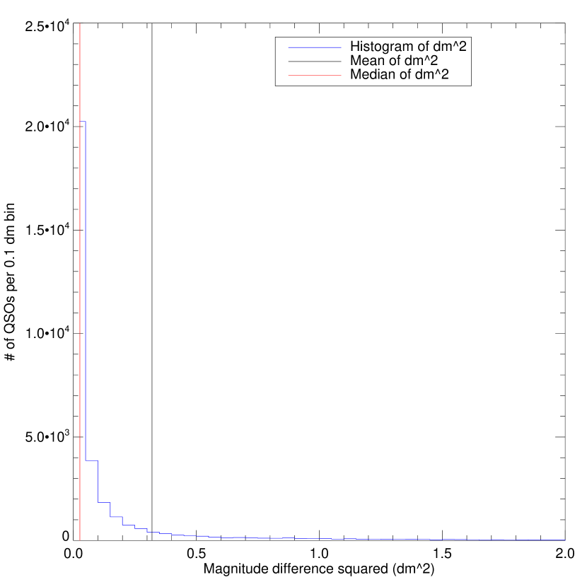
Figure 9: The distribution of magnitude fluctuations for all time scales. Note the significant difference between the mean (black line) and median (red line) of the distribution.

Figure 10: The cumulative probability amplitude distribution for my QSO sample. This plot varies significantly from that of Zackrisson et al. (2003) and is more consistent with the microlensing models presented therein.

1 Cumulative Probability Amplitude

Zackrisson et al. (2003) also compare the cumulative probability amplitude distribution of their sample with models. I obtain a very different distribution than ZBZ at both small and large time scales. Fig. 10 shows a smoothly increasing concave curve without any sharp cutoff or significant inflection point as seen in Figs. 3 & 4 of Zackrisson et al. (2003). There is no large cutoff at $0.35$. Rather, 40% of objects have a variability less than $\delta m=0.35$. This allows a range of models from Fig. 5 of Zackrisson et al. (2003). Note that the modeling of observational uncertainties can be important in considering small-scale variability. Zackrisson et al. (2003) include the error of the measurements in their models. This makes it difficult to truly compare my sample with different error bars to the models they show in their paper. However, the power observed on small scales in this analysis is much larger than the observational uncertainties.

2 QSO amplitude redshift dependence

Fig. 13 shows the distribution of QSO mean amplitude,

$$\delta m=\mathrm{max}(m(t))-\mathrm{min}(m(t))$$ (7)

versus redshift. The error bars represent the standard deviation of the sample in each redshift bin. There is a large degree in uncertainty in these values and the distribution itself is highly non-Gaussian around the calculated mean as can be seen in Fig. 14. Fig. 13 is the analogous plot to Fig. 6 of Zackrisson et al. (2003) where they note their error bars as “the uncertainty in the position of the observed mean,” which we take to mean that they were using the error in the calculation of the mean and not the standard deviation of the distribution. For a distribution such as that shown in Fig. 14, the quoted error bars in Fig. 6 of Zackrisson et al. (2003) would seem misleading in my analysis.

In addition, for my sample, the $\delta\,m$ statistic of Eq. 7 is not a good statistic as my light curve is inhomogeneous and thus QSOs with more observations are more likely to have larger values of $\delta\,m$. In general $\delta\,m$ is a quantity dependent on the observational program. I prefer an analysis of the median difference for each QSO, as shown in Fig. 12. If this statistic can be compared with Fig. 6 of Zackrisson et al. (2003) then my results are consistent with the microlensing models with characteristic variability amplitudes of $0.2$ and are not a strong function of redshift. This flat dependence of variation amplitude with redshift is consistent with the findings of Hawkins (2000).

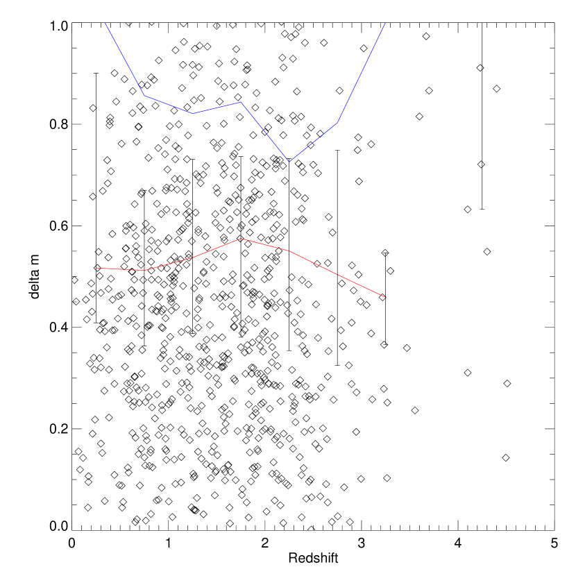
Figure 11: A scatter plot of mean amplitude (Eq. 7) versus redshift for the QSOs in this analysis. Binned version of the data is shown by the over-plotted lines. The blue line is the mean, while the red line is the median of the distribution. The standard deviation of the points in each redshift bin are shown as errors on the mean line. A similar uncertainty in the median line can be postulated, but note that the distribution of mean amplitudes is not symmetric about the mean value but instead is piled up to zero. Zackrisson et al. (2003) finds a maximum mean amplitude of approximately 0.4 mag at a redshift of $z=0.5$. This is easily consistent with the error bars implied by the distribution of values in the plot.

Figure 12: The median values from Fig. 11. The error bars are from a 68% inclusion of points around the median value.

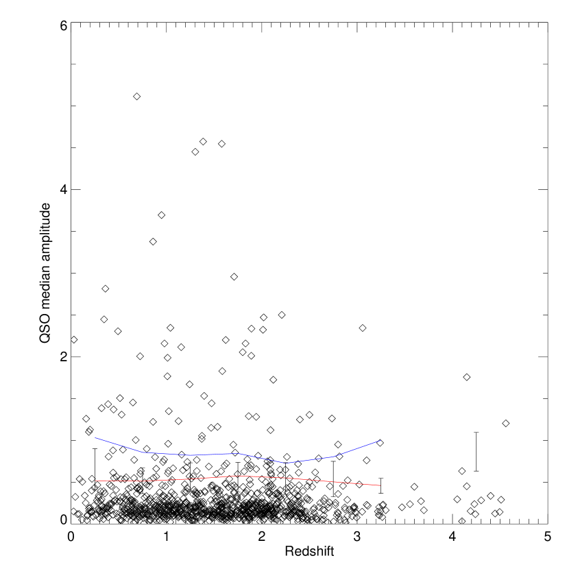
Figure 13: A scatter plot of median amplitude versus redshift for the QSOs in this analysis. Similar to Fig. 11 except uses the median of all of the variability amplitudes for each QSO.

Figure 14: The histogram of mean amplitudes for my QSO sample. Note the concentration near zero. This makes the statistics of Fig. 13 difficult to interpret as a Gaussian distribution.

Appendix 9.G Conclusions

The NEAT QSO sample exhibits an average structure function consistent with that of Hawkins (2002) and ZBZ, but I find significantly different properties in the cumulative probability distribution, the fraction of low-variability objects. My amplitude-redshift relation agrees with Hawkins (2002) but not with ZBZ. These differences generally ease the constraints on the microlensing models used by ZBZ and my results are consistent with a range of QSO microlensing models presented in ZBZ.

Further investigations using an expanded dataset from the NEAT searches will allow a revisiting of these effects and the eventual use of a QSO sample that is an order of magnitude larger than that of Hawkins (2000) and is selected in a different and less-biased way. More sophisticated understanding of the model predictions with regards to the distribution of QSO variability fluctuations around the mean and median distributions is encouraged to standardize the analysis of different QSO-variability datasets.

I conclude that the different selection biases in the two samples and the use of averaging to analyze variability lead to the different results. I am particularly concerned with the low-variability numbers of the Hawkins (2000) sample and find that intra-year variations are significant and comparable to the longer-term variations focused on in ZBZ. Small, $10^{-5}$ $M_{\odot}$, compact objects can provide the observed variability and small slope observed in my sample. Thus I elaborate on the of conclusion Zackrisson et al. (2003) to state that my results are consistent with microlensing as an explanation for the observed variability of QSOs in my sample and allow that if there is another mechanism for variability that it is a longer-scale process that leads to variability on the time scale of years instead of months. This division by time scale of the contributions of different variability mechanisms satisfies some of the more difficult light-travel and energy-transport time problems in many central-engine-based explanations of short-term, achromatic luminosity variations in QSOs, but allows that central-engine variability could dominate QSO variability on longer time scales.

Appendix 9.H Acknowledgments

I would like the acknowledge the significant contributions of Roland Rudas who did the initial study of QSO variability in the NEAT data as part of his senior thesis in Physics at UC Berkeley.

Chapter 10 Calibration of the NEAT System Response

Appendix 10.A Pre-Introduction

This chapter documents attempts to calibrate the NEAT photometric systems. These attempts were largely unsuccessful and are documented here as an aid to future efforts in this direction. The calibration of the NEAT detector systems is discussed in Chapter 6 for the specific case of SN 2002ic. In general, no color calibration was found that yielded improved results over the naïve approach of calibrating NEAT magnitudes off of stars from the “red” USNO A1.0 catalog (Monet et al. 1996).

Appendix 10.B Introduction

The first two NEAT detectors on Haleakala and Palomar were used in an open, unfiltered mode. This choice was made by the NEAT group because asteroids shine in reflected sunlight and an open filter maximizes the amount of light detected from an asteroid. However, it can also let in more light from other sources, most notably the night sky background. In the optical regime, the night sky brightness is mostly due to scattered light and so is blue. Thus an $R$ filter can help reduce the contamination of night sky light and in bright time there is a gain in detection sensitivity. However, in dark time, when scattered light is less of an issue, there is a loss in detection sensitivity due to cutting out more light from the object. These two factors are roughly comparable (Kessler 2002).

After some discussions with the NEAT group, they agreed to observe with a filter when using the new QUESTII camera installed on the Palomar 1.2-m telescope. This could have been a definite advantage for the SNfactory as it would have allowed for calibration of supernova observations against standard filters. Unfortunately, the NEAT group chose to use an RG-610 filter (Fig. 1). While a known filter shape in combination with the measured QE curves for the QUESTII camera will allow for a well-constrained understanding of the effective response function, it won’t be possible to cleanly compare these magnitudes with other observations in more standard filters such as $UBVRI$ or $ugriz$. The filter choice for the NEAT QUESTII observations is currently being reconsidered for summer 2004 operations and beyond.

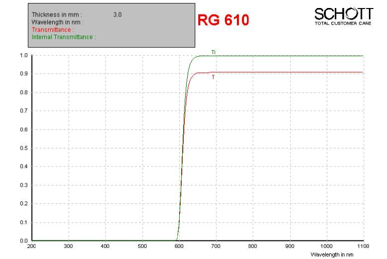
Figure 1: The filter used by the NEAT asteroid search on all four fingers of the QUESTII camera (Bes Optics 2003).

Leaving aside the filter for the new QUESTII camera for the moment, there are years of unfiltered data with one hundred supernovae observed with NEAT detectors and it would be valuable to place this on a known photometric system. This goal requires the calibration of historical NEAT detectors (the Haleakala NEAT4GEN2 and the Palomar NEAT12GEN4) to determine a total effective response of the system as a function of wavelength. This response function depends on a number of factors including the quantum efficiency of the CCD, the optical properties of the telescope and the atmospheric transmission.

Appendix 10.C Calibration Techniques

Two major opportunities for calibration presented themselves: Landolt standard fields (Landolt 1992) and the Sloan Digital Sky Survey (SDSS) (Sloan Digital Sky Survey 2003). Over the course of the past few years of NEAT observations, thousands of images have been taken of a variety of Landolt standards. This extensive and repeated coverage provides the opportunity to determine effective color terms between the Landolt standard stars in $UBVRI$ and the unfiltered NEAT observations. The supplementary work of Stetson (2004) is also available for a more thorough calibration of the Landolt standard fields. The SDSS survey provides five-band $ugriz$ colors for millions of stars. Using the overlap between the SDSS Data Release 1 (Sloan Digital Sky Survey 2003) (SDSS Data Release 2 was not yet released when the work described in this chapter was done), we can thus similarly calculate color terms between $ugriz$ and the unfiltered NEAT observations. Calibration against the Landolt fields has the advantage of directly providing color terms for the $UBVRI$ filters commonly used in supernova work. Calibrating against the SDSS survey is better in all other ways due to the increased sky coverage and far greater number of stars. Some combination of the two would be the best solution.

A general caveat is that color terms between filters can only be defined with respect to an assumed spectral shape. Thus the color terms that can be derived from the comparisons mentioned above are strictly only valid for an archetypical star representing the aggregate of all the stars used in the calibration and are not entirely valid for calibration of supernova lightcurves. This is related to the general problem of S and K corrections so vital to precision photometry but is beyond the precision we can achieve here.

Appendix 10.D SDSS Calibration

The SDSS DR1 provides 88 million objects in $3324$$\sqcap$$\sqcup$^∘ across the sky (Sloan Digital Sky Survey 2004) (see Fig. 2). These stripes overlap with the NEAT coverage pattern (compare Fig. 2 and Fig. 3) in a number of regions and some SDSS field is normally covered during the course of each night’s observations. This is in contrast to the Landolt fields, which are observed more rarely.

Figure 2: The RA and Dec sky coverage of the SDSS DR1 (Sloan Digital Sky Survey 2003).

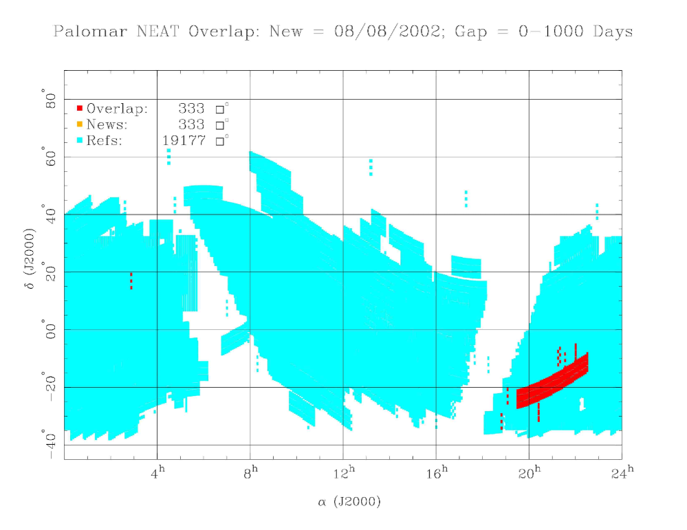
Figure 3: The RA and Dec coverage of the NEAT survey (light coloring) with a sample night of search coverage (dark coloring). This figure is for search images taken the night of 8 August 2002. The nightly sky coverage has since doubled with the new QUESTII camera.

The SDSS color bands are defined in terms of the specific Gunn filters mounted on the Apache Point 2.5-m telescope. The Gunn system is an AB magnitude system where there is no filter-by-filter zeropoint adjustment to match a stellar spectrum. Only one color zeropoint is set and the rest just come from the $\log{\mathrm{flux}_{\mathrm{filter}}}$ relative to the nominal $\log{\mathrm{flux}}$ value. By contrast, in the Vega system a model of the star Vega is defined to have a color of 0 in each filter $UBVRI$. This is clearly different from what one would get from just taking the $\log$ of the flux as flux increases and decreases with wavelength over the bands considered depending on the temperature of the star. The AB and Vega system are matched to each other near the center of the Gunn $g$ filter, and thus the correction for $g$ is relatively small.

The SDSS colors were converted to the Bessel V-band by using the Gunn$\rightarrow$Bessel corrections of Frei & Gunn (1994) (AB to Vega magnitude correction, see Eqs. 3 & 2) and Windhorst et al. (1991) (Gunn Vega$\rightarrow$Bessel Vega, see Eq. 3).

$$g_{\mathrm{Vega}} = g_{\mathrm{AB}}+0.013\pm 0.002$$ (1)

$$r_{\mathrm{Vega}} = r_{\mathrm{AB}}+0.226\pm 0.003$$ (2)

$$V_{\mathrm{Vega}} = g_{\mathrm{Vega}}-0.03-0.42~{}(g_{\mathrm{Vega}}-r_{\mathrm{Vega}})$$ (3)

A number of approaches to deriving a color term for the NEAT observations were tried. First, an individual filter-by-filter comparison was done to derive a color offset term between each filter and the NEAT magnitude. Next, the contribution of each filter to the NEAT magnitudes was fit. Unfortunately, there was too much degeneracy between different filter bands to obtain a good overall fit. Fig. 4 shows the wide range of fit values derived from this method. Finally, a constrained template was assumed, corresponding to the quantum efficiency (QE) curve of a CCD similar to the NEAT CCD used at Palomar but with a UV-sensitive fluorescent coating. To remove the effect of the UV-sensitive coating from this response curve, the QE was assumed to linearly decrease from the listed value at $4500$ Å to zero at $3000$ Å (see Fig. 5). In the attempted fit, the response curve was modulated by a first-order polynomial, whose coefficients were fitted using the data from all of the SDSS stars observed for a given night. This assured a continuity and smoothness of the contribution from each SDSS filter to the response function of the NEAT CCD. The same method was used to fit independently for the appropriate coefficients for both the Palomar NEAT12GEN2 and Haleakala NEAT4GEN2 CCDs. Unfortunately, this linear fit was not sufficient to reproduce good agreement with the SDSS magnitudes. Again, the degeneracies limited the resolution of the fit. While the fit parameters (see Fig. 6) are very precise, they do not actually represent a good fit to the data as evidence by the large $\chi^{2}$.

Figure 4: The smooth continuum profiles of many stars over the SDSS bands leads to degeneracies in fitting for the contribution of individual filters to the NEAT unfiltered magnitudes.

Figure 5: The response curve of a CCD similar to the ones used by the NEAT cameras. The response curve has been modified from the source template by assuming a linear decrease from 4500 Å to 3000 Å to remove the effect of the UV-fluorescent coating present on the CCD analyzed for this measurement.

Figure 6: The modulated response curve of Fig. 5 as fit for the NEAT Haleakala MSSS camera. The functional form of of the modification is $\mathrm{QE}(\lambda)=\mathrm{QE_{\mathrm{ref_{m}od}}}(\lambda)\times(a+b\lambda)$. The fit parameters here are $a=-2.84159E-01\pm 4.59E-03$, $b=1.24385E-04\pm 6.4348661e-07$ with a reduced $\chi^{2}=6.2$.

Appendix 10.E Peter Nugent’s NEAT Response Curve

As these attempts at calibration were not meeting with success, Peter Nugent graciously spent some time using the observations of tens of thousands of SDSS stars by the NEAT telescope to reconstruct the response curve of the telescope-detector systems. He used the $ugriz$ information for the stars together with stellar spectra matched to the colors of each star (including the effects of atmospheric extinction) to fit for the response curve (see Fig. 7). An undergraduate summer student, Marc Rafelski, set up our initial interface code with the SDSS server.

Figure 7: The system response curve of the NEAT12GEN2 detector as calculated by Peter Nugent using a tens of thousands of SDSS stars in combination with matching stellar spectra.

This fit did yield good agreement with the data with a reduced $\chi^{2}$ near 1. However, it did not agree with the external calibration of SN 2002ic.

1 Calibration of the SN 2002ic lightcurve

SN 2002ic was a very unusual supernovae that is covered in more detail in Chapter 6. It was the first supernova that was compared with published photometric observations. This supernova was one of the immediate motivations to try to understand the color calibration of the NEAT detectors. The calibration efforts started with a focus on the NEAT images of SN 2002ic (see Sec. 6). All of the images from the light curve were considered and other images from the corresponding nights were compared against the SDSS catalog. Any overlapping images were calibrated against the catalog and a color term to the SDSS $ugriz$ system was calculated.

This color term was used for the night and was extended to non-overlapping images, namely the images of SN 2002ic, which doesn’t lie in a region covered by the SDSS catalog.

Figure 8: The SDSS $u$-band magnitudes $-$ NEAT magnitudes of roughly $1,000$ stars as a function of NEAT magnitude. No extinction correction has been performed. The lines of points are from single stars observed multiple times with different derived NEAT magnitudes.

Figure 9: As Fig. 9 but for SDSS $g$’ band.

Figure 10: As Fig. 10 but for SDSS $r$’ band.

Figure 11: As Fig. 8 but for SDSS $i$’ band.

Figure 12: As Fig. 8 but for SDSS $z$’ band.

The availability of flux-calibrated spectroscopic observations for 2002ic would make it possible to do some more refined color corrections with a spectrum of a supernova instead of a star, but these spectra are only available at later times for SN 2002ic.

Appendix 10.F Landolt and Stetson Calibration

Peter Stetson has been compiling a list of secondary standard stars (Stetson 2004) in the fields of Landolt  (Landolt 1992). These Stetson standard stars were used to calibrate the color response and zeropoint of the NEAT detectors. The color range of these standards varied by field but was nominally in the range $0.3<B-V<1.5$. This allowed for a calculation of the color term for the NEAT detectors versus the standard $UBVRI$ system.

The magnitude offset is still something that needs to be set for an individual field as the zeropoint used for the NEAT magnitudes is the zeropoint from the USNO A1.0 solution. This zeropoint can vary by $0.2$ magnitudes from plate-to-plate from the original POSS survey (Monet et al. 1996).

Guillaume Blanc compiled an astrometrically-corrected Landolt catalog that was useful in undertaking this calibration program.

Appendix 10.G Hamuy Secondary Standard Star Calibration

Mario Hamuy was kind enough to share his $BVI$ photometry of stars in the field of SN 2002ic. This allowed for direct calculation of the offset between the USNO A1.0 zeropoint for the field and the offset to use in Eq. . Unfortunately, this offset gave magnitude corrections of $\sim 0.4$ magnitudes for the USNO-A1.0-calibrated magnitudes, which again was in conflict with the better agreement found with the Hamuy et al. (2003) and Deng et al. (2004) V-band data.

Appendix 10.H Summary

Despite some relatively in-depth efforts to determine color terms for the NEAT magnitudes calibrated to the USNO-A1.0 POSS-E/R system, an appropriate correction that actually reduces the uncertainty in the magnitude could not be determined. Since the USNO-A1.0 fields may vary in relative calibration by as much as $0.2$ magnitudes, it may be possible that the field of SN 2002ic was coincidentally calibrated in such a way as to yield magnitudes comparable to V-band for SN Ia objects. The SNfactory will continue treating the USNO-calibrated magnitudes as the best understanding of the NEAT system until a better calibration is obtained.

Chapter 11 Always dither like your parental unit told you

This is an account of why you should always dither in a pattern that does not repeat CCD column or row values.

Appendix 11.A Introduction

When using a CCD for optical astronomical imaging, it is good practice to take several exposures of the target and to dither the exact pointing of the telescope for each exposure. This dithering is to use different pixels on the CCD to observe a given object in the field. CCDs often exhibit cosmetic defects, bad columns, and other problems, and it is important to select a variety of positions so that a given problem does not affect all of a night’s observation.

Sources external to the detector, such as cosmic rays, also tend to prompt the taking of multiple dithered images. Although dithering for cosmic ray rejection is not strictly necessary, it is helpful.

When dithering, it is unfortunately more common than it should be to simple do offsets along one axis and then the other. Thus, if one has a triplet of images, as is the case for the NEAT observations, one might end up with a dither pattern like that shown in Fig. 1. However, this pattern does not maximize the advantages of dithering. One should sample a different row and a different column with each dither. Fig. 2 shows such an improved dither pattern.

Appendix 11.B The NEAT dither pattern

The NEAT group has used the dither pattern shown in Fig. 1 on both the Palomar and Haleakala telescopes since the inception of their programs.

In May of 2003 it was determined that this sub-optimal dither pattern was leading to a problem. The Haleakala NEAT4GEN2 detector suffers from electronic ghosts where bright stars imaged onto the CCD can affect other amplifiers during readout. This electronic ghosting has the property that it tracks the dither in one direction but moves opposite to it along the other axis.

Appendix 11.C CCD Ghosts

Fig. 3 gives a schematic representation of how a CCD is read out. An amplifier reads a CCD out row-by-row. The row at the edge of the CCD is read out serially and then all of the rows on the CCD are shifted down one row toward the edge. Then the next row is read, and so on until all of the rows on the CCD have been read.

When a particularly bright pixel is read out, a mild surge can affect the electronics of the amplifier. If there are multiple amplifiers in the detector, the other amplifiers can be affected by this surge and an electronic ghost of the bright pixel can be registered on the other amplifiers. This can result in a very dim image of a bright star being imposed on a different amplifier. The location of this ghost depends on the direction of the read out of the CCD. See Fig. 4 for an illustration of this effect.

Appendix 11.D Electronic Ghosts Meet Sub-Optimal Dithering

This all conspired to create a problem for the SNfactory supernova search pipeline.

The problem was that an electronic ghost would only move in response to a dither in the x-direction on the CCD and didn’t respond to a dither in the y-direction. This meant that given an image dither pattern of (+13,0), (0,+13) relative to the initial image, the electronic ghost would be at the same location in images 1 and 3. In image 2 it would be offset by twice the dither amount since it moves in opposition to dithers in the x-direction. See Fig. 5

For a few months it was believed that such objects were asteroids that were caught just in their retrograde motion with respect to Earth. An undergraduate was working on asteroid orbit calculations in the spring of 2003, but those calculations hadn’t yet incorporated to check so whether relative retrograde asteroid motion made sense as an explanation for this events. For example, a sample candidate that was improperly saved by mistake is ’S2003-180’. This candidate was mistakenly submitted for follow up and its source was revealed.

After a few weeks the images of this candidate from the follow up observations were observed and the candidate appeared to move. After some quick calculations, it was clear that this object was not moving in a way consistent with a solar system object (asteroid, KBO, etc.). It was moving too slowly. Upon a more careful analysis it became clear that the object was not moving in a linear fashion over time but rather moved around from night to night in a relatively scattered way.

It was eventually realized that this was a ghost in the CCD image. Upon further checking with Steve Pravdo, he explained that the MSSS detector did exhibit electronic ghosts. Because of the nature of electronic ghosts, the NEAT dither pattern (see Fig. 5) placed the electronic ghosts in the same places in some of the dithers.

This realization led to a recommendation for a dither pattern of the form of that shown in Fig. 6. This dither pattern results in electronic ghosts being placed in different locations with respect to surrounding stars. Thus, when the images are registered and moved to the same reference frame the ghosts do not cause false candidates.

It is estimated that improvement reduced the number of subtractions that had to be examined by hand by 10 percentage points for images taken with the NEAT4GEN2 and NEAT12GEN2 cameras.

Figure 1: A sub-optimal dither pattern on the sky.

Figure 2: A better dither pattern on the sky. Note that each object is now in a different row and column.

Figure 3: A CCD is readout by an amplifier on one side of the CCD. The charge in each pixel is shifted row-by-row to the serial readout which is then readout. It is important to understand the nature of CCDs when understand problems that can occur when using them.

Figure 4: Electronic ghosts with multiple amplifiers. In a CCD read out with multiple amplifiers, all of the electronics share a common ground and temporary signal spikes from one amplifier can leak to other amplifiers and produce electronic ghosts.

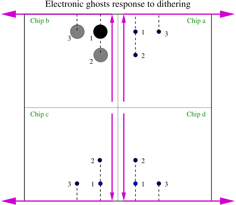
Figure 5: The electronic ghosts will move with or opposite to objects on the sky depending on the direction of sky motion relative to the direction of CCD readout (indicated by arrows for each quadrant). In the example shown here, the electronic ghost moves with the sky field on Chip a between dither positions 1 and 2, and on Chip c between dither positions 1 and 3.

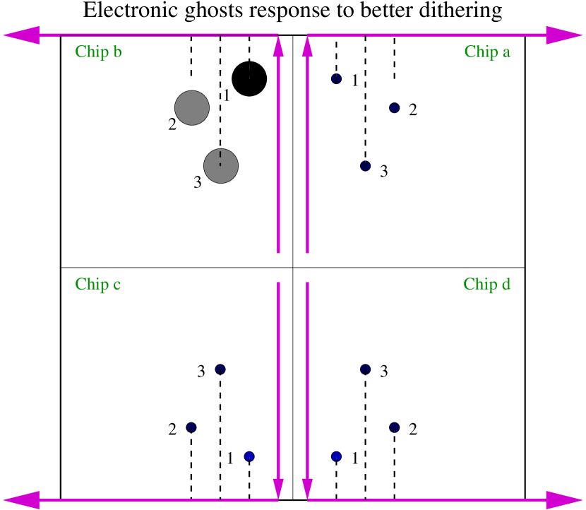
Figure 6: A new dither pattern that results in no ghosts being in the same position in the different images.

Chapter 12 Compressed FITS Performance Benchmarking for SNfactory

Appendix 12.A Summary

An investigation was performed to determine whether the FITS files should be processed compressed or uncompressed in the SNfactory pipeline. It was found that using compressed FITS files was in fact slower than using non-compressed FITS files with the Deeplib software used by the SNfactory.

Briefly, this resulted because the search pipeline was not actually I/O limited for the individual image manipulation operations. There was a timing log as part of the processing steps that would allow for a more precise analysis to try to reduce image processing time. It is possible that the way the Deeplib software manipulates files (by using pixel streams) is not optimal when dealing with compressed files, but this is the unlike to be the central issue with using compressed versus uncompressed FITS file.

The results of this study resulted in a decision to use uncompressed rather that compressed FITS files for the search pipeline image processing.

Appendix 12.B Timing Tests

After a few simple tests, the initial assumption that operating on compressed files would be faster given that the search pipeline would be be I/O bound appears not to hold:

pdsflx004 81% time sky ‘findimage feb112002oschinab84551.fts‘Image sigma: 20.24571.150u 0.350s 0:02.14 70.0%     0+0k 0+0io 923pf+0w

This file had not been accessed recently and there was no reason it should be in the NFS or disk cache of the computer or diskvault. The 1.150u refers to 1.15 user CPU seconds, while the 0.350s refers to the 0.35 seconds of system time, the 0:02.14 indicates total wallclock time, and the 70.0% is the CPU percentage.

A sample subtraction with the QUESTII camera in point-and-track mode took 9 minutes, 30 seconds with a CPU percentage of 43.8%. This was from a combination of I/O and database access times:

pdsflx006 15% time idl ‘whichdir 20030926 neat‘\/subdir/idlsubsep262003palomaag101307_360_240_6_i_aux198.630u 51.750s 9:31.40 43.8%  0+0k 0+0io 716764pf+0w

A time command was added to the processing of images to get up-to-date statistics on the processing of the images. Testing indicated that the compression imposes a significant penalty:

pdsflx004 157% time imarith sep22003questaaa32.fts.gz x sep22003questdaa75.fts.gz \   test2.fts.gzmode : wb5.150u 0.590s 0:06.12 93.7%     0+0k 0+0io 626pf+0wpdsflx004 158% time imarith sep22003questaaa32.fts.gz x sep22003questdaa75.fts.gz \   test2.fts.gzmode : wb5.010u 0.720s 0:07.68 74.6%     0+0k 0+0io 626pf+0wpdsflx004 159% time imarith sep22003questaaa32.fts.gz x sep22003questdaa75.fts.gz \   test2.fts.gzmode : wb5.410u 0.790s 0:06.80 91.1%     0+0k 0+0io 626pf+0wpdsflx004 160% time imarith sep52003questaaa96.fts x sep52003questaaa59.fts \   test.ftsmode : wb01.950u 0.440s 0:03.79 63.0%     0+0k 0+0io 625pf+0wpdsflx004 161% time imarith sep52003questaaa96.fts x sep52003questaaa59.fts \   test.ftsmode : wb01.950u 0.350s 0:02.59 88.8%     0+0k 0+0io 625pf+0wpdsflx004 162% time imarith sep52003questaaa96.fts x sep52003questaaa59.fts \   test.ftsmode : wb02.000u 0.300s 0:02.39 96.2%     0+0k 0+0io 625pf+0wpdsflx004 166% time imarith sep22003questaaa32.fts.gz x sep22003questdaa75.fts.gz \   test2.ftsmode : wb03.600u 0.290s 0:04.04 96.2%     0+0k 0+0io 626pf+0wpdsflx004 167% time imarith sep22003questaaa32.fts.gz x sep22003questdaa75.fts.gz \   test2.ftsmode : wb03.550u 0.250s 0:03.86 98.4%     0+0k 0+0io 626pf+0wpdsflx004 168% time imarith sep22003questaaa32.fts.gz x sep22003questdaa75.fts.gz \   test2.ftsmode : wb03.560u 0.370s 0:04.02 97.7%     0+0k 0+0io 626pf+0wpdsflx004 169% time imarith sep52003questaaa96.fts x sep52003questaaa59.fts \   test.fts.gzmode : wb3.120u 0.430s 0:03.60 98.6%     0+0k 0+0io 625pf+0wpdsflx004 170% time imarith sep52003questaaa96.fts x sep52003questaaa59.fts \   test.fts.gzmode : wb3.170u 0.340s 0:03.54 99.1%     0+0k 0+0io 625pf+0wpdsflx004 171% time imarith sep52003questaaa96.fts x sep52003questaaa59.fts \   test.fts.gzmode : wb3.120u 0.280s 0:03.49 97.4%     0+0k 0+0io 625pf+0w

The first three tests were from compressed input to compressed output files. The second three tests were from non-compressed input to non-compressed output files. The third three tests were from compressed input to non-compressed output files. The fourth three tests were from non-compressed input to compressed output files.

The fastest image arithmetic tests were the non-compressed to non-compressed runs, with an average of $2.9$ seconds total elapsed time. The slowest were the compressed to compressed runs, with an average of $7.2$ seconds. The mixed runs were in between these two extremes with an average of $4.0$ seconds for the compressed to non-compressed run and $3.5$ seconds for the non-compressed to compressed run.

As doubling the available disk space for the SNfactory was far cheaper than doubling our available processors, it was clear that using non-compressed files was the better approach.

References

- Alard (2000) Alard, C. 2000, A&AS, 144, 363
- Alard & Lupton (1998) Alard, C. & Lupton, R. H. 1998, ApJ, 503, 325
- Aldering et al. (2002a) Aldering, G., Adam, G., Antilogus, P., Astier, P., Bacon, R., Bongard, S., Bonnaud, C., Copin, Y., Hardin, D., Henault, F., Howell, D. A., Lemonnier, J., Levy, J., Loken, S. C., Nugent, P. E., Pain, R., Pecontal, A., Pecontal, E., Perlmutter, S., Quimby, R. M., Schahmaneche, K., Smadja, G., & Wood-Vasey, W. M. 2002a, in Survey and Other Telescope Technologies and Discoveries. Edited by Tyson, J. Anthony; Wolff, Sidney. Proceedings of the SPIE, Volume 4836, pp. 61-72 (2002)., 61–72 [ADS]
- Aldering et al. (2002b) Aldering, G., Akerlof, C. W., Amanullah, R., Astier, P., Barrelet, E., Bebek, C., Bergstrom, L., Bercovitz, J., Bernstein, G. M., Bester, M., Bonissent, A., Bower, C., Carithers, W. C., Commins, E. D., Day, C., Deustua, S. E., DiGennaro, R. S., Ealet, A., Ellis, R. S., Eriksson, M., Fruchter, A., Genat, J., Goldhaber, G., Goobar, A., Groom, D. E., Harris, S. E., Harvey, P. R., Heetderks, H. D., Holland, S. E., Huterer, D., Karcher, A., Kim, A. G., Kolbe, W. F., Krieger, B., Lafever, R., Lamoreux, J. C., Lampton, M. L., Levi, M. E., Levin, D. S., Linder, E. V., Loken, S. C., Malina, R., Massey, R., McKay, T., McKee, S. P., Miquel, R., Moertsell, E., Mostek, N., Mufson, S., Musser, J. A., Nugent, P. E., Oluseyi, H. M., Pain, R., Palaio, N. P., Pankow, D. H., Perlmutter, S., Pratt, R., Prieto, E., Refregier, A., Rhodes, J., Robinson, K. E., Roe, N., Sholl, M., Schubnell, M. S., Smadja, G., Smoot, G. F., Spadafora, A., Tarle, G., Tomasch, A. D., von der Lippe, H., Vincent, D., Walder, J.-P., & Wang, G. 2002b, in Future Research Direction and Visions for Astronomy. Edited by Dressler, Alan M. Proceedings of the SPIE, Volume 4835, pp. 146-157 (2002)., 146–157 [ADS]
- Aldering et al. (2004) Aldering, S. C. G., Althouse, W., Amanullah, R., Annis, J., Astier, P., Baltay, C., Barrelet, E., Basa, S., Bebek, C., Bergstrom, L., Bernstein, G., Bester, M., Bigelow, B., Blandford, R., Bohlin, R., Bonissent, A., Bower, C., Brown, M., Campbell, M., Carithers, W., Commins, E., Craig, W., Day, C., DeJongh, F., Deustua, S., Diehl, T., Dodelson, S., Ealet, A., Ellis, R., Emmet, W., Fouchez, D., Frieman, J., Fruchter, A., Gerdes, D., Gladney, L., Goldhaber, G., Goobar, A., Groom, D., Heetderks, H., Hoff, M., Holland, S., Huffer, M., Hui, L., Huterer, D., Jain, B., Jelinsky, P., Karcher, A., Kent, S., Kahn, S., Kim, A., Kolbe, W., Krieger, B., Kushner, G., Kuznetsova, N., Lafever, R., Lamoureux, J., Lampton, M., Fevre, O. L., Levi, M., Limon, P., Lin, H., Linder, E., Loken, S., Lorenzon, W., Malina, R., Marriner, J., Marshall, P., Massey, R., Mazure, A., McKay, T., McKee, S., Miquel, R., Morgan, N., Mortsell, E., Mostek, N., Mufson, S., Musser, J., Nugent, P., Oluseyi, H., Pain, R., Palaio, N., Pankow, D., Peoples, J., Perlmutter, S., Prieto, E., Rabinowitz, D., Refregier, A., Rhodes, J., Roe, N., Rusin, D., Scarpine, V., Schubnell, M., Sholl, M., Smadja, G., Smith, R. M., Smoot, G., Snyder, J., Spadafora, A., Stebbins, A., Stoughton, C., Szymkowiak, A., Tarle, G., Taylor, K., Tilquin, A., Tomasch, A., Tucker, D., Vincent, D., von der Lippe, H., Walder, J., Wang, G., & Wester, W. 2004, ArXiv Astrophysics e-prints
- Allen et al. (2002) Allen, S. W., Schmidt, R. W., & Fabian, A. C. 2002, MNRAS, 334, L11 [ADS]
- Antonucci (1993) Antonucci, R. 1993, ARA&A, 31, 473 [ADS]
- Bahcall et al. (2003) Bahcall, N. A., Dong, F., Bode, P., Kim, R., Annis, J., McKay, T. A., Hansen, S., Schroeder, J., Gunn, J., Ostriker, J. P., Postman, M., Nichol, R. C., Miller, C., Goto, T., Brinkmann, J., Knapp, G. R., Lamb, D. O., Schneider, D. P., Vogeley, M. S., & York, D. G. 2003, ApJ, 585, 182 [ADS]
- Bennett et al. (2003) Bennett, C. L., Halpern, M., Hinshaw, G., Jarosik, N., Kogut, A., Limon, M., Meyer, S. S., Page, L., Spergel, D. N., Tucker, G. S., Wollack, E., Wright, E. L., Barnes, C., Greason, M. R., Hill, R. S., Komatsu, E., Nolta, M. R., Odegard, N., Peiris, H. V., Verde, L., & Weiland, J. L. 2003, ApJS, 148, 1 [ADS]
-
Bes Optics (2003)
Bes Optics. 2003, Schott Optical Filters,
http://www.besoptics.com/html/body_schott_rg610_filter_glass.html [LINK] - Blanc (2002) Blanc, G. 2002, Master’s thesis, Saclay
- Blanc et al. (2004) Blanc, G., Afonso, C., Alard, C., Albert, J. N., Aldering, G., Amadon, A., Andersen, J., Ansari, R., Aubourg, E., Balland, C., Bareyre, P., Beaulieu, J. P., Charlot, X., Conley, A., Coutures, C., Dahlen, T., Derue, F., Fan, X., Ferlet, R., Folatelli, G., Fouque, P., Garavini, G., Glicenstein, J. F., Goldman, B., Goobar, A., Gould, A., Graff, D., Gros, M., Haissinski, J., Hamadache, C., Hardin, D., Hook, I. M., deKat, J., Kent, S., Kim, A., Lasserre, T., LeGuillou, L., Lesquoy, E., Loup, C., Magneville, C., Marquette, J. B., Maurice, E., Maury, A., Milsztajn, A., Moniez, M., Mouchet, M., Newberg, H., Nobili, S., Palanque-Delabrouille, N., Perdereau, O., Prevot, L., Rahal, Y. R., Regnault, N., Rich, J., Ruiz-Lapuente, P., Spiro, M., Tisserand, P., Vidal-Madjar, A., Vigroux, L., Walton, N. A., & Zylberajch, S. 2004, ArXiv Astrophysics e-prints
- Blanton et al. (2003a) Blanton, M. R., Hogg, D. W., Bahcall, N. A., Baldry, I. K., Brinkmann, J., Csabai, I., Eisenstein, D., Fukugita, M., Gunn, J. E., Ivezić, Ž., Lamb, D. Q., Lupton, R. H., Loveday, J., Munn, J. A., Nichol, R. C., Okamura, S., Schlegel, D. J., Shimasaku, K., Strauss, M. A., Vogeley, M. S., & Weinberg, D. H. 2003a, ApJ, 594, 186 [ADS]
- Blanton et al. (2003b) Blanton, M. R., Hogg, D. W., Bahcall, N. A., Brinkmann, J., Britton, M., Connolly, A. J., Csabai, I., Fukugita, M., Loveday, J., Meiksin, A., Munn, J. A., Nichol, R. C., Okamura, S., Quinn, T., Schneider, D. P., Shimasaku, K., Strauss, M. A., Tegmark, M., Vogeley, M. S., & Weinberg, D. H. 2003b, ApJ, 592, 819 [ADS]
- Branch et al. (1995) Branch, D., Livio, M., Yungelson, L. R., Boffi, F. R., & Baron, E. 1995, PASP, 107, 1019 [ADS]
- Branch & Miller (1993) Branch, D. & Miller, D. L. 1993, ApJ, 405, L5
- Branch & Tammann (1992) Branch, D. & Tammann, G. A. 1992, ARA&A, 30, 359
- Braun (2003) Braun, H.-W. 2003, High Performance Wireless Research and Education Network, http://hpwren.ucsd.edu/ [LINK]
- Burbidge (1967) Burbidge, E. M. 1967, ARA&A, 5, 399 [ADS]
- Cappellaro et al. (1999a) Cappellaro, E., Evans, R., & Turatto, M. 1999a, A&A, 351, 459 [ADS]
- Cappellaro & Turatto (1988) Cappellaro, E. & Turatto, M. 1988, A&A, 190, 10 [ADS]
- Cappellaro et al. (1999b) Cappellaro, E., Turatto, M., & Mazzali, P. 1999b, IAU Circ., 7091, 1 [ADS]
- Cappellaro et al. (1997) Cappellaro, E., Turatto, M., Tsvetkov, D. Y., Bartunov, O. S., Pollas, C., Evans, R., & Hamuy, M. 1997, A&A, 322, 431 [ADS]
- Cardelli et al. (1989) Cardelli, J. A., Clayton, G. C., & Mathis, J. S. 1989, ApJ, 345, 245