The XO Project: Searching for Transiting Extra-solar Planet Candidates

Abstract

The XO project’s first objective is to find hot Jupiters transiting bright stars, i.e. V $<~{}12$, by precision differential photometry. Two XO cameras have been operating since September 2003 on the 10,000-foot Haleakala summit on Maui. Each XO camera consists of a 200-mm f/1.8 lens coupled to a 1024x1024 pixel, thinned CCD operated by drift scanning. In its first year of routine operation, XO has observed 6.6% of the sky, within six 7°-wide strips scanned from 0° to $+63$° of declination and centered at RA=0, 4, 8, 12, 16, and 20 hours. Autonomously operating, XO records 1 billion pixels per clear night, calibrates them photometrically and astrometrically, performs aperture photometry, archives the pixel data and transmits the photometric data to STScI for further analysis. From the first year of operation, the resulting database consists of photometry of $\sim$100,000 stars at more than 1000 epochs per star with differential photometric precision better than 1% per epoch. Analysis of the light curves of those stars produces transiting-planet candidates requiring detailed follow up, described elsewhere, culminating in spectroscopy to measure radial-velocity variation in order to differentiate genuine planets from the more numerous impostors, primarily eclipsing binary and multiple stars.

1 Introduction

Borucki & Summers (1984) proposed detection of planets with the transit technique. At the time, their proposal was thought to be impractical because astronomers expected planetary systems to be like our own. In particular the Jovian-sized planets that could create a readily-detectable photometric transit would occupy orbits many AU in radius with periods of many years. Since the discovery of the “hot Jupiter” orbiting 51 Peg with a 4.23 day orbit, many attempts have been made to find hot Jupiters that transit stars bright enough ($m_{V}\lesssim 12$) for detailed studies to be performed with existing telescopes such as HST, Keck and the VLT (e.g. Vulcan, Stare, etc). The first such success was Tres-1 (Alonso et al. 2004). The OGLE collaboration’s successes were with fainter stars (Udalski et al. 2003).

The radius of solar-composition objects is expected to change by less than a factor of two (e.g. Burrows et al. 2001) over the entire range in mass from the bottom of the main sequence to less than a Jupiter mass. So transit observations by themselves provide no information about the mass of the planet (or brown dwarf, or red dwarf). On the other hand, radial velocity studies yield only minimum masses. However, the combination of the Doppler orbit and the observation of transits yields the gross physical characteristics of the planet: mass, radius, density, and “surface” gravity. A transiting planet is interesting in at least two other ways: 1) absorption of starlight is a much larger signal than reflected starlight, so for example absorption spectroscopy has already permitted detection of an exoplanet’s atmosphere (Charbonneau et al. 2002), and 2) the rapid and precisely predictable on/off nature of the transit permits excellent calibration, which among other things, allows one to search for natural satellites and Saturn-like rings orbiting the transiting planet and to attempt to measure the planet’s albedo by observing the reflected light of the planet being blocked by the star (Brown et al. 2001).

This paper describes the XO project’s design, implementation, and verification. Not an acronym but a name, XO is pronounced as it is in “exoplanet.” We describe the XO design requirements in Sec. 2, the hardware in Section 3, the observing strategy in Section 4, and the software in Section 5. Section 6 shows that our system is finding transiting hot Jupiter (THJ) candidates. In future papers we describe additional observations that test whether a candidate is definitely an impostor such as an eclipsing binary star, or potentially one of the THJs that we seek (McCullough et al. 2005).

2 Requirements

Pepper et al. (2003) formalize the optimization of systems designed to find THJs and have selected a 2-inch diameter telescope with a 4kx4k sensor as best for a $2\pi$ steradian survey of stars with V$\lesssim 10$. Independently we designed the XO system with a similar but simpler analysis for a limiting magnitude of V$\lesssim 12$, requiring a larger diameter aperture, d $\approx 0.1$ m, and in order to accommodate drift scanning, a smaller instantaneous field of view, 7°$\times$7°.

The XO system was designed to find THJs around stars bright enough to permit significant follow up as described in the introduction, i.e. ($m_{V}\lesssim 12$). The number of THJ-systems on the sky is estimated below from the number density of stars as a function of their brightness, the frequency of hot Jupiters around those stars, and the geometric probability of the orbit being inclined such that a transit can occur as seen from Earth. The photometric precision required is set by the fraction of the star’s area obscured by the THJ, $\sim 0.01$. The cadence of the observations is set by the need to have multiple observations made during the duration of the transit, $\sim 0.1$ day. The duration of an observing sequence is set by the need to observe multiple transits to define a tentative ephemeris. Given that useful observations are obtained only at moderate zenith angles during clear nights, the observing sequence must be much longer than the orbital period in order to witness at least 3 transits (Brown 2003).

Of stars brighter than $\rm m_{V}=12$ at the north galactic pole (NGP), there are 2.9 main sequence stars per $\Box^{\circ}$ with $\rm M_{V}=$ 4.5 to 5.5, and 1.3 with $\rm M_{V}=$ 5.5 to 6.5 (Bahcall & Soneira 1981). Solar-type and later stars with $\rm M_{V}>5$ and brighter than our limiting magnitude of $\rm m_{V}=12$ must be closer than $D=250$ pc, whereas for such stars the scale height $H=400$ pc. For a volume density of stars with exponential scale height H, the ratio of stars per square degree within a distance D at Galactic latitude $b=0$° to those at $b=90$° is $D/(H\times(1-exp(-D/H))$, which equals 1.34 for D/H = 250 pc / 400 pc = 0.625, and approximately equals 1 + 0.58*D/H for D/H $\leq 1$. The density enhancement in the galactic plane is countered by the disadvantages of crowding and confusion. For XO’s drift-scanned observations of a variety of Galactic latitudes, we empirically find the maximum surface density of stars with photometry sufficient for our purposes occurs at $b\approx\ 20$°(Section 6). Although stars become more concentrated toward the Galactic plane with earlier type, early-type stars are larger in physical size and thus are expected to have transits of lower amplitude that are more difficult to detect. For simplicity, we use the stellar density at the NGP in order to conservatively estimate that there are $\sim$160,000 solar type stars with $\rm m_{V}<12$ over the entire celestial sphere. The probability that a given solar type star has a THJ is 0.00075, because the fraction of stars with Jovian planets is 0.05 (Marcy & Butler 2000), the fraction of those planets with periods less than 7 days is 0.15 (Brown 2003), and the fraction of those that could exhibit transits seen from Earth is 0.10 (Borucki & Summers 1984). Thus, we expect 120 THJs orbiting solar type stars brighter than 12th magnitude, or 30 THJs orbiting stars brighter than 11th magnitude. The corresponding predictions are 7.5, 2, and 0.5 stars for $\rm m_{V}<10,~{}9,~{}and~{}8$, respectively.

There are at least three interesting points implied by the calculations above:

1. the 8th magnitude HD 209458 probably is the brightest star exhibiting hot-Jupiter transits,

2. there is likely one hot Jupiter transiting an 11th magnitude star for every 1400 $\Box^{\circ}$ of sky, and

3. at any given time approximately one bright ($\rm m_{V}<11$) star is being transited.

For simplicity, we have assumed the probabilities are independent and can be multiplied together. A thorough analysis of joint probability functions is beyond the scope of this paper, and indeed some of the joint probabilities are unknown (Brown 2003). Pepper et al. (2003) estimate there are $\sim$5 THJs orbiting stars brighter than V=10 mag for $\rm 4.5<M_{V}<5.5$, and scaling from their Figure 1 we estimate for V$<$10 an additional $\sim$6 THJs and $\sim$3 THJ for $\rm 3.5<M_{V}<4.5$ and $\rm 5.5<M_{V}<6.5$, respectively, if the frequency of THJs is independent of $\rm M_{V}$. We have based our requirements upon the statistics from radial velocity surveys, which are secure for solar type stars. However, if the estimate of Pepper et al. (2003) is appropriate, then we could hope for of order 200 THJs orbiting approximately solar sized (or smaller) stars brighter than 12th magnitude.

Succinctly, the XO system is required to image hundreds of square degrees of sky many times per hour for months, and from those images the software must enable photometry of stars $9\lesssim m_{V}\lesssim 12$ with a precision of $\sim 10$ millimag per measurement. Those requirements have been met by the XO Mark I system described below. Given the demonstrated performance of the Mark I system, we anticipate replicating it to speed the discovery of THJs.

3 Hardware Implementation

The XO Mark I hardware is described in this section. Figure 1 illustrates the cameras and equatorial mount; Figure 2 gives a block diagram of the system; and Table 1 summarizes the components.

Many systems have been built to discover THJs orbiting bright stars (Horne 2003). Some of the unique aspects of the XO system are that it uses a broad spectral bandpass (0.4 $\mu$m to 0.7 $\mu$m) to collect more photons per second, drift scanning to simplify calibration, aperture photometry for simplicity and reliability, and two identical cameras pointed in the same direction to collect more photons and to provide redundancy so that observing will not be entirely interrupted due to failure of a single camera or its control computer.

Sometimes a component is unresponsive and must be reset by cycling its AC power. We accomplish this either by human intervention either in person or remotely using a network power strip that permits remote control of 8 AC power outlets independently (Figure 2). The network power strip is one of the essential components in the XO system and it has operated 100% reliably.

Table 1: Summary of the XO Mark I Equipment

Location:
Haleakala, Maui	Longitude:	Latitude:	Elevation:
	$156^{\circ}$15’.3W	$20^{\circ}$42’.4N	3054 m
Shelter:
roll-off roof	Cable-	1/4 HP gear motor	Surveillance camera
	driven	Grainger Inc. 5K942	AXIS Inc. 2100
Mount:
Paramount ME	German-	Scan rate in RA:	Scan rate in Dec.:
Software Bisque Inc.	Equatorial	sidereal	478 arcsec$\cdot$sec-1
Objective:
Canon EF200 lenses (two)	Diameter:	Focal ratio:	Plate scale:
	0.11 m	f/1.8	1.058 ”/$\mu$m
Filter:
50 mm diameter, 3.3 mm thick	Bandpass:	Transmission:	${\lambda}_{cutoff}$:
Edmund Optics Inc. NT54-517	flat over	$\sim$ 95%	700 nm
	$400nm<\lambda<{\lambda}_{cutoff}$
Detector:
Apogee Ap8p CCD	1024 x 1024	FOV:	Pixel scale:
thinned	24$\mu$m pixels	$7^{\circ}.2\times 7^{\circ}.2$	25.4 “/pixel

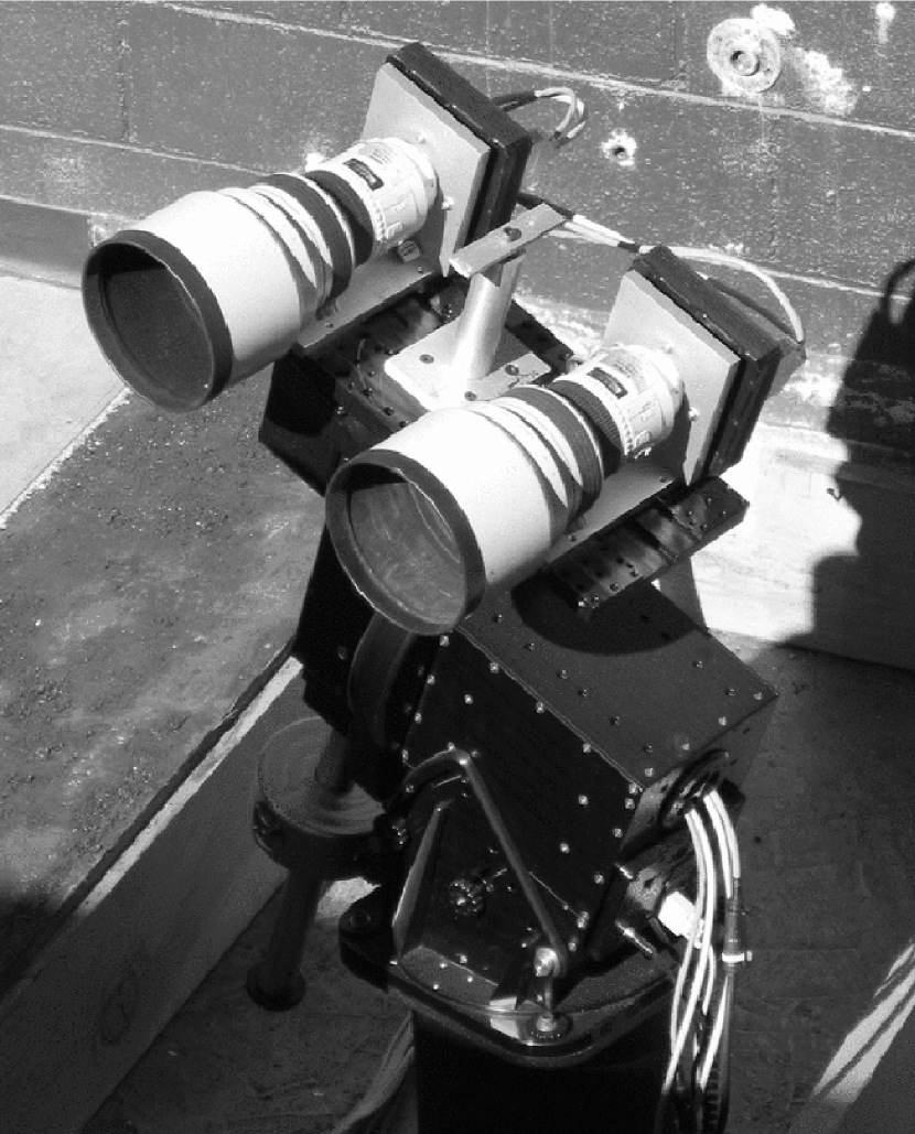
Figure 1: The XO Mark I observatory: two 200 mm f/1.8 lenses and 1K$\times$1K CCDs attached to a German equatorial mount, deployed under a roll-off roof.

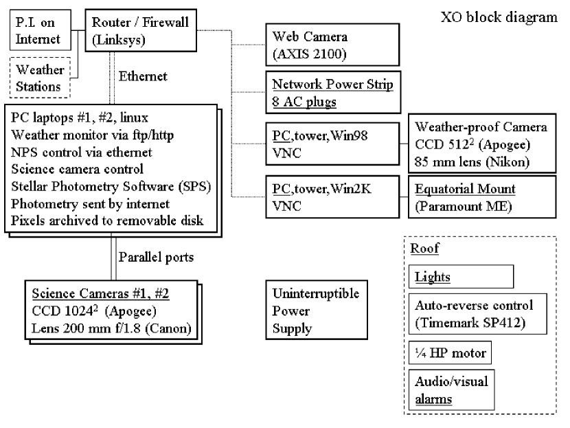
Figure 2: The XO Mark I system block diagram.

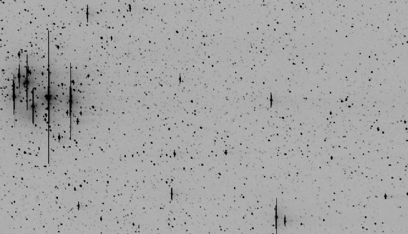
Figure 3: A representative section of a flat-fielded XO image shows the Pleiades star cluster (left side). This 1024-column section is as wide as the XO images, 7.2° but is only 6% of the 9000-row height of the scans. The vertical and horizontal trails from very saturated stars do not prevent good photometry of most of the stars in each image.

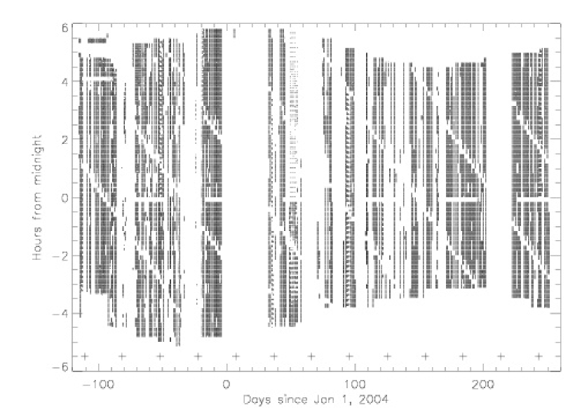
Figure 4: The periods of time spent observing during the first year of operation are plotted. The dates of full moon are indicated with plus signs.

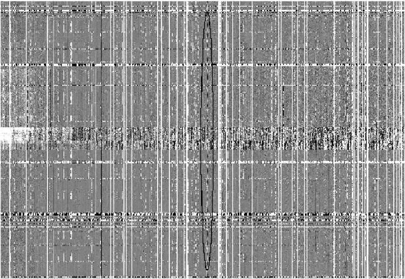
Figure 5: This figure shows a representative section of a calibrated array of differential stellar magnitudes, with each column corresponding to a single star, and each row to a single epoch. The mean magnitude of each star has been subtracted from each column. Bad data have not been flagged. Ideally the entire image would be white noise, less at the left (brighter stars) and more at the right (fainter stars). In practice data are missing (white) and trends are evident (see text). Visual inspection of diagrams like this reveals trends and assists in improving the calibration. Large amplitude variable stars are also apparent; an example near the middle of the figure is shown inside the ellipse.

3.1 Weather Sensing and Roof Control

Gaustad et al. (2001) enlisted a human operator of an adjacent facility to authorize or to override, via email, the nightly opening and closing of the dome protecting their robotic telescope. The XO system observes without human assistance. Weather hazardous to the equipment is sensed in near real time as described below, and weather that is not hazardous but is unsuitable for observing is sensed after the fact by the science data analysis software.

We use three sources of weather data to determine whether to open our roof. The first is a CCD camera to detect stars. The second source is a set of weather stations operated by other tenants on the mountain. The third is a forecasting service operated by yet another tenant. If all three services are operating, then the data from every one must meet specific criteria for our system to open its roof. If one of the second or third services is inoperable, we reconfigure our system to ignore it. These three sources of weather data are described in turn below.

A small camera mounted in a weather-proof enclosure is aimed near the north celestial pole. At regular intervals, the PC takes a short exposure of a $\sim 3$-degree field of view. If the sky is clear, many stars are visible in the image and our software can determine an astrometric solution in the same manner as it does for our science images (Section 5.2). However, with time the images became increasingly defocused, due to wind shaking loose the lens’ helical focus mechanism. To compensated for this issue remotely, we adopted a different and more robust algorithm that works well with even very defocused images. The algorithm operates on two images taken twenty minutes apart. It rotates one image about the pole in order to register it to the other image, and if the two-dimensional cross-correlation function peaks within $\pm$3 pixels of the center and is greater than an empirically-determined threshold (0.17), then we assume the sky is clear. The latter algorithm is simple and effective, so we have not returned to the original algorithm of matching patterns of stars, even after re-adjusting the focus. We note that pointing the camera near the pole has some advantages: 1) sunlight cannot reach the lens and thereby damage a shutter, 2) rain (or snow) slides off the inclined window, and 3) clouds tend to come from up from below on Haleakala, so we think aiming our weather camera at a large zenith angle gives early warning of fog rising up the mountain.

If the data from any of the weather stations triggers any of the following conditions, then we close the roof, or keep it closed: 1) data are non-existent or stale, i.e. older than 30 minutes, 2) humidity $>$ 75% or dew point $<4$° C from ambient, 3) temperature $<-5$° C, 4) wind velocity $>20$ m s^-1, 5) non-zero rain accumulation in the past 10 minutes, 6) sunlight detected on a solar cell. Humidity and/or dew point accounts for nearly all closures. Because the humidity on Haleakala tends to be quite bimodal, either very low or nearly 100%, and because high humidity should correlate with poor photometric precision, we have not attempted to optimize the thresholds for humidity and dew point.

Another tenant on Haleakala operates weather sensors and a neural network prediction of the probability of inclement weather in the near future (a “forecast”) and now (a “nowcast”). XO closes its roof if the “forecast” or “nowcast” indicates a 95% or greater probability of inclement weather.

3.2 Drift Scanning

Drift scanning is efficient if the number of rows readout is much larger than the number of columns, i.e. for long, rectangular fields of view. Its advantage over staring-mode imaging is that the flat-field and the dark correction are homogenized by shifting the charge through all the rows. Thus, the drift-scanned vectors are more uniform and smoother than their staring-mode counter parts, which are 2-D arrays. The drift-scanned PSF is slightly wider in both directions compared to what it would be with “standard” staring-mode observations, but this is beneficial in the following sense. Drift scanning makes intra-pixel gain variations irrelevant; even intra-column variations are homogenized due to the fact that stars do not track perfectly parallel to columns. The drift-scanned PSF is approximately a Gaussian with FWHM = 1.8 pixels. During the first year of operation, the correlation coefficient of the observed PSF with a FWHM=1.8 pixel Gaussian is $\sim 0.80$ with no measurable dependence on time of night, day of year, hour angle, or temperature from 3° C to 16° C. The correlation coefficient is expected to be variable with position on the CCD, because the scan rate cannot be optimum for all columns of the CCD. Indeed if the scanning of the CCD and mount are purposefully not synchronized, for example in order to mitigate saturation of very bright stars by elongating them, the PSF elongates in the center of the CCD and becomes shaped like a “)” or a “(” on either side of center. With proper synchronization, the elongation is nearly imperceptible and nearly uniform across the field as intended (see Figure 6).

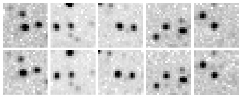
Figure 6: Images of stars are nearly uniform across the field of view. Subimages centered at CCD columns 100, 300, 500, 700, and 900 (left to right) are displayed for camera 0 (top) and camera 1 (bottom). The two cameras observe nearly the same field of view simultaneously; in their native format, they are misaligned by 13 columns, i.e. 1.3% of the sensor’s width, but we have shifted one by 13.0 columns for this plot.

By rotating the mount at 478″ s^-1about the declination axis while tracking at the sidereal rate in right ascension, the XO system scans repeatedly from 0° to 63° of declination.

The repeatability of a star’s position in rows, Y, is directly related to the repeatability of the timing of the CCD readout and its synchronization with the equatorial mount. Typically the repeatability is $\pm$1 second, corresponding $\pm$19 rows, peak to valley. Occasionally larger excursions occur, e.g. due to missing the daily reset of one of the computers’ clocks. The clocks on the computers reading the CCDs drift reliably by 4 seconds per day.

The repeatability of a star’s position in columns, X, is directly related to the repeatability of the mount’s positioning in RA. The repeatability measured over an observing season is $\pm 4$ columns ($\pm 100$″), peak to valley, dominated by a slowly-varying function of hour angle presumably due to residual misalignments or imperfections in the mount.

We constructed a “flat field” vector from a robust averaging of measurements of “sky” along columns of a few images selected to be relatively free of stars, saturated stars, Galactic cirrus, and gradients or curvature. The “flat field” for each camera is approximately parabolic, with the peak within 6 columns of the center of the CCD, and it is almost entirely due to optical vignetting, because the detectors are intrinsically uniform and are made even more so by the drift scanning technique. At the edges, a noticeable departure upward occurs that we attribute to excess scattered light from the sky near the edges of the CCD. We replaced the edges of the measured “flat field” vector with linear extrapolations from the interior. Other than a bad column in each of the CCDs, we did not measure any repeatable, small-scale structure in the observed flat field vector, so we smoothed it with a 31-column boxcar. The flat field’s peak, near the center column of the CCD, is greater than its minimum at one of the edges, by 34% and 35% respectively for the two cameras. The absolute value of the slope of the flat field is everywhere $<0.9$ millimag column^-1. The slope combined with the repeatability in X-position implies repeatability of the instrument of $\pm 3.6$ millimag, peak to valley, prior to calibration.

3.3 Mount Control

The equatorial mount selected is a Paramount ME manufactured by Software Bisque, Inc. We control the Paramount using a custom visual basic script interacting with The Sky by the same manufacturer. The script commands the mount to scan every ten minutes according to a pre-determined nightly schedule. For simplicity, the script and the mount operate regardless of the roof’s state.

The Paramount has required no physical maintenance, and we have experienced only a few minor problems with it. The cameras are re-oriented by 180° on the sky whenever the German equatorial mount crosses the meridian. This requires scanning northward east of the meridian and southward west of the meridian; it also requires calibrating the data separately, because the positions of a given star on the CCD are not the same on opposite sides of the meridian.

3.4 Charge Coupled Devices

The sensors selected are SITe SI-003AB 1024²-pixel back-illuminated CCDs with 24 micron pixels, in the model AP8p camera manufactured by Apogee, Inc. The CCD is cooled thermoelectrically, with waste heat dissipated by fans on a heat sink. Because the CCD is illuminated by a broad optical bandpass with a f/1.8 lens, dark current can be nearly negligible with moderate cooling, so for simplicity and reliability, we operate the CCDs in MPP mode at $-30$ C year round. A disadvantage of the MPP mode for these sensors is that in addition to “bleeding” vertically, bright stars leave trails horizontally. In order to eliminate the horizontal trails, MPP mode can be suppressed during readout. However that option is not suitable for drift scanning wherein the CCD is read continuously. Operating the CCD without MMP mode increases the dark current by a factor of 20, which we decided would be less desirable than having trails associated with a few very bright stars per image. Each CCD has one unique bad column, but for surveys such as this, sensors with a single bad column can be more cost effective than ones with no bad columns. We flag data for which a star’s photometric aperture contains a bad column.

4 Observing Strategy and Experience

Our observing strategy is based upon a compromise between observing a region of sky for many weeks and observing at moderate zenith angles. As stated before, we scan in declination from 0° to +63°, and each night a program selects the right ascensions $\alpha$ of the scans from a table. Each star is observed by each of the two cameras every 10 minutes. On a given night, we either concentrate on a particular RA, $\alpha_{0}$, or split the night at midnight and observe one RA, $\alpha_{-}$, before midnight and another RA, $\alpha_{+}$, after midnight. In the former case, we observe the primary target whenever its hour angle is within 4 hours of the meridian, and after/before it is within that range we observe RA=$\alpha_{0}\pm 4$ hours. With this strategy, a season of observing a given target lasts $\sim$4 months, as follows: it is observed only a few times in the morning for the first $\sim$0.5 month; from midnight to morning for the next month; whenever it is within 4 hours of the meridian for a month; from evening until midnight for a month; and finally only a few times in the evening for the last $\sim$0.5 month of its season. In a calendar year, this strategy targets six RAs, each separated by 4 hours from its neighbors. The visibility function as a function of period of the transits for a representative star is given in Figure 7. A second season of observation of the same stars improves the visibility of transits, especially for longer orbital periods, but at the cost of not observing “new” stars. With a second observing season on the same stars, the longer time baseline permits more precise period determination, which is important for predictions of future transits and for accurately estimating the orbital phase of radial velocities.

Figure 7: The visibility of transits of a given period are indicated for observations of at least 1 transit (solid), at least 2 transits (dotted), and at least 3 transits (dashed). In the plot, the fraction of transits seen indicates the fraction that could be seen with sufficient detection sensitivity, given the actual times of observation of RA=0^h by XO in 2003. Characteristically, the visibility is excellent at periods of 3 days or less and tapers off rapidly for longer periods.

XO’s 25″ pixel^-1 scale is approximately twice that of other similar projects (Figure 3). This is primarily because our system was designed to scan large regions of sky, typically far from the Galactic plane, where the stellar density per unit solid angle is small. Also, the greater surface brightness in the Galactic plane elevates the photometric noise. As stated earlier, XO’s targets are approximately isotropically distributed on the sky. Therefore, at low Galactic latitudes we expect that the number of solar type stars to be enhanced somewhat but the number of false positives to be enhanced greatly, either astrophysically (Brown 2003) or instrumentally, i.e. that the crowding will make the photometry more error prone.

In the first year, the XO system’s operational readiness was as follows: 1) it missed 36 contiguous nights (10%) due to a roof motor failure caused by warping of the roof’s rails at the onset of winter, 2) it did not observe 22 additional nights (6%) due to various shorter-term equipment or software problems throughout the year, 3) it did not observe at all on 62 nights (17%) due to weather, and 4) of the remaining 245 nights (67%), data was gathered for some fraction of the night, with that fraction being distributed on [0,1] approximately uniformly.

Figure 4 shows many patterns to the actual observations in the first year. The hour-glass shape is due to the annual pattern of times of darkness for Maui. The sky is more often cloudy in summer than winter. The roof was inoperable for all of January 2004. The telescope stops observing for 10-30 minutes when transitioning from one target RA to another (which often occurs near midnight) and at meridian crossing (ragged slanted lines). Moon light saturates the detector when the telescope scans near the moon, so some data is lost around full moon; for example, on nights 94-96 moonlight saturated the southern part of each scan. The ragged data after midnight on nights 50-55 was caused by a software error: we had been discarding any image with fewer than 5000 stars detected, but for RA = 12 hours, this threshold was too high, so we adjusted it to be 1500 stars. Our linux operating system performed housekeeping by default at 4 AM, and until we forced this to occur during daytime, images at 4 AM were discarded because they were trailed slightly (nights -112 to -89). During approximately that same period, we had a simplistic schedule of observing only RA = 0 hours, and we kept the shutter-closed images taken during twilight.

5 Software Implementation

5.1 Readout of CCD

We accomplish the CCD readout in drift-scan mode using Tcl scripts and linux drivers for the Apogee cameras. We modified the Random Factory Version 0.5 GUI interface to permit command-line control, because the latter is better suited to autonomous operation. We used Xvfb to create a virtual frame buffer to work around the code’s default operation within X windows.

Each CCD is attached to a laptop computer’s parallel port for control and data transfer. The laptop operates the CCD on a predetermined schedule, initiated by linux’s cron every 10 minutes. During twilight the camera’s shutters are not opened but the CCD is readout just as it will be during normal (shutter-open) operation. Whenever the sun’s altitude $<-15$°, the control computer checks the weather (Section 3.1) and if it is clear, it opens the roof and the camera’s shutter and reads the CCD at a rate of 18.8 rows per second. The first 1024 rows are discarded because they are improperly exposed, and the next 9000 rows are stored as a FITS file. These files are automatically analyzed the following morning as described in the next Section.

Rarely, one of the linux laptops “freezes” and must be revived by human intervention. On the summit of Haleakala, the laptops are at their specified limit for ambient atmospheric pressure (altitude $<3048$ m), and for the first year they were routinely operated at too high an ambient temperature, especially for a few hours each morning when they reduced data. The frequency of “freezes” has been reduced to once every few months by increasing ventilation to reduce the temperature of the laptops’ ambient environment by $\sim$5 C to within specification (T $<31.3$° C).

Initially we operated the CCD’s only at night, warming them in the morning and cooling them at night. This was to reduce the risk of a power outage causing an uncontrolled return to ambient temperature that might crack the CCD or its thermoelectric cooler. However, occasionally a CCD would not cool after turning it on at nightfall, so we chose to leave them on and cooled all the time. XO has experienced at least one power outage that outlasted the UPS, but no equipment was damaged.

5.2 Data Reduction to Instrumental Magnitudes

Although the data are taken as 1024x9000 pixel arrays, for convenience we carve them into nine 1024x1024 images for further analysis. We carve the images at a 1000-row pitch, which allows for 24 pixels of overlap between images so that we do not loose stars due to the carving. During twilight we drift-scan images in the same manner as we do during the night except that we do not open the shutter. The last one exposed each night is used to create a “dark” vector to subtract from all the images taken during the night. We constructed a “flat field” vector as described in Section 3.

For each dark-subtracted and flat-fielded image, we use stars to determine the astrometric solution and add it to the header (Gaustad et al. 2001). Also we add keywords related to the weather and the positions of the Sun and Moon. Next, we use Stellar Photometry Software (SPS, Janes & Heasley 1993) to find stars by searching for peaks in the image’s cross correlation with a nominal Gaussian PSF. For each such star SPS measures the centroid in X and Y on the CCD, the instrumental magnitude using aperture photometry, the estimated error in that magnitude, the local sky level and the correlation coefficient of the star’s PSF with the Gaussian PSF used to find the stars.

A representative line of data stored for a given observation of one star is in fixed ASCII format, “1008.73 1001.02 12.7234 0.0028 2280.85” for the X, Y, Mag, Error, Sky+CC, respectively. The last quantity encodes the sum of the sky level rounded to the nearest integer and the correlation coefficient. Using this simple ASCII format, each star’s photometry requires 40 bytes uncompressed. Using standard gzip compression, the file compresses by a factor X, where X = 2.12+0.3log₁₀S, where S is the size of the ASCII file in kilobytes. For typical file sizes of 250 kB, the compression factor X = 2.8, so each star requires 14 bytes of information per camera per epoch.

Each day the previous night’s photometric measurements from SPS and the associated FITS headers for each image are transmitted to STScI for further calibration, which is described in the next section. All of the calibrated pixel data and the photometry of all of the stars detected in each image are stored on external disks that are mailed to STScI when they are filled, typically every 3 months. The conversion from raw to calibrated pixels is reversible to $\pm$1 ADU accuracy, so we discard the raw data and store the calibrated pixel data after applying lossless compression with “encode” (Sabbey 1999).

In the first year of operation, we gathered $\sim$132,000 1-Mpixel images that were of sufficient quality for our pipeline to recognize a star pattern. The data volume after lossless compression is 184 GB. During a clear, 10-hour, winter night the system gathers 1100 1-Mpixel images. Transmitting all the pixel data via the internet is possible but would use a significant fraction of the bandwidth from the summit, so the data-taking computers reduce the data from pixels to stellar photometry each morning and only transmit the photometry, which is 15 times fewer bytes than the pixels.

5.3 Data Organization and Visualization

The first part of the calibration pipeline arranges the SPS output from each image and its associated FITS header into an organized format. For each field we hand-pick a single image taken on a clear moonless night and extract a list of reference stars. The reference list defines the stars that we study for that field. Very many stars observed and analyzed with SPS are ignored by our pipeline because they are too faint to be on the list of reference stars. In our current implementation, we select stars with instrumental magnitude less than 16 (corresponding to V $<$ 13.3), and also we select only the brightest 5000 stars in each field.

The stellar photometry from each night is arranged into 2-D arrays stored as FITS files, with one axis indexing stars and the the other axis indexing epoch. Each photometric attribute that is appropriately stored for each star and epoch is stored as a separate FITS file. The attributes stored in this manner are X position, Y position, instrumental magnitude, predicted error in the magnitude, sky brightness, cross correlation coefficient, RA, DEC, and airmass. By ordering the stars according to their apparent magnitude, and ordering the epochs in time, we can conveniently see trends or errors in calibration by visualizing the photometry as an image (Figure 5).

An accompanying 2-D FITS file stores information associated with each image and epoch as a whole, extracted from the FITS header. Example keywords are those describing the astrometric solution, the Julian date, the weather (humidity, temperature, pressure, etc), the positions of the Sun and the Moon, a prediction of the sky’s surface brightness due to moonlight (Krisciunas & Schaefer 1991), etc. In total $\sim$60 such keywords exist for each image.

5.4 Calibration

The calibration is based upon these principles: 1) the drift-scan observing method inherently should provide repeatable and precise measurements, 2) only differential magnitudes are required, 3) at the amplitudes and on the timescales in which we are interested in, the majority of stars are constant in brightness and can be used as calibrators, and 4) each star will have its own unique set of comparison stars for differential, ensemble photometry.

The calibration is done iteratively. First we apply nominal calibrations to all stars, such as nominal airmass corrections, low-spatial-frequency corrections to the flat field, and offsets to bring the two cameras’ magnitudes into agreement. The sole purpose of this “zeroth order” calibration is to permit us to assign comparison stars that are nearest to the target star in brightness and in position, i.e. in columns of the CCD. The justification for this method is that stars of similar brightness that traverse the CCD at nearly the same location should make good comparison stars because uncorrected errors of calibration will be made equally to them all and will vanish in differential measurements. Because brightness and position cannot be directly compared, we determine the “nearest” stars by repeatedly bifurcating the sample of stars, first by distance in columns, then by difference in magnitude, and at each bifurcation, retaining the nearer half. We repeat the process as long as the sample exceeds 80 stars, from which we pick the 10 nearest to the target star’s magnitude as comparison stars.

Now that we have assigned comparison stars, we begin again the calibration starting with the raw instrumental magnitudes. Because each CCD has its own instrumental signature and because the CCD’s orientation on the sky changes by 180 degrees on opposite sides of the meridian due to the German equatorial mount, we perform the calibration for four cases distinctly: 1) CCD 0 scanning south, 2) CCD 1 scanning south, 3) CCD 0 scanning north, and 4) CCD 1 scanning north. Near the end of the calibration we combine the four cases. We apply a nominal correction of 0.086 magnitudes per airmass. Next, an empirically-determined third-order correction to the flat field is applied. Equivalently we could have adjusted the flat field vector itself, but that would necessitate re-processing all the pixels again, so it is more convenient to adjust the magnitudes. We subtract from each and every star’s light curve its average magnitude, so hereafter each star’s average magnitude is zero, facilitating comparisons. (Here and elsewhere, “average” refers to a resistant mean with outlier rejection.) At each epoch we subtract from the target star’s magnitude the average magnitude of its comparison stars for that epoch. We use a robust average as described previously, but a possible enhancement would be to use a weighted average as described by Kovács et al. (2005). Also for each epoch we use stars with ${\rm 10<V<11}$ to determine a third-order polynomial fit to the residual magnitudes with respect to the column on the CCD, and we subtract that fit from all the magnitudes at that epoch. For each star, we fit and subtract any linear dependence on airmass that remains; we presume this corrects for color differences between the target star and its comparison stars. For XO’s 0.4 $\mu$m to 0.7 $\mu$m bandpass, maximum zenith angle of $\sim$60 degrees, maximum angular separation between target star and reference star(s) of 7°, the expected residuals due to differential airmass between target and reference are small, $\lesssim 2$ millimag. Because we choose our reference stars so that they’ll have similar CCD columns, they tend to have similar right ascensions, and in our case that tends to make the differential zenith angle much smaller than the angular separation of the target from the reference(s) at large hour angles where the correction is most important. Figure 5 illustrates the data after calibration and before flagging.

We flag entire epochs for which the rms residuals of the stars with ${\rm 10<V<11}$ exceeds 12 millimag. We flag particular data points for which the SPS-estimated error exceeds 15 millimag, or for which the sky brightness exceeds 10000 ADU. The flagging eliminates most of the data for nights within a couple days of full moon, but after the period searching is finished (Section 5.5), these points can be re-examined by a human who can more effectively ignore the uncalibrated effects of the moonlight. We selected the red edge of our spectral bandpass (0.4 $\mu$m to 0.7 $\mu$m) in order to avoid the rapid increase of the brightness of the night sky in the near infrared and the telluric absorption bands therein. For a simple filter that transmits light shortward of a wavelength $W$ in microns, while holding all other characteristics of our system constant and optimizing for the spectrum of the night sky with no moonlight, we predict optimum sensitivity to V=12 solar-type stars with $W=0.77$, with values of $W$ between 0.7 and 0.85 giving signal to noise ratios within 10% of optimum. To reduce saturation from moonlight and to avoid potential variability of the telluric absorption bands, we selected $W=0.7\mu$m.

In Figure 5 data are missing due to clouds (horizontal lines), saturation (e.g. ragged left edge near center), a star positioned near a bad column in one CCD but not the other (vertical “dotted” line segments), or the star’s reference position being erroneous (vertical lines). Prior to calibration, trends are evident such as extinction varying with airmass (nightly undulations in the grey scale) or noise increasing with sky brightness (monthly cycle due to the moon). The effects of calibration and thresholds for flagging can be visualized with images of this type. For example, one can see that after our nominal calibration, the brightest stars (first $\sim$100 columns from the left) still have more noise than expected, because the grey scale is smoother for somewhat fainter stars (columns 100-300). Presumably the cause is that the peaks of the brighter stars saturate the CCD, especially when the moon elevates the sky level on the CCD.

5.5 Searching for Transit-like Light Curves

We use a modified form of the Box Least Squares (BLS) algorithm to search light curves for transit-like signatures (Kovács et al. 2002). The core of the algorithm is the FORTRAN subroutine “bls.f” modified by one of us (P. R. M.) to correct a small error in the original that did not treat transits near phase zero properly. Kovács renamed it “blsee.f,” tested it, found it to execute approximately as fast as the original, and distributes it on the internet alongside the original.

We call the BLS code from within IDL, thereby allowing the flexibility of IDL with the speed of FORTRAN. Because the execution time for the BLS routine is linear with the number of frequencies searched, and because generally we wish to measure only the peak(s) of the BLS spectrum, we have created an adaptive mesh search routine that first creates a nominal BLS spectrum using 5400 frequencies between 0.1 day^-1 and 0.95 day^-1, with spacing ${\Delta}f$ such that $f/{\Delta}f=2400$. We chose the frequency resolution $f/{\Delta}f=2400$ in order to resolve peaks in the BLS spectrum created by two dips in the light curve, each two-hours long, separated by 100 days, which is approximately the duration of an observing season for one field of view. The adaptive mesh searches near the 40 highest local maxima of the spectrum in order to quickly find the highest of those. While the 0.1 day^-1 may be justifiable based upon the diminishing sensitivity of our observing window to longer periods, the 0.95 day^-1 limit is a error of expediency that we intend to correct in future analyses by extending the search to frequencies greater than 1 day^-1 and using a notch filter to ingore frequencies very near 1.0 day^-1.

6 Verification

Figure 8 demonstrates that the XO system meets the photometric requirement described in Section 2. The most important component of noise is the Poisson noise due to the sky brightness integrated within a 3-pixel (76″) radius of the photometry aperture. The radius was selected as a compromise between smaller apertures optimized for fainter stars and larger apertures optimized for brighter stars. For simplicity we did not adjust the aperture according to the brightness of the star, and because the PSF is spatially dependent and occasionally can be slightly elongated due to imprecise scanning of the telescope mount, we selected the best single-radius compromise. For those same reasons we did not attempt to implement image-subtraction techniques (e.g. Alard 2000). For the XO observations, scintillation is expected to be $\lesssim 0.003$ mag (Dravins et al. 1998, Eq. 10). In Figure 8, the two slanted lines, derived from XO observations calibrated absolutely to LONEOS catalog stars (Skiff & Richmond 2003), cross at V=10.7, which is the magnitude of a star whose light equals that of the night sky in the r=76″aperture. This corresponds to a sky brightness of V=21.4 per $\Box^{\prime\prime}$, which equals the value independently measured for the dark sky near the zenith observed from 2800-m level on Mauna Kea at the same phase in the solar activity cycle (Krisciunas 1997). One penalty of the large photometric aperture is that during times of bright moonlight, the sky brightness can degrade the photometry considerably. For lunar phase within 30° (i.e. 2.5 days) of full, the moonlit sky is brighter than the dark sky by 2 mag or more (Krisciunas & Schaefer 1991) and the XO observations are not useful for planet transit observations, as can be appreciated by considering the effect of shifting the steeply-sloped line in Figure 8 to the left by 2 mag or more.

In Figure 8, the smallest values of $\sigma$ in the field are $\sim$0.0045 mag; the equivalent values for fields near the Galactic pole or plane are $\sim$30% lower or higher, respectively. Presumably stellar crowding is adversely affecting the aperture photometry, especially at low Galactic latitudes. The increased “sky” brightness due to the Galaxy increases $\sigma$ by as much as a factor of two from that plotted in Figure 8 for stars with $|b|\lesssim 10$ and V$>$11. The latter effect is offset by the variation of the number density of stars as with $|b|$ such the number of stars for which $\sigma<0.014$ mag peaks at $\sim$60 stars per $\Box^{\circ}$ at $|b|\approx 20$° and is $\sim$20 and $\sim$30 stars per $\Box^{\circ}$, respectively near the Galactic poles and plane. While those values are empirically determined for the XO system, the functional dependence of $\sigma$ on the dominant components of noise (see Figure 8) is sufficiently good that one could optimize a observing system for a given range of $|b|$. While XO was designed for moderate $|b|$, other systems have been optimized for $|b|\approx 0$° by using smaller pixels (in arcseconds) and demanding a sharper PSF and thereby allowing smaller synthetic apertures for their CCD photometry.

In Figure 8, the sparse envelope above the predicted noise curve includes stars with elevated noise, in addition to stars with instrinsic variability. Several factors cause the elevated noise, including bleeding of charge from bright stars, blending of stellar images, vignetting, etc. We have not yet thoroughly investigated all of these effects because even with the elevated noise, we have adequate sensitivity to detect planetary transits from a large sample of stars. Light curve analysis then eliminates candidates with sources of variability other than transits. Prompt THJ discovery is important, so that the Spitzer and Hubble Space Telescopes are still available for precise followup observations.

Figures 9, 10, and 11 show light curves for two of many XO transit candidates. The light curve in Figure 9 has the depth, but not the shape, expected of a THJ. Nonetheless, the figure demonstrates that the XO system has the sensitivity and sampling required to detect planetary transits. As XO’s temporal and angular coverage continues to increase, the odds of discovering one of the $\sim$8 THJ systems with $V\leq 10$ (Section 2) increases. A fundamental challenge is distinguishing actual planetary transits from a large number of false positives caused by a variety of non-planetary transits (e.g., Seager & G. Mallen-Ornélas 2003; Torres et al. 2004; 2005). The light curve shown in Figure 9 is more V-shaped than U-shaped, suggesting a grazing eclipse in a binary system or an eclipsing binary diluted by a third star. In fact, higher resolution images reveal a visual binary with a separation of $\sim 1$″, which is too small to induce a shift in the centroid measurable with XO as illustrated in Figure 12. McCullough et al. (2005) describe in detail our followup strategy and results for this and other transit candidates detected by XO.

The astrometric repeatability of well-exposed and reasonably isolated stars in the XO images is $\sim$0.25″ (0.01 pixel) rms. Due to distortion in the lenses and differential refraction in the atmosphere, a third-order polynomial correction to the nominal linear plate equations is required to achieve this precision. A shift in the astrometric position in phase with the dip in the light curve may indicate that a nearby eclipsing binary star is causing both the shift and the dip (Figure 12).

Figure 8: The standard deviation $\sigma$ of the differential instrumental magnitudes estimated by each camera in a 54-second exposure made every 10 minutes is plotted with respect to the visual magnitude of each of the 1874 stars in a representative field at moderate Galactic latitude. Galactic coordinates of the center of the field are indicated. The $\sigma$ is estimated from $>$1000 observations per star, after calibration and iterative rejection of outliers. The expected performance (e.g. Everett & Howell 2001) is plotted as a solid line, which is the quadrature sum of three components: Poisson noise of photons from the sky (steeper sloped line) and the star (shallower sloped line) and a constant fractional error (horizontal line) attributed to scintillation and imperfect calibration. Stars brighter than V$\approx$9 are saturated and have $\sigma\approx 0.015$ mag. Two stars known to exhibit transits, HD 209458 and TrES-1, are illustrated as squares located at their mean brightnesses and transit depths in V band.

Figure 9: XO’s calibrated light curve of a 10th magnitude star exhibits 1.5% dips for $\sim$2 hours with a period of 2.79 days. Each symbol represents a single observation from one XO camera. Observations from both cameras are plotted.

Figure 10: Light curves are shown for two stars as functions of time in days. Observations with phases corresponding to the transits are indicated with open squares. The lower curve has been shifted down by 0.06 mag. These light curves are shown binned and folded in the next figure. The label 060p45.496 encodes the approximate RA, DEC, both in degrees, followed by an integer that counts the star-like objects from brightest to faintest in that field of view.

Figure 11: Light curves folded with appropriate periods are shown as functions of orbital phase, shifted such that the dips are centered at 0.5. The data have been averaged into 200 uniformly-spaced bins for clarity. The lower curve has been shifted down by 0.06 mag. These light curves are shown unfolded in the previous figure. A portion of the upper light curve is shown without binning in Figure 9.

Figure 12: The astrometric position of a star observed with XO is repeatable to $\sim$0.25″ (0.01 pixel) rms. Here each measurement is plotted, and those observed during the periodic dips in the light curve are indicated with $+$ symbols. That the distribution of $+$ symbols is shifted significantly to the lower left (southeast) of the rest of the measurements suggests that a stellar blend is responsible. Digitized Palomar Observatory Sky Survey plates and 2MASS images show a star 42″ to the northwest and 0.6 mag fainter that could be responsible: a self-consistent model is that the fainter star’s flux drops by 5% which induces both the observed 2% drop in the combined flux and the observed shift of 0.5″ in the centroid of the pair’s blended light. In cases such as this one, definitive identification of the variable star is straight forward with a telescope with $\sim$1″ resolution.

7 Summary

A system of two small photometric cameras on a common equatorial has been constructed and operated autonomously on Haleakala, HI, for more than one year. The system is designed to find hot Jupiters transiting bright stars, i.e. V $<~{}12$, by precision differential photometry. Some unique aspects of it are its two identical cameras, each with a broad spectral bandpass (0.4 $\mu$m to 0.7 $\mu$m), mounted together in binocular fashion on a mount that scans at 478″ s^-1 to cover large areas of the sky and to simplify calibration. We have searched for the periodic dimming of transiting exoplanets in the light curves of approximately one third of the $\sim$100,000 stars observed with photometric precision per observation from 0.004 mag to 0.015 mag rms for stars of visual magnitudes 9 to 12 respectively. Analysis of additional photometry and spectroscopy of the resulting exoplanet candidates is described in McCullough et al. (2005).

References

- Alard (2000) Alard, C. 2000, A&AS, 144, 363
- Alonso et al. (2004) Alonso, R., et al. 2004, ApJ, 613, L153
- Bahcall & Soneira (1981) Bahcall, J. N., & Soneira, R. M. 1981, ApJS, 47, 357
- Borucki et al. (2001) Borucki, W. J., Caldwell, D., Koch, D. G., Webster, L. D., Jenkins, J. M., Ninkov, Z., & Showen, R. 2001, PASP, 113, 439
- Borucki & Summers (1984) Borucki, W. J., & Summers, A. L. 1984, Icarus, 58, 121
- Brown (2003) Brown, T. M. 2003, ApJ, 593, L125
- Charbonneau et al. (2002) Charbonneau, D., Brown, T. M., Noyes, R. W., & Gilliland, R. L. 2002, ApJ, 568, 377
- Dravins et al. (1998) Dravins, D., Lindegren, L., Mezey, E., & Young, A. T. 1998, PASP, 110, 1118
- Everett & Howell (2001) Everett, M. E., & Howell, S. B. 2001, PASP, 113, 1428
- Gaustad et al. (2001) Gaustad, J. E., McCullough, P. R., Rosing, W., & Van Buren, D. 2001, PASP, 113, 1326
- Horne (2003) Horne, K. 2003, ASP Conf. Ser. 294: Scientific Frontiers in Research on Extrasolar Planets, eds. D. Deming and S. Seager, San Francisco, The Astronomical Society of the Pacific, 361
- Janes & Heasley (1993) Janes, K. A., & Heasley, J. N. 1993, PASP, 105, 527
- Kovács et al. (2005) Kovács, G., Bakos, G., & Noyes, R. W. 2005, MNRAS, 356, 557
- Kovács et al. (2002) Kovács, G., Zucker, S., & Mazeh, T. 2002, A&A, 391, 369
- Krisciunas (1997) Krisciunas, K. 1997, PASP, 109, 1181
- Krisciunas & Schaefer (1991) Krisciunas, K., & Schaefer, B. E. 1991, PASP, 103, 1033
- López-Morales & Clemens (2004) López-Morales, M., & Clemens, J. C. 2004, PASP, 116, 22
- Mandel & Agol (2002) Mandel, K., & Agol, E. 2002, ApJ, 580, L171
- Marcy & Butler (2000) Marcy, G. W., & Butler, R. P. 2000, PASP, 112, 137
- McCullough et al. (2005) McCullough, P. R. et al. 2005, in prep.
- Pepper et al. (2003) Pepper, J., Gould, A., & Depoy, D. L. 2003, Acta Astronomica, 53, 213
- Sabbey (1999) Sabbey, C. N. 1999, Astronomical Society of the Pacific Conference Series, 172, 129
- Seager & Mallén-Ornelas (2003) Seager, S., & Mallén-Ornelas, G. 2003, ApJ, 585, 1038
- Skiff & Richmond (2003) Skiff, B. & Richmond, M. 2003, ”LONEOS photometry file,” private comm.
- Torres et al. (2004) Torres, G., Konacki, M., Sasselov, D. D., & Jha, S. 2004, ApJ, 614, 979
- Torres et al. (2005) Torres, G., Konacki, M., Sasselov, D. D., & Jha, S. 2005, ApJ, 619, 558
- Tristan (1998) Tristan Richardson, T., Stafford-Fraser, Q., Wood, K. R. & Hopper, A. 1998, IEEE Internet Computing, Vol.2 No.1, 33
- Udalski et al. (2003) Udalski, A., Pietrzynski, G., Szymanski, M., Kubiak, M., Zebrun, K., Soszynski, I., Szewczyk, O., & Wyrzykowski, L. 2003, Acta Astronomica, 53, 133