Second order perturbation theory for spin-orbit resonances

Abstract

We implement Lie transform perturbation theory to second order for the planar spin-orbit problem. The perturbation parameter is the asphericity of the body, with the orbital eccentricity entering as an additional parameter. We study first and second order resonances for different values of these parameters. For nearly spherical bodies like Mercury and the Moon first order perturbation theory is adequate, whereas for highly aspherical bodies like Hyperion the spin is mostly chaotic and perturbation theory is of limited use. However, in between, we identify a parameter range where second order perturbation theory is useful and where as yet unidentified objects may be in second order resonances.

1 Introduction

The discovery by Pettengill & Dyce (1965) of the $3:2$ spin-orbit resonance of Mercury ignited interest in rotational-orbital dynamics. Mercury remained until recently the only solar-system body in an asynchronous spin-orbit resonance. Colombo (1965) proffered an explanation for Mercury’s unusual fate; this work was soon followed by the seminal papers of Goldreich & Peale (1966, 1968) and much later those of Celletti (1990a, b), all of whom undertook a detailed study of spin-orbit dynamics.

Renewed attention was afforded to the subject with the article by Wisdom et al. (1984) on the nature of Hyperion’s rotation. These authors asserted that the irregularly shaped satellite tumbles chaotically as it revolves around Saturn. Unambiguously confirmed shortly thereafter by ground-based observations (Klavetter, 1989), Hyperion’s chaotic state is often invoked to illustrate a prime example of chaotic dynamics in action. Many other satellites have seen episodes of chaotic rotation in their past. Wisdom (1987) showed that any object that occupies the $1:1$ state must have crossed a chaotic zone at some point in its history. If the zone is attitude-stable as is generally the case for uniformly shaped bodies, trapping is temporary and the body escapes to a regular spin state. Otherwise the fate is inevitably one of long-term non-principal axis rotation.

In addition to the primary resonances, the phase space of a nonlinear dynamical system may contain secondary, or even more complicated resonances. Motivated by the tidal heating conundrum concerning Enceladus, Wisdom (2004) developed a theoretical foundation of secondary configurations. He proposed that capture into the $3:1$ secondary resonance could provide a plausible mechanism for the resurfacing activity on Enceladus and its apparent role as a source of E-ring material.

Further, as the name suggests, instances of spin-orbit coupling may have significant effects on the orbital motion of the bodies concerned. Blitzer (1979) was among those who – recognizing the mathematical parallels between mean motion and spin-orbit commensurabilities – proposed that a unified theory be developed to encompass both forms of interaction. Like their mean motion counterparts, spin-orbit resonances result in a stabilizing effect on the motion of objects bound in their domain. Moreover, examination of the whole resonant structure provides insight into the past evolution of the system. Additionally, the nature of the coupling can shed light on the future dynamics. Chauvineau & Métris (1994) address this oft forgotten issue showing that in the case of an ellipsoidal satellite orbiting its parent planet at a distance of approximately 10 times the satellite’s mean radius, such resonances can lead to chaotic orbital motion.

Though we possess a good understanding of capture into orbital resonances, the mechanics behind capture into a spin-orbit resonance remains relatively unknown. Celletti et al. (1998) write that “no mathematical proofs are nowadays available on the effective mechanism of capture into a resonance, but it is widely accepted that one cannot explain the actual state of the satellites without invoking dissipative torques.” Thus while the inconclusiveness of current methods is freely acknowledged, most authors tend to favor those approaches adopted by both Darwin and Macdonald as described in Goldreich & Peale (1966). Indeed, no alternative mechanism had been proposed until recently, when the work of Correia & Laskar (2004) unraveled the outstanding question concerning Mercury’s capture into the $3:2$ state.

Correia & Laskar (2004) argue that for any eccentricity, the spin rate of a body is naturally driven towards some equilibrium value which depends on its current eccentricity. Since the eccentricity varies due to orbital perturbations, the spin rate can be naturally pumped both up and down. Crossing a resonance has some probability of resulting in the capture of the object and preventing further evolution of the spin. An untrapped spin rate can cross a resonance repeatedly, thus increasing its probability of being trapped. However, a captured body can be released if the eccentricity falls low enough for that resonance to become unstable to tidal torque.

The sort of complex interaction between orbit and spin seen in recent work make it interesting to study other resonances. In particular, Correia & Laskar (2004) point out that Mercury’s present equilibrium spin rate is close to the $5:4$ resonance, even though the actual spin rate is trapped in the $3:2$ state. But the $5:4$ is a second order resonance and does not appear in a simple first order treatment of spin-orbit dynamics, even though it is easy to find in numerical integrations. Accordingly we are motivated in this paper to develop a perturbative treatment of the planar spin-orbit problem to second order. We use the now-standard technique of Lie transforms. Through Lie transform perturbation theory we can derive an integral of motion for both non-resonant and resonant orbits, and use this integral to generate composite surfaces of section. These we can easily compare with numerical surfaces of section. The algebraic details quickly become messy, especially at second order, and we will not show them in full in this paper. Instead, we will illustrate the procedure in detail for a driven double pendulum, which is closely analogous to a spin-orbit system but much simpler.

This paper is organized as follows: in Sect. 2 we present the Hamiltonian formulation of the spin-orbit problem. Also given is the Hamiltonian of the driven pendulum whose dynamics provide an analog with the spin-orbit coupling. Sect. 3 sees development of the perturbative approach through Lie transforms, including application to resonances of first and second order. In Sect. 4 we investigate how our perturbative model fares in relation to numerical integrations for selected solar system bodies. Sect. 5 comprises a brief summary of the paper.

2 Theory for Spin-Orbit Coupling

2.1 The Spin-Orbit Hamiltonian

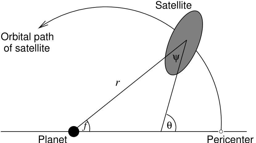
Figure 1: Geometry of a body in a spin-orbit resonance: $\theta$ is the angle between the ellipsoid’s longest axis and a reference line, chosen for the sake of simplicity to coincide with the semi-major axis of the satellite’s fixed orbit.

The spin-orbit problem is discussed in modern texts such as Murray & Dermott (1999) or Sussman & Wisdom (2001), so here we only cover the essentials briefly. In the planar problem, pictured in Fig. 1, the angle $f$ is the true anomaly while $\psi$ is the angle between the satellite-planet line and central axis of the satellite. It is clear that $\theta=f+\psi$. Neglecting tidal torques, the resulting equation of motion for $\theta$ is (Goldreich & Peale, 1966)

$$\ddot{\theta}=-{\frac{1}{2}}\,\alpha^{2}\,n^{2}\,{\frac{a}{r^{3}}}\,\sin{(2\,(\theta-f))}$$ (1)

where $a$ is the satellite’s semi-major axis, $r$ measures the satellite’s radial distance to the planet, and $n$ is the mean motion (i.e. angular orbital frequency). The asphericity parameter $\alpha$ is defined in terms of the moments of inertia $A\leq B\leq C$ by

$$\alpha=\sqrt{\frac{3\,(B-A)}{C}}.$$ (2)

The equation of motion Eq. (1) is explicitly integrable in two cases: (i) when the satellite is oblate i.e. $A=B$, there is zero torque indicating a freely rotating body, or (ii) when the orbit is circular, which corresponds to a pendulum equation.

It is easy to see that Eq. (1) is equivalent to the Hamiltonian

$$H(p,\,q,\,t)=\frac{p^{2}}{2}-\frac{\alpha^{2}}{4\,r^{3}}\,\cos{(2\,(q-f))}$$ (3)

where $f=f(t)$, $r=r(t)$, and $q\equiv\theta$. Units have been chosen such that $a=n=1$ and hence $2\,\pi$ corresponds to an orbital period. The Hamiltonian can be rendered autonomous by the standard device of extending the phase space. The equivalent autonomous Hamiltonian is

$$H(p_{1},\,p_{2};\,q_{1},\,q_{2})=\frac{p_{1}^{2}}{2}+p_{2}-\frac{\alpha^{2}}{4\,r^{3}}\,\cos{(2\,(q_{1}-f))}.$$ (4)

Here $q_{1}=\theta,p_{1}=\dot{\theta},q_{2}=t$ (and also equals the mean anomaly in celestial mechanics), while $p_{2}$ has a value such that $H(p_{1},\,p_{2};\,q_{1},\,q_{2})=0$.

The Hamiltonian (Eq. (4)) depends on $q_{2}$ through $r$ and $f$. For perturbation theory we wish to make the $q_{2}$-dependence explicit. There are classical techniques for doing so, but here we introduce a new way which is well-suited to computer algebra.

Consider the expansion

$$\frac{1}{r^{3}}\,\exp{(2\,f\,i)}=\sum_{k}\,H_{k}(e)\,\exp{(k\,{q_{2}}\,i)},$$ (5)

which is a Fourier series in $q_{2}$ with Fourier coefficients

$$H_{k}(e)=\frac{1}{2\,\pi}\,\int_{0}^{2\,\pi}{\frac{1}{r^{3}}\,\exp{((2\,f-k\,{q_{2}})\,i})}\,{d{q_{2}}}.$$ (6)

Let us recall the standard expressions for Keplerian motion in terms of the auxiliary variable $E$ (called the eccentric anomaly in celestial mechanics):

$$r = 1-e\,\cos{E},$$

$$q_{2} = E-e\,\sin{E},$$ (7)

$$\tan{\frac{f}{2}} = \sqrt{\frac{1+e}{1-e}}\,\tan{\frac{E}{2}}.$$

From Eq. (2.1) we have $d{q_{2}}=r\,dE$, which lets us rewrite Eq. (6) as

$$H_{k}(e)=\frac{1}{2\,\pi}\,\int_{0}^{2\,\pi}{\frac{1}{r^{2}}\,\exp{((2\,f-k\,{q_{2}})\,i})}\,{dE},$$ (8)

thus making the integrand an explicit function of the integration variable. The integral (Eq. (8)) may be solved as a power series in $e$ for any given $k$; the integration is somewhat tedious by hand, but trivial using computer algebra. The answer will always be real. Now, multiplying the complex conjugate of Eq. (5) by $\exp{(2\,{q_{1}}\,i)}$ and taking the real part gives

$$\frac{1}{r^{3}}\,\cos{(2\,(q_{1}-f))}=\sum_{k}\,H_{k}(e)\,\cos{(2\,{q_{1}}-k\,{q_{2}})}.$$ (9)

The potential part of the Hamiltonian (Eq. (4)) is now expressed as a Fourier series in $q_{1},q_{2}$ with coefficients $H_{k}(e)$ given by Eq. (8). The $H_{k}(e)$ themselves are power series in the eccentricity. They are credited in the literature to Cayley (1861) and we will refer to them as Cayley coefficients. They are tabulated in Table 1 of Goldreich & Peale (1966) and Table 2.1 of Celletti (1990a).

Thus the two degree of freedom autonomous Hamiltonian is

$$H(p_{1},\,p_{2};\,q_{1},\,q_{2})=\frac{{{p_{1}}}^{2}}{2}+{p_{2}}-\frac{\alpha^{2}}{4}\,\sum_{k=k_{\rm min}}^{{k_{\rm max}}}\,H_{k}(e)\,\cos{(2\,{q_{1}}-k\,{q_{2}})}.$$ (10)

Under this guise, the $1:1$ resonance with $k=2$ has the argument $\cos{(2\,{q_{1}}-2\,{q_{2}})}$; similarly, $k=3$ for the $3:2$ commensurability, and so the associated argument is $\cos{(2\,{q_{1}}-3\,{q_{2}})}$.

A body with low $e$ generally has as its final spin state the synchronous lock: this is dictated by the form of the Cayley coefficient $H_{2}(e)$, which in the limit as $e\rightarrow 0$, tends towards unity. Moreover the leading term in the $e-$series decays as ${\it O}(e^{|{k-2}|})$. So for small values of the eccentricity, it is reasonable to focus on the dominant resonances, namely the $1:1$ and the $3:2$, though several adjacent resonances must also be considered, not least to permit study of the effects caused by small divisors. For increasing eccentricity however, the presence of higher order $e$ terms in the expansion is crucial – these are now the prominent terms, substantially larger than their counterparts at lower order in $e$. Indeed, the higher the eccentricity, the longer it takes the series to converge.

To illustrate the preceding argument, in Table 1 we have tabulated the Cayley coefficients for selected solar system bodies. We also include an example of a highly eccentric object. While Mercury’s eccentricity is usually considered to be rather sizable, as far as this analysis is concerned, it falls into the low $e$ category. On the other hand, Nereid’s exceptionally high eccentricity of $e=0.75$ affords substantial significance to Cayley coefficients at growing distance from the traditionally strongest coupling; that is, the synchronous state.

2.2 Driven Pendulum

Our perturbative calculations with the Hamiltonian of Eq. (10) contain a minimum of four terms in the sum. At second order, the resulting expressions span several pages. Rather than mask the underlying simplicity of the perturbative scheme in such a mess, we choose instead a simple example to illustrate the mechanics of perturbation theory in the form of Lie transforms. The driven pendulum is a double pendulum – see Fig. 2 – with inner pendulum driven at unit angular frequency. Its Hamiltonian is

$$H(p_{1},\,p_{2};\,q_{1},\,q_{2})=\frac{p_{1}^{2}}{2}+p_{2}-{\alpha}\,\cos{q_{1}}-{\beta}\,\cos{(q_{1}-q_{2})}.$$ (11)

which is quite similar to the spin-orbit Hamiltonian, with the angles $q_{1}$ and $q_{2}$ being analogous to the orientation angle and orbital phase (mean anomaly) respectively. For a derivation of Eq. (11) see the Appendix. A different driven pendulum, having one more driving term, is considered in Sussman & Wisdom (2001).

3 Perturbation Theory

3.1 Resonant Integrals

An important property of Hamiltonian systems is the following: If $H$ depends on $q_{1}$ and $q_{2}$ only through the combination $l\,q_{1}-k\,q_{2}$, then ${k}\,{p_{1}}+{l}\,{p_{2}}$ will be a constant of the motion. Various forms of this statement appear in the literature – see for instance Theorem 2 of Gustavson (1966), but here we provide a simple proof.

Given any coprime integers $k,\,l$, we can always find integers $i,\,j$, such that the matrix

$$M=\begin{pmatrix}i&j\\ k&l\end{pmatrix}$$ (12)

has unit determinant. We can then define

$$\begin{pmatrix}P_{1}\\ P_{2}\end{pmatrix} = \begin{pmatrix}i&j\\ k&l\end{pmatrix}\begin{pmatrix}p_{1}\\ p_{2}\end{pmatrix}$$ (13)

$$\begin{pmatrix}Q_{1}\\ Q_{2}\end{pmatrix} = \begin{pmatrix}l&-k\\ -j&i\end{pmatrix}\begin{pmatrix}q_{1}\\ q_{2}\end{pmatrix}.$$ (14)

The integer matrix of Eq. (14) is the inverse transpose of that in Eq. (13). This transformation is canonical (see e.g. Sect. 3 of Binney & Spergel (1984)).

Now if $H$ depends on $Q_{1}={l}\,q_{1}-{k}\,q_{2}$ but is cyclic in $Q_{2}$, then $P_{2}={k}\,p_{1}+{l}\,p_{2}$ will be a constant of the motion, often called the fast action. $Q_{1}$ is the resonant (and hence slowly varying) angle and $Q_{2}$ is fast by comparison. As $(P_{1},\,P_{2})$ form the conjugate pair to $(Q_{1},\,Q_{2})$ they acquire the same nomenclature; thus $P_{1}$ is the slow or resonant action. Following averaging over $Q_{2}$, the fast action $P_{2}$ is constant.

Let us illustrate the conservation of $P_{2}$ by considering the Hamiltonian

$$H=\frac{1}{2}\,p_{1}^{2}+p_{2}+{\kappa}\,\cos{(n\,(l\,q_{1}-k\,q_{2}))}$$ (15)

with $H=0$. This gives us

$$p_{2}=-\frac{1}{2}\,p_{1}^{2}-{\kappa}\,\cos{(n\,(l\,q_{1}-k\,q_{2}))}.$$ (16)

Making use of this equation and our earlier result that ${k}\,p_{1}+{l}\,p_{2}={\rm constant}$ we have

$$\frac{1}{2}\,\left(p_{1}-\frac{k}{l}\right)^{2}+{\kappa}\,\cos{\left(n\,l\,\left(q_{1}-\frac{k}{l}\,q_{2}\right)\right)}={\rm constant}$$ (17)

which is a pendulum equation. If we now introduce a resonant angle $\gamma\equiv q_{1}-(k/l)\,q_{2}$, we will recover the pendulum equation in Eq. (5) of Goldreich & Peale (1966).

The well-known overlap criterion of Chirikov (1979) corresponds to the overlap of oscillations of pendulum equations resulting from two or more resonance terms. This is considered a diagnostic for the onset of large-scale chaos.

3.2 Lie Transforms

Hamiltonian perturbation theory is based on transforming a Hamiltonian $H(p,\,q)$ into a so-called Kamiltonian $K(p^{\prime},\,q^{\prime})$ which is easier to solve. Lie transforms are the standard technique for carrying out the desired transformation, and are described in several books, e.g. Sussman & Wisdom (2001). We summarize the Lie transform method here, following Cary (1981).

Let us consider a transformation $T$ whose effect is

$$T\,K(p,\,q)=K(p^{\prime},\,q^{\prime})$$ (18)

where $K$ represents an arbitrary functional form. In particular,

$$T\,{p}=p^{\prime},\quad T\,{q}=q^{\prime}.$$ (19)

Now, if we define

$$H(p,\,q)=K(p^{\prime},\,q^{\prime})$$ (20)

then $T\,K=H$ essentially changes the functional form of the new function $K$ to the functional form of the old function, $H$.

Thus far, $T$ could be any transformation. But for perturbation theory we are interested in a canonical transformation $T$ derived from a generating function $W$, depending on a perturbation parameter $\epsilon$ such that as $\epsilon\rightarrow 0$, $W\rightarrow 0$ and $T\rightarrow 1$. Accordingly, we now introduce the generating function

$$W=\epsilon\,W_{1}+{\epsilon^{2}}\,W_{2}$$ (21)

and define linear operators $L_{1}$ and $L_{2}$ such that

$$L_{1}\,F\equiv\sum_{i}^{n}\left(\frac{\partial F}{\partial q_{i}}\frac{\partial W_{1}}{\partial p_{i}}-\frac{\partial F}{\partial p_{i}}\frac{\partial W_{1}}{\partial q_{i}}\right)$$ (22)

and similarly for $L_{2}$. Here $n$ is the number of degrees of freedom. The transformation $T$ is now expressed as the operator

$$T=1+\epsilon\,L_{1}+{\epsilon^{2}}\,\left(\text@frac{1}{2}\,L_{1}^{2}+L_{2}\right)+\ldots.$$ (23)

To ${\it O}(\epsilon^{2})$, $K$ is related to $H$ as follows:

$$T\left(K_{0}+{\epsilon}\,K_{1}+{\epsilon^{2}}\,K_{2}\right) = H_{0}+{\epsilon}\,H_{1}+{\epsilon^{2}}\,H_{2},$$

$$\left(1+{\epsilon}\,L_{1}+{\epsilon^{2}}\,\left(\framebox{$\frac{1}{2}$}L_{1}^{2}+L_{2}\right)\right)\left(K_{0}+{\epsilon}\,K_{1}+{\epsilon^{2}}\,K_{2}\right) = H_{0}+{\epsilon}\,H_{1}+{\epsilon^{2}}\,H_{2}.$$ (24)

Equating powers of $\epsilon$ we obtain the series of equations

$$K_{0} = H_{0},$$ (25)

$$L_{1}K_{0} = H_{1}-K_{1},$$ (26)

$$L_{2}K_{0} = H_{2}-\framebox{$\frac{1}{2}$}L_{1}\left(H_{1}+K_{1}\right)-K_{2}.$$ (27)

In a first order perturbative calculation we choose $K_{1}$ so that it contains only secular and resonant terms (and hence has a constant of motion, which can be calculated) and construct a $W_{1}$ so as to solve Eq. (26). At second order, we choose $K_{2}$ so as to contain only secular and resonant terms, and construct a $W_{2}$ so as to solve Eq. (27). The appropriate choice of $K_{1}$ and $K_{2}$ avoids small denominators.

At this point it is worth clarifying our use of subscripts. For the most part, subscripts ${0,\,1,\,2}$ respectively indicate zeroth, first, and second order terms. On the other hand, the subscripts on the generalized coordinates $(p_{1},\,p_{2};\,q_{1},\,q_{2})$ are unrelated to order: rather they were introduced upon extension of the phase space.

3.3 Example: Driven Pendulum

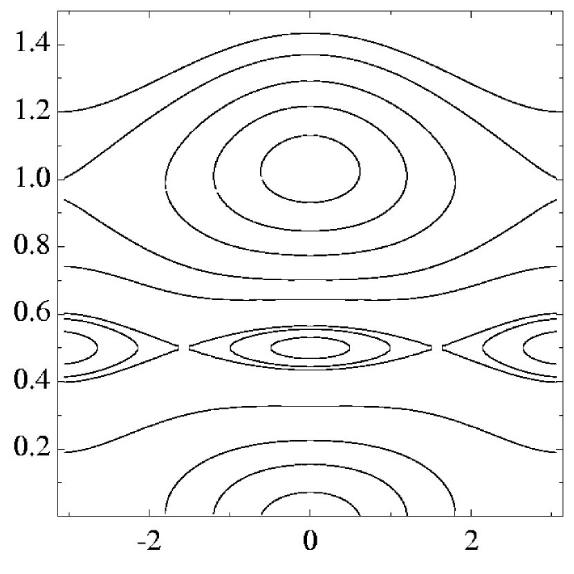
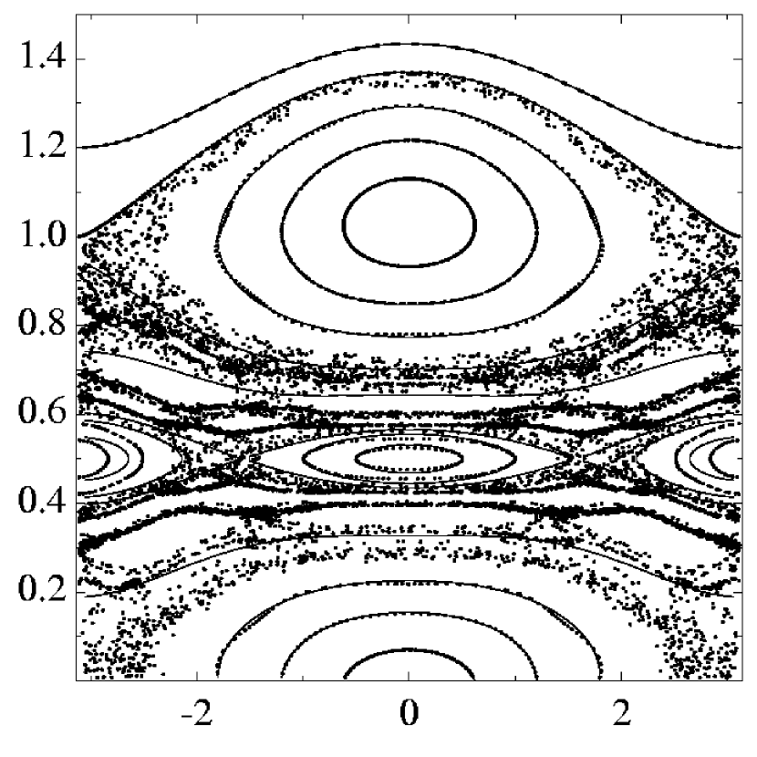
Figure 3: Upper panel: Contours of the fast action (slice chosen at $q_{2}=0$) for the driven pendulum with $\alpha=\beta=0.03$. Lower panel: Numerical surface of section for the driven pendulum for the same parameters. The second order $1:2$ resonance is clearly visible centered on $p_{1}=0.5$. Also evident are the first order $0:1$ and $1:1$ states. The horizontal axis measures $q_{1}$ while the vertical axis measures $p_{1}$.

We now work through an example to illustrate how to implement Lie transform perturbation theory, illustrating how a perturbative model of the driven pendulum fares in relation to numerical integration in Fig. 3. We find that the perturbative solution approximates well both the location and extent of the islands.

The Hamiltonian for the driven pendulum was defined in Eq. (11). For algebraic convenience we make the replacements $\alpha\rightarrow\epsilon\,\alpha,\beta\rightarrow\epsilon\,\beta$ (and set $\epsilon=1$ for numerical work), which lets us write

$$H_{0} = \frac{p_{1}^{2}}{2}+p_{2},$$

$$H_{1} = -{\alpha}\,\cos{q_{1}}-{\beta}\,\cos{(q_{1}-q_{2})},$$ (28)

$$H_{2} = 0.$$ (29)

3.3.1 Driven pendulum: $1:1$ resonance

Let us start by considering a first order resonance. $H_{0}$ by construction is integrable. From Eq. (25)

$$K_{0}=H_{0}=\frac{p_{1}^{2}}{2}+p_{2}.$$ (30)

Clearly $K_{0}$ is cyclic in $q_{1}$ and $q_{2}$. $K_{1}$ is chosen such that $H_{1}-K_{1}$ will have no resonant or secular terms. In other words, we take any terms in $H_{1}$ that are either independent of $q_{1},\,q_{2}$ or involve the resonant argument (in this case $q_{1}-q_{2}$) and copy them into $K_{1}$. Thus we choose

$$K_{1}(p_{1},\,p_{2};\,q_{1},\,q_{2})=-\beta\,\cos{({q_{1}}-{q_{2}})}.$$ (31)

With this choice Eq. (26) becomes

$${L_{1}}{K_{0}}=-{\alpha}\,\cos{q_{1}}.$$ (32)

To solve this equation for the first order generating function $W_{1}$, we first observe that if

$$W_{1}=-\frac{A\,\sin{(m\,q_{1}+n\,q_{2})}}{m\,p_{1}+n}$$ (33)

and $K_{0}$ is given by Eq. (30), then

$$L_{1}\,K_{0}=A\,\cos{(m\,q_{1}+n\,q_{2})}.$$ (34)

Comparing Eqs. (34) and (32), and then plugging into Eq. (33) gives

$$W_{1}(p_{1},\,p_{2};\,q_{1},\,q_{2})=\frac{\alpha\,\sin{({q_{1}})}}{{p_{1}}}.$$ (35)

Note that had we opted to assign $K_{1}=0$ rather than the value given in Eq. (31) then $W_{1}$ would have included another term (see Eq. (46)) with denominator $p_{1}-1$. Clearly this would introduce a singularity in the transformation at exact resonance, and a small denominator near resonance. This is of course the problem of small divisors which in this instance we have avoided.

Though the $1:1$ is a first order resonance, we develop the theory to second order. Following the above choices for $K_{1}$ and $W_{1}$ we have

$$H_{2}-\text@frac{1}{2}\,L_{1}(H_{1}+K_{1})=\frac{\alpha^{2}}{4\,{{p_{1}}}^{2}}-\frac{\alpha^{2}\,\cos{(2\,{q_{1}})}}{4\,{{p_{1}}}^{2}}-\frac{\alpha\,\beta\,\cos{(2\,{q_{1}}-{q_{2}})}}{2\,{{p_{1}}}^{2}}+\frac{\alpha\,\beta\,\cos{({q_{2}})}}{2\,{{p_{1}}}^{2}}.$$ (36)

We choose $K_{2}$ to consist of all secular and resonant terms in this expression, following the same principle as we did in choosing $K_{1}$. In fact, there is only one secular term involved here, giving us

$$K_{2}=\frac{\alpha^{2}}{4\,{{p_{1}}}^{2}}.$$ (37)

Having thus chosen $K_{2}$, the right-hand side of Eq. (27) will consist of the last three terms in Eq. (36). We now solve Eq. (27) term by term for $W_{2}$, just as we solved Eq. (26) for $W_{1}$. We get

$$W_{2}=\frac{\alpha^{2}\,\sin{(2\,q_{1})}}{8\,p_{1}^{3}}+\frac{\alpha\,\beta\,\sin{(2\,q_{1}-q_{2})}}{2\,p_{1}^{2}\,(2\,p_{1}-1)}-\frac{\alpha\,\beta\,\sin{(q_{2})}}{2\,p_{1}^{2}}$$ (38)

and rewriting quotients as partial fractions gives

$$W_{2} = \frac{\alpha^{2}\,\sin{(2\,{q_{1}})}}{8\,{{p_{1}}}^{3}}-\frac{\alpha\,\beta\,\sin{(2\,{q_{1}}-{q_{2}})}}{{p_{1}}}+$$ (39)

$$\frac{2\,\alpha\,\beta\,\sin{(2\,{q_{1}}-{q_{2}})}}{2\,{p_{1}}-1}-\frac{\alpha\,\beta\,\left(\sin{(2\,{q_{1}}-{q_{2}})}+\sin{({q_{2}})}\right)}{2\,{{p_{1}}}^{2}}.$$

Again, we see the presence of a small denominator in the third term in $W_{2}$. However, this particular factor is acceptable since it is associated with the $2:1$ resonance, and is thereby outside the domain of the $1:1$ resonance.

Thus far $H(p_{1},\,p_{2};\,q_{1},\,q_{2})$ has essentially undergone a canonical transformation to produce $K(p^{\prime}_{1},\,p^{\prime}_{2},\,q^{\prime}_{1}-q^{\prime}_{2})$. From Sect. 3.1 we know that for the $1:1$ resonance we are now considering, $p^{\prime}_{1}+p^{\prime}_{2}$ will be the constant fast action. Since $T\,p=p^{\prime}$ we may derive an expression for this fast action

$$C(p_{1},\,p_{2};\,q_{1},\,q_{2})\equiv T(p_{1}+p_{2})={\rm constant}.$$ (40)

The leading order fast action $C_{0}$ is simply $p_{1}+p_{2}$. Using the condition $H(p_{1},\,p_{2};\,q_{1},\,q_{2})=0$ to eliminate $p_{2}$ we have

$$C_{0}={p_{1}}-\frac{{{p_{1}}}^{2}}{2}+\alpha\,\cos{({q_{1}})}+\beta\,\cos{({q_{1}}-{q_{2}})}.$$ (41)

In averaging theory the $\alpha\,\cos{({q_{1}})}$ term would be jettisoned, since it is a non-resonant or fast term. The first order correction to the fast action is

$$C_{1}=-\frac{\alpha\,\cos{({q_{1}})}}{{p_{1}}}.$$ (42)

Similarly, $C_{2}$ is the second order contribution. Observe that the first order terms are proportional to $\alpha$ and $\beta$ whereas at second order cross-terms are introduced.

$$C_{2} = \frac{-\alpha^{2}\,\left(2+\cos{(2\,{q_{1}})}\right)}{4\,{{p_{1}}}^{3}}+\frac{\alpha\,\beta\,\cos(2\,{q_{1}}-{q_{2}})}{{p_{1}}}-\frac{2\,\alpha\,\beta\,\cos(2\,{q_{1}}-{q_{2}})}{2\,{p_{1}}-1}$$ (43)

$$+\frac{\alpha\,\beta\,\left(\cos(2\,{q_{1}}-{q_{2}})+\cos({q_{2}})\right)}{2\,{{p_{1}}}^{2}}.$$

Thus the complete expression for the fast action at second order is given by

$$C=C_{0}+C_{1}+C_{2}.$$ (44)

3.3.2 Driven pendulum: $2:1$ resonance

The $2:1$ resonance is second order, so called because the perturbation must be extended to second order in order to produce it. The resonant argument $2\,q_{1}-q_{2}$ is absent from $H_{1}$, hence we choose

$$K_{1}(p_{1},\,p_{2};\,q_{1},\,q_{2})=0$$ (45)

Now Eq. (26) becomes ${L_{1}}{K_{0}}=H_{1}-K_{1}=-{\alpha}\,\cos{q_{1}}-{\beta}\,\cos{(q_{1}-q_{2})}$. We solve this equation for $W_{1}$, taking our cue from Eqs. (33) and (34) as before, obtaining

$$W_{1}(p_{1},\,p_{2};\,q_{1},\,q_{2})=\frac{\alpha\,\sin{({q_{1}})}}{{p_{1}}}+\frac{\beta\,\sin{({q_{1}}-{q_{2}})}}{{p_{1}}-1}.$$ (46)

$K_{2}$ is composed of the appropriate secular and resonant terms again:

$$K_{2}=\frac{-\beta\,\left(-\beta+\alpha\,\cos{(2\,{q_{1}}-{q_{2}})}\right)}{4\,{\left({p_{1}}-1\right)}^{2}}+\frac{\alpha\,\left(\alpha-\beta\,\cos{(2\,{q_{1}}-{q_{2}})}\right)}{4\,{{p_{1}}}^{2}}.$$ (47)

Solving Eq. (27) for this case gives

$$W_{2}=\frac{\alpha^{2}\,\sin{(2\,{q_{1}})}}{8\,{{p_{1}}}^{3}}+\frac{\beta^{2}\,\sin{(2\,{q_{1}}-2\,{q_{2}})}}{8\,{\left({p_{1}}-1\right)}^{3}}-\frac{\alpha\,\beta\,\sin{({q_{2}})}}{4\,{\left({p_{1}}-1\right)}^{2}}-\frac{\alpha\,\beta\,\sin{({q_{2}})}}{4\,{{p_{1}}}^{2}}.$$ (48)

The $2:1$ resonant variables are obtained in the same manner as for $1:1$. In this instance, the leading order fast action has the form

$$C_{0}=p_{1}-{p_{1}^{2}}+2\,\alpha\,\cos{(q_{1})}+2\,\beta\,\cos{(q_{1}-q_{2})}.$$ (49)

The first order correction is

$$C_{1}=-{\frac{\alpha\,\cos{\left({q_{1}}\right)}}{{p_{1}}}}+{\frac{\beta\,\cos{\left({q_{1}-q_{2}}\right)}}{{p_{1}}-1}}.$$ (50)

As before, $C_{2}$ is the second order contribution,

$$C_{2} = \frac{-\left(\alpha^{2}\,\left(2+\cos(2\,{q_{1}})\right)\right)}{4\,{{p_{1}}}^{3}}+\frac{\beta^{2}\,\left(2+\cos{(2\,{q_{1}}-2\,{q_{2}})}\right)}{4\,{\left({p_{1}}-1\right)}^{3}}-\frac{\alpha\,\beta\,\cos{(2\,{q_{1}}-{q_{2}})}}{{p_{1}}-1}+$$ (51)

$$\frac{\alpha\,\beta\,\cos{(2\,{q_{1}}-{q_{2}})}}{{p_{1}}}+\frac{\alpha\,\beta\,\left(\cos{(2\,{q_{1}}-{q_{2}})}+\cos{({q_{2}})}\right)}{2\,{\left({p_{1}}-1\right)}^{2}}+$$

$$\frac{\alpha\,\beta\,\left(\cos{(2\,{q_{1}}-{q_{2}})}+\cos{({q_{2}})}\right)}{2\,{{p_{1}}}^{2}}.$$

3.3.3 Driven pendulum: Surface of section

In Fig. 3 we show a comparison between second order perturbation theory and a numerical integration of the Hamiltonian Eq. (11).

The curves in the upper panel are curves of the second order fast action $C_{0}+C_{1}+C_{2}$ at $q_{2}$. In the upper part of the plot – the vicinity of the $1:1$ resonance – the individual terms come from Eqs. (41) to (43). In the middle part of the plot – the neighborhood of the $1:2$ resonance – the individual terms come from Eqs. (49) to (51). The lower part of the plot is the $0:1$ ‘resonance’ region; here the terms in $C_{0},\,C_{1},\,C_{2}$ are calculated in the same way, but we omit the details for brevity.

To produce the lower panel we started a numerical integration from a random point on each of the perturbative curves and then followed an orbit for several crossings of the plane $q_{2}=0$, plotting the value of $(p_{1},\,q_{1})$ at each crossing.

The analogous figure for first order perturbation theory would contain the contours of $C_{0}+C_{1}$ at $q_{2}=0$. Finally, the analogous figure for averaging theory would have contours of $C_{0}$ with any non-resonant periodic terms discarded, also at $q_{2}=0$.

4 Results

We now proceed to the spin-orbit Hamiltonian (Eq. (10)), defining the perturbation parameter as $\epsilon={\alpha^{2}}/4$. We set $k_{\rm min}=1$ and $k_{\rm max}=4$, except for one case (Hyperion) when we increase $k_{\rm max}$ to 6.

In Table 2 we list the spin-orbit parameters for selected objects. In fact $\alpha$ exceeds unity for a significant fraction of solar system bodies, including many asteroids; for instance, 4179 Toutatis has $\alpha\approx 1.35$ and 243 Ida has $\alpha\approx 1.44$. Bearing in mind that perturbation theory is only valid for small $\epsilon$, it is important to find what regimes of $\alpha,e$ our perturbative model is useful for.

4.1 The useful regime for perturbation theory

Fig. 4 is a sketch of the different regimes of $\alpha,\,e$. (The curves in this figure are not precise boundaries; they are approximate indications based on examining the results of perturbation theory and numerical integration for many different parameter values.) The labeled regions are as follows.

A:

For $\alpha\lesssim 0.05$ or $e\lesssim 0.1$ phase space consists of non-resonant spins and first order resonant islands, with no significant second order resonances or chaos. Averaging gets the structure qualitatively right, while first and second order perturbation theory make some quantitative improvement.

B:

For $0.05\lesssim\alpha\lesssim 0.2$ and $e\gtrsim 0.1$ there are both first and second order islands. Second order perturbation theory successfully recovers the second order islands, whereas averaging and first order perturbation theory are limited to the first order islands.

C:

For $0.2\lesssim\alpha\lesssim 0.3$ and $e\gtrsim 0.1$ there are significant chaotic regions along with first and second order islands.

D:

For $0.3\lesssim\alpha\lesssim 0.5$ or $0.1\lesssim e\lesssim 0.2$ chaos wipes out the second order islands. First order islands persist, but gradually diminish in size. Averaging and first order perturbation theory are still useful outside the chaotic regions.

E:

For $\alpha\gtrsim 0.5$ and $e\gtrsim 0.2$ phase space is mostly chaotic, except for very small resonant islands.

Second order perturbation theory is important in regions B and C, where $0.05\lesssim\alpha\lesssim 0.3$ and $e\gtrsim 0.1$. We are not aware of any objects whose parameters are known that fall in regions B and C, but it is possible that as more $\alpha$ values are ascertained such objects will be identified. It seems likely that bodies inhabiting a second order spin-orbit resonance do exist.

To illustrate the results of our perturbative calculations, let us first consider a hypothetical body roughly at the boundary of regions B and C; we choose $\alpha=e=0.2$ and consider its surface of section in detail in Fig. 5.

Fig. 5a shows the second order perturbative model (that is, contours of the second order fast action) covering first and second order primary resonances from $1:2$ through $2:1$. First order islands will have stable equilibria at $\theta=0,\pm{\pi}$ if $H_{k}(e)>0$, and at $\pm{\pi}/{2}$ for $H_{k}(e)<0$. Here the $1:2$ resonance is of the latter type because $H_{1}(e)<0$, whereas the $1:1$, $3:2$, and $2:1$ resonances are of the former type. For second order resonances, which here are $3:4$, $5:4$, and $7:4$, the situation is more complicated, but the same principle holds.

Comparison of Fig. 5a with 5b shows excellent agreement between second order perturbation theory model and numerical integrations through most of phase space. But perturbation theory naturally fails in the chaotic regions. Our perturbative model also fails to reproduce the chain of secondary islands surrounding the synchronous island in Fig. 5b; our model traces contours through the whole chain. We will discuss this issue in more detail below.

In Figs. 5c & 5d we show respectively the curves generated by the first order theory and by averaging. The averaging technique reasonably approximates the $1:1$ and $3:2$ zones at these parameters. First order perturbation theory improves on averaging in that asymmetries in the islands, unaccounted for by the averaging, now become apparent. But second order resonances are not reproduced.

We now consider another hypothetical body, this time in region E. We choose $\alpha=e=0.65$ and show results for it in Fig. 6. The averaging contours in Fig. 6a show resonance overlap, and large-scale chaos is expected. However, as Fig. 6b shows, chaos does not completely pervade phase space and many small resonant islands survive. Fig. 6c shows that second order perturbation theory can partially recover the $1:2$ islands even deep inside region E.

4.2 Particular objects

4.2.1 The Moon

As our closest neighbor in space, the Moon has been a natural stimulus and indeed testing ground for many theories of celestial mechanics. Its occupation of the synchronous $1:1$ state has allowed analysis of such tidal locking to be well studied for the many years prior to the confirmation that the same resonance (with respect to the corresponding parent planet) was shared by most other satellites in the solar system.

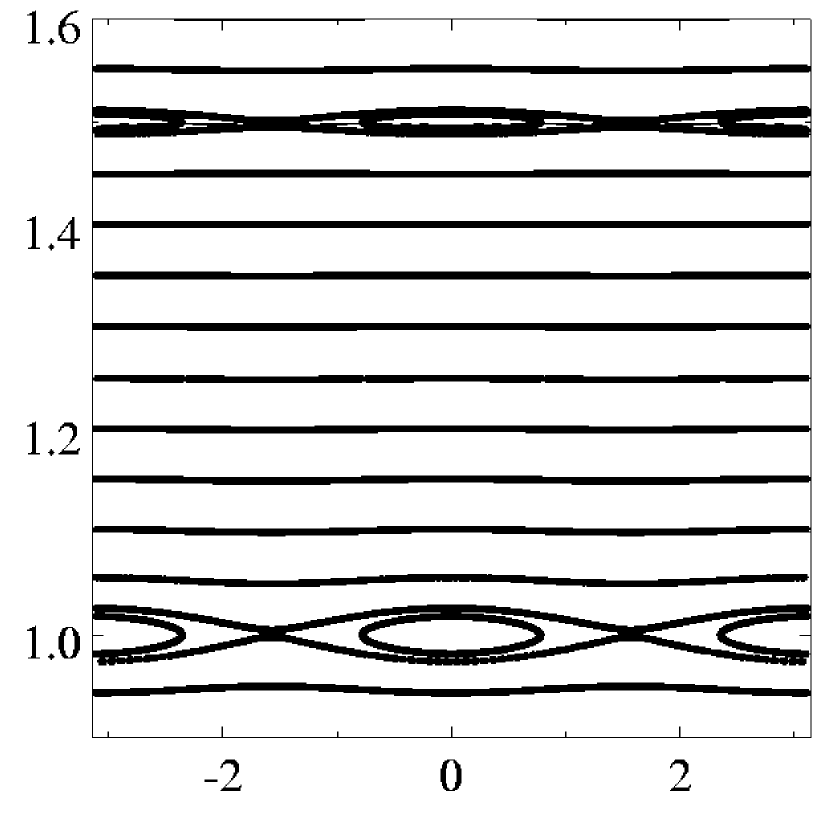
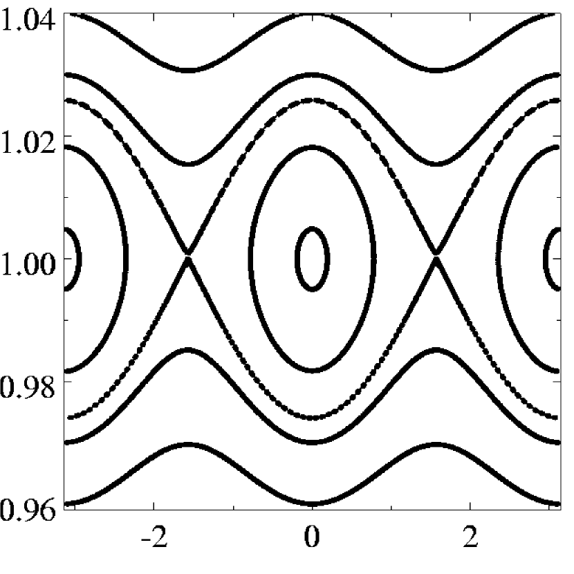
Figure 7: (a) Upper panel: Numerical surface of section (thick curves) for the Moon superimposed on second-order perturbative contours. The parameters are $\alpha=0.026;\,e=0.0549$. (b) Lower panel: Zoom of the synchronous zone. The horizontal axes measure $q_{1}=\theta$ and the vertical axes measure $p_{1}=\dot{\theta}/n$.

Since the Moon has a relatively low $e$ and $\alpha$, putting it in region A, we anticipate that even first order perturbation theory should provide a good match to the real system. Indeed, in Fig. 7 the second order perturbative and numerical surfaces of section are indistinguishable. The synchronous island and the $3:2$ islands are the only commensurabilities evident in the range plotted. We observe that in this instance there is scarcely any chaos bordering the separatrix.

4.2.2 Mercury

Let us investigate whether the agreement is comparable in the case of Mercury which has a more elongated orbit than that of the Moon, and is trapped in the $3:2$ resonance. It remains the only known example of a non-synchronous primary resonance in our solar system. Mercury spins on its axis once every $59.65$ days while taking roughly $1.5$ times as long to complete a single orbit in $87.97$ days. The current eccentricity is $e=0.206$, but Correia & Laskar (2004) show that chaotic evolution of Mercury’s orbit is capable of driving $e$ to $\simeq 0.45$. The asphericity is $\alpha=0.0187$ putting Mercury in region A.

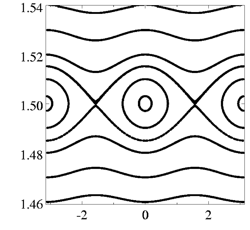
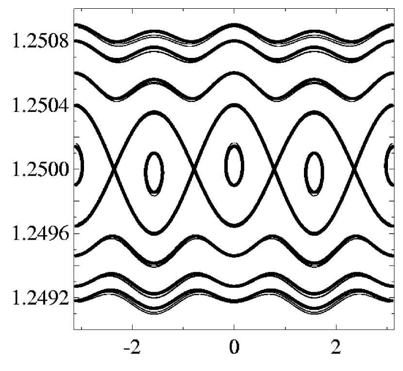
Figure 8: (a) Upper panel: Numerical surface of section for Mercury (thick curves) superimposed on the second-order perturbative contours. Only the region around the $3:2$ state is plotted. (b) Lower panel: Similar, but near the second-order $5:4$ resonance. Note the change in scale from Fig. 8a. The parameters are $\alpha=0.0187;\,e=0.206$. The horizontal axes measure $q_{1}=\theta$ and the vertical axes measure $p_{1}=\dot{\theta}/n$.

In Fig. 8 we illustrate the dynamics in the neighborhood of $3:2$ and $5:4$ resonances. The second order perturbative and numerical surfaces of section are almost indistinguishable. The second order $5:4$ resonance – though it exists – is tiny compared to the first order $3:2$ resonance, and this is typical of region A. We found that for Mercury’s low asphericity, the width of the $3:2$ resonance is remarkably insensitive to $e$. Also, the $5:4$ islands remain tiny even at $e\simeq 0.5$. Thus it is very improbable that Mercury would ever have been trapped in the $5:4$ or other second order resonance. The aforementioned proximity of Mercury’s rotation rate to the nominal location of the $5:4$ resonance seems to be a coincidence.

4.2.3 Hyperion

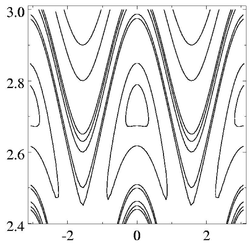
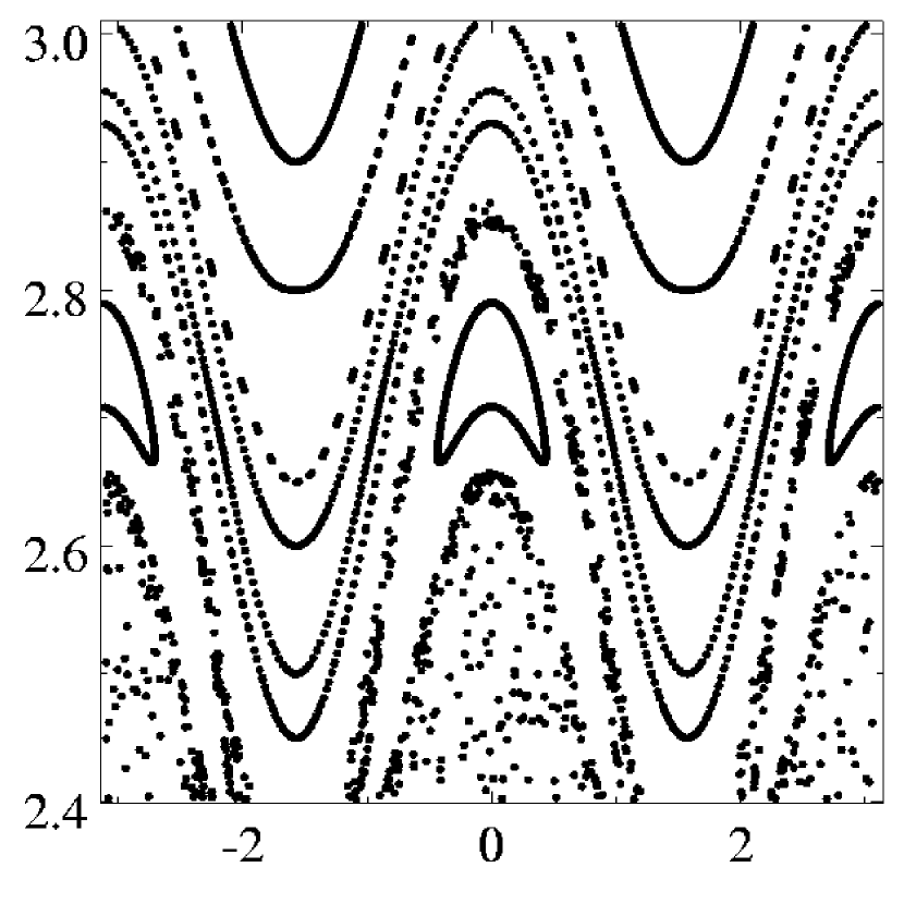
Figure 9: The $5:2$ islands for Hyperion. The upper panel shows the second-order perturbative result, while the lower panel is a numerical surface of section. The parameters are $\alpha=0.89;\,e=0.1236$. The horizontal axes measure $q_{1}=\theta$ and the vertical axes measure $p_{1}=\dot{\theta}/n$.

The chaotic nature of Hyperion’s rotation has already been mentioned in Sect. 1. Its large asphericity $\alpha\simeq 0.89$ together with eccentricity $e=0.1236$ puts Hyperion off the scale of Fig. 4 but at a location that would correspond to a position deep in region E. As evident from e.g. Fig. 1 of Black et al. (1995), the phase space is largely chaotic but has some small resonant islands. Our second order perturbative model recovers the $5:2$ resonant islands, as shown in Fig. 9 but does not succeed for islands below $\dot{\theta}/n\approx 2.5$. (In this example, we increased $k_{\rm max}$ in Eq. (10) from 4 to 6, because of the comparatively large perturbation.)

4.2.4 Enceladus

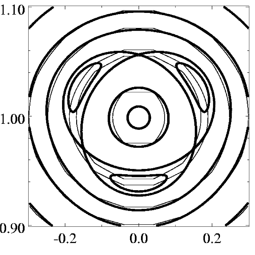
Figure 10: Numerical surface of section (thick curves) for Enceladus superimposed on the second-order perturbative contours. The parameters are $\alpha=0.336;\,e=0.0045$. The horizontal axis measures $q_{1}=\theta$ and the vertical axis measures $p_{1}=\dot{\theta}/n$. The $3:1$ secondary islands encircling the synchronous libration island is not reproduced by our theory: in their place exist concentric circles. This figure is analogous to Fig. 2 from Wisdom (2004).

The saturnian satellite Enceladus has a moderately high asphericity $\alpha=0.336$ but very low eccentricity $e=0.0045$, thus putting it in region A. It exhibits a secondary resonance, a phenomenon not allowed for in our perturbative model. Fig. 10 shows our results for the $1:1$ resonance in Enceladus. With relation to the secondary islands and their separatrix, we find that our perturbative model fails to resemble these lobes; instead concentric rings intersect these areas. On the other hand, Wisdom (2004) shows that the secondary resonances can be reproduced by an averaging model specifically designed for secondary resonances. To facilitate comparison, Fig. 10 has been chosen to have the same scales as Wisdom’s Fig. 2a.

We will now digress briefly to explain the difference between Wisdom’s approach and ours.

4.3 Secondary Resonance Dynamics

Let us return for a moment to the main Hamiltonian Eq. (10). Considering only the synchronous resonance, the Hamiltonian becomes

$$H(p_{1},\,p_{2};\,q_{1},\,q_{2})=\frac{{{p_{1}}}^{2}}{2}+{p_{2}}-\frac{\alpha^{2}}{4}\,\left(1-\frac{5\,e^{2}}{2}+\cdots\right)\,\cos{(2\,{q_{1}}-2\,{q_{2}})}.$$ (52)

Recall that we have taken

$$H_{0}(p_{1},\,p_{2};\,q_{1},\,q_{2})=\frac{{{p_{1}}}^{2}}{2}+{p_{2}},$$ (53)

as the unperturbed Hamiltonian and $\alpha^{2}/4$ as the perturbing parameter. The action-angle variables of $H_{0}$ are simply are $p_{1},\,p_{2},\,q_{1},\,q_{2}$. On the other hand Wisdom adopts

$$H_{0}^{W}(p_{1},\,p_{2};\,q_{1},\,q_{2})=\frac{{{p_{1}}}^{2}}{2}+{p_{2}}-\frac{\alpha^{2}}{4}\,\cos{(2\,{q_{1}}-2\,{q_{2}})}.$$ (54)

as the unperturbed Hamiltonian and $e$ as the perturbation. If this is done, the synchronous resonance appears already in the unperturbed dynamics, and then through perturbation theory the secondary resonances can be recovered. The complication is that the action-angle variables of $H_{0}^{W}$ are no longer $p_{1},\,p_{2},\,q_{1},\,q_{2}$ but non-elementary functions of them; moreover the perturbation must be expressed in terms of these new action-angles. Fortunately in the case of Enceladus, because of the small eccentricity, averaging is adequate and for averaging it is only necessary to extract one key term in the perturbation.

Developing first or second order Lie transform perturbation theory for secondary resonances is in principle possible but is a much more difficult task because of the complicated nature of the action-angle variables required.

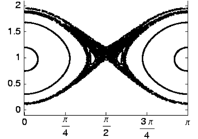
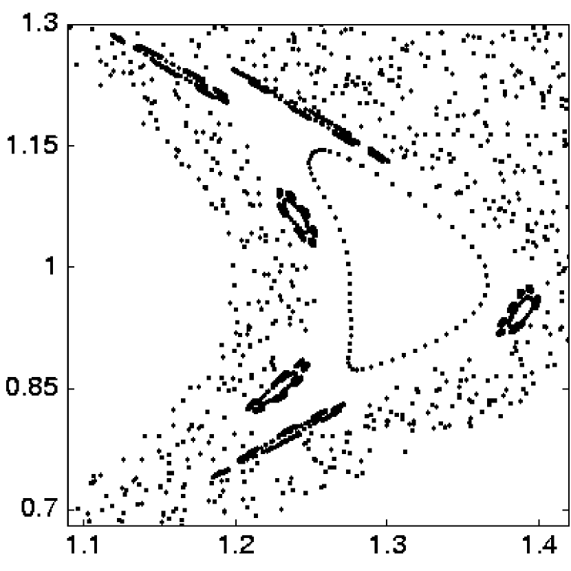
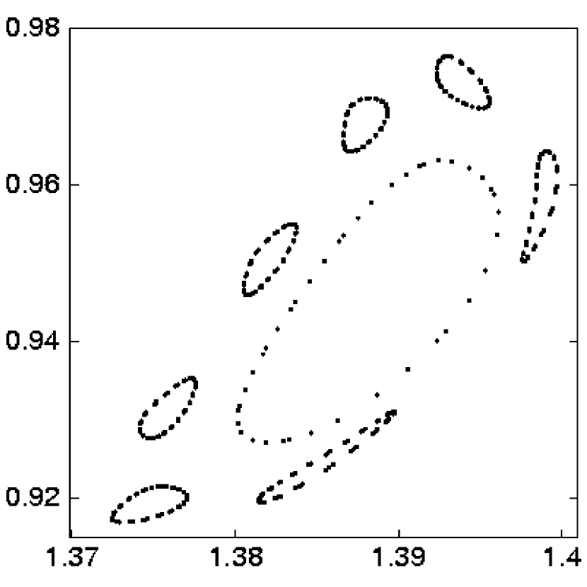
Figure 11: Upper panel: Numerical surface of section for Pandora. The parameters are $\alpha=0.89;\,e=0.0004$. Middle panel: Zooming in on the secondary island and its environs. Lower panel: Zooming in further in on a tertiary isle, itself encircled by seven quaternary islets. The horizontal axes measure $q_{1}=\theta$ and the vertical axes measure $p_{1}=\dot{\theta}/n$.

Secondary resonances are themselves part of a hierarchy which may extend down to smaller and smaller scales. As an illustration, we show a numerical surface of section for the saturnian satellite Pandora in Fig. 11. Zooming in successively, we see primary, secondary, tertiary, and quaternary resonant islands.

5 Conclusions

We have applied the technique of Lie transform perturbation theory to the planar spin-orbit problem, to second order. The full perturbative expressions are too long to include in the paper, but fortunately the main features of spin-orbit dynamics have analogs in the simpler problem of a driven double pendulum, which allows us to explain our perturbative method without excessive algebra.

We have compared our perturbative model to numerical integrations for various values of the asphericity parameter $\alpha$ and the orbital eccentricity $e$. If at least one of these is small ($\alpha\lesssim 0.05$ or $e\lesssim 0.1$) then only first order resonances are important and first order perturbation theory is adequate; Mercury and the Moon lie in this regime. If the tidal perturbations become too large ($\alpha\gtrsim 0.5$ and $e\gtrsim 0.2$) then the spin becomes chaotic and perturbation theory fails altogether; Hyperion is the best-known example. However, for intermediate perturbations ($0.05\leq\alpha\leq 0.3$ and $e>0.1$) second order resonances are possible and second order perturbation theory can reproduce them.

Our perturbative model is limited to primary resonances. In particular, Enceladus is thought to be in a secondary $3:1$ resonance around the primary synchronous resonance. Our model smooths over secondary resonances, putting Enceladus in an ordinary primary resonance. However, Wisdom (2004) has shown how to recast the problem so that the secondary resonance can be correctly reproduced in perturbation theory. Extending Wisdom’s model to second order is possible in principle, but very complicated.

So far, none of the objects whose asphericities may be found in the literature fall in the region of $\alpha,\,e$ where second order perturbation theory is particularly interesting, that is, regions B and C of Fig. 4. But there is no doubt that objects in the interesting parameter range do exist, and the possibility of objects being locked in second order resonances remains open.

Appendix A The driven pendulum

The Hamiltonian

$$H(p,\,q,\,t)=\frac{p^{2}}{2}-\alpha\,\cos{q}-\beta\,\cos{(q-t)}$$ (A1)

has been widely studied in the literature on the transition to chaos, e.g. Escande (1982). Several possible physical realizations of this Hamiltonian are known, typically involving electric or magnetic fields. Here we present another physical interpretation, which is very simple to visualize and is intuitively analogous to the the spin-orbit problem.

Our physical system is illustrated in Fig. 2. It is a double pendulum with two light rods and hinges and a single bob at the end. The inner pendulum (having length $b$, say) is made to circulate by an external motor at unit angular frequency. The outer pendulum (having length $l$, say) is free to librate or circulate. We can write the coordinates of the bob as

$$x = l\,\sin{q}+b\,\sin{t}$$ (A2)

$$y = -l\,\cos{q}-b\,\cos{t}.$$ (A3)

The Lagrangian for the bob can be written as

$$L(q,\,\dot{q},\,t)=\frac{b^{2}}{2}+\frac{l^{2}\,\dot{q}^{2}}{2}+g\,l\,\cos{q}+l\,b\,\dot{q}\,\cos{(q-t)}+g\,b\,\cos{t}.$$ (A4)

We now discard the first and last term. (The last term depends on neither of $q,\,\dot{q}$ and hence will not contribute to the equations of motion.) For algebraic convenience we also divide the Lagrangian by $l^{2}$ and introduce the parameters $\alpha=g/l,\,\beta=b/l$. As a result of all these changes Eq. (A4) can be replaced by

$$L(q,\,\dot{q},\,t)=\frac{\dot{q}^{2}}{2}+\alpha\,\cos{q}+\beta\,\dot{q}\,\cos{(q-t)}$$ (A5)

The interpretation of $\alpha,\,\beta$ is as follows: $\sqrt{\alpha}$ is the natural frequency of the outer pendulum relative to the driving frequency; $\sqrt{\beta}$ is the natural frequency of the outer pendulum relative to the inner. Hence $\alpha=\beta$ corresponds to the inner pendulum being driven at its natural frequency.

The Hamiltonian corresponding to $L$ in Eq. (A5) is

$$H(p,\,q,\,t)=\frac{\left(p-\beta\,\cos{(q-t)}\right)^{2}}{2}-\alpha\,\cos{q}.$$ (A6)

We can simplify (A6) using a canonical transformation. Inserting the generating function

$$S(p,\,Q)=p\,Q-\beta\,\sin{(Q-t)}$$ (A7)

in

$$p\,dq-H\,dt=P\,dQ-K\,dt+d(p\,q)-dS$$ (A8)

and comparing coefficients of the differentials, we obtain

$$K(P,\,Q,\,t)=\frac{P^{2}}{2}-\alpha\,\cos{Q}-\beta\,\cos{(Q-t)}.$$ (A9)

Using the standard trick of adding a dimension to remove the explicit time dependence, and changing notation as

$$P\rightarrow p_{1},\quad Q\rightarrow q_{1},\quad K\rightarrow-p_{2},\quad t\rightarrow q_{2}$$

gives us the Hamiltonian Eq. (11).

This system is roughly analogous to the spin-orbit problem if we take the inner pendulum as corresponding to the orbit and the outer pendulum to the spin.

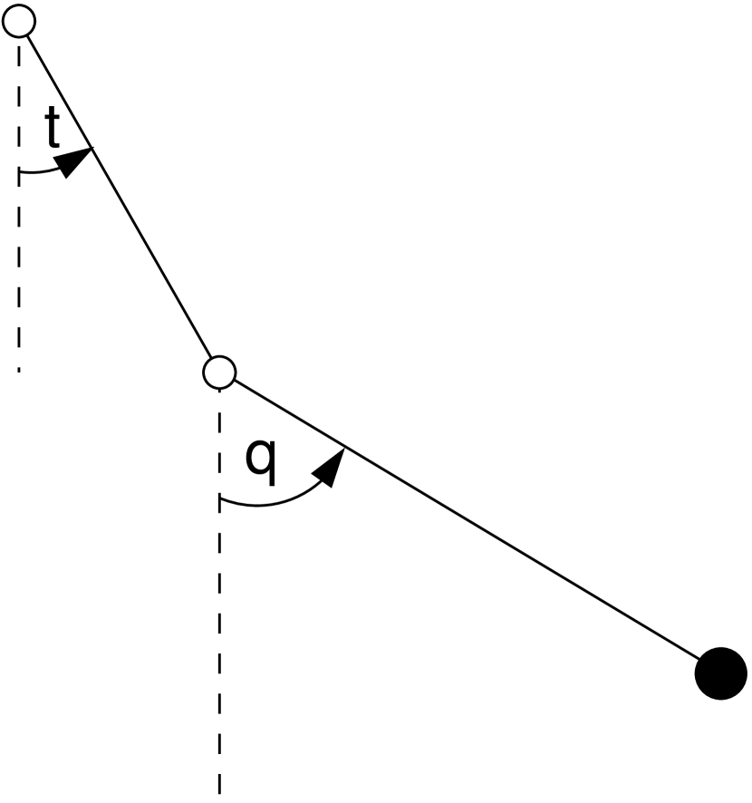
Figure 2: Mechanics of the driven double pendulum. The open circles correspond to weightless hinges while the filled circle indicates the mass.

Figure 4: Parameter regimes of the spin-orbit problem. A: non-resonant spins and first order resonant islands. B: similar to A, but with second order islands also present. C: like B but with significant chaos. D: second order islands overrun by chaos, first order islands remain. E: large-scale chaos with tiny or no resonant islands.

Figure 5: (a) Upper left panel: Surface of section, analogous to Fig. 3 but for the spin-orbit problem, illustrating the second order perturbation theory for the $1:2,\,3:4,\,1:1,\,5:4,\,3:2,\,7:4$ and $2:1$ resonances for $\alpha=0.2;\,e=0.2$. (b) Upper right panel: A numerical surface of section for the same parameters. (c) Lower left panel: First order result. (d) Lower right panel: Averaging result. In all our surfaces of section the horizontal axis measures $q_{1}=\theta$ and the vertical axis measures $p_{1}=\dot{\theta}/n$.

Figure 6: Surfaces of section for $\alpha=e=0.65$. (a) Upper panel: Contours from averaging, illustrating overlap between the $1:2$ and $1:1$ resonances. (b) Middle panel: Numerical surface of section showing large-scale chaos, but with numerous resonant islands. (c) Lower panel: Second order perturbative result partially recovering the $1:2$ islands. Note the change in scale from (a) and (b). The horizontal axes measure $q_{1}=\theta$ and the vertical axes measure $p_{1}=\dot{\theta}/n$.

Table 1: $H_{k}(e)$ to ${\it O}({e}^{4})$ for selected solar system bodies. Note that $H_{2}(e)\rightarrow 1$ as $e\rightarrow 0$.

$k$	Resonance	The Moon	Mercury	Hyperion	Enceladus	Nereid
-2	$-1:1$	$3.79\times{10}^{-7}$	$7.73\times{10}^{-5}$	$9.83\times{10}^{-6}$	$1.71\times{10}^{-11}$	$1.84\times{10}^{-2}$
-1	$-1:2$	$3.45\times{10}^{-6}$	$1.87\times{10}^{-4}$	$3.98\times{10}^{-5}$	$1.90\times{10}^{-9}$	$1.22\times{10}^{-2}$
1	$1:2$	$-2.74\times{10}^{-2}$	$-1.02\times{10}^{-1}$	$-6.17\times{10}^{-2}$	$-2.25\times{10}^{-3}$	$-3.52\times{10}^{-1}$
2	$1:1$	$0.992$	$0.895$	$0.962$	$1.000$	$-0.149$
3	$3:2$	$1.91\times{10}^{-1}$	$6.54\times{10}^{-1}$	$4.18\times{10}^{-1}$	$1.57\times{10}^{-2}$	$-6.18\times{10}^{-1}$
4	$2:1$	$2.54\times{10}^{-2}$	$3.26\times{10}^{-1}$	$1.25\times{10}^{-1}$	$1.72\times{10}^{-4}$	$-1.28$
5	$5:2$	$2.89\times{10}^{-3}$	$1.39\times{10}^{-1}$	$3.20\times{10}^{-2}$	$1.60\times{10}^{-6}$	1.90
6	$3:1$	$3.00\times{10}^{-4}$	$5.36\times{10}^{-2}$	$7.47\times{10}^{-3}$	$1.37\times{10}^{-8}$	3.27

Table 2: Physical parameters for selected solar system bodies.

Parameter	The Moon	Mercury	Hyperion	Enceladus	Pandora
$e$	0.0549	0.206	0.1236	0.0045	0.004
$\alpha$	0.026	0.0187	0.89	0.336	0.89

Note. — The parameter values are taken from the following sources: The Moon – Yoder (1995); Mercury – Rambaux & Bois (2004); Hyperion – Black et al. (1995); Enceladus – Wisdom (2004); Pandora – Wisdom (1987).

References

- Binney & Spergel (1984) Binney, J. & Spergel, D. 1984, MNRAS, 206, 159
- Black et al. (1995) Black, G. J., Nicholson, P. D., & Thomas, P. C. 1995, Icarus, 117, 149
- Blitzer (1979) Blitzer, L. 1979. Dynamics of Orbit-Orbit and Spin-Orbit Resonances: Similarities and Differences, in Natural and Artificial Satellite Motion, Proceedings of the International Symposium held at University of Texas at Austin, 1977, ed. Paul E. Nacozy and Sylvio Ferraz-Mello. (Austin: University of Texas Press)
- Cary (1981) Cary, J. R. 1981, Phys. Rep., 79, 129
- Cayley (1861) Cayley, A. 1861, MmRAS, 29, 191
- Celletti (1990a) Celletti, A. 1990a, J. of Appl. Math. and Phys. (ZAMP), 41, 174
- Celletti (1990b) Celletti, A. 1990b, J. of Appl. Math. and Phys. (ZAMP), 41, 453
- Celletti et al. (1998) Celletti, A., Della Penna, G. & Froeschlé, C. 1998, International Journal of Bifurcation and Chaos, 8, 2471
- Chauvineau & Métris (1994) Chauvineau, B. & Métris, G. 1994, Icarus, 109, 191
- Chirikov (1979) Chirikov, B. V. 1979, Phys. Rep., 52, 263
- Colombo (1965) Colombo, G. 1965, Nature, 208, 575
- Correia & Laskar (2004) Correia, A. C. M. & Laskar, J. 2004, Nature, 429, 848
- Escande (1982) Escande, D. F. 1982, Phys. Scr, T2, 126
- Goldreich & Peale (1966) Goldreich, P. & Peale, S. J. 1966, AJ, 71, 425
- Goldreich & Peale (1968) Goldreich, P. & Peale, S. J. 1968, ARA&A, 6, 287
- Goldstein (1980) Goldstein, H. 1980. Classical Mechanics, 2nd Edition. Addison-Wesley Pub. Co., Reading, Mass.
- Gustavson (1966) Gustavson, F. G. 1966, AJ, 71, 670
- Klavetter (1989) Klavetter, J. J. 1989, AJ, 97, 570
- Murray & Dermott (1999) Murray, C. D. & Dermott, S. F. 1999, Solar System Dynamics, Cambridge University Press, Cambridge
- Pettengill & Dyce (1965) Pettengill, G. H. & Dyce, R. B. 1965, Nature, 206, 1240
- Rambaux & Bois (2004) Rambaux, N. & Bois, E. 2004, A&A, 413, 381
- Sussman & Wisdom (2001) Sussman, G. J. & Wisdom, J. 2001, Structure and Interpretation of Classical Mechanics, MIT Press, Cambridge, Massachusetts
- Wisdom et al. (1984) Wisdom, J., Peale, S. J. & Mignard, F. 1984, Icarus, 58, 137
- Wisdom (1987) Wisdom, J. 1987, AJ, 94, 1350
- Wisdom (2004) Wisdom, J. 2004, AJ, 128, 484
- Yoder (1995) Yoder, C. F. 1995, Astrometric and Geodetic Properties of Earth and the Solar System, in Global Earth Physics. A Handbook of Physical Constants, ed. T. Ahrens (American Geophysical Union, Washington)