STATISTICAL MECHANICS OF THE SELF-GRAVITATING GAS: THERMODYNAMIC LIMIT, PHASE DIAGRAMS AND FRACTAL STRUCTURES

Abstract

We provide a complete picture of the non-relativistic self-gravitating gas at thermal equilibrium using Monte Carlo simulations, analytic mean field methods (MF) and low density expansions. The system is shown to possess an infinite volume limit in the grand canonical (GCE), canonical (CE) and microcanonical (MCE) ensembles when $(N,V)\to\infty$, keeping $N/V^{1/3}$ fixed. We compute the equation of state (we do not assume it as is customary), as well as the energy, free energy, entropy, chemical potential, specific heats, compressibilities and speed of sound; we analyze their properties, signs and singularities. All physical quantities turn out to depend on a single variable $\eta\equiv{G\,m^{2}N\over V^{1/3}\;T}$ that is kept fixed in the $N\to\infty$ and $V\to\infty$ limit. The system is in a gaseous phase for $\eta<\eta_{T}$ and collapses into a dense object for $\eta>\eta_{T}$ in the CE with the pressure becoming large and negative. At $\eta=\eta_{T}$ the isothermal compressibility diverges; this gravitational phase transition is associated to the Jeans’ instability, our Monte Carlo simulations yield $\eta_{T}\simeq 1.515.\;PV/[NT]=f(\eta)$ and all physical magnitudes exhibit a square root branch point at $\eta=\eta_{C}>\eta_{T}$. The values of $\eta_{T}$ and $\eta_{C}$ change by a few percent with the geometry for large $N$: for spherical symmetry and $N=\infty$ (MF), we find $\eta_{C}=1.561764\ldots$, while the Monte Carlo simulations for cubic geometry yields $\eta_{C}\simeq 1.540$. In mean field and spherical symmetry $c_{V}$ diverges as $\left(\eta_{C}-\eta\right)^{-1/2}$ for $\eta\uparrow\eta_{C}$ while $c_{P}$ and $\kappa_{T}$ diverge as $\left(\eta_{T}-\eta\right)^{-1}$ for $\eta\uparrow\eta_{T}=1.51024\ldots$. The function $f(\eta)$ has a second Riemann sheet which is only physically realized in the MCE. In the MCE, the collapse phase transition takes place in this second sheet near $\eta_{MC}=1.26$ and the pressure and temperature are larger in the collapsed phase than in the gaseous phase. Both collapse phase transitions (in the CE and in the MCE) are of zeroth order since the Gibbs free energy has a jump at the transitions. The MF equation of state in a sphere, $f(\eta)$, obeys a first order non-linear differential equation of first kind Abel’s type. The MF gives an extremely accurate picture in agreement with the MC simulations both in the CE and MCE. We perform the MC simulations on a cubic geometry, which thus describe an isothermal cube while the MF calculations describe an isothermal sphere.

We complete our study of the self-gravitating gas by computing the fluctuations around the saddle point solution for the three statistical ensembles (grand canonical, canonical and microcanonical). Although the saddle point is the same for the three ensembles, the fluctuations change from one ensemble to the other. The zeroes of the small fluctuations determinant determine the position of the critical points for each ensemble. This yields the domains of validity of the mean field approach. Only the S wave determinant exhibits critical points. Closed formulae for the S and P wave determinants of fluctuations are derived. The local properties of the self-gravitating gas in thermodynamic equilibrium are studied in detail. The pressure, energy density, particle density and speed of sound are computed and analyzed as functions of the position. The equation of state turns out to be locally $p(\vec{r})=T\,\rho_{V}(\vec{r})$ as for the ideal gas. Starting from the partition function of the self-gravitating gas, we prove in this microscopic calculation that the hydrostatic description yielding locally the ideal gas equation of state is exact in the $N=\infty$ limit. The dilute nature of the thermodynamic limit ($N\sim L\to\infty$ with $N/L$ fixed) together with the long range nature of the gravitational forces play a crucial role in obtaining such ideal gas equation. The self-gravitating gas being inhomogeneous, we have $PV/[NT]=f(\eta)\leq 1$ for any finite volume $V$. The inhomogeneous particle distribution in the ground state suggests a fractal distribution with Haussdorf dimension $D$, $D$ is slowly decreasing with increasing density, $1<D<3$. The average distance between particles is computed in Monte Carlo simulations and analytically in the mean field approach. A dramatic drop at the phase transition is exhibited, clearly illustrating the properties of the collapse.

1 Statistical Mechanics of the Self-Gravitating Gas

Physical systems at thermal equilibrium are usually homogeneous. This is the case for gases with short range intermolecular forces (and in absence of external fields). In such cases the entropy is maximum when the system homogenizes.

When long range interactions as the gravitational force are present, even the ground state is inhomogeneous. In this case, each element of the substance is acted on by very strong forces due to distant particles in the gas. Hence, regions near to and far from the boundary of the volume occupied by the gas will be in very different conditions, and, as a result, the homogeneity of the gas is destroyed [3]. The state of maximal entropy for gravitational systems is inhomogeneous. This basic inhomogeneity suggested us that fractal structures can arise in a self-interacting gravitational gas [1, 2, 4, 7].

The inhomogeneous character of the ground state for gravitational systems explains why the universe is not going towards a ‘thermal death’. A ‘thermal death’ would mean that the universe evolves towards more and more homogeneity. This can only happen if the entropy is maximal for an homogeneous state. Instead, it is the opposite what happens, structures are formed in the universe through the action of the gravitational forces as time evolves.

Usual theorems in statistical mechanics break down for inhomogeneous ground states. For example, the specific heat may be negative in the microcanonical ensemble (not in the canonical ensemble where it is always positive)[3].

As is known, the thermodynamic limit for self-gravitating systems does not exist in its usual form ($N\to\infty,\;V\to\infty,\;N/V=$ fixed). The system collapses into a very dense phase which is determined by the short distance (non-gravitational) forces between the particles. However, the thermodynamic functions exist in the dilute limit [1, 2]

$$N\to\infty\;,\;V\to\infty\;,\;{N\over V^{1/3}}=\mbox{fixed}\;,$$

where $V$ stands for the volume of the box containing the gas. In such a limit, the energy $E$, the free energy and the entropy turns to be extensive. That is, we find that they take the form of $N$ times a function of the intensive dimensionless variables:

$$\eta={G\,m^{2}N\over L\;T}\quad\mbox{or}\quad\xi={E\,L\over G\,m^{2}\,N^{2}}$$

where $\eta$ and $\xi$ are intensive variables. Namely, $\eta$ and $\xi$ stay finite when $N$ and $V\equiv L^{3}$ tend to infinite. The variable $\eta$ is appropriate for the canonical ensemble and $\xi$ for the microcanonical ensemble. Physical magnitudes as the specific heat, speed of sound, chemical potential and compressibility only depend on $\eta$ or $\xi$. The variables $\eta$ and $\xi$, as well as the ratio $N/L$, are therefore intensive magnitudes. The energy, the free energy, the Gibbs free energy and the entropy are of the form $N$ times a function of $\eta$. These functions of $\eta$ have a finite $N=\infty$ limit for fixed $\eta$ (once the ideal gas contributions are subtracted). Moreover, the dependence on $\eta$ in all these magnitudes express through a single universal function $f(\eta)$. The variable $\eta$ is the ratio of the characteristic gravitational energy $\frac{Gm^{2}N}{L}$ and the kinetic energy $T$ of a particle in the gas. For $\eta=0$ the ideal gas is recovered.

In refs. [1, 2] we have thoroughly studied the statistical mechanics of the self-gravitating gas. That is, our starting point is the partition function for non-relativistic particles interacting through their gravitational attraction in thermal equilibrium. We study the self-gravitating gas in the three ensembles: microcanonical (MCE), canonical (CE) and grand canonical (GCE). We performed calculations by three methods:

• By expanding the partition function through direct calculation in powers of $1/\xi$ and $\eta$ for the MCE and CE, respectively. These expressions apply in the dilute regime ($\xi\gg 1\,,\,\eta\ll 1$) and become identical for both ensembles for $N\to\infty$. At $\eta=01/\xi$ we recover the ideal gas behaviour.

• By performing Monte Carlo simulations both in the MCE and in the CE. We found in this way that the self-gravitating gas collapses at a critical point which depends on the ensemble considered. As shown in fig. 1 the collapse occurs first in the canonical ensemble (point T). The microcanonical ensemble exhibits a larger region of stability that ends at the point MC (fig. 1). Notice that the physical magnitudes are identical in the common region of validity of both ensembles within the statistical error. Beyond the critical point T the system becomes suddenly extremely compact with a large negative pressure in the CE. Beyond the point MC in the MCE the pressure and the temperature increase suddenly and the gas collapses. The phase transitions at T and at MC are of zeroth order since the Gibbs free energy has discontinuities in both cases.

• By using the mean field approach we evaluate the partition function for large $N$. We do this computation in the grand canonical, canonical and microcanonical ensembles. In the three cases, the partition function is expressed as a functional integral over a statistical weight which depends on the (continuous) particle density. These statistical weights are of the form of the exponential of an ‘effective action’ proportional to $N$. Therefore, the $N\to\infty$ limit follows by the saddle point method. The saddle point is a space dependent mean field showing the inhomogeneous character of the ground state. Corrections to the mean field are of the order $1/N$ and can be safely ignored for $N\gg 1$ except near the critical points. These mean field results turned out to be in excellent agreement with the Monte Carlo results and with the low density expansion.

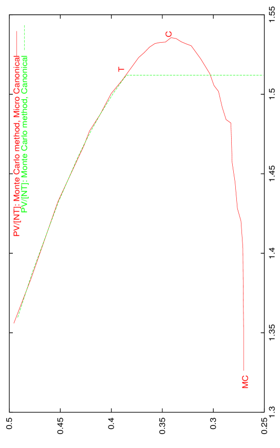
Figure 1: $f(\eta^{R})=PV/[NT]$ as a function of $\eta^{R}$ by Monte Carlo simulations for the microcanonical and canonical ensembles ($N=2000$). Both curves coincide within the statistical error till the point T.

We calculate the saddle point (mean field) for spherical symmetry and we obtain from it the various physical magnitudes (pressure, energy, entropy, free energy, specific heats, compressibilities, speed of sound and particle density). Furthermore, we computed in ref.[2] the determinants of small fluctuations around the saddle point solution for spherical symmetry for the three statistical ensembles.

When any small fluctuation around the saddle point decreases the statistical weight in the functional integral, the saddle point dominates the functional integral and the mean field approach can be valid. In that case, the determinant of small fluctuations is positive. A negative determinant of small fluctuations indicates that some fluctuations around the saddle point are increasing the statistical weight in the functional integral and hence the saddle point does not dominate the partition function. The mean field approach cannot be used when the determinant of small fluctuations is negative. We find analytically in the CE that the determinant of small fluctuations vanishes at the point $\eta_{C}$ = 1.561764 and becames negative at $\eta>\eta_{C}$ [1]. (The point $\eta_{C}$ is indicated $C$ in fig.1). We find that the CE specific heat $c_{V}$ at the point $C$ diverges as [1]:

$$c_{V}\buildrel\eta\uparrow\eta_{C}\over{=}\pm 0.63572\ldots(\eta_{C}-\eta)^{-1/2}-0.19924\ldots+{O}(\sqrt{\eta_{C}-\eta})$$

The (+) sign refers to the positive (first) branch, and the (-) sign to the negative (second) branch (between the points $C$ and $MC$).

However, it must be noticed that the instability point is located at $\eta=\eta_{T}<\eta_{C}$, as shown by both, mean field and Monte Carlo computations. (The point $\eta_{T}$ is indicated $T$ in fig. 1). The onset of instability in the canonical ensemble coincides with the point where the isothermal compressibility diverges. The isothermal compressibility $\kappa_{T}$ is positive from $\eta=0$ till $\eta=\eta_{T}=1.51024\ldots$. At this point $\kappa_{T}$ as well as the specific heat at constant pressure $c_{P}$ diverge and change their signs [1]. Moreover, at this point the speed of sound at the center of the sphere becomes imaginary [2]. Therefore, small density fluctuations will grow exponentially in time instead of exhibiting oscillatory propagation. Such a behaviour leads to the collapse of the gas into a extremely compact object. Monte-Carlo simulations confirm the presence of this instability at $\eta_{T}=1.510\ldots$ in the canonical ensemble and the formation of the collapsed object [1].

The collapse in the Grand Canonical ensemble (GCE) occurs for a smaller value of $\eta=\eta_{GC}=0.49465\ldots$, while in the microcanonical ensemble, the collapse arrives later, in the second sheet, at $\eta=\eta_{MC}=1.25984\ldots$.

We find that the Monte Carlo simulations for self-gravitating gas in the CE and the MCE confirm the stability results obtained from mean field.

The saddle point solution is identical for the three statistical ensembles. This is not the case for the fluctuations around it. The presence of constraints in the CE (on the number of particles) and in the MCE (on the energy and the number of particles) changes the functional integral over the quadratic fluctuations with respect to the GCE.

The saddle point of the partition function turns out to coincide with the hydrostatic treatment of the self-gravitating gas [10, 16] (which is usually known as the ‘isothermal sphere’ in the spherically symmetric case).

We find that the Monte Carlo simulations (describing thermal equilibrium) are much more efficient than the $N$-body simulations integrating Newton’s equations of motion. (Indeed, the integration of Newton’s equations provides much more detailed information than the one needed in thermal equilibrium investigations). Actually, a few hundreds of particles are enough to get quite accurate results in the Monte Carlo simulations (except near the collapse points). Moreover, the Monte Carlo results turns to be in excellent agreement with the mean field calculations up to very small corrections of the order $1/N$. Our Monte Carlo simulations are performed in a cubic geometry. The equilibrium configurations obtained in this manner can thus be called the ‘isothermal cube’.

In summary, the picture we get from our calculations using these three methods show that the self-gravitating gas behaves as a perfect gas for $\eta\to 0,\;1/\xi\to 0$. When $\eta$ and $1/\xi$ grow, the gas becomes denser till it suddenly condenses into a high density object at a critical point GC, C or MC depending upon the statistical ensemble chosen.

$\eta$ is related with the Jeans’ length $d_{J}$ of the gas through $\eta=3\;(L/d_{J})^{2}$. Hence, when $\eta$ goes beyond $\eta_{T}$, the length of the system becomes larger than $d_{J}/\sqrt{\eta_{T}/3}$. The collapse at T in the CE is therefore a manifestation of the Jeans’ instability.

In the MCE, the determinant of fluctuations vanishes at the point MC. The physical states beyond MC are collapsed configurations as shown by the Monte Carlo simulations [see fig. 2]. Actually, the gas collapses in the Monte Carlo simulations slightly before the mean field prediction for the point MC. The phase transition at the microcanonical critical point MC is the so called gravothermal catastrophe [13].

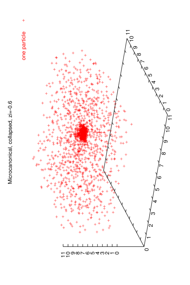
Figure 2: Average particle distribution in the collapsed phase from Monte Carlo simulations with $2000$ particles in the microcanonical ensemble for $\xi=-0.6,\;\eta=0.43,\;pV/[NT]=0.414$.

The gravitational interaction being attractive without lower bound, a short distance cut-off ($A$) must be introduced in order to give a meaning to the partition function. We take the gravitational force between particles as $-G\;m^{2}/r^{2}$ for $r>A$ and zero for $r<A$ where $r$ is the distance between the two particles. We show that the cut-off effects are negligible in the $N=\infty$ limit. That is, once we set $N=\infty$ with fixed $\eta$, all physical quantities are finite in the zero cut-off limit ($A=0$). The cut-off effects are of the order $A^{2}/L^{2}$ and can be safely ignored.

In ref. [1] we expressed all global physical quantities in terms of a single function $f(\eta)$. Besides computing numerically $f(\eta)$ in the mean field approach, we showed that this function obeys a first order non-linear differential equation of first Abel’s type. We obtained analytic results about $f(\eta)$ from the Abel’s equation. $f(\eta)$ exhibits a square-root cut at $\eta_{C}$, the critical point in the CE. The first Riemann sheet is realized both in the CE and the MCE, whereas the second Riemann sheet (where $c_{V}<0$) is only realized in the MCE. $f(\eta)$ has infinitely many branches in the $\eta$ plane but only the first two branches are physically realized. Beyond MC the states described by the mean field saddle point are unstable.

We plot and analyze the equation of state, the energy, the entropy, the free energy, $c_{V}$ and the isothermal compressibility [figs. 6-10]. Most of these physical magnitudes were not previously computed in the literature as functions of $\eta$.

We find analytically the behaviour of $f(\eta)$ near the point $\eta_{C}$ in mean field,

$$f(\eta)\buildrel\eta\uparrow\eta_{C}\over{=}\frac{1}{3}+0.27137\ldots\sqrt{\eta_{C}-\eta}+0.27763\ldots\;(\eta_{C}-\eta)+O\left[(\eta_{C}-\eta)^{3/2}\right]\;.$$

This exhibits a square root branch point singularity at $\eta_{C}$. This shows that the specific heat at constant volume diverges at $\eta_{C}$ as $\left(\eta_{C}-\eta\right)^{-1/2}$ for $\eta\uparrow\eta_{C}$. However, it must be noticed, that the specific heat at constant pressure and the isothermal compressibility both diverge at the point $\eta_{T}$ as $\left(\eta_{T}-\eta\right)^{-1}$. These mean field results apply for $|\eta-\eta_{C}|\ll 1\ll N|\eta-\eta_{C}|$. Fluctuations around mean field can be neglected in such a regime.

The Monte Carlo calculations permit us to obtain $f(\eta)$ in the collapsed phase. Such result cannot be obtained in the mean field approach. The mean field approach only provides information as $f(\eta)$ in the dilute gas phase.

For the self-gravitating gas, we find that the Gibbs free energy $\Phi$ is not equal to $N$ times the chemical potential and that the thermodynamic potential $\Omega$ is not equal to $-PV$ as usual [3]. This is a consequence of the dilute thermodynamic limit $N\to\infty,\;L\to\infty,\;N/L=$fixed.

We computed the determinant of small fluctuations around the saddle point solution for spherical symmetry in all three statistical ensembles. In the spherically symmetric case, the determinant of small fluctuations is written as an infinite product over partial waves. The S and P wave determinants are written in closed form in terms of the saddle solution. The determinants for higher partial waves are computed numerically. All partial wave determinants are positive definite except for the S-wave [2]. The reason why the fluctuations are different in the three ensembles is rather simple. The more contraints are imposed the smaller becomes the space of fluctuations. Therefore, in the grand canonical ensemble (GCE) the system is more free to fluctuate and the phase transition takes place earlier than in the micro-canonical (MCE) and canonical ensembles (CE). For the same reason, the transition takes place earlier in the CE than in the MCE.

The conclusion being that the mean field correctly gives an excellent description of the thermodynamic limit except near the critical points (where the small fluctuations determinant vanishes); the mean field is valid for $N|\eta-\eta_{crit}|\gg 1$. The vicinity of the critical point should be studied in a double scaling limit $N\to\infty,\;\eta\to\eta_{crit}$. Critical exponents are reported in ref. [1] for $\eta\to\eta_{C}$ using the mean field. These mean field results apply for $|\eta-\eta_{C}|\ll 1\ll N|\eta-\eta_{C}|$ with $N\gg 1$. Fluctuations around mean field can be neglected in such a regime.

We computed local properties of the gas in ref.[2]. That is, the local energy density $\epsilon(r)$, local particle density, local pressure and the local speed of sound. Furthermore, we analyze the scaling behaviour of the particle distribution and its fractal (Haussdorf) dimension [2].

The particle distribution $\rho_{V}({\vec{q}})$ proves to be inhomogeneous (except for $\eta\ll 1$) and described by an universal function of $\eta$, the geometry and the ratio ${\vec{r}}={\vec{q}}/R,\;R$ being the radial size. Both Monte Carlo simulations and the Mean Field approach show that the system is inhomogeneous forming a clump of size smaller than the box of volume $V$ [see figs. 3-5].

The particle density in the bulk behaves as $\rho_{V}({\vec{q}})\simeq r^{D-3}$. That is, the mass $M(R)$ enclosed on a region of size $R$ vary approximately as

$$M(R)\simeq C\;R^{D}\;.$$

$D$ slowly decreases from the value $D=3$ for the ideal gas ($\eta=0$) till $D=0.98$ in the extreme limit of the MC point, $D$ takes the value $1.6$ at $\eta_{C}$, [see Table 2]. This indicates the presence of a fractal distribution with Haussdorf dimension $D$.

Our study of the statistical mechanics of a self-gravitating system indicates that gravity provides a dynamical mechanism to produce fractal structures [1, 2, 4].

The average distance between particles monotonically decrease with $\eta$ in the first sheet. The mean field and Monte Carlo are very close in the gaseous phase whereas the Monte Carlo simulations exhibit a spectacular drop in the average particle distance at the clumping transition point T. In the second sheet (only described by the MCE) the average particle distance increases with $\eta$ [2].

We find that the local equation of state is given by

$$p(\vec{r})=T\,\rho_{V}(\vec{r})\;.$$ (1)

We have derived the equation of state for the self-gravitating gas. It is locally the ideal gas equation, but the self-gravitating gas being inhomogeneous, the pressure at the surface of a given volume is not equal to the temperature times the average density of particles in the volume. In particular, for the whole volume: $PV/[NT]=f(\eta)\leq 1$ (the equality holds only for $\eta=0$).

Notice that we have found the local ideal gas equation of state $p(\vec{r})=T\,\rho_{V}(\vec{r})$ for purely gravitational interaction between particles. Therefore, equations of state different from this one, (as often assumed and used in the literature for the self-gravitating gas), necessarily imply the presence of additional non-gravitational forces.

The local energy density $\epsilon(r)$ turns out to be an increasing function of $r$ in the spherically symmetric case. The energy density is always positive on the surface, whereas it is positive at the center for $0\leq\eta<\eta_{3}=1.07783\ldots$, and negative beyond the point $\eta=\eta_{3}=1.07783\ldots$.

The local speed of sound $v_{s}^{2}(r)$ is computed in the mean field approach as a function of the position for spherical symmetry and long wavelengths. $v_{s}^{2}(r)$ diverges at $\eta=\eta_{T}=1.51024\ldots$ in the first Riemann sheet. Just beyond this point $v_{s}^{2}(r)$ is large and negative in the bulk showing the strongly unstable behaviour of the gas for such range of values of $\eta$.

Moreover, we have shown the equivalence between the statistical mechanical treatment in the mean field approach and the hydrostatic description of the self-gravitating gas [10, 16].

The success of the hydrodynamical description depends on the value of the mean free path ($l$) compared with the relevant sizes in the system. $l$ must be $\ll 1$. We compute the ratio $l/a$ (Knudsen number), where $a$ is a length scale that stays fixed for $N\to\infty$ and show that $l/a\sim N^{-2}$. This result ensures the accuracy of the hydrodynamical description for large $N$.

Furthermore, we have computed in ref. [2] several physical magnitudes as functions of $\eta$ and $r$ which were not previously computed in the literature as the speed of sound, the energy density, the average distance between particles and we notice the presence of a Haussdorf dimension in the particle distribution.

The statistical mechanics of a selfgravitating gas formed by particles with different masses is thoroughly investigated in ref.[7] while the selfgravitating gas in the presence of the cosmological constant is thoroughly investigated in refs. [26]. In ref.[27] the Mayer expansion for the selfgravitating gas is investigated in connection with the stability of the gaseous phase.

The variable $\eta^{R}$ appropriate for a spherical symmetry is defined as

$$\eta^{R}\equiv{G\,m^{2}N\over R\;T}=\eta\;\left({4\pi\over 3}\right)^{1/3}=1.61199\ldots\;\eta\;.$$

We use $\eta^{R}$ for the mean field theory calculations with spherical symmetry while $\eta$ is preferred for the Monte Carlo simulations with cubic symmetry.

2 Statistical Mechanics of the Self-Gravitating Gas: the microcanonical and the canonical ensembles

We investigate a gas of $N$ non-relativistic particles with mass $m$ self-interacting through Newtonian gravity. We consider first the particles isolated, that is, a self-gravitating gas in the microcanonical ensemble. We subsequently consider them in thermal equilibrium at temperature $T\equiv\beta^{-1}$. That is, in the canonical ensemble where the system of $N$ particles is not isolated but in contact with a thermal bath at temperature $T$.

We always assume the system being on a cubic box of side $L$ just for simplicity. We consider spherical symmetry for the mean field approach (sec. 4). Please notice that we never use periodic boundary conditions.

At short distances, the particle interaction for the self-gravitating gas in physical situations is not gravitational. Its exact nature depends on the problem under consideration (opacity limit, Van der Waals forces for molecules etc.). We shall just assume a repulsive short distance potential, that is,

$$v_{A}(|{\vec{q}}_{l}-{\vec{q}}_{j}|)=-{1\over|{\vec{q}}_{l}-{\vec{q}}_{j}|_{A}}=\left\{\begin{array}[]{c}-{1\over|{\vec{q}}_{l}-{\vec{q}}_{j}|}\quad\mbox{for}\;|{\vec{q}}_{l}-{\vec{q}}_{j}|\geq A\cr\cr+{1\over A}\quad\mbox{for}\;|{\vec{q}}_{l}-{\vec{q}}_{j}|\leq A\end{array}\right.$$ (2)

where $A<<L$ is the short distance cut-off.

The presence of the repulsive short-distance interaction prevents the collapse (here unphysical) of the self-gravitating gas. In the situations we are interested to describe (interstellar medium, galaxy distributions) the collapse situation is unphysical.

2.1 The microcanonical ensemble

The entropy of the system in can be written as

$$S(E,N)=\log\left\{{1\over N!}\int\ldots\int\prod_{l=1}^{N}{{d^{3}p_{l}\,d^{3}q_{l}}\over{(2\pi)^{3}}}\;\delta\!\left[E-\sum_{l=1}^{N}\;{{p_{l}^{2}}\over{2m}}-U({\vec{q}}_{1},\ldots{\vec{q}}_{N})\right]\right\}$$ (3)

where

$$U({\vec{q}}_{1},\ldots{\vec{q}}_{N})=-G\,m^{2}\sum_{1\leq l<j\leq N}{1\over{|{\vec{q}}_{l}-{\vec{q}}_{j}|_{A}}}$$ (4)

and $G$ is Newton’s gravitational constant.

In order to compute the integrals over the momenta $p_{l},\;(1\leq l\leq N)$, we introduce the variables,

$${\vec{\rho}}_{i}={1\over\sqrt{2m}}\,{\vec{p}}_{i}\;.$$

We can now integrate over the angles in $3N$ dimensions,

$$\int_{-\infty}^{+\infty}\ldots\int_{-\infty}^{+\infty}\prod_{l=1}^{N}\;{d^{3}p_{l}\over{(2\pi)^{3}}}\;\delta\!\left[E-\sum_{l=1}^{N}\;{\vec{\rho}}_{l}^{\,2}-U({\vec{q}}_{1},\ldots{\vec{q}}_{N})\right]$$ (5)

$$= \left({\sqrt{2m}\over 2\pi}\right)^{3N}\;{2\pi^{3N/2}\over\Gamma\left({3N\over 2}\right)}\;\int_{0}^{\infty}\rho^{3N-1}\,d\rho\;\delta\!\left[E-\rho^{2}-U({\vec{q}}_{1},\ldots{\vec{q}}_{N})\right]$$ (7)

$$= \left({m\over 2\pi}\right)^{3N/2}{1\over\Gamma\left({3N\over 2}\right)}\;\left[E-U({\vec{q}}_{1},\ldots{\vec{q}}_{N})\right]^{3N/2-1}\;\theta\left[E-U({\vec{q}}_{1},\ldots{\vec{q}}_{N})\right]$$ (9)

The delta function in the energy thus becomes the constraint of a positive kinetic energy $E-U({\vec{q}}_{1},\ldots{\vec{q}}_{N})>0$. We then get for the entropy,

$$S(E,N)=\log\left\{{\left({m\over 2\pi}\right)^{3N/2}\over N!\,\Gamma\left({3N\over 2}\right)}\,\int_{0}^{L}\ldots\int_{0}^{L}\prod_{l=1}^{N}\;d^{3}q_{l}\;\left[E-U({\vec{q}}_{1},\ldots{\vec{q}}_{N})\right]^{3N/2-1}\theta\left[E-U({\vec{q}}_{1},\ldots{\vec{q}}_{N})\right]\right\}$$ (10)

It is convenient to introduce the dimensionless variables ${\vec{r}}_{l},\;1\leq l\leq N$ making explicit the volume dependence as

$${\vec{q}}_{l} = L\;{\vec{r}}_{l}\quad,\quad{\vec{r}}_{l}=(x_{l},y_{l},z_{l})\;,$$ (11)

$$0 \leq x_{l},y_{l},z_{l}\leq 1\;.$$ (13)

That is, in the new coordinates the gas is inside a cube of unit volume.

The entropy then becomes

$$S(E,N) = \log\left\{{N^{3N-2}\,m^{9N/2-2}\,L^{3N/2+1}\,G^{3N/2-1}\over N!\,\Gamma\left({3N\over 2}\right)\,{(2\pi)}^{3N/2}}\right.$$

$$\left.\int_{0}^{1}\ldots\int_{0}^{1}\prod_{l=1}^{N}\;d^{3}r_{l}\;\left[\xi+{1\over N}u({\vec{r}}_{1},\ldots,{\vec{r}}_{N})\right]^{3N/2-1}\theta\left[\xi+{1\over N}u({\vec{r}}_{1},\ldots,{\vec{r}}_{N})\right]\right\}$$

where we introduced the dimensionless variable $\xi$,

$$\xi\equiv{E\,L\over G\,m^{2}\,N^{2}}$$ (16)

and

$$u({\vec{r}}_{1},\ldots,{\vec{r}}_{N})\equiv{1\over N}\sum_{1\leq l<j\leq N}{1\over{|{\vec{r}}_{l}-{\vec{r}}_{j}|_{a}}}\;.$$ (17)

where $a\equiv A/L\ll 1$.

Let us define the coordinate partition function in the microcanonical ensemble as

$$w(\xi,N)\equiv\int_{0}^{1}\ldots\int_{0}^{1}\prod_{l=1}^{N}\;d^{3}r_{l}\;\left[\xi+{1\over N}u({\vec{r}}_{1},\ldots,{\vec{r}}_{N})\right]^{3N/2-1}\theta\left[\xi+{1\over N}u({\vec{r}}_{1},\ldots,{\vec{r}}_{N})\right]\;.$$ (18)

Therefore,

$$S(E,N)=\log\left[{N^{3N-2}\,m^{9N/2-2}\,L^{3N/2+1}\,G^{3N/2-1}\over N!\,\Gamma\left({3N\over 2}\right)\,{(2\pi)}^{3N/2}}\right]+\log w(\xi,N)\;.$$

We can now compute the thermodynamic quantities, temperature and pressure through the standard thermodynamic relations

$${1\over T}=\left({\partial S\over\partial E}\right)_{V}\quad\mbox{and}\quad p=T\left({\partial S\over\partial V}\right)_{E}\;,$$ (19)

where $V\equiv L^{3}$ stands for the volume of the system and $p$ is the external pressure on the system.

2.2 The canonical ensemble

The partition function in the canonical ensemble can be written as

$${\cal Z}_{C}(N,T)={1\over N!}\int\ldots\int\prod_{l=1}^{N}\;{{d^{3}p_{l}\,d^{3}q_{l}}\over{(2\pi)^{3}}}\;e^{-\beta H_{N}}$$ (20)

where

$$H_{N}=\sum_{l=1}^{N}\;{{p_{l}^{2}}\over{2m}}-G\,m^{2}\sum_{1\leq l<j\leq N}{1\over{|{\vec{q}}_{l}-{\vec{q}}_{j}|_{A}}}$$ (21)

$G$ is Newton’s gravitational constant.

Computing the integrals over the momenta $p_{l},\;(1\leq l\leq N)$

$$\int_{-\infty}^{+\infty}\;{{d^{3}p}\over{(2\pi)^{3}}}\;e^{-{{\beta p^{2}}\over{2m}}}=\left({m\over{2\pi\beta}}\right)^{3/2}$$

yields

$${{\cal Z}_{C}(N,T)={1\over N!}\left({m\over{2\pi\beta}}\right)^{\frac{3N}{2}}\;\int_{0}^{L}\ldots\int_{0}^{L}\prod_{l=1}^{N}d^{3}q_{l}\;\;e^{\beta G\,m^{2}\sum_{1\leq l<j\leq N}{1\over{|{\vec{q}}_{l}-{\vec{q}}_{j}|_{A}}}}}\;.$$ (22)

We make now explicit the volume dependence introducing the variables ${\vec{r}}_{l},\;1\leq l\leq N$ defined in eq.(11). The partition function takes then the form,

$${\cal Z}_{C}(N,T)={1\over N!}\left({mTL^{2}\over{2\pi}}\right)^{\frac{3N}{2}}\;\int_{0}^{1}\ldots\int_{0}^{1}\prod_{l=1}^{N}d^{3}r_{l}\;\;e^{\eta\;u({\vec{r}}_{1},\ldots,{\vec{r}}_{N})}\;,$$ (23)

where we introduced the dimensionless variable $\eta$

$$\eta \equiv {G\,m^{2}N\over L\;T}$$ (24)

and $u({\vec{r}}_{1},\ldots,{\vec{r}}_{N})$ is defined by eq.(17). Recall that

$$U\equiv-{G\,m^{2}N\over L}\;u({\vec{r}}_{1},\ldots,{\vec{r}}_{N})\;,$$ (25)

is the potential energy of the gas.

The free energy takes then the form,

$$F=-T\log{\cal Z}_{C}(N,T)=-NT\log\left[{eV\over N}\left({mT\over 2\pi}\right)^{3/2}\right]-T\;\Phi_{N}(\eta)\;,$$ (26)

where

$$\Phi_{N}(\eta)=\log\int_{0}^{1}\ldots\int_{0}^{1}\prod_{l=1}^{N}d^{3}r_{l}\;\;e^{\eta\;u({\vec{r}}_{1},\ldots,{\vec{r}}_{N})}\;,$$ (27)

The derivative of the function $\Phi_{N}(\eta)$ will be computed by Monte Carlo simulations, mean field methods and, in the weak field limit $\eta<<1$, it will be calculated analytically.

We get for the pressure of the gas,

$$p=-\left({\partial F\over\partial V}\right)_{T}={NT\over V}-{\eta\,T\over 3\,V}\;\Phi_{N}^{\prime}(\eta)\;.$$ (28)

[Here, $V\equiv L^{3}$ stands for the volume of the box and $p$ is the external pressure on the system.]. We see from eq.(27) that $\Phi_{N}(\eta)$ increases with $\eta$ since $u(.)$ is positive. Therefore, the second term in eq.(28) is a negative correction to the perfect gas pressure ${NT\over V}$.

The mean value of the potential energy $U$ can be written from eq.(25) as

$$<U>=-T\eta\;\Phi_{N}^{\prime}(\eta)$$ (29)

Combining eqs.(28) and (29) yields the virial theorem,

$${pV\over NT}=1+{<U>\over 3NT}\quad\mbox{or}\quad{pV\over NT}=\frac{1}{2}+{E\over 3NT}\;,$$ (30)

where we use that the average value of the kinetic energy of the gas is $\frac{3}{2}NT$.

A more explicit form of the equation of state is

$${pV\over NT}=1-{\eta\over 3N}\;\Phi_{N}^{\prime}(\eta)\;,$$ (31)

where

$$\Phi_{N}^{\prime}(\eta) = e^{-\Phi_{N}(\eta)}\;\int_{0}^{1}\ldots\int_{0}^{1}\prod_{l=1}^{N}d^{3}r_{l}\;u({\vec{r}}_{1},\ldots,{\vec{r}}_{N})\;e^{\eta u({\vec{r}}_{1},\ldots,{\vec{r}}_{N})}$$ (32)

$$= \frac{1}{2}(N-1)\;e^{-\Phi_{N}(\eta)}\;\int_{0}^{1}\ldots\int_{0}^{1}\prod_{l=1}^{N}d^{3}r_{l}\;{1\over|{\vec{r}}_{1}-{\vec{r}}_{2}|_{a}}\;e^{\eta u({\vec{r}}_{1},\ldots,{\vec{r}}_{N})}\;.$$ (34)

This formula indicates that $\Phi_{N}^{\prime}(\eta)$ is of order $N$ for large $N$. Monte Carlo simulations as well as analytic calculations for small $\eta$ show that this is indeed the case. In conclusion, we can write the equation of state of the self-gravitating gas as

$${pV\over NT}=f(\eta)\quad,$$ (35)

where the function

$$f(\eta)\equiv 1-{\eta\over 3N}\;\Phi_{N}^{\prime}(\eta)\;,$$

is independent of $N$ for large $N$ and fixed $\eta$. [In practice, Monte Carlo simulations show that $f(\eta)$ is independent of $N$ for $N>100$].

We get in addition,

$$<U>=-3NT\;[1-f(\eta)]\;.$$ (36)

In the dilute limit, $\eta\to 0$ and we find the perfect gas value

$$f(0)=1\;.$$

Equating eqs.(31) and (35) yields,

$$\Phi_{N}(\eta)=3N\,\int_{0}^{\eta}dx\,{1-f(x)\over x}\;.$$

Relevant thermodynamic quantities can be expressed in terms of the function $f(\eta)$. We find for the free energy from eq.(26),

$$F=F_{0}-3NT\;\int_{0}^{\eta}dx\;{1-f(x)\over x}\;.$$ (37)

where

$$F_{0}=-NT\log\left[{eV\over N}\left({mT\over 2\pi}\right)^{3/2}\right]$$ (38)

is the free energy for an ideal gas.

We find for the total energy $E$, chemical potential $\mu$ and entropy $S$ the following expressions,

$$E = 3NT\left[f(\eta)-\frac{1}{2}\right]\;,$$ (39)

$$\mu = \left({\partial F\over\partial N}\right)_{T,V}=-T\log\left[{V\over N}\left({mT\over 2\pi}\right)^{3/2}\right]-3T[1-f(\eta)]-3T\;\int_{0}^{\eta}dx\,{1-f(x)\over x}\;,$$ (41)

$$S = -\left({\partial F\over\partial T}\right)_{V}$$ (43)

$$= S_{0}+3N\left[\int_{0}^{\eta}dx\,{1-f(x)\over x}+f(\eta)-1\right]\;,$$ (45)

where

$$S_{0}=-{F_{0}\over T}+\frac{3}{2}N\;.$$

is the entropy of the ideal gas.

Notice that here the Gibbs free energy

$$\Phi=F+pV=F_{0}+NT\left[f(\eta)-3\,\int_{0}^{\eta}dx\,{1-f(x)\over x}\right]\;,$$ (46)

is not proportional to the chemical potential. That is, here $\Phi\neq\mu\,N$ and we have instead,

$$\Phi-\mu\,N=2NT\left[1-f(\eta)\right]\;.$$ (47)

This relationship differs from the customary one (see [3]) due to the fact that the dilute scaling relation $N\sim L$ holds here instead of the usual one $N\sim L^{3}$. The usual relationship is only recovered in the ideal gas limit $\eta=0$.

The specific heat at constant volume takes the form[3],

$$c_{V} = {T\over N}\left({\partial S\over\partial T}\right)_{V}=3\left[f(\eta)-\eta\;f^{\prime}(\eta)-\frac{1}{2}\right]\;.$$ (48)

where we used eq.(43). This quantity is also related to the fluctuations of the potential energy $(\Delta U)^{2}$ and it is positive defined in the canonical ensemble,

$$c_{V}=\frac{3}{2}+(\Delta U)^{2}\;.$$ (49)

Here,

$$(\Delta U)^{2}\equiv{{<U^{2}>-<U>^{2}}\over N\;T^{2}}=3\left[f(\eta)-\eta\;f^{\prime}(\eta)-1\right]\;.$$ (50)

The specific heat at constant pressure is given by [3]

$$c_{P}=c_{V}-{T\over N}{{\left({\partial p\over\partial T}\right)^{2}_{V}}\over{\left({\partial p\over\partial V}\right)_{T}}}\;.$$ (51)

and then,

$$c_{P} = c_{V}+{\left[f(\eta)-\eta f^{\prime}(\eta)\right]^{2}\over f(\eta)+\frac{1}{3}\eta f^{\prime}(\eta)}$$ (52)

$$= -\frac{3}{2}+{{4\,f(\eta)\left[f(\eta)-\eta f^{\prime}(\eta)\right]}\over{f(\eta)+\frac{1}{3}\eta f^{\prime}(\eta)}}\;.$$ (54)

The isothermal ($K_{T}$) and adiabatic ($K_{S}$) compressibilities take the form

$$K_{T} = -{1\over V}\left({\partial V\over\partial p}\right)_{T}={V\over N\,T}{1\over{f(\eta)+\frac{1}{3}\eta f^{\prime}(\eta)}}\;,$$ (55)

$$K_{S} = -{1\over V}\left({\partial V\over\partial p}\right)_{S}={c_{V}\over c_{P}}\;K_{T}\;.$$ (57)

It is then convenient to introduce the compressibilities

$$\kappa_{T}\equiv{NT\over V}\,K_{T}={1\over{f(\eta)+\frac{1}{3}\eta f^{\prime}(\eta)}}\quad\mbox{and}\quad\kappa_{S}\equiv{NT\over V}\,K_{S}={c_{V}\over c_{P}}\;\kappa_{T}\;,$$ (58)

which are both of order one (intensive) in the $N,\;L\to\infty$ limit with $N/L$ fixed.

The speed of sound $v_{s}$ can be written as [17]

$$v_{s}^{2}=-{{c_{P}\;V^{2}}\over{c_{V}\;N}}\left({\partial p\over\partial V}\right)_{T}={V^{2}\over N}\left[{T\over N\,c_{V}}\left({\partial p\over\partial T}\right)^{2}_{V}-\left({\partial p\over\partial V}\right)_{T}\right]\;.$$ (59)

where we used eq.(51) in the last step. Therefore,

$${v_{s}^{2}\over T}={\left[f(\eta)-\eta f^{\prime}(\eta)\right]^{2}\over 3\left[f(\eta)-\eta f^{\prime}(\eta)-\frac{1}{2}\right]}+f(\eta)+\frac{1}{3}\eta f^{\prime}(\eta)\;.$$ (60)

The pressure $p$ used in this calculation corresponds to the pressure on the surface of the system. Hence, this is the speed of sound on the surface of the system, this is different from the speed of sound inside the volume since the ground state is inhomogeneous. We compute the speed of sound as a function of the point in [2].

We see that the large $N$ limit of the self-gravitating gas is special. Energy, free energy and entropy are extensive magnitudes in the sense that they are proportional to the number of particles $N$ (for fixed $\eta$). They all depend on the variable $\eta={G\,m^{2}N\over L\;T}$ which is to be kept fixed for the thermodynamic limit ($N\to\infty$ and $V\to\infty$) to exist. Notice that $\eta$ contains the ratio $N/L=N\;V^{-1/3}$ which must be considered here an intensive variable. Here, the presence of long-range gravitational situations calls for this new intensive variable in the thermodynamic limit.

In addition, all physical magnitudes can be expressed in terms of a single function of one variable: $f(\eta)$.

3 Monte Carlo Simulations

The Metropolis algorithm[18] was applied for the first time to the self-gravitating gas in ref.[1]. We computed in this way the pressure, the energy, the average density, the potential energy fluctuations, the average particle distance and the average squared particle distance as functions of $\eta$ for the self-gravitating gas in a cube of size $L$ in the canonical ensemble at temperature $T$[1].

We implemented the Metropolis algorithm in the following way. We start from a random distribution of $N$ particles in the chosen volume. We update such configuration choosing a particle at random and changing at random its position. We then compare the energies of the former and the new configurations. We use the standard Metropolis test to choose between the new and the former configurations. The energy of the configurations are calculated performing the exact sums as in eq.(17). We use as statistical weight for the Metropolis algorithm in the canonical ensemble,

$$e^{\eta\;u({\vec{r}}_{1},\ldots,{\vec{r}}_{N})}\;,$$

which appears in the coordinate partition function eq.(27). The number of particles $N$ went up to $2000$.

We introduced a small short distance cutoff $A=10^{-4}L-10^{-8}L$ in the attractive Newton’s potential according to eq.(2). All results in the gaseous phase were insensitive to the cutoff value. The partition function calculation turns to be much less sensible to the short distance singularities of the gravitational force than Newton’s equations of motion for $N$ particles. That is, solving the classical dynamics for $N$ particles interacting through gravitational forces as well as solving the Boltzman equation including the $N$-body gravitational interaction requires sophisticated algorithms to avoid excessively long computer times. As is clear, solving the $N$-body classical evolution or the kinetic equations provides the time-dependent dynamics and out of thermal equilibrium effects which are out of the scope of our approach.

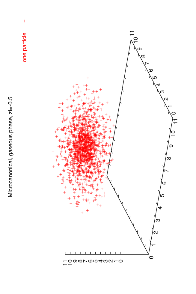
Figure 3: Average particle distribution in the gaseous phase from Monte Carlo simulations with $2000$ particles in the microcanonical ensemble for $\xi=-0.5,\;\eta=1.38,\;pV/[NT]=0.277$.

In the CE, two different phases show up: for $\eta<\eta_{T}$ we have a non-perfect gas and for $\eta>\eta_{T}$ it is a condensed system with negative pressure. The transition between the two phases is very sharp. This phase transition is associated with the Jeans instability.

A negative pressure indicates that the free energy grows for increasing volume at constant temperature [see eq.(28)]. Therefore, the system wants to contract sucking on the walls.

We plot in fig. 1 $f(\eta)=pV/[NT]$ as function of $\eta$. $pV/[NT]$ monotonically decreases with $\eta$.

We find an excellent agreement between the the Monte Carlo and the mean field results for $pV/[NT]$ in the gaseous phase plotted in fig. 6. This excellent agreement appears for $N$ as low as $500$.

In the Monte Carlo simulations the phase transition to the condensed phase happens for $\eta=\eta_{T}$ slightly below $\eta_{C}$. For $N=2000$ we find $\eta_{T}\sim 1.515$. For $\eta_{T}<\eta<\eta_{C}$, the gaseous phase only exists as a short lived metastable state as seen in our simulations.

The average distance between particles $<r>$ and the average squared distance between particles $<r^{2}>$ monotonically decrease with $\eta$. When the gas collapses at $\eta_{T}\;,<r>$ and $<r^{2}>$ exhibit a sharp decrease.

The values of $pV/[NT],\;<r>$ and $<r^{2}>$ in the condensed phase are independent of the cutoff for $a<10^{-5}$. The Monte Carlo results in this condensed phase can be approximated for $\eta>2$ as

$${pV\over NT}=f(\eta)\simeq 1-K\;\eta\quad,\quad<r>\simeq 0.016\;.$$ (61)

where $K\simeq 14$.

Since $f(\eta)$ has a jump at the transition, the Gibbs free energy $\Phi$ is discontinuous and we have a phase transition of the zeroth order. We find from eq.(46)

$${\Phi(\mbox{collapse})-\Phi(\eta_{T})\over N\,T}=f(\mbox{collapse})-f(\eta_{T})\simeq-21<0\;.$$ (62)

We can easily compute the latent heat of the transition per particle ($q$) using the fact that the volume $V$ stays constant. Hence, $q=\Delta E/N$ and we obtain from eq.(39)

$${q\over T}={E(\mbox{collapse})-E(\eta_{T})\over N\,T}=3\;\left[f(\mbox{collapse})-f(\eta_{T})\right]\simeq 2-3\,K\;\eta_{T}\simeq-62<0\;.$$ (63)

This phase transition is different from the usual phase transitions since the two phases cannot coexist in equilibrium as their pressures are different.

Eq.(61) can be understood from the general treatment in sec. III as follows. We have from eqs.(31)-(32)

$$f(\eta)=1-{\eta\over 3}<{1\over r}>\;.$$ (64)

The Monte Carlo results indicate that $<{1\over r}>\simeq 42$ is approximately constant in the collapsed region as well as $<r>$ and $<r^{2}>$. Eq.(61) thus follows from eq.(64) using such value of $<{1\over r}>$.

The behaviour of $pV/[NT]$ near $\eta_{C}$ in the gaseous phase can be well reproduced by

$${pV\over NT}=f(\eta)\;\;{\buildrel\eta\uparrow\eta_{C}\over{=}}\;f_{C}+A\;\sqrt{\eta_{C}-\eta}$$ (65)

where $f_{C}\simeq 0.316,\;A\simeq 0.414$ and $\eta_{C}\simeq 1.540$.

In addition, the behaviour of $(\Delta U)^{2}$ in the same region is well reproduced by

$$(\Delta U)^{2}\;\;{\buildrel\eta\uparrow\eta_{C}\over{=}}\;\;C+{D\over\sqrt{\eta_{C}-\eta}}$$ (66)

with $C\simeq-1.64$ and $D\simeq 0.901$. [Notice that for finite $N,\;(\Delta U)^{2}$ will be finite albeit very large at the phase transition]. Eq.(50) relating $f(\eta)$ and $(\Delta U)^{2}$ is satisfied with reasonable approximation.

We thus find a critical region just below $\eta_{C}$ where the energy fluctuations tend to infinity as $\eta\uparrow\eta_{C}$.

The point $\eta_{T}$ where the phase transition actually takes place in the Monte Carlo simulations is at $\eta_{T}\simeq 1.51<\eta_{C}$. This value for $\eta_{T}$ is numerically close to the point where the isothermal compressibility $\kappa_{T}$ diverges and becomes negative. As stressed in ref.[1, 2] these two points actually coincide. The collapse observed in the Monte Carlo simulations corresponds to the singularity of $\kappa_{T}$ where, in addition, the speed of sound at the origin becomes imaginary[1, 2].

Since Monte Carlo simulations are like real experiments, we conclude that the gaseous phase extends from $\eta=0$ till $\eta=\eta_{T}$ in the CE and not till $\eta=\eta_{C}$. Notice that in the literature based on the hydrostatic description of the self-gravitating gas [10, 14, 15, 16], only the instability at $\eta=\eta_{C}$ is discussed whereas the singularities at $\eta=\eta_{T}$ are not considered.

We then performed Monte Carlo calculations in the microcanonical ensemble where the coordinate partition function is given by eq.(18). We thus used

$$\left[\xi+{1\over N}\,u({\vec{r}}_{1},\ldots,{\vec{r}}_{N})\right]^{3N/2-1}\theta\left[\xi+{1\over N}\,u({\vec{r}}_{1},\ldots,{\vec{r}}_{N})\right]\;,$$

as the statistical weight for the Metropolis algorithm.

The MCE and CE Monte Carlo results coincide up to the statistical error for $0<\eta<\eta_{T}$, that is for $\infty>\xi>\xi_{T}\simeq-0.19$. In the MCE the gas does not clump at $\eta=\eta_{C}$ (point $C$ in fig. 1) and the specific heat becomes negative between the points $C$ and $MC$. In the MCE the gas does clump at $\xi\simeq-0.52\;,\;\eta^{T}_{MC}\simeq 1.33$ (point $MC$ in fig. 1) increasing both its temperature and pressure discontinuously. We find from the Monte Carlo data that the temperature increases by a factor $2.4$ whereas the pressure increases by a factor $3.6$ when the gas clumps. The transition point $\eta^{T}_{MC}$ in the Monte Carlo simulations is slightly to the right of the critical point $\eta_{MC}$ predicted by mean field theory. The mean field yields for the sphere $\eta_{MC}=1.2598\ldots$.

As is clear, the domain between $C$ and $MC$ cannot be reached in the CE since $c_{V}>0$ in the CE as shown by eq.(49).

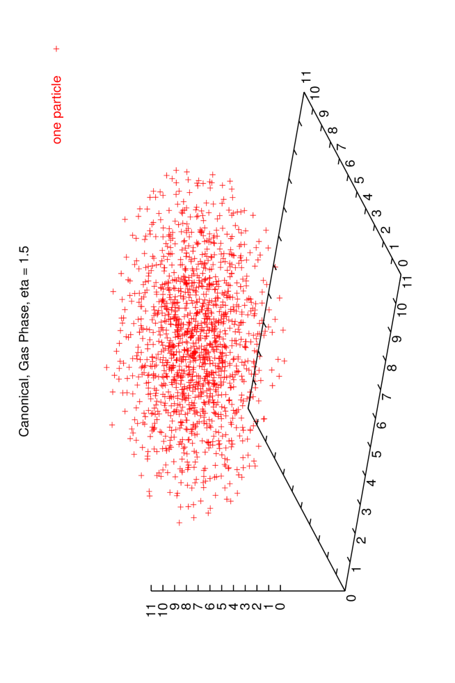
Figure 4: Average particle distribution in the gaseous phase from Monte Carlo simulations in the canonical ensemble for $\eta=1.5$ and $N=2000$

We find an excellent agreement between the Monte Carlo and Mean Field (MF) results (both in the MCE and CE). (This happens although the geometry for the MC calculation is cubic while it is spherical for the MF). The points where the collapse phase transition occurs ($\eta_{T}$ and $\eta^{T}_{MC}$) slowly increase with the number of particles $N$.

We verified that the Monte Carlo results in the gaseous phase ($\eta<\eta_{T}$) are cutoff independent for $10^{-3}\geq a\geq 10^{-7}$.

As for the CE, the Gibbs free energy is discontinuous at the transition in the MCE. The transition is then of the zeroth order. We find from eq.(46)

$${\Phi(\mbox{collapse})-\Phi(\eta_{T})\over N\,T_{gas}}={T_{coll}\over T_{gas}}\,f(\mbox{collapse})-f(\eta_{T})\simeq 0.7>0\;.$$

where we used the numerical values from the Monte Carlo simulations. Notice that the Gibbs free energy increases at the MC transition whereas it decreases at the C transition [see eq.(62)].

Here again the two phases cannot coexist in equilibrium since their pressures and temperatures are different.

We display in figs. 3-2 the average particle distribution from Monte Carlo simulations with $2000$ particles in the microcanonical ensemble at both sides of the gravothermal catastrophe, i. e. $\eta=\eta_{MC}$. Fig. 3 corresponds to the gaseous phase and fig. 2 to the collapsed phase. The inhomogeneous particle distribution is clear in fig. 3 whereas fig. 2 shows a dense collapsed core surrounded by a halo of particles.

The different nature of the collapse in the CE and in the MCE can be explained using the virial theorem [see eq.(30)]

$${p\,V\over N\,T}=1+{U\over N\,T}\;.$$

When the gas collapses in the CE the particles get very close and $U$ becomes large and negative while $T$ is fixed. Therefore, $p\,V\over N\,T$ may become large and negative as it does.

We can write the virial theorem also as,

$$p\,V-\frac{1}{2}\,NT=\frac{1}{3}\,E\;.$$

When the gas is near the point MC, $E<0$ is fixed and we have $T>0$. Therefore, $p\,V\over N\,T$ as well as $U=E-3\,N\,T/2$ cannot become large and negative as in the CE collapse. This prevents the distance between the particles to decrease. Actually, the Monte Carlo simulations show that $<r>$ increases by $18\%$ when the gas collapses in the MCE.

Figs. 4 and 5 depict the average particle distribution from Monte Carlo simulations with $2000$ particles in the canonical ensemble at both sides of the collapse critical point, i. e. $\eta=\eta_{C}$. Fig. 4 corresponds to the gaseous phase and fig. 5 to the collapsed phase. The inhomogeneous particle distribution is clear in fig. 4 whereas fig. 5 shows a dense collapsed core surrounded by a very little halo of particles.

Figure 5: Average particle distribution in the collapsed phase from Monte Carlo simulations with $2000$ particles in the canonical ensemble for $\eta=1.53,\;pV/[NT]=-14.44$.

Notice that the collapsed phases are of different nature in the CE and MCE. The core is much tighter and the halo much smaller in the CE than in the MCE.

Figs. 3 and 5 depict the average particle distribution for the gaseous phase in the MCE and the CE, respectively. In this phase, the MC simulations give identical descriptions for large $N$ in both ensembles. [This important point will be further demostrated in sec. VI by functional integral methods]. The average configurations in figs. 3 and 5 describe a self-gravitating gas in thermal equilibrium within a cube. We may call it the isothermal cube by analogy with the well known isothermal sphere[11]-[16].

4 Mean Field Approach

Both in the microcanonical and the canonical ensembles the coordinate partition functions are given by $3N$-uple integrals [eqs.(18) and (27), respectively]. In the $N\to\infty$ limit both $3N$-uple integrals can be recasted as functional integrals over the continuous particle density as shown in refs.[1, 2]. We present here the mean field approach in the canonical ensemble. The mean field approach for the microcanonical and grand canonical ensembles can be find in refs.[1, 2].

The coordinate partition function $e^{\Phi_{N}(\eta)}$ given by eq.(27) can be recasted as a functional integral in the thermodynamic limit.

$$e^{\Phi_{N}(\eta)} \buildrel N>>1\over{=} \int\int D\rho\;d{\hat{a}}\;e^{-Ns_{C}[\rho(.),\hat{a},\eta]}$$ (67)

$$s_{C}[\rho(.),\hat{a},\eta] = -{\eta\over 2}\int{d^{3}x\;d^{3}y\over|{\vec{x}}-{\vec{y}}|}\;\rho({\vec{x}})\;\rho({\vec{y}})+\int d^{3}x\;\rho({\vec{x}})\;\log\rho({\vec{x}})-i{\hat{a}}\left(\int d^{3}x\,\rho({\vec{x}})-1\right)\;.$$

where we used the coordinates $\vec{x}$ in the unit volume. The first term is the potential energy, the second term is the functional integration measure for this case (see appendix A). Here $N\;\rho({\vec{x}})$ stands for the density of particles.

The integration over $\hat{a}$ enforces the number of particles to be exactly $N$:

$$\int d^{3}x\;\rho({\vec{x}})=1$$ (69)

That is, in the coordinates $\vec{q}$ (running from $0$ to $L$), the density of particles is

$${N\over L^{3}}\;\rho({\vec{q}})\quad{\rm with}\quad\int d^{3}q\;{N\over L^{3}}\;\rho({\vec{q}})=N\;.$$

The functional integral in eq.(67) is dominated for large $N$ by the extrema of the ‘effective action’ $s_{C}[\rho(.),\hat{a},\eta]$, that is, the solutions of the stationary point equation

$$\log\rho_{s}({\vec{x}})-\eta\int{d^{3}y\;\rho_{s}({\vec{y}})\over|{\vec{x}}-{\vec{y}}|}=a_{s}\;,$$ (70)

$a=i{\hat{a}}$ is a Lagrange multiplier enforcing the constraint (69).

Applying the Laplacian and setting $\phi({\vec{x}})\equiv\log\rho_{s}({\vec{x}})$ yields,

$$\nabla^{2}\phi({\vec{x}})+4\pi\eta\;e^{\phi({\vec{x}})}=0\;,$$ (71)

This equation is scale covariant [5]. That is, if $\phi({\vec{x}})$ is a solution of eq.(71), then

$$\phi_{\lambda}({\vec{x}})\equiv\phi(\lambda{\vec{x}})+\log\lambda^{2}$$ (72)

where $\lambda$ is an arbitrary constant is also a solution of eq.(71). For spherically symmetric solutions this property can be found in ref.[9].

Integrating eq.(71) over the unit volume and using the constraint (69) yields

$$\int{\vec{\nabla}}\phi({\vec{x}})\cdot d{\vec{s}}=-4\pi\eta$$ (73)

where the surface integral is over the boundary of the unit volume.

In the mean field approximation we only keep the dominant order for large $N$. Therefore, only the exponent at the saddle point accounts and according to eq.(26) we find for the free energy

$$F = F_{0}+N\,T\,s(\eta)+{\cal O}(N^{0})$$ (74)

$${pV\over NT} = 1+{\eta\over 3}{ds\over d\eta}+{\cal O}(N^{-1})$$ (76)

Hence, in the mean field approximation, the function $f(\eta)$ is given by

$$f_{MF}(\eta)\equiv 1+{\eta\over 3}{ds\over d\eta}\;,$$ (77)

From eq.(67) we can compute $s(\eta)$ in terms of the saddle point solution as follows

$$s(\eta)\equiv s_{C}[\rho_{s}(.),a_{s},\eta]=-{\eta\over 2}\int{d^{3}x\;d^{3}y\over|{\vec{x}}-{\vec{y}}|}\;\rho_{s}({\vec{x}})\;\rho_{s}({\vec{y}})+\int d^{3}x\;\rho_{s}({\vec{x}})\;\log\rho_{s}({\vec{x}})\;.$$ (78)

Using eq.(70) we find the equivalent expression,

$$s(\eta)={a_{s}\over 2}+\frac{1}{2}\int\phi({\vec{x}})\;e^{\phi({\vec{x}})}\;d^{3}x\;.$$ (79)

5 Mean Field Results

Let us summarize here the main results of ref. [1] in the mean field approach for spherical symmetry.

The saddle point is given by

$$\phi(r)=\log\rho(r)=\log\left({\lambda^{2}\over 4\,\pi\,\eta^{R}}\right)+\chi(\lambda\,r)\;.$$ (80)

Here $\rho(r)$ is the particle density and $\chi(\lambda)$ obeys the equation

$$\chi^{\prime\prime}(\lambda)+{2\over\lambda}\,\chi^{\prime}(\lambda)+e^{\chi(\lambda)}=0\quad,\quad\chi^{\prime}(0)=0\quad,\quad\chi(0)=0\ ;.$$ (81)

$\chi(x)$ is independent of $\eta^{R}$, and $\lambda$ is related to $\eta^{R}$ through

$$\lambda\;\chi^{\prime}(\lambda)=-\eta^{R}\;.$$ (82)

We have in addition,

$$\phi(1)=\log\left[{3\,f_{MF}(\eta^{R})\over 4\,\pi}\right]\quad,\quad\rho(1)={3\over 4\,\pi}\;f_{MF}(\eta^{R})\;.$$ (83)

Figure 6: $f_{MF}(\eta^{R})=PV/[NT]$ as a function of $\eta^{R}$ in the MF approximation [eq.(85)]. $f_{MF}(\eta^{R})$ has a square root branch point at $\eta^{R}_{C}$. The points GC, C and MC indicate the transition to the collapsed phase for each ensemble (grand canonical, canonical and microcanonical, respectively): $\eta^{R}_{GC}=0.797375\ldots,\;\eta^{R}_{C}=2.517551\ldots,\;\eta^{R}_{MC}=2.03085\ldots$ (notice that $\eta^{R}_{MC}$ is in the second Riemann sheet). Since $E/[3NT]=f_{MF}(\eta^{R})-\frac{1}{2}$, this plot also shows the energy per particle as a function of $\eta^{R}$. Furthermore, the particle density at the surface is proportional to $f_{MF}(\eta^{R})$ [see eq.(83)].

Figure 7: The entropy per particle minus the ideal gas value as a function of $\eta^{R}$ in the MF approximation [eq.(89)].

Figure 8: ${F-F_{0}\over NT}$ as a function of $\eta$ in the MF approximation [eq.(89)].

where

$$f_{MF}(\eta^{R})={\lambda^{2}\over 3\,\eta^{R}}\;e^{\chi(\lambda)}\quad,$$ (84)

The function $f_{MF}(\eta^{R})$ obeys the Abel equation,

$$\eta^{R}(3f_{MF}-1)f^{\prime}_{MF}(\eta^{R})+(3f_{MF}-3+\eta^{R})f_{MF}=0\;.$$ (85)

For $\eta^{R}=0$ it follows from eq.(85) that

$$f_{MF}(0)=1\;.$$ (86)

Integrating eq.(85) with respect to $\eta^{R}$ yields,

$$3\int_{0}^{\eta^{R}}{dx\over x}[1-f_{MF}(x)]=3[f_{MF}(\eta^{R})-1]+\eta^{R}-\log f_{MF}(\eta^{R})$$

We derive in [1] the properties of the function $f_{MF}(\eta^{R})$ from the differential equation (85). One easily obtains for small $\eta^{R}$ (dilute regime),

$$f_{MF}(\eta^{R})=1-\frac{\eta^{R}}{5}-\frac{(\eta^{R})^{2}}{175}+{\cal O}([\eta^{R}]^{3})\;.$$

These terms exactly coincide with the perturbative calculation in the dilute regime for spherical symmetry [1].

We plot in fig. 6 $f_{MF}(\eta^{R})$ as a function of $\eta^{R}$ obtained by solving eq.(85) by the Runge-Kutta method. We see that $f_{MF}(\eta^{R})$ is a monotonically decreasing function of $\eta^{R}$ for $0<\eta^{R}<\eta^{R}_{C}$. At the point $\eta^{R}=\eta^{R}_{C}$, the derivative $f_{MF}^{\prime}(\eta^{R})$ takes the value $-\infty$. It then follows from eq.(85) that

$$f_{MF}(\eta^{R}_{C})=\frac{1}{3}\;.$$

At the point $\eta^{R}_{C}$ the series expansion for $f_{MF}(\eta^{R})$ in powers of $\eta^{R}$ diverges. Both, from the ratio test on its coefficients and from the Runge-Kutta solution, we find that

$$\eta^{R}_{C}=2.517551\ldots$$ (87)

From eq.(85) we find that $f_{MF}(\eta^{R})-\frac{1}{3}$ has a square root behaviour around $\eta^{R}=\eta^{R}_{C}$:

$$f_{MF}(\eta^{R})\buildrel\eta^{R}\uparrow\eta^{R}_{C}\over{=}\frac{1}{3}+\sqrt{2(\eta^{R}_{C}-2)\over 9\,\eta^{R}_{C}}\;\sqrt{\eta^{R}_{C}-\eta^{R}}+{2\,(\eta^{R}_{C}-1)\over 7\,\eta^{R}_{C}}\;(\eta^{R}_{C}-\eta^{R})+{\cal O}\left[(\eta^{R}_{C}-\eta^{R})^{3/2}\right]$$

Inserting the numerical value (87) for $\eta^{R}_{C}$ yields,

$$f_{MF}(\eta^{R})\buildrel\eta^{R}\uparrow\eta^{R}_{C}\over{=}\frac{1}{3}+0.213738\ldots\sqrt{\eta^{R}_{C}-\eta^{R}}+0.172225\ldots\;(\eta^{R}_{C}-\eta^{R})+{\cal O}\left[(\eta^{R}_{C}-\eta^{R})^{3/2}\right]$$ (88)

We see that $f_{MF}(\eta^{R})$ becomes complex for $\eta^{R}>\eta^{R}_{C}$. Recall that in the Monte Carlo simulations the gas phase collapses at the point $\eta^{R}_{T}<\eta^{R}_{C}$. $f_{MF}(\eta^{R})$ is a multivalued function of $\eta^{R}$ as well as all physical magnitudes [see eq.(89)].

The points GC, C and MC correspond to the collapse phase transition in the grand canonical, canonical and microcanonical ensembles, respectively. Their positions are determined by the breakdown of the mean field approximation through the analysis of the small fluctuations.

As noticed before, the CE only describes the region between the ideal gas point, $\eta^{R}=0$ and $C$ in fig. 1. The MCE goes beyond the point $C$ (till the point $MC$) with the physical magnitudes described by the second sheet of the square root in eqs.(88) (minus sign). We have near $C$ between $C$ and $MC$,

$$f_{MF}(\eta^{R})\buildrel\eta^{R}\uparrow\eta^{R}_{C}\over{=}\frac{1}{3}-0.213738\ldots\sqrt{\eta^{R}_{C}-\eta^{R}}+0.172225\ldots\;(\eta^{R}_{C}-\eta^{R})+{\cal O}\;\left[(\eta^{R}_{C}-\eta^{R})^{3/2}\right]$$

The function $f_{MF}(\eta^{R})$ takes its absolute minimum at $\eta^{R}=\eta^{R}_{min}=2.20731\ldots$ in the second sheet where $f_{MF}(\eta^{R}_{min})=0.264230\ldots$. Since $f_{MF}(\eta^{R})<\frac{1}{2}$ implies that the total energy is negative [see eq.(89)], the gas is in a ‘bounded state’ for $\eta^{R}$ beyond $\eta^{R}_{2}=2.18348\ldots$ in the first sheet.

Figure 9: $(c_{V})_{MF}$ as a function of $\eta^{R}$ from mean field eq.(96). Notice that $(c_{V})_{MF}$ diverges at the point C, that is for $\eta^{R}_{C}=2.517551\ldots$

For the main physical magnitudes in the mean field approach, [that is, from the above saddle point and neglecting the fluctuations around it] we find:

$${pV\over NT} = f_{MF}(\eta^{R})$$ (89)

$${F-F_{0}\over NT} = 3[1-f_{MF}(\eta^{R})]-\eta^{R}+\log f_{MF}(\eta^{R})$$ (91)

$${S-S_{0}\over N} = 6[f_{MF}(\eta^{R})-1]+\eta^{R}-\log f_{MF}(\eta^{R})$$ (93)

$${E\over NT} = 3[f_{MF}(\eta^{R})-\frac{1}{2}]\;,$$

We find for the speed of sound squared at the surface

$${v_{s}^{2}\over T}={f_{MF}(\eta^{R})\over 3}\,\left[4+{3\,f_{MF}(\eta^{R})+\frac{\eta^{R}}{2}-2\over 6\,f_{MF}^{2}(\eta^{R})+\left(\eta^{R}-\frac{11}{2}\right)f_{MF}(\eta^{R})+\frac{1}{2}}\right]\;,$$ (95)

The specific heat at constant volume takes the form

$$(c_{V})_{MF}=6\,f_{MF}(\eta^{R})-\frac{7}{2}+\eta^{R}+{\eta^{R}-2\over 3\,\,f_{MF}(\eta^{R})-1}\;.$$ (96)

We plot in Fig. 9 eq.(96) for $(c_{V})_{MF}$ as a function of $\eta$. We see that $(c_{V})_{MF}$ increases with $\eta$ till it tends to $+\infty$ for $\eta^{R}\uparrow\eta^{R}_{C}$. It has a square-root branch point at the point C. In the stretch C-MC (only physically realized in the microcanonical ensemble), $(c_{V})_{MF}$ becomes negative. We shall not discuss here the peculiar properties of systems with negative $C_{V}$ as they can be find in refs.[12, 13, 16]

From eqs.(88) and (96) we obtain the following behaviour near the point $C$ in the positive (first) branch

$$(c_{V})_{MF} \buildrel\eta^{R}\uparrow\eta^{R}_{C}\over{=} 0.80714\ldots(\eta^{R}_{C}-\eta^{R})^{-1/2}-0.19924\ldots+{\cal O}(\sqrt{\eta^{R}_{C}-\eta^{R}})$$ (97)

and between $C$ and $MC$ in the negative (second) branch

$$(c_{V})_{MF} \buildrel\eta^{R}\uparrow\eta^{R}_{C}\over{=} -0.80714\ldots(\eta^{R}_{C}-\eta^{R})^{-1/2}-0.19924\ldots+{\cal O}(\sqrt{\eta^{R}_{C}-\eta^{R}})$$

Finally, $(c_{V})_{MF}$ vanishes at the point MC $\eta^{R}_{MC}=2.03085\ldots$.

The isothermal compressibility in mean field follows from eqs.(55) and (85)

$$(\kappa_{T})_{MF}={3\over 2f_{MF}(\eta^{R})}\,\left[1+{\eta^{R}-2\over 6f_{MF}(\eta^{R})-\eta^{R}}\right]\;.$$ (98)

We plot $(\kappa_{T})_{MF}$ in fig. 10. We see that $(\kappa_{T})_{MF}$ is positive for $0\leq\eta^{R}<\eta^{R}_{T}=2.43450\ldots$ where $(\kappa_{T})_{MF}$ diverges. The point $\eta^{R}_{T}$ is defined by the equation

$$6f_{MF}(\eta^{R}_{T})-\eta^{R}_{T}=0\;.$$ (99)

We find from eqs.(85) and (99) that

$$f_{MF}^{\prime}(\eta^{R}_{T})=-\frac{1}{2}$$ (100)

$(\kappa_{T})_{MF}$ diverges for $\eta^{R}\simeq\eta^{R}_{T}$ as

$$(\kappa_{T})_{MF}\buildrel\eta^{R}\simeq\eta^{R}_{T}\over{=}{9\,(\eta^{R}_{T}-2)\over 4\,\eta^{R}_{T}(\eta^{R}_{T}-\eta^{R})}+{\cal O}(1)={0.40157\ldots\over\eta^{R}_{T}-\eta^{R}}+{\cal O}(1)\;.$$

$(\kappa_{T})_{MF}$ is negative for $\eta^{R}_{T}<\eta^{R}<\eta^{R}_{C}$ and exactly vanishes at the point $C$. $(\kappa_{T})_{MF}$ then becomes positive in the stretch between $C$ and $MC$ only physically realized in the microcanonical ensemble.

Notice that the singularity of $(\kappa_{T})_{MF}$ at $\eta^{R}=\eta^{R}_{T}=2.43450\ldots$ is before but near the point $C$. It appears as a preliminary signal of the phase transition at $C$. $\eta^{R}_{T}$ is the transition point $\eta_{T}$ seen with the Monte Carlo simulations (see fig. 1). (Recall that $\eta_{T}\sim 1.515$ corresponds to $\eta^{R}_{T}\sim 2.44$).

Figure 10: $(\kappa_{T})_{MF}$ as a function of $\eta$ from mean field eq.(98). Notice that $(\kappa_{T})_{MF}$ diverges at $\eta^{R}=\eta_{T}^{R}=2.43450\ldots$

It is easy to understand the meaning of a large compressibility. From the definition (55)

$${\delta V\over V}=-K_{T}\;\delta p=-\kappa_{T}\;{V\;\delta p\over N\,T}\;.$$ (101)

A large compressibility implies that a small increase in the pressure ($\delta p\ll NT/V$) produces a large change in the density of the gas. That means a very soft fluid.

For negative compressibility, eq.(101) tells us that the gas increases its volume when the external pressure on it increases. This is clearly an unusual behaviour that leads to instabilities as one sees by computing the velocity of sound as a function of $r$[1, 2].

For the specific heat at constant pressure we find

$$(c_{P})_{MF}=12\,f_{MF}(\eta^{R})-\frac{3}{2}+{24\left(\eta^{R}-2\right)f_{MF}(\eta^{R})\over 6\,\,f_{MF}(\eta^{R})-\eta^{R}}$$ (102)

In Table 1 we summarize the critical points and their main properties for the three ensembles.

POINT	$\hskip 22.76228pt\lambda$	$\hskip 22.76228pt\eta^{R}$	Defining Equation	$\hskip 5.69046ptf_{MF}(\eta^{R})$	PHYSICAL MEANING
GC	$1.7772\ldots$	$0.797375\ldots$	$\hskip 49.79231pt2-3\;\eta^{R}_{GC}\;f_{MF}(\eta^{R}_{GC})=0$	$0.836076\ldots$	Collapse in the GCE.
					Energy density
$\;\;\;\;3$	$3.38626\ldots$	$1.73745\ldots$	$\hskip 49.79231pt3-\eta^{R}+\chi(\lambda)=0$	$0.622424\ldots$	vanishes at $r=0$.
$\;\;\;\;2$	$4.73739\ldots$	$2.18348\ldots$	$2\;f_{MF}(\eta^{R}_{2})-1=0$	$\hskip 14.22636pt0.5$	Total Energy vanishes.
$\;\;\;\;T$	$6.45077\ldots$	$2.43450\ldots$	$6\;f_{MF}(\eta^{R}_{T})-\eta^{R}_{T}=0$	$0.40575\ldots$	$\kappa_{T}$ and $c_{P}$ diverge.
					Collapse in the CE.
C	$8.993195\ldots$	$2.517551\ldots$	$\hskip 59.75095pt1-3\;f_{MF}(\eta^{R}_{C})=0$	$\hskip 14.22636pt1/3$	$c_{V}$ diverges.
					Minimum of
Min	$22.5442\ldots$	$2.20731\ldots$	$f^{\prime}_{MF}(\eta^{R}_{min})=0$	$0.264230\ldots$	pV/[NT]
					in the gas phase
$\;\;\;\;1$	$25.7991\ldots$	$2.14675\ldots$	$\;\;48f_{MF}^{2}(\eta^{R}_{1})-(38-8\eta^{R}_{1})\,f_{MF}(\eta^{R}_{1})+$	$0.265290\ldots$	$v_{s}^{2}$ and $c_{P}$ vanish.
			$+\eta^{R}_{1}=0$
					Collapse in the MCE.
MC	$34.36361\ldots$	$2.03085\ldots$	$12f_{MF}^{2}(\eta^{R}_{MC})-(11-2\eta^{R}_{MC})\,f_{MF}(\eta^{R}_{MC})+$	$0.273512\ldots$	$c_{V}$ vanishes.
			$+1=0$

TABLE 1. Values of the critical points in the three ensembles GC, C and MC (using mean field) and further characteristic points for spherical symmetry. $pV/[NT],E$ and $S\to-\infty$ for $\eta^{R}\uparrow\eta^{R}_{GC}$ and $\eta^{R}\uparrow\eta^{R}_{C}$. Notice that $\eta_{Min},\;\eta_{1}$ and $\eta_{MC}$ are in the second Riemann sheet.

5.1 Average distance between particles

We investigate here the average distance between particles $<r>$ and the average squared distance $<r^{2}>$. The study of $<r>$ and $<r^{2}>$ as functions of $\eta$ permit a better understanding of the self-gravitating gas and its phase transition in the different statistical ensembles.

These average distances are defined as

$$<r> \equiv \int\int\left|{\vec{r}}-{\vec{r}\,}^{\prime}\right|\;<\rho({\vec{r}})\;\rho({\vec{r}\,}^{\prime})>\;d^{3}r\;d^{3}r^{\prime}\;,$$ (103)

$$<r^{2}> \equiv \int\int\left|{\vec{r}}-{\vec{r}\,}^{\prime}\right|^{2}\;<\rho({\vec{r}})\;\rho({\vec{r}\,}^{\prime})>\;d^{3}r\;d^{3}r^{\prime}$$ (105)

In the mean field approximation we have

$$<\rho({\vec{r}})\;\rho({\vec{r}\,}^{\prime})>=\rho_{MF}({\vec{r}})\;\rho_{MF}({\vec{r}\,}^{\prime})+{\cal O}\left({1\over N}\right)\;.$$ (106)

In addition, in the spherically symmetric case we use eq.(110) for the particle density. In Appendix E we compute the integrals in eqs.(103) and we get as result,

$$<r> = 2-2\;\int_{0}^{1}r^{2}\;dr\;\left[1+{\phi(r)-\phi(1)\over\eta^{R}}\right]^{2}\;,$$ (107)

$$<r^{2}> = 2-{12\over\eta^{R}}\;\int_{0}^{1}r^{2}\;dr\;\left[\phi(r)-\phi(1)\right]$$ (109)

where $\phi(r)$ is given by eq.(80).

We plot $\,<r>$ and $<r^{2}>$ as functions of $\eta^{R}$ in fig. 11. Both $<r>$ and $<r^{2}>$ monotonically decrease with $\lambda(\eta^{R})$. Their values for the ideal gas are

$$\left.<r>\right|_{\eta=0}=\frac{36}{35}=1.02857\ldots\quad,\quad\left.<r^{2}>\right|_{\eta=0}=\frac{6}{5}\;.$$

At the critical points (C for the canonical ensemble and MC for the microcanonical ensemble) the average distances sharply decrease. Both $\,<r>$ and $<r^{2}>$ have infinite slope as functions of $\eta^{R}$ at the point C.

Figure 11: Mean value of the distance between particles ($<r>$) and mean value of the squared distance between particles ($<r^{2}>$) as functions of $\eta^{R}$ in the mean field approach from eqs.(107). Notice that the particles are inside a sphere of unit radius.

We plot in fig. 12 the Monte Carlo results for $<r>$ in a unit cube together with the MF results in a unit sphere. Notice that $<r>$ sharply falls at the point T clearly indicating the transition to collapse.

Figure 12: Mean value of the distance between particles ($<r>$) in a unit cube from Monte Carlo simulations and in a unit sphere from mean field as functions of $\eta^{R}$.

5.2 Particle Distribution

The particle distribution at thermal equilibrium obtained through the Monte Carlo simulations and mean field methods is inhomogeneous both in the gaseous and condensed phases. In the dilute regime $\eta\ll 1$ the gas density is uniform, as expected.

For the Monte Carlo simulations the density of particles in the cube are shown for the gaseous and for the condensed phases in figs. 3-6, respectively.

In the mean field approximation and for the spherically symmetric case, the particle density is given by

$$\rho_{MF}(r)=e^{\phi(r)}={\lambda^{2}\;e^{\chi(\lambda r)}\over 4\,\pi\,\eta^{R}}\quad,\quad 0\leq r\leq 1\;.$$ (110)

The mass inside a radius $r$ is then given by

$$M(r)=4\,\pi\int_{0}^{r}{r^{\prime}}^{2}\;\rho_{MF}(r^{\prime})\;dr^{\prime}=-{\lambda\;r^{2}\over\eta^{R}}\,\chi^{\prime}(\lambda r)\;,$$

where we used eq.(81). For small $r$ this gives

$$M(r)\buildrel r\ll 1\over{=}{\lambda^{2}\;r^{3}\over 3\,\eta^{R}}\left[1+{\cal O}(\lambda^{2}\;r^{2})\right]\;.$$ (111)

We find an uniform mass distribution near the origin. This is simply explained by the absence of gravitational forces at $r=0$. Due to the spherically symmetry, the gravitational field exactly vanishes at the origin. The particles exhibit a perfect gas distribution in the vicinity of $r=0$. Actually, eq.(111) is both a short distance and a weak coupling expression. Eq.(111) is valid in the dilute limit $\eta^{R}\ll 1$ for all $0\leq r\leq 1$.

Figure 13: $\log M(r)$ vs. $\log r$ for five different values of $\eta^{R}:\;\eta^{R}_{MC}=2.03085\ldots,\;\eta^{R}_{C}=2.517551\ldots,\;\eta^{R}=2,\;\eta^{R}_{GC}=0.797375\ldots$ and $\eta^{R}=0.1$.

$\eta^{R}$	$\hskip 14.22636ptD$	$\hskip 14.22636ptC$
$0.1$	$2.97$	$1.0$
$\eta^{R}_{GC}=0.797375\ldots$	$2.75$	$1.03$
$2.0$	$2.22$	$1.1$
$\eta^{R}_{C}=2.517551\ldots$	$1.60$	$1.07\hskip 8.5359pt$
$\eta^{R}_{MC}=2.03085\ldots$	$0.98$	$1.11$

TABLE 2. The Fractal Dimension $D$ and the proportionality coefficient $C$ as a function of $\eta^{R}$ from a fit to the mean field results according to ${\cal M}(r)\simeq C\;r^{D}$.

We plot in fig. 13 the particle distribution for $90\%$ of the particles for several values of $\eta^{R}$. We exclude in the plots the region $M(r)<0.1$ where the distribution is uniform.

We find that these mass distributions approximately follow the power law

$${\cal M}(r)\simeq C\;r^{D}$$ (112)

where, as depicted in Table 2, $D$ slowly decreases with $\lambda(\eta^{R})$ from the value $D=3$ for the ideal gas ($\eta=0$) till $D=0.98$ in the extreme limit of the MC point.

5.3 The speed of sound as a function of ${\vec{r}}$

For very short wavelengths $\lambda_{s}\ll L$, the sound waves just feel the local equation of state (1) and the speed of sound will be that of an ideal gas. For long wavelengths (of the order $L$), the situation changes. The calculation in eq.(95) corresponds to the speed of sound for an external wave arriving on the sphere in the long wavelength limit. Let us now make the analogous calculation for a wave reaching the point ${\vec{q}}$ inside the gas.

Our starting point is eq.(59),

$$v_{s}^{2}({\vec{q}})=-{{c_{P}\;V^{2}}\over{c_{V}\;N}}\left({\partial p({\vec{q}})\over\partial V}\right)_{T,{\vec{q}}}\;,$$ (113)

where $c_{P}$ and $c_{V}$ are the specific heats of the whole system at constant (external) pressure and volume, respectively, and $p({\vec{q}})$ is the local pressure at the point ${\vec{q}}$. The local pressure in the spherically symmetric case can be written in a more explicit way using eqs.(80) and (1):

$${p(r)\;V\over N\,T}={\lambda^{2}\over 3\,\eta^{R}}\;e^{\chi(\lambda\,r)}$$ (114)

We find for the spherically symmetrical case in MF

$${v_{s}^{2}(r)\over T}={c_{P}\over c_{V}}\;{\lambda^{2}\over 9\,\eta^{R}\;\left[3f(\eta^{R})-1\right]}\;\left[6\,f(\eta^{R})+\lambda\,r\;\chi^{\prime}(\lambda\,r)\right]\;e^{\chi(\lambda\,r)}\;,$$ (115)

where we used eqs.(114), (113) and

$$\left({\partial\eta\over\partial V}\right)_{T}=-{\eta\over 3\,V}\;.$$

[$\lambda$ is a function of $\eta^{R}$ as defined by eq.(82)].

At the surface, $(r=1),\;v_{s}^{2}(r)$ reduces to eq.(95) after using eqs.(82), (84), (96) and (102).

Figure 14: The speed of sound $v_{s}^{2}(r)/v_{s}^{2}(1)$ as a function of $r$ for $\eta^{R}=2.0,\;1.5,\;1.0$ and $0.1$. That is, values of $\eta^{R}$ smaller than $\eta^{R}_{T}=2.43450\ldots$. $v_{s}^{2}(r)/v_{s}^{2}(1)$ is here always positive and decreases with $r$.

Figure 15: The speed of sound $v_{s}^{2}(r)/v_{s}^{2}(1)$ as a function of $r$ for values of $\eta^{R}$ around $\eta^{R}_{T}=2.43450\ldots$. Positive values of $v_{s}^{2}(r)/v_{s}^{2}(1)$ correspond to $\eta^{R}<\eta^{R}_{T}$ and negative values of $v_{s}^{2}(r)/v_{s}^{2}(1)$ correspond to $\eta^{R}>\eta^{R}_{T}$. We see that the speed of sound squared tends to $+\infty$ in the bulk ($r<1$) for $\eta^{R}\uparrow\eta^{R}_{T}$ while it tends to $-\infty$ for $\eta^{R}\downarrow\eta^{R}_{T}$.

For $\eta^{R}<\eta^{R}_{T}=2.43450\ldots$ in the first sheet, $v_{s}^{2}(r)$ is positive and decreases with $r$ as shown in fig. 14.

At $\eta^{R}=\eta^{R}_{T},\;v_{s}^{2}(r)$ diverges for all $0\leq r<1$ due to the factor $c_{P}$ in eq.(115) [cfr. eq.(102)]. The derivative of $p$ with respect to $V$ is proportional to $6\,f(\eta^{R})+\lambda\,r\;\chi^{\prime}(\lambda\,r)$ as we see in eq.(115). At $r=1$ this factor becomes $6\,f(\eta^{R})-\eta^{R}$ [see eq.(82)] which exactly vanishes at $\eta^{R}=\eta^{R}_{T}$ canceling the singularity that $c_{P}$ possesses at such point [see eq.(102)]. Thus, $v_{s}^{2}(1)$ is regular at $\eta^{R}=\eta^{R}_{T}$.

$v_{s}^{2}(r)$ becomes large and positive below and near $\eta^{R}_{T}$ and large and negative above and near $\eta^{R}_{T}=2.43450\ldots$ as depicted in fig. 15. This singular behaviour witness the appearance of strong instabilities at $\eta^{R}=\eta^{R}_{T}$. For $\eta^{R}>\eta^{R}_{T},\;v_{s}(r)$ becomes imaginary indicating the exponential growth of disturbances in the gas. This phenomenon is especially dramatic in the denser regions (the core).

For $\eta^{R}$ beyond $\eta^{R}_{T}$ and before $\eta^{R}_{1}=2.14675\ldots$ in the second sheet $v_{s}^{2}(r)$ stays negative around the core while it becomes positive in the external regions For example, $v_{s}^{2}(r)$ is positive at $\eta^{R}=\eta^{R}_{C}$ for $r>0.4526\ldots$.

For $\eta^{R}$ in the second sheet beyond $\eta^{R}_{1}$ and before $\eta^{R}_{MC},\;v_{s}^{2}(r)$ is positive in the core and negative outside.

6 $\nu$-dimensional generalization

The self-gravitating gas can be studied in $\nu$-dimensional space where the Hamiltonian takes the form

$$H_{N}=\sum_{l=1}^{N}\;{{p_{l}^{2}}\over{2m}}-G\,m^{2}\sum_{1\leq l<j\leq N}{1\over{|{\vec{q}}_{l}-{\vec{q}}_{j}|_{A}^{\nu-2}}},\quad{\rm for}\;\nu\neq 2$$ (116)

and

$$H_{N}=\sum_{l=1}^{N}\;{{p_{l}^{2}}\over{2m}}-G\,m^{2}\sum_{1\leq l<j\leq N}\log{1\over{|{\vec{q}}_{l}-{\vec{q}}_{j}|_{A}}},\quad{\rm at}\;\nu=2\;.$$ (117)

The partition function in the microcanonical, canonical and grand canonical ensembles takes forms analogous to eqs.(II.2), (III.1) and (VI.7) in paper I, respectively.

We now find for the microcanonical ensemble,

$$S(E,N)=\log\left[{N^{\nu N-2}\,m^{3\nu N/2-2}\,L^{\nu(2-\nu/2)N+\nu-2}\,G^{\nu N/2-1}\over N!\,\Gamma\left({\nu N\over 2}\right)\,{(2\pi)}^{\nu N/2}}\right]+\log w(\xi,N)\;.$$

where the coordinate partition function takes now the form

$$w(\xi,N)\equiv\int_{0}^{1}\ldots\int_{0}^{1}\prod_{l=1}^{N}\;d^{\nu}r_{l}\;\left[\xi+{1\over N}u({\vec{r}}_{1},\ldots,{\vec{r}}_{N})\right]^{\nu N/2-1}\theta\left[\xi+{1\over N}u({\vec{r}}_{1},\ldots,{\vec{r}}_{N})\right]\;.$$

with

$$\xi={E\,L^{\nu-2}\over G\,m^{2}\,N^{2}}$$ (118)

and

$$u({\vec{r}}_{1},\ldots,{\vec{r}}_{N})\equiv{1\over N}\sum_{1\leq l<j\leq N}{1\over{|{\vec{r}}_{l}-{\vec{r}}_{j}|_{a}^{\nu-2}}}\;.$$

In the canonical ensemble we obtain now,

$${\cal Z}_{C}(N,T)={1\over N!}\left({mTL^{2}\over{2\pi}}\right)^{\frac{\nu N}{2}}\;\int_{0}^{1}\ldots\int_{0}^{1}\prod_{l=1}^{N}d^{\nu}r_{l}\;\;e^{\eta\;u({\vec{r}}_{1},\ldots,{\vec{r}}_{N})}$$

where the variable $\eta$ takes the form

$$\eta={G\,m^{2}N\over L^{\nu-2}\;T}\;.$$ (119)

As we can see from eqs.(118)-(119) the only change going off three dimensional space is in the exponent of $L$.

In $\nu$-dimensional space the thermodynamic limit is defined as $V,\;N\to\infty$ keeping $\eta$ and $\xi$ fixed. That is, $N/L^{\nu-2}=N/V^{1-2/\nu}$ is kept fixed. The volume density of particles $N/V$ vanishes as $V^{-2/\nu}$ for $V,\;N\to\infty$ and $\nu>2$. It is a dilute limit for $\nu>2$.

When $\nu\leq 2$, one has to assume that the temperature tends to infinity in the thermodynamic limit in order to keep $\eta$ and $\xi$ fixed as $V,\;N\to\infty$.

7 Functional Determinants: the Validity of Mean Field

The mean field gives the dominant behaviour for $N\to\infty$. The Gaussian functional integral of small fluctuations around the stationary points was evaluated in ref.[2].

As remarked in [1], the three statistical ensembles (grand canonical, canonical and microcanonical) yield identical results for the saddle point. However, the small fluctuations around the saddle take different forms in each ensemble.

Figure 16: The S-wave determinants $D_{GC}(\eta^{R}),\;D_{C}(\eta^{R})$ and $D_{MC}(\eta^{R})$ in the grand canonical, canonical and microcanonical ensembles, respectively, as functions of $\eta^{R}$. Notice that the mean field approximation for each ensemble breaks down as soon as the respective determinant becomes negative when $\eta$ increases starting from $\eta=0$.

Adding the contributions from the functional determinant to the mean field results eq.(89) in the grand canonical, canonical and microcanonical ensembles corresponds to include $1/N$ corrections in the function $f(\eta^{R})$ as follows,

$$f(\eta^{R})=f_{MF}(\eta^{R})+{\eta^{R}\over 6N}{d\over d\eta^{R}}\log D_{GC}(\eta^{R})+{\cal O}\left({1\over N^{2}}\right)\;\mbox{grand canonical ensemble};$$ (120)

(121)

$$f(\eta^{R})=f_{MF}(\eta^{R})+{\eta^{R}\over 6N}{d\over d\eta^{R}}\log D_{C}(\eta^{R})+{\cal O}\left({1\over N^{2}}\right)\;\mbox{ canonical ensemble};$$ (122)

(123)

$$f(\eta^{R})=f_{MF}(\eta^{R})+{\eta^{R}\over 6N}{d\over d\eta^{R}}\log D_{MC}(\eta^{R})+{\cal O}\left({1\over N^{2}}\right)\;\mbox{ microcanonical ensemble}.$$

where $D_{GC},\;D_{C}$ and $D_{MC}$ are the functional determinants in the grand canonical, canonical and microcanonical ensembles, respectively. We plot in fig. 16 the S-wave part of these determinants as functions of $\eta^{R}$. The higher partial waves give a positive definite contribution to these three determinants.

We find in the grand canonical ensemble that

$$\eta^{R}{d\over d\eta^{R}}\log\mbox{Det}_{GC}(\eta^{R})\buildrel\eta^{R}\uparrow\eta^{R}_{GC}\over{=}-{\eta^{R}_{GC}\over\eta^{R}_{GC}-\eta^{R}}\to-\infty\;,$$

Therefore, ${pV\over NT}$, the energy and the entropy tend to minus infinity when $\eta^{R}\uparrow\eta^{R}_{GC}$. This behaviour correctly suggests that the gas collapses for $\eta^{R}\uparrow\eta^{R}_{GC}$. Indeed, the Monte Carlo simulations yield a large and negative value for ${pV\over NT}$ in the collapsed phase [1].

We want to stress that the mean field values provide excellent approximations as long as $N|\eta^{R}_{GC}-\eta^{R}|>>1$ in the grand canonical ensemble. Namely, the mean field is completely reliable for large $N$ unless $\eta^{R}$ gets at a distance of the order $N^{-1}$ from $\eta^{R}_{GC}$.

The clumping phase transition in the canonical ensemble takes place when $D_{C}(\eta^{R})$ vanishes at $\eta^{R}=\eta^{R}_{C}$. Near such point the expansion in $1/N$ breaks down since the correction terms in eq.(120) become large. Mean field applies when $N|\eta^{R}_{C}-\eta^{R}|>>1$.

Since

$${\eta^{R}\over 6}\;{d\over d\eta^{R}}\log D_{C}(\eta^{R})\buildrel\eta^{R}\uparrow\eta^{R}_{C}\over{=}-{\eta^{R}_{C}\over 12(\eta^{R}_{C}-\eta^{R})}\to-\infty\;,$$ (124)

eq.(124) correctly suggests that $PV/[NT],\;E/[NT]$ and the entropy per particle become large and negative for $\eta^{R}\uparrow\eta^{R}_{C}$. Indeed the Monte Carlo simulations yield a large and negative value for these three quantities in the collapsed phase[1].

For $\eta^{R}\downarrow\eta^{R}_{MC}$, reaching the point MC, we find

$${\eta^{R}\over 6}\;{d\over d\eta^{R}}\log D_{C}(\eta^{R})\buildrel\eta^{R}\downarrow\eta^{R}_{MC}\over{=}{\eta^{R}_{MC}\over 12(\eta^{R}-\eta^{R}_{MC})}\to+\infty\;,$$

We see that the MF predicts that $pV/[NT]$ grows approaching the critical point MC. This behaviour is confirmed by the Monte Carlo simulations. At the point MC, $pV/[NT]$ increases discontinuously by $50\%$ in the Monte Carlo simulations.

8 The Interstellar Medium

The interstellar medium (ISM) is a gas essentially formed by atomic (HI) and molecular ($H_{2}$) hydrogen, distributed in cold ($T\sim 5-50K$) clouds, in a very inhomogeneous and fragmented structure. These clouds are confined in the galactic plane and in particular along the spiral arms. They are distributed in a hierarchy of structures, of observed masses from $10^{-2}\;M_{\odot}$ to $10^{6}M_{\odot}$. The morphology and kinematics of these structures are traced by radio astronomical observations of the HI hyper fine line at the wavelength of 21cm, and of the rotational lines of the CO molecule (the fundamental line being at 2.6mm in wavelength), and many other less abundant molecules. Structures have been measured directly in emission from 0.01pc to 100pc, and there is some evidence in VLBI (very long based interferometry) HI absorption of structures as low as $10^{-4}\;pc=20$ AU (3 $10^{14}\;cm$). The mean density of structures is roughly inversely proportional to their sizes, and vary between $10$ and $10^{5}\;atoms/cm^{3}$ (significantly above the mean density of the ISM which is about $0.1\;atoms/cm^{3}$ or $1.6\;10^{-25}\;g/cm^{3}$ ). Observations of the ISM revealed remarkable relations between the mass, the radius and velocity dispersion of the various regions, as first noticed by Larson [22], and since then confirmed by many other independent observations (see for example ref.[23]). From a compilation of well established samples of data for many different types of molecular clouds of maximum linear dimension (size) $R$, total mass $M$ and internal velocity dispersion $\Delta v$ in each region:

$$M(R)\sim R^{d_{H}}\quad,\quad\Delta v\sim R^{q}\;,$$ (125)

over a large range of cloud sizes, with $10^{-4}\;-\;10^{-2}\;pc\;\leq R\leq 100\;pc,\;$

$$1.4\leq d_{H}\leq 2,\;0.3\leq q\leq 0.6\;.$$ (126)

These scaling relations indicate a hierarchical structure for the molecular clouds which is independent of the scale over the above cited range; above $100$ pc in size, corresponding to giant molecular clouds, larger structures will be destroyed by galactic shear.

These relations appear to be universal, the exponents $d_{H},\;q$ are almost constant over all scales of the Galaxy, and whatever be the observed molecule or element. These properties of interstellar cold gas are supported first at all from observations (and for many different tracers of cloud structures: dark globules using ¹³CO, since the more abundant isotopic species ¹²CO is highly optically thick, dark cloud cores using $HCN$ or $CS$ as density tracers, giant molecular clouds using ¹²CO, HI to trace more diffuse gas, and even cold dust emission in the far-infrared). Nearby molecular clouds are observed to be fragmented and self-similar in projection over a range of scales and densities of at least $10^{4}$, and perhaps up to $10^{6}$.

The physical origin as well as the interpretation of the scaling relations (125) have been the subject of many proposals. It is not our aim here to account for all the proposed models of the ISM and we refer the reader to refs.[23] for a review.

The physics of the ISM is complex, especially when we consider the violent perturbations brought by star formation. Energy is then poured into the ISM either mechanically through supernovae explosions, stellar winds, bipolar gas flows, etc.. or radiatively through star light, heating or ionizing the medium, directly or through heated dust. Relative velocities between the various fragments of the ISM exceed their internal thermal speeds, shock fronts develop and are highly dissipative; radiative cooling is very efficient, so that globally the ISM might be considered isothermal on large-scales. Whatever the diversity of the processes, the universality of the scaling relations suggests a common mechanism underlying the physics.

We proposed that self-gravity is the main force at the origin of the structures, that can be perturbed locally by heating sources[4, 5]. Observations are compatible with virialised structures at all scales. Moreover, it has been suggested that the molecular clouds ensemble is in isothermal equilibrium with the cosmic background radiation at $T\sim 3K$ in the outer parts of galaxies, devoid of any star and heating sources. This colder isothermal medium might represent the ideal frame to understand the role of self-gravity in shaping the hierarchical structures.

In order to compare the properties of the self-gravitating gas with the ISM it is convenient to express $m,\;T$ and $L$ in $\eta$ in appropriate units. We find from eq.(24)

$$\eta=0.52193\;{m\;{\cal M}_{\odot}\over L\;T}\;,$$

where $m$ is in multiples of the hydrogen atom mass, $T$ in Kelvin, $L$ in parsecs and ${\cal M}_{\odot}$ is the mass of the cloud in units of solar masses. Notice that $L$ is many times ($\sim 10$) the size of the cloud.

The observed parameters of the ISM clouds[23] yield an $\eta$ around $\sim 2.0$ for clouds not too large: ${\cal M}_{\odot}<1000$. Such $\eta$ is in the range where the self-gravitating gas exhibits scaling behaviour.

We conclude that the self-gravitating gas in thermal equilibrium well describe the observed fractal structures and the scaling relations in the ISM clouds [see, for example fig. 13 and table 2]. Hence, self-gravity accounts for the structures in the ISM.

9 Discussion and Conclusions

We have presented here a set of new results for the self-gravitating thermal gas obtained by Monte Carlo and analytic methods. They provide a complete picture for the thermal self-gravitating gas.

Contrary to the usual hydrostatic treatments [9, 10], we do not assume here an equation of state but we obtain the equation of state from the partition function [see eq.(35)]. We find at the same time that the relevant variable is here $\eta^{R}=Gm^{2}N/[V^{1/3}T]$. The relevance of the ratio $Gm^{2}/[V^{1/3}T]$ has been noticed on dimensionality grounds [10]. However, dimensionality arguments alone cannot single out the crucial factor $N$ in the variable $\eta^{R}$.

The crucial point is that the thermodynamic limit exist if we let $N\to\infty$ and $V\to\infty$ keeping $\eta^{R}$ fixed. Notice that $\eta$ contains the ratio $N\;V^{-1/3}$ and not $N/V$. This means that in this thermodynamic limit $V$ grows as $N^{3}$ and thus the volume density $\rho=N/V$ decreases as $\sim N^{-2}$. $\eta$ is to be kept fixed for a thermodynamic limit to exist in the same way as the temperature. $pV$, the energy $E$, the free energy, the entropy are functions of $\eta$ and $T$ times $N$. The chemical potential, specific heat, etc. are just functions of $\eta$ and $T$.

Starting from the partition function of the self-gravitating gas, we have proved from a microscopic calculation that the local equation of state $p(\vec{r})=T\;\rho_{V}(\vec{r})$ and the hydrostatic description are exact. Indeed, the dilute nature of the thermodynamic limit ($N\sim L\to\infty$ with $N/L$ fixed) together with the long range nature of the gravitational forces play a crucial role in the obtention of such ideal gas equation of state.

We find collapse phase transitions both in the canonical and in the microcanonical ensembles. They take place at different values of the thermodynamic variables and are of different nature. In the CE the pressure becomes large and negative in the collapsed phase. The phase transition in the MCE is sometimes called ‘gravothermal catastrophe’. We find that the temperature and pressure increase discontinuously at the MCE transition. Both are zeroth order phase transitions (the Gibbs free energy is discontinuous). The two phases cannot coexist in equilibrium since the pressure has different values at each phase.

The parameter $\eta^{R}$ [introduced in eq.(24)] can be related to the Jeans length of the system

$$d_{J}=\sqrt{3T\over m}{1\over\sqrt{G\,m\,\rho}}\;,$$ (127)

where $\rho\equiv N/V$ stands for the number volume density. Combining eqs.(24) and (127) yields

$$\eta^{R}=3\left(L\over d_{J}\right)^{2}\;.$$

We see that the phase transition in the canonical ensemble takes place for $d_{J}\sim L$. [The precise numerical value of the proportionality coefficient depends on the geometry]. For $d_{J}>L$ we find the gaseous phase and for $d_{J}<L$ the system condenses as expected. Hence, the collapse phase transition in the canonical ensemble is related to the Jeans instability.

The latent heat of the transition ($q$) is negative in the CE transition indicating that the gas releases heat when it collapses [see eq.(63)]. The MCE transition exhibits an opposite behaviour. The Gibbs free energy increases at the MCE collapse phase transition (point MC in fig.1) whereas it decreases at the CE transition [point T in fig. 1, see eq.(62)]. Also, the average distance between particles increases at the MCE phase transition whereas it decreases dramatically in the CE phase transition. These differences are related to the MCE constraint keeping the energy fixed whereas in the CE the system exchanges energy with an external heat bath keeping fixed its temperature. The constant energy constraint in the MCE keeps the gas stable in a wider domain and makes the collapse transition softer than in the CE. Notice that the core is much tighter and the halo much smaller in the CE than in the MCE [see figs. 2 and 5].

9.1 Hydrodynamical description

More generally, one can investigate whether a hydrodynamical description will apply for a self-gravitating gas. One has then to estimate the mean free path $(l)$ for the particles and compare it with the relevant scales $a$ in the system [25]. We have,

$$l\sim{1\over\rho_{V}\;\sigma_{t}}\sim{L^{3}\over N\;\sigma_{t}}$$ (128)

where $\rho_{V}={N\over L^{3}}\;\rho$ is the volume density of particles and $\sigma_{t}$ the total transport cross section.

Due to the long range nature of the gravitational force, $\sigma_{t}$ diverges logarithmically for small angles. On a finite volume the impact parameter is bounded by $L$ and the smaller scattering angle is of the order of

$${\Delta q\over q}\sim{G\;m^{2}\over L\,T}$$

since $q=mv\sim\sqrt{m\;T}$ and $\Delta q\sim{G\,m^{2}\over L^{2}}{L\over v}\sim{G\,m^{5/2}\over L\,\sqrt{T}}$.

We then have for the transport cross section[25],

$$\sigma_{t}\sim{(G\,m)^{2}\over|\vec{v}-\vec{v}^{\prime}|^{4}}\log{L\,T\over G\,m^{2}}\sim\left({L\,N\over\eta}\right)^{2}\log{N\over\eta}$$ (129)

where we used that $v\sim\sqrt{T\over m}$ and $|\vec{v}-\vec{v}^{\prime}|\sim\Delta q/m$. As we see, the collisions with very large impact parameters ($\sim L$) dominate the cross-section.

From eqs.(128) and (129), we find for the mean free path:

$$l\sim{L\over N}\;\left({G\,m^{2}\over T\,L}\right)^{2}{1\over\log{T\,L\over G\,m^{2}}}\sim{L\over N^{3}}{\eta^{2}\over\log{N\over\eta}}\;,$$ (130)

where we have here replaced $\rho_{V}$ by ${N\over L^{3}}$. A more accurate estimate introduces the factor $\rho=e^{\phi}$ in the denominator of $l$. This factor for spherical symmetry can vary up to two orders of magnitude [see [2]] but it does not change essentially the estimate (130).

We see from eq.(130) that in the thermodynamic limit $l$ becomes extremely small compared with any length $a={\cal O}(N^{0})$ that stays fixed for $N\to\infty$. We find from eq.(130),

$${l\over a}\sim{1\over N^{2}}{\eta^{2}\over\log{N\over\eta}}\;,$$

In conclusion, the smallness of the ratio $l/a$ (Knudsen number) guarantees that the hydrodynamical description for a self-gravitating fluid becomes exact in the $N,\;L\to\infty$ limit for all scales ranging from the order $L^{0}$ till the order $L$.

It must me noticed that the time between two collisions $t_{col}=l/v\sim l\,\sqrt{m\over T}$ is different both from the relaxation time and from the crossing time used in the literature. In particular, it is well known that[10, 16]

$${t_{crossing}\over t_{relaxation}}\sim{8\over N}\,\log N\;.$$

This formula does not concern the time $t_{col}$ between two successive collisions. The time $t_{col}$ is indeed very short due to the small angle behaviour of the gravitational cross section. For constant cross sections one finds a very different result for $t_{col}$ [see ref. [16]].

In refs.[1, 2] we thoroughly investigate the physics of the self-gravitating gas in thermal equilibrium. It is natural to study now the hydrodynamics of the self-gravitating fluid using $p(\vec{r})=T\;\rho(\vec{r})$ as local equation of state. A first work on this direction is ref.[24].

References

- [1] H. J. de Vega, N. Sánchez, ‘Statistical Mechanics of the Self-Gravitating Gas and Fractal Structures. I’, Nuclear Physics B 625, 409 (2002), astro-ph/0101568.
- [2] H. J. de Vega, N. Sánchez, ‘Statistical Mechanics of the Self-Gravitating Gas and Fractal Structures. II’, Nuclear Physics B 625, 460 (2002), astro-ph/0101567.
- [3] L. D. Landau and E. M. Lifchitz, Physique Statistique, 4ème édition, Mir-Ellipses, 1996.
- [4] H. J. de Vega, N. Sánchez and F. Combes, Nature, 383, 56 (1996).
- [5] H. J. de Vega, N. Sánchez and F. Combes, Phys. Rev. D54, 6008 (1996).
- [6] H. J. de Vega, N. Sánchez and F. Combes, Ap. J. 500, 8 (1998).
- [7] H. J. de Vega, J. A. Siebert, Phys. Rev. E 66, 016112 (2002).
- [8] H. J. de Vega, N. Sánchez and F. Combes, in ‘Current Topics in Astrofundamental Physics: Primordial Cosmology’, NATO ASI at Erice, N. Sánchez and A. Zichichi editors, vol 511, Kluwer, 1998.
- [9] S. Chandrasekhar, ‘An Introduction to the Study of Stellar Structure’, Chicago Univ. Press, 1939.
- [10] See for example, W. C. Saslaw, ‘Gravitational Physics of stellar and galactic systems’, Cambridge Univ. Press, 1987.
- [11] R. Emden, Gaskugeln, Teubner, Leipzig und Berlin, 1907.
- [12] D. Lynden-Bell and R. M. Lynden-Bell, Mon. Not. R. astr. Soc. 181, 405 (1977). D. Lynden-Bell, cond-mat/9812172.
- [13] D. Lynden-Bell and R. Wood, Mon. Not. R. astr. Soc. 138, 495 (1968).
- [14] T. Padmanabhan, Phys. Rep. 188, 285 (1990).
- [15] G. Horwitz and J. Katz, Ap. J. 211, 226 (1977) and 222, 941 (1978).
- [16] J. Binney and S. Tremaine, Galactic Dynamics, Princeton Univ. Press.
- [17] L. Landau and E. Lifchitz, Mécanique des Fluides, Eds. MIR, Moscou 1971.
- [18] See for example, K. Binder and D. W. Heermann, Monte Carlo simulations in Stat. Phys., Springer series in Solid State, 80, 1988.
- [19] L. N. Lipatov, JETP 45, 216 (1978)
- [20] E. Kamke, Differentialgleichungen, Chelsea, NY, 1971.
- [21] I M Gelfand and G. E. Shilov, Distribution Theory, vol. 1, Academic Press, New York and London, 1968.
- [22] R. B. Larson, M.N.R.A.S. 194, 809 (1981)
- [23] J. M. Scalo, in ‘Interstellar Processes’, D.J. Hollenbach and H.A. Thronson Eds., D. Reidel Pub. Co, p. 349 (1987). H. Scheffler and H. Elsässer, ‘Physics of Galaxy and Interstellar Matter’, Springer Verlag, Berlin, 1988. C. L. Curry and C. F. Mckee, ApJ, 528, 734 (2000), C. L. Curry, ApJ, 541, 831 (2000).
- [24] B. Semelin, H. J. de Vega and N. Sánchez, Phys. Rev. D 63, 084005 (2001).
- [25] E. Lifchitz and L. Pitaevsky, ‘Cinétique Physique’, vol. X, cours de Physique Théorique de L. Landau and E. Lifchitz, Editions Mir, Moscou, 1980.
- [26] H. J. de Vega, J. A. Siebert, Nucl. Phys. B 707, 529, (2005) and B 726 [FS] 464, (2005).
- [27] H. J. de Vega, N. Sánchez, Nucl. Phys. B711, 604, (2005).