Smoothing Supernova Data to Reconstruct the Expansion History of the Universe and its Age

Abstract

We propose a non-parametric method of smoothing supernova data over redshift using a Gaussian kernel in order to reconstruct important cosmological quantities including $H(z)$ and $w(z)$ in a model independent manner. This method is shown to be successful in discriminating between different models of dark energy when the quality of data is commensurate with that expected from the future SuperNova Acceleration Probe (SNAP). We find that the Hubble parameter is especially well-determined and useful for this purpose. The look back time of the universe may also be determined to a very high degree of accuracy ($\lower 3.87495pt\hbox{ $\buildrel<\over{\sim}$}~{}0.2\%$) in this method. By refining the method, it is also possible to obtain reasonable bounds on the equation of state of dark energy. We explore a new diagnostic of dark energy– the ‘$w$-probe’– which can be calculated from the first derivative of the data. We find that this diagnostic is reconstructed extremely accurately for different reconstruction methods even if $\Omega_{0\rm m}$ is marginalized over. The $w$-probe can be used to successfully distinguish between $\Lambda$CDM and other models of dark energy to a high degree of accuracy.

1 Introduction

The nature of dark energy has been the subject of much debate over the past decade (for reviews see Sahni & Starobinsky (2000); Carroll (2001); Peebles & Ratra (2003); Padmanabhan (2003); Sahni (2004)). The supernova (SNe) type Ia data, which gave the first indications of the accelerated expansion of the universe, are expected to throw further light on this intriguing question as their quality steadily improves. While the number of SNe available to us has increased two-fold over the past couple of years (at present there are about $150$ SNe between redshifts of $0$ and $1.75$, with $10$ SNe above a redshift of unity) (Riess et al., 1998; Perlmutter et al., 1999; Knop et al., 2003; Tonry et al., 2003; Riess et al., 2004), the SNe data are still not of a quality to firmly distinguish different models of dark energy. In this connection, an important role in our quest for a deeper understanding of the nature of dark energy has been played by the ‘reconstruction program’. Commencing from the first theoretical exposition of the reconstruction idea – Starobinsky (1998); Huterer & Turner (1999); Nakamura & Chiba (1999), and Saini et al. (2000) which applied it to an early supernova data set– there have been many attempts to reconstruct the properties of dark energy directly from observational data without assuming any particular microscopic/phenomenological model for the former. When using SNe data for this purpose, the main obstacle is the necessity to: (i) differentiate the data once to pass from the luminosity distance $d_{L}$ to the Hubble parameter $H(t)\equiv\dot{a}(t)/a(t)$ and to the effective energy density of dark energy $\epsilon_{DE}$, (ii) differentiate the data a second time in order to obtain the deceleration parameter $q\equiv-\ddot{a}a/\dot{a}^{2}$, the dark energy effective pressure $p_{DE}$, and the equation of state parameter $w(t)\equiv p_{DE}/\epsilon_{DE}$. Here, $a(t)$ is the scale factor of a Friedmann-Robertson-Walker (FRW) isotropic cosmological model which we further assume to be spatially flat, as predicted by the simplest variants of the inflationary scenario of the early Universe and confirmed by observational CMB data.

To get around this obstacle, some kind of smoothing of $d_{L}$ data with respect to its argument – the redshift $z(t)$ – is needed. One possible way is to parameterize the quantity which is of interest ($H(z)$, $w(z)$, etc.) by some functional form containing a few free parameters and then determine the value of these parameters which produce the best fit to the data. This implies an implicit smoothing of $d_{L}$ with a characteristic smoothing scale defined by the number of parameters, and with a weight depending on the form of parameterization. Different parameterizations have been used for: $d_{L}$ (Huterer & Turner, 1999; Saini et al., 2000; Chiba & Nakamura, 2000), $H(z)$ (Sahni et al., 2003; Alam et al., 2004; Alam, Sahni & Starobinsky, 2004 a), $w(z)$ (Chevallier & Polarski, 2001; Weller & Albrecht, 2002; Gerke & Efstathiou, 2002; Maor et al., 2002; Corasaniti & Copeland, 2003; Linder, 2003; Wang & Mukherjee, 2004; Saini, Weller & Bridle, 2004; Nesseris & Perivelaroupolos, 2004; Gong, 2005 a; Lazkoz, Nesseris & Perivelaroupolos, 2005) and $V(z)$ (Simon, Verde & Jimenez, 2005; Guo, Ohta & Zhang, 2005). In Huterer & Turner (1999), a polynomial expansion of the luminosity distance was used to reconstruct the equation of state. However, Weller & Albrecht (2002) showed this ansatz to be inadequate since it needed an arbitrarily large number of parameters to fit even the simplest $\Lambda$CDM equation of state. They proposed instead a polynomial ansatz for the equation of state which worked somewhat better. In Saini et al. (2000) a rational Padè-type ansatz for $d_{L}$ was proposed, which gave good results. In recent times there have been many more attempts at parameterizing dark energy. In Chevallier & Polarski (2001) and Linder (2003) an ansatz of the form $w=w_{0}+w_{a}(1-a)$ was suggested for the equation of state. Corasaniti & Copeland (2003) suggested a four-parameter ansatz for the equation of state. Sahni et al. (2003) proposed a slightly different approach in which the dark energy density was expanded in a polynomial ansatz, the properties of which were examined in (Alam et al., 2004; Alam, Sahni & Starobinsky, 2004 a; Alam et al., 2004 b). See Alam et al. (2003); Gong (2005 b); Basset, Corasaniti & Kunz (2004) for a summary of different approaches to the reconstruction program and for a more extensive list of references. In spite of some ambiguity in the form of these different parameterizations, it is reassuring that they produce consistent results for the best fit curve over the range $0.1\lower 3.87495pt\hbox{ $\buildrel<\over{\sim}$}~{}z\lower 3.87495pt\hbox{ $\buildrel<\over{\sim}$}~{}1$ where we have sufficient amount of data (see, e.g., Fig. 10 in Gong (2005 b)). However it is necessary to point out that the current SNe data are not of a quality that could allow us to unambiguously differentiate $\Lambda$CDM from evolving dark energy. That is why our focus in this paper will be on better quality data (from the SNAP experiment) which should be able to successfully address this important issue.

A different, non-parametric smoothing procedure involves directly smoothing either $d_{L}$, or any other quantity defined within redshifts bins, with some characteristic smoothing scale. Different forms of this approach have been elaborated in Wang & Lovelace (2001); Huterer & Starkman (2003); Saini (2003); Daly & Djorgovsky (2003, 2004); Wang & Tegmark (2005); Espana-Bonet & Ruiz-Lapuente (2005). One of the advantages of this approach is that the dependence of the results on the size of the smoothing scale becomes explicit. We emphasize again that the present consensus seems to be that, while the cosmological constant remains a good fit to the data, more exotic models of dark energy are by no means ruled out (though their diversity has been significantly narrowed already). Thus, until the quality of data improves dramatically, the final judgment on the nature of dark energy cannot yet be pronounced.

In this paper, we develop a new reconstruction method which formally belongs to the second category, and which is complementary to the approach of fitting a parametric ansatz to the dark energy density or the equation of state. Most of the papers using the non-parametric approach cited above exploited a kind of top-hat smoothing in redshift space. Instead, we follow a procedure which is well known and frequently used in the analysis of large-scale structure (Coles & Lucchin, 1995; Martinez & Saar, 2002); namely, we attempt to smooth noisy data directly using a Gaussian smoothing function. Then, from the smoothed data, we calculate different cosmological functions and, thus, extract information about dark energy. This method allows us to avoid additional noise due to sharp borders between bins. Furthermore, since our method does not assume any definite parametric representation of dark energy, it does not bias results towards any particular model. We therefore expect this method to give us model-independent estimates of cosmological functions, in particular, the Hubble parameter $H(z)\equiv\dot{a}(t)/a(t)$. On the basis of data expected from the SNAP satellite mission, we show that the Gaussian smoothing ansatz proposed in this paper can successfully distinguish between rival cosmological models and help shed light on the nature of dark energy.

Table 1: Expected number of supernovae per redshift bin from the SNAP experiment

$\Delta z$	0.1–0.2	0.2–0.3	0.3–0.4	0.4–0.5	0.5–0.6	0.6–0.7	0.7–0.8	0.8–0.9
$N$	35	64	95	124	150	171	183	179
$\Delta z$	0.9–1.0	1.0–1.1	1.1–1.2	1.2–1.3	1.3–1.4	1.4–1.5	1.5–1.6	1.6–1.7
$N$	170	155	142	130	119	107	94	80

2 Methodology

It is useful to recall that, in the context of structure formation, it is often advantageous to obtain a smoothed density field $\delta^{S}({\bf x})$ from a fluctuating ‘raw’ density field, $\delta({\bf x^{\prime}})$, using a low pass filter $F$ having a characteristic scale $R_{f}$ (Coles & Lucchin, 1995)

$$\delta^{S}({\bf x},R_{f})=\int\delta({\bf x^{\prime}})F(|{\bf x}-{\bf x^{\prime}}|;R_{f})~{}d{\bf x^{\prime}}~{}.$$ (1)

Commonly used filters include: (i) the ‘top-hat’ filter, which has a sharp cutoff $F_{\rm TH}\propto\Theta(1-|{\bf x}-{\bf x^{\prime}}|/R_{\rm TH})$, where $\Theta$ is the Heaviside step function ($\Theta(z)=0$ for $z\leq 0$, $\Theta(z)=1$ for $z>0$) and (ii) the Gaussian filter $F_{\rm G}\propto\exp(-|{\bf x}-{\bf x^{\prime}}|^{2}/2R_{\rm G}^{2})$. For our purpose, we shall find it useful to apply a variant of the Gaussian filter to reconstruct the properties of dark energy from supernova data. In other words, we apply Gaussian smoothing to supernova data (which is of the form $\{\ln d_{L}(z_{i}),z_{i}\}$) in order to extract information about important cosmological parameters such as $H(z)$ and $w(z)$. The smoothing algorithm calculates the luminosity distance at any arbitrary redshift $z$ to be

$$\ln d_{L}(z,\Delta)^{\rm s}=\ln\ d_{L}(z)^{g}+N(z)\sum_{i}\left[\ln d_{L}(z_{i})-\ln\ d_{L}(z_{i})^{g}\right]$$

$${\large\times}\ {\rm exp}\left[-\frac{\ln^{2}\left(\frac{1+z_{i}}{1+z}\right)}{2\Delta^{2}}\right],$$ (2)

$$N(z)^{-1}=\sum_{i}{\rm exp}\left[-\frac{\ln^{2}\left(\frac{1+z_{i}}{1+z}\right)}{2\Delta^{2}}\right]~{}.\hskip 79.6678pt$$

Here, $\ln d_{L}(z,\Delta)^{\rm s}$ is the smoothed luminosity distance at any redshift $z$ which depends on luminosity distances of each SNe event with the redshift $z_{i}$, and $N(z)$ is a normalization parameter. Note that the form of the kernel bears resemblance to the lognormal distribution (such distributions find application in the study of cosmological density perturbations, Sahni & Coles (1995)). The quantity $\ln d_{L}(z)^{g}$ represents a guessed background model which we subtract from the data before smoothing it. This approach allows us to smooth noise only, and not the luminosity distance. After noise smoothing, we add back the guess model to recover the luminosity distance. This procedure is helpful in reducing noise in the results. Since we do not know which background model to subtract, we may take a reasonable guess that the data should be close to $\Lambda$CDM and use $d_{L}(z)^{g}=d_{L}(z)^{\Lambda{\rm CDM}}$ as a first approximation and then use a boot-strapping method to find successively better guess models. We shall discuss this issue in greater detail in the section 3. Having obtained the smoothed luminosity distance, we differentiate once to obtain the Hubble parameter $H(z)$ and twice to obtain the equation of state of dark energy $w(z)$, using the formula

$$H(z)=\left[\frac{d}{dz}\left(\frac{d_{L}(z)}{1+z}\right)\right]^{-1}\,\,,$$ (3)

$$w(z)=\frac{[2(1+z)/3]\ H^{\prime}/H-1}{1\ -\ (H_{0}/H)^{2}\Omega_{0\rm m}\ (1+z)^{3}}\,\,.$$ (4)

The results will clearly depend upon the value of the scale $\Delta$ in (2). A large value of $\Delta$ produces a smooth result, but the accuracy of reconstruction worsens, while a small $\Delta$ gives a more accurate, but noisy result. Note that, for $|z-z_{i}|\ll 1$, the exponent in Eq. (2) reduces to the form $-(z-z_{i})^{2}/2\Delta^{2}(1+z)^{2}$. Thus, the effective Gaussian smoothing scale for this algorithm is $\Delta(1+z)$. We expect to obtain an optimum value of $\Delta$ for which both smoothness and accuracy are reasonable.

The Hubble parameter can also be used to obtained the weighted average of $w$

$$1+\bar{w}=\frac{1}{\delta\ln(1+z)}\int\left(1+w(z)\right)\frac{dz}{1+z}=\frac{1}{3}\frac{\delta\ \ln\tilde{\rho}_{DE}}{\delta\ \ln(1+z)}\,\,.$$ (5)

$\tilde{\rho}_{DE}$ is the dark energy density $\tilde{\rho}_{DE}=\rho_{DE}/\rho_{0c}$ (where $\rho_{0c}=3H^{2}_{0}/8\pi G$). We shall show in the section 5 that $\bar{w}$, which we call the $w$-probe, acts as an excellent diagnostic of dark energy, and can differentiate between different models of dark energy with greater accuracy than the equation of state.

$\Delta=0.24$

Fiducial Model: $w=-1/(1+z)$

Figure 1: The smoothing scheme of equation (2) is used to determine $H(z)$ and $w(z)$ from $1000$ realizations of the SNAP dataset. The smoothing scale is $\Delta=0.24$. The dashed line in each panel represents the fiducial $w=-1/(1+z)$ ‘metamorphosis’ model while the solid lines show the mean Hubble parameter (left), the mean equation of state (right), and $1\sigma$ limits around these quantities. The dotted line in both panels is $\Lambda$CDM. Note that the mean Hubble parameter is reconstructed so accurately that the fiducial model (dashed line) is not visible in the left panel.

To check our method, we use data simulated according to the SuperNova Acceleration Probe (SNAP) experiment. This space-based mission is expected to observe close to $6000$ supernovae, of which about $2000$ supernovae can be used for cosmological purposes (Aldering et al., 2004). We propose to use a distribution of $1998$ supernovae between redshifts of $0.1$ and $1.7$ obtained from Aldering et al. (2004). This distribution of $1998$ supernovae is shown in Table  1. Although SNAP will not be measuring supernovae at redshifts below $z=0.1$, it is not unreasonable to assume that, by the time SNAP comes up, we can expect high quality data at low redshifts from other supernova surveys such as the Nearby SN Factory . Hence, in the low redshift region $z<0.1$, we add $25$ more supernovae of equivalent errors to the SNAP distribution, so that our data sample now consists of $2023$ supernovae . Using this distribution of data, we check whether the method is successful in reconstructing different cosmological parameters, and also if it can help discriminate different models of dark energy.

We simulate $1000$ realizations of data using the SNAP distribution with the error in the luminosity distance given by $\sigma_{\ln d_{L}}=0.07$ – the expected error for SNAP. We also consider the possible effect of weak-lensing on high redshift supernovae by adding an uncertainty of $\sigma_{lens}(z)\approx 0.46(0.00311+0.08687z-0.00950z^{2})$ (as in Wang & Tegmark (2005)). Initially, we use a simple model of dark energy when simulating data – an evolving model of dark energy with $w=-a/a_{0}=-1/(1+z)$ and $\Omega_{0\rm m}=0.3$. It will clearly be of interest to see whether this model can be reconstructed accurately and discriminated from $\Lambda$CDM using this method. From the SNAP distribution, we obtain smoothed data at $2000$ points taken uniformly between the minimum and maximum of the distributions used. Once we are assured of the efficacy of our method, we shall also attempt to reconstruct other models of dark energy. Among these, one is the standard cosmological constant ($\Lambda$CDM) model with $w=-1$. The other is a model with a constant equation of state, $w=-0.5$. Such models with constant equation of state are known as quiessence models of dark energy (Alam et al., 2003) and we shall refer to this model as the “quiessence model” throughout the paper. These three models are complementary to each other. For the $\Lambda$CDM model, the equation of state is constant at $w=-1$, $w$ remains constant at $-0.5$ for the quiessence model and for the evolving model, $w(z)$ varies rapidly, increasing in value from $w_{0}=-1$ at the present epoch to $w\simeq 0$ at high redshifts.

3 Results

In this section we show the results obtained when our smoothing scheme is applied to data expected from the SNAP experiment. The first issue we need to consider is that of the guess model. As mentioned earlier, the guess model in equation (2) is arbitrary. Using a guess model will naturally cause the results to be somewhat biased towards the guess model at low and high redshifts where there is paucity of data. Therefore we use an iterative method to estimate the guess model from an initial guess.

Iterative process to obtain Guess model

To estimate the guess model for our smoothing scheme, we use the following iterative method. We start with a simple cosmological model, such as $\Lambda$CDM, as our initial guess model– $\ln d_{L}^{g0}=\ln d_{L}^{\Lambda{\rm CDM}}$. The result obtained from this analysis, $\ln d_{L}^{1}$, is expected to be closer to the real model than the initial guess. We now use this result as our next guess model– $\ln d_{L}^{g1}=\ln d_{L}^{1}$ and obtain the next result $\ln d_{L}^{2}$. With each iteration, we expect the guess model to become more accurate, thus giving a result that is less and less biased towards the initial guess model used. A few points about the iterative method should be noted here.

• Using different models for the initial guess does not affect the final result provided the process is iterated several times. For example, if we use a $w=-1/(1+z)$ ‘metamorphosis’ model to simulate the data and use either $\Lambda$CDM or the $w=-0.5$ quiessence model as our initial guess, the results for the two cases converge by $\lower 3.87495pt\hbox{ $\buildrel>\over{\sim}$}~{}5$ iterations.

• Using a very small value of $\Delta$ will result in a accurate but noisy guess model, therefore after a few iterations, the result will become too noisy to be of any use. Therefore, we should use a large $\Delta$ for this process in order to obtain smoother results.

• The bias of the final result will decrease with each iteration, since with each iteration we get closer to the true model. The bias decreases non-linearly with the number of iterations $M$. Generally, after about $10$ iterations, for moderate values of $\Delta$, the bias is acceptably small. Beyond this, the bias still decreases with the number of iterations but the decrease is negligible while the process takes more time and results in larger errors on the parameters.

• It is important to choose a value of $\Delta$ which gives a small value of bias and also reasonably small errors on the derived cosmological parameters. To estimate the value of $\Delta$ in (2), we consider the following relation between the reconstructed results, quality and quantity of the data and the smoothing parameters. One can show that the relative error bars on $H(z)$ scale as (Tegmark, 2002)

  $$\frac{\delta H}{H}\propto\frac{\sigma}{N^{1/2}\Delta^{3/2}}\,\,,$$ (6)

  where N is the total number of supernovae (for approximately uniform distribution of supernovae over the redshift range) and $\sigma$ is the noise of the data. From the above equation we see that a larger number of supernovae or larger width of smoothing, $\Delta$, will decrease the error bars on reconstructed $H$, but as we shall show in appendix A, the bias of the method is approximately related to $\Delta^{2}$. This implies that, by increasing $\Delta$ we will also increase the bias of the results. We attempt to estimate $\Delta$ such that the error bars on $H$ be of the same order as $\sigma$, which is a reasonable expectation.

  If we consider a single iteration of our method, then for $N\simeq 2000$ we get $\Delta_{0}\simeq N^{-1/3}\simeq 0.08$. However, with each iteration, the errors on the parameters will increase. Therefore using this value of $\Delta$ when we use an iterative process to find the guess model will result in such large errors on the cosmological parameters as to render the reconstruction exercise meaningless. It shall be shown in Appendix A that at the M-th iteration, the error on $\ln d_{L}$ will be approximately $\delta_{M}(\ln d_{L})\simeq\sqrt{M}\delta_{0}(\ln d_{L})$. The error on $\ln d_{L}$ scales as $1/\Delta$. We would like the errors after $M$ iterations to be commensurate with the optimum errors obtained for a single iteration, $\Delta_{0}$, so we require $\Delta_{\rm optimal}\simeq\sqrt{M}\Delta_{0}$. Therefore, if we wish to stop the boot-strapping after $10$ iterations, then $\Delta_{\rm optimal}\simeq 3\Delta_{0}\simeq 0.24$. This is the optimal value of $\Delta$ we shall use for best results for our smoothing procedure.

Considering all these factors, we use a smoothing scale $\Delta=0.24$ for the smoothing procedure of Eq (2) with a iterative method for finding the guess model (with $\Lambda$CDM as the initial guess). The boot-strapping is stopped after $10$ iterations. We will see that the results reconstructed using these parameters do not contain noticeable bias and the errors on the parameters are also satisfactory.

Figure 1 shows the reconstructed $H(z)$ and $w(z)$ with $1\sigma$ errors for the $w=-1/(1+z)$ evolving model of dark energy. From this figure we can see that the Hubble parameter is reconstructed quite accurately and can successfully be used to differentiate the model from $\Lambda$CDM. The equation of state, however, is somewhat noisier. There is also a slight bias in the equation of state at low and high redshifts. Since the $w=-1/(1+z)$ model has an equation of state which is very close to $w=-1$ at low redshifts, we see that $w(z)$ cannot discriminate $\Lambda$CDM from the fiducial model at $z\lower 3.87495pt\hbox{ $\buildrel<\over{\sim}$}~{}0.2$ at the $1\sigma$ confidence level.

$\Delta=0.24$

Fiducial Model: $w=-1/(1+z)$

Figure 2: The smoothing scheme of equation (2) is used to determine the look-back time of the universe, $T(z)=t(0)-t(z)$, from $1000$ realizations of the SNAP dataset for a $w=-1/(1+z)$ ‘metamorphosis’ model. The smoothing scale is $\Delta=0.24$. The solid lines show the mean look-back time and the $1\sigma$ limits around it. The look-back time for the fiducial model matches exactly with the mean for the smoothing scheme. The dotted line shows the $\Lambda$CDM model.

Age of the Universe

We may also use this smoothing scheme to calculate other cosmological parameters of interest such as the age of the universe at a redshift $z$:

$$t(z)=H_{0}^{-1}\int_{z}^{\infty}\frac{dz^{\prime}}{(1+z^{\prime})H(z^{\prime})}\,\,.$$ (7)

In this case, since data is available only upto redshifts of $z\simeq 1.7$, it will not be possible to calculate the age of the universe. Instead, we calculate the look-back time at each redshift–

$$T(z)=t(z=0)-t(z)=H_{0}^{-1}\int_{0}^{z}\frac{dz^{\prime}}{(1+z^{\prime})H(z^{\prime})}\,\,.$$ (8)

Figure 2 shows the reconstructed $T(z)$ with $1\sigma$ errors for the $w=-1/(1+z)$ ‘metamorphosis’ model using the SNAP distribution. For this model the current age of the universe is about $13$ Gyrs and the look-back time at $z\simeq 1.7$ is about $9$ Gyrs for a Hubble parameter of $H_{0}=70$ km/s/Mpc. We see that the look-back time is reconstructed extremely accurately. Using this method we may predict this parameter with a high degree of success and distinguish between the fiducial look-back time and that for $\Lambda$CDM even at the $10\sigma$ confidence level. Indeed any cosmological parameter which can be obtained by integrating the Hubble parameter will be reconstructed without problem, since integrating involves a further smoothing of the results.

Looking at these results, we draw the conclusion that the method of smoothing supernova data can be expected to work quite well for future SNAP data as far as the Hubble parameter is concerned. Using this method, we may reconstruct the Hubble parameter and therefore the expansion history of the universe accurately. We find that the method is very efficient in reproducing $H(z)$ to an accuracy of $\lower 3.87495pt\hbox{ $\buildrel<\over{\sim}$}~{}2\%$ within the redshift interval $0<z<1$, and to $\lower 3.87495pt\hbox{ $\buildrel<\over{\sim}$}~{}4\%$ at $z\simeq 1.7$, as demonstrated in figure 1. Furthermore, using the Hubble parameter, one may expect to discriminate between different families of models such as the metamorphosis model $w=-1/(1+z)$ and $\Lambda$CDM. This method also reproduces very accurately the look-back time for a given model, as seen in fig 2. It reconstructs the look-back time to an accuracy of $\lower 3.87495pt\hbox{ $\buildrel<\over{\sim}$}~{}0.2\%$ at $z\simeq 1.7$.

4 Reducing noise through Double Smoothing

As we saw in the preceding section, the method of smoothing supernova data to extract information on cosmological parameters works very well if we employ the first derivative of the data to reconstruct the Hubble parameter. It also works reasonably for the second derivative, which is used to determine $w(z)$, but the errors on $w(z)$ are somewhat large. In this section, we examine a possible way in which the equation of state may be extracted from the data to give slightly better results.

$\Delta=0.24$, Double Smoothing

Fiducial Model: $w=-1/(1+z)$

Figure 3: The double smoothing scheme of equations (2) and (4) has been used to obtain $H(z)$ and $w(z)$ from $1000$ realizations of the SNAP dataset. The smoothing scale is $\Delta=0.24$. The dashed line in each panel represents the fiducial $w=-1/(1+z)$ ‘metamorphosis’ model while the solid lines represent the mean and $1\sigma$ limits around it. The dotted line in both panels is $\Lambda$CDM. In the left panel $H(z)$ for the fiducial model matches exactly with the mean for the smoothing scheme.

$\Delta=0.24$, Double Smoothing

Fiducial Model: $w=-1$

Figure 4: The double smoothing scheme of equations (2) and (4) has been used to obtain $H(z)$ and $w(z)$ from $1000$ realizations of the SNAP dataset. The smoothing scale is $\Delta=0.24$. The dashed line in each panel represents the fiducial $\Lambda$CDM model with $w=-1$ while the solid lines represent the mean and $1\sigma$ limits around it. In the left panel $H(z)$ for the fiducial model matches exactly with the mean for the smoothing scheme.

$\Delta=0.24$, Double Smoothing

Fiducial Model: $w=-0.5$

Figure 5: The double smoothing scheme of equations (2) and (4) has been used to obtain $H(z)$ and $w(z)$ from $1000$ realizations of the SNAP dataset. The smoothing scale is $\Delta=0.24$. The dashed line in each panel represents the fiducial quiessence model with $w=-0.5$ while the solid lines represent the mean and $1\sigma$ limits around it. The dotted line is $\Lambda$CDM.

The noise in each parameter translates into larger noise levels on its successive derivatives. We have seen earlier that, using the smoothing scheme (2), one can obtain $H(z)$ from the smoothed $d_{L}(z)$ fairly successfully. However, small noises in $H(z)$ propagate into larger noises in $w(z)$. Therefore, it is logical to assume that if $H(z)$ were smoother, the resultant $w(z)$ might also have smaller errors. So, we attempt to smooth $H(z)$ a second time after obtaining it from $d_{L}(z)$. The procedure in this method is as follows – first, we smooth noisy data $\ln d_{L}(z)$ to obtain $\ln d_{L}(z)^{\rm s}$ using equation (2). We differentiate this to find $H(z)^{\rm s}$ using equation (3). We then further smooth this Hubble parameter by using the same smoothing scheme at the new redshifts

$$H(z,\Delta)^{\rm s_{2}}=H(z)^{g}+N(z)\sum_{i}\left[H(z_{i})^{\rm s}-H(z_{i})^{g}\right]$$

$${\large\times}\ {\rm exp}\left[-\frac{\ln^{2}\left(\frac{1+z_{i}}{1+z}\right)}{2\Delta^{2}}\right],$$ (9)

$$N(z)^{-1}=\sum_{i}{\rm exp}\left[-\frac{\ln^{2}\left(\frac{1+z_{i}}{1+z}\right)}{2\Delta^{2}}\right].\hskip 48.36958pt$$

We then use this $H(z,\Delta)^{\rm s_{2}}$ to obtain $w(z)$ using equation (4). This has the advantage of making $w(z)$ less noisy than before, while using the same number of parameters. However, repeated smoothing can also result in the loss of information.

The result for the SNAP distribution using this double smoothing scheme for the $w=-1/(1+z)$ model is shown in figure 3. We use $\Delta=0.24$ for smoothing both $\ln d_{L}(z)$ and $H(z)$. Comparing with figure 1, we find that there is an improvement in the reconstruction of $H(z)$ as well as $w(z)$. Thus, errors on the Hubble parameter decrease slightly and errors on $w(z)$ also become somewhat smaller.

We now explore this scheme further for other models of dark energy. We first consider a $w=-1$ $\Lambda$CDM model. In figure 4, we show the results for this model. We find that the Hubble parameter accurately reconstructed and even $w$ is well reconstructed, with a little bias at high redshift. The next model we reconstruct is a $w=-0.5$ quiessence model. The results for double smoothing are shown in fig 5. There is a little bias for this model at the low redshifts, although it is still well within the error bars.

We note that in all three cases, a slight bias is noticeable at low or high redshifts. This is primarily due to edge effects– since at low (high) redshift, any particular point will have less (more) number of supernovae to the left than to the right. Even by estimating the guess model through an iterative process, it is difficult to completely get rid of this effect. In order to get rid of this effect, we would require to use much larger number of iterations for the guess model, but this would result in very large errors on the parameters. However, this bias is so small as to be negligible and cannot affect the results in any way.

Table 2: The reconstructed $w$-probe ($\bar{w}$), determined using  Eq. (5) (and its $1\sigma$ error) is listed for 1000 realizations of SNAP data. Three fiducial models are used : $w=-1/(1+z)$, $w=-1$ ($\Lambda$CDM) and $w=-0.5$. We deploy the method of double smoothing with $\Delta=0.24$ to determine $\bar{w}$.

	$w=-1/(1+z)$		$w=-1$		$w=-0.5$
$\Delta z$	$\bar{w}$	$\bar{w}_{\rm exact}$	$\bar{w}$	$\bar{w}_{\rm exact}$	$\bar{w}$	$\bar{w}_{\rm exact}$
$0-0.414$	$-0.839\pm 0.019$	$-0.845$	$-1.001\pm 0.017$	$-1.0$	$-0.489\pm 0.025$	$-0.5$
$0.414-1$	$-0.595\pm 0.033$	$-0.598$	$-1.009\pm 0.038$	$-1.0$	$-0.506\pm 0.039$	$-0.5$
$1-1.7$	$-0.471\pm 0.069$	$-0.432$	$-1.017\pm 0.087$	$-1.0$	$-0.493\pm 0.075$	$-0.5$

Looking at these three figures, we can draw the following conclusions. The Hubble parameter is quite well reconstructed by the method of double smoothing in all three cases while the errors on the equation of state also decrease. At low and high redshifts, a very slight bias persists. Despite this, the equation of state is reconstructed quite accurately. Also, since the average error in $w(z)$ is somewhat less than that in the single smoothing scheme (figure 1), the equation of state may be used with better success in discriminating different models of dark energy using the double smoothing procedure.

5 The $w$-probe

In this section we explore the possibility of extracting information about the equation of state from the reconstructed Hubble parameter by considering a weighted average of the equation of state, which we call the $w$-probe. An important advantage of this approach is that there is no need to go to the second derivative of the luminosity distance for information on the equation of state. Instead, we consider the weighted average of the equation of state (Alam et al., 2004)

$$1+\bar{w}=\frac{1}{\delta\ln(1+z)}\int\left(1+w(z)\right)\frac{dz}{1+z}\,\,,$$ (10)

which can be directly expressed in terms of the difference in dark energy density $\tilde{\rho}_{DE}=\rho_{DE}/\rho_{0c}$ (where $\rho_{0c}=3H^{2}_{0}/8\pi G$) over a range of redshift as

$$1+\bar{w}(z_{1},z_{2}) = \frac{1}{3}\frac{\delta\ \ln\tilde{\rho}_{DE}}{\delta\ \ln(1+z)}~{}~{}$$

$$= \frac{1}{3}{\rm ln}\left[\frac{H^{2}(z_{1})-\Omega_{0\rm m}(1+z_{1})^{3}}{H^{2}(z_{2})-\Omega_{0\rm m}(1+z_{2})^{3}}\right]{\Big{/}}{\rm ln}\left(\frac{1+z_{1}}{1+z_{2}}\right)$$

where $\delta$ denotes the total change of a variable between integration limits. Thus, even if the equation of state is noisy, the $\bar{w}$ parameter may be obtained accurately provided the Hubble parameter is well constructed.

The parameter $\bar{w}$ has the interesting property that for the concordance $\Lambda$CDM model, it equals $-1$ in all redshift ranges while for other models of dark energy it is non-zero. For (non-$\Lambda$CDM) models with constant equation of state, this parameter is a constant (but not equal to $-1$), while for models with variable equation of state, it varies with redshift. The fact that $\Lambda$CDM is a fixed point for this quantity may be utilized to differentiate between the concordance $\Lambda$CDM model and other models of dark energy. Therefore the parameter $\bar{w}$ may be used as a new diagnostic of dark energy which acts as a discriminator between $\Lambda$CDM and other models of dark energy. We call this diagnostic the $w$-probe.

We now calculate the $w$-probe for the three models described above using the method of double smoothing. In table 2, we show the values of $\bar{w}$ obtained in different redshift ranges after applying double smoothing on SNAP-like data. The ranges of integration are taken to be approximately equally spaced in ${\rm ln}(1+z)$. Two points of interest should be noted here: a) $\bar{w}$ is very close to $\bar{w}_{\rm exact}$ at all redshifts for all three models of dark energy; and b) as expected, this parameter is good at distinguishing between $\Lambda$CDM and other dark energy models.

Figure 6: The reconstructed equation of state $w(z)$ is shown for $1000$ realizations of a $\Omega_{0\rm m}=0.3,w=-1$ $\Lambda$CDM model. We assume an incorrect value for the matter density, $\Omega_{0\rm m}=0.2$ in the reconstruction exercise performed using (4) and the ansatz (12). This is done to study the effect of the observed uncertainty in $\Omega_{0\rm m}$ on the equation of state. The dashed line represents the fiducial $\Lambda$CDM model with $w=-1.0$. The solid lines represent the mean $w(z)$ and the $1\sigma$ limits around it.

In the above analysis, we have assumed that the matter density is known exactly, $\Omega_{0\rm m}=0.3$. Studies of large scale structure and CMB have resulted in very tight bounds on the matter density, but still some uncertainty remains regarding its true value. As noted in Maor et al. (2002), a small uncertainty in the value of $\Omega_{0\rm m}$ may affect the reconstruction exercise quite dramatically. The Hubble parameter is not affected to a very high degree by the value of matter density, because it can be calculated directly as the first derivative of the luminosity distance, which is the measured quantity. However, when calculating the equation of state of dark energy, the value of $\Omega_{0\rm m}$ appears in the denominator of the expression (4), hence any uncertainty in $\Omega_{0\rm m}$ is bound to affect the reconstructed $w(z)$. This is illustrated in figure 6 where the equation of state is reconstructed for a fiducial $\Lambda$CDM model with $\Omega_{0\rm m}=0.3$ by assuming that the matter density has been incorrectly determined to be $\Omega_{0\rm m}=0.2$, and this incorrect value is then used to determine $w(z)$. For this purpose we consider a complementary reconstruction ansatz that uses a polynomial fit to the dark energy density (Sahni et al., 2003)

$$H^{2}(z)=H_{0}^{2}[\Omega_{0\rm m}(1+z)^{3}+A_{0}+A_{1}(1+z)+A_{2}(1+z)^{2}]\,\,,$$ (12)

where $A_{0}=1-\Omega_{0\rm m}-A_{1}-A_{2}$ for a flat universe. This ansatz is known to give accurate results for the dark energy density (Alam et al., 2004; Alam, Sahni & Starobinsky, 2004 a). Figure 6 clearly shows that an incorrect value of $\Omega_{0\rm m}$ gives rise to an erroneously evolving equation of state of dark energy whereas, in fact, the correct EOS remains fixed at $w=-1$ and does not evolve.

One of the main results of this paper is that, although the equation of state $w(z)$ may be reconstructed badly if $\Omega_{0\rm m}$ is not known accurately, the uncertainty in $\Omega_{0\rm m}$ does not have such a strong effect on the reconstruction of the $w$-probe $\bar{w}$. This is because $\bar{w}$ in equation (5) is a difference of two terms, both involving $\Omega_{0\rm m}$. As a result, uncertainty in $\Omega_{0\rm m}$ does not affect $\bar{w}$ as much as it affects $w(z)$. Therefore, even when $\Omega_{0\rm m}$ is not known to a high degree of accuracy, the $w$-probe may still be reconstructed fairly accurately.

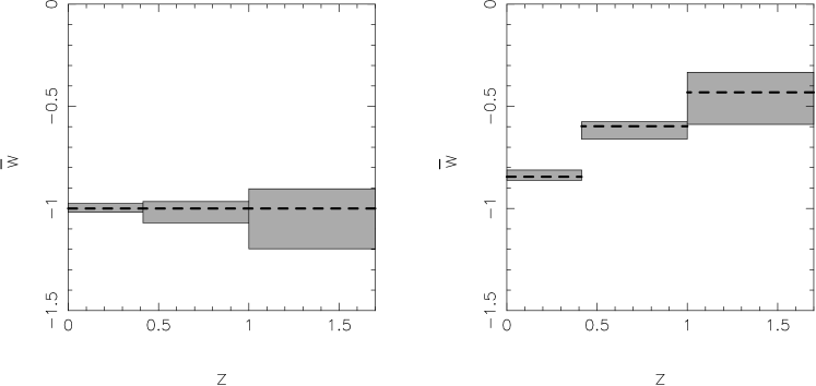
Figure 7: The $w$-probe is reconstructed for the unevolving $\Lambda$CDM model with $w=-1$ (left panel) and an evolving DE model with $w=-1/(1+z)$ (right panel). $1000$ realizations of SNAP-like data have been used. The thick dashed line in both panels indicates the exact value of $\bar{w}$ for the fiducial model, the dark grey boxes in each panel indicate the $1\sigma$ confidence levels on $\bar{w}$ reconstructed for the two models using the double smoothing scheme with $\Delta=0.24$ and marginalising over $\Omega_{0\rm m}=0.3\pm 0.07$. This figure illustrates that the $w$-probe works remarkably well for both $\Lambda$CDM (left panel) and for evolving DE (right panel). The details for this figure are given in Table 3.

We now demonstrate this by showing the results obtained using our smoothing scheme after marginalising over the matter density. We simulate SNAP like data for two models: (a) $\Lambda$CDM and (b) a $w=-1/(1+z)$ ‘metamorphosis’ model. When applying the smoothing scheme, we assume that $\Omega_{0\rm m}$ follows a Gaussian probability distribution with mean $\overline{\Omega_{0\rm m}}=0.3$ and variance $\sigma=0.07$ (the error being commensurate to that expected from the current CMB and Large Scale Structure data (Percival et al., 2001)). In figure 7 and table 3, we show the results for the $w$-probe calculated for the two models. We find that the $w$-probe ($\bar{w}$) is determined to a high degree of accuracy for both the models even when we marginalize over $\Omega_{0\rm m}$ ! The value of $\bar{w}$ for the $\Lambda$CDM model is approximately equal to $-1$, while that for the metamorphosis model shows clear signature of evolution. Thus, even if the matter density of the universe is known uncertainly, this uncertainty does not affect the accuracy of the reconstructed $w$-probe significantly. This is a powerful result since it indicates that unlike the equation of state, the $w$-probe is not overtly sensitive to the value of $\Omega_{0\rm m}$ for SNAP-quality data.

Table 3: The reconstructed $w$-probe $\bar{w}$ (Eq. (5)) over specified redshift ranges (and its $1\sigma$ error) is shown for 1000 realizations of SNAP data. Two fiducial models are used : the $w=-1/(1+z)$ ‘metamorphosis’ model and $w=-1$ ($\Lambda$CDM). We deploy the method of double smoothing with $\Delta=0.24$ and marginalize over $\Omega_{0\rm m}=0.3\pm 0.07$.

	$w=-1/(1+z)$		$w=-1$
$\Delta z$	$\bar{w}$	$\bar{w}_{\rm exact}$	$\bar{w}$	$\bar{w}_{\rm exact}$
$0-0.414$	$-0.837\pm 0.025$	$-0.845$	$-1.003\pm 0.021$	$-1.0$
$0.414-1$	$-0.618\pm 0.042$	$-0.598$	$-1.018\pm 0.052$	$-1.0$
$1-1.7$	$-0.461\pm 0.127$	$-0.432$	$-1.051\pm 0.147$	$-1.0$

From the above results, we see that the $w$-probe is very effective as a diagnostic of dark energy, especially in differentiating between $\Lambda$CDM and other models of dark energy. We summarise some important properties of the $w$-probe below:

1. $\bar{w}(z_{1},z_{2})$ is determined from the first derivative of the luminosity distance. Its reconstructed value is therefore less noisy than the equation of state $w(z)$ (which is determined after differentiating $d_{L}(z)$ twice; compare (4) and (5) ).

2. $\bar{w}(z_{1},z_{2})=-1$ uniquely for concordance cosmology ($\Lambda$CDM). For all other dark energy models $\bar{w}\neq-1$. This remains true when $\bar{w}$ is marginalized over $\Omega_{0\rm m}$.

3. $\bar{w}$ is robust to small uncertainties in the value of the matter density. As we saw earlier this uncertainty can induce large errors in determinations of the cosmic equation of state $w(z)$, see also Maor et al. (2002). The weak dependence of $\bar{w}$ on the value of $\Omega_{0\rm m}$ in the range currently favored by observations $0.2\leq\Omega_{0m}\leq 0.4$ implies that the $w$-probe can cope very effectively with the existing uncertainty in the value of the matter density for SNAP-quality data. Furthermore, since $\bar{w}$ is constructed directly from $\rho_{\rm DE}$, any method which determines either the dark energy density or the Hubble parameter from observations can be used to also determine $\bar{w}$. Note that several excellent methods for determining $\rho_{\rm DE}$ and $H(z)$ have been suggested in the literature (Daly & Djorgovsky, 2003, 2004; Alam et al., 2004; Alam, Sahni & Starobinsky, 2004 a; Wang & Mukherjee, 2004; Wang & Tegmark, 2005), and any of these could be used to great advantage in determining the $w$-probe.

Thus we expect that the $w$-probe may be used as a handy diagnostic for dark energy, especially in discriminating between $\Lambda$CDM and other models of dark energy, for SNAP like datasets. Its efficacy lies in the fact that it is not very sensitive to both the value of the present matter density and also the reconstruction method used.

6 Cosmological Reconstruction applied to other physical models of Dark Energy

In this section we draw the readers attention to the dangers encountered during cosmological reconstruction of atypical dark energy models. There are currently two plausible ways of making the expansion of the universe accelerate at late times. The first approach depends on changing the matter sector of the Einstein equations. Examples of this approach are the quintessence fields. A completely different approach has shown that it is possible to obtain an accelerating universe through modifying the gravity sector (see, for instance, Deffayet, Dvali & Gabadadze (2002); Freese & Lewis (2002); Sahni & Shtanov (2003); Carroll, Hoffman & Trodden (2003); Capozziello, Carloni & Troisi (2003); Nojiri & Odintsov (2003); Dolgov & Kawasaki (2003); Sahni (2005) and references therein). In these models, dark energy should not be treated as a fluid or a field. Instead, it may be better dubbed as ’geometric dark energy’. Indeed the DGP model can cause the universe to accelerate even in the absence of a physical dark energy component. As pointed out in Alam et al. (2003); Sahni (2005), the equation of state is not a fundamental quantity for geometric dark energy. E.g., using $w(z)$ in the reconstruction of such models may result in very strange results, including, for instance, singularities in the equation of state.

$\Delta=0.24$, Double Smoothing

Fiducial Model: Braneworld : $\Omega_{0\rm m}=0.3,\Omega_{l}=1,\Omega_{\Lambda_{b}}=0$

Figure 8: The reconstructed Hubble parameter $H(z)$ for the braneworld model (6) for $1000$ realizations of the SNAP dataset. We use the double smoothing scheme of equations (2) and (4) with $\Delta=0.24$. The dashed line represents the fiducial $\Omega_{0\rm m}=0.3,\Omega_{l}=1,\Omega_{\Lambda_{b}}=0$ braneworld model while the solid lines represent the mean and $1\sigma$ limits around it. We note that the Hubble parameter is very well reconstructed for the braneworld model.

As an example, we consider the braneworld dark energy model proposed in Sahni & Shtanov (2003) described by the following set of equations for a flat universe :

$${H^{2}(z)\over H_{0}^{2}} = \Omega_{0\rm m}(1\!+\!z)^{3}+\Omega_{\sigma}+$$

$$2\Omega_{l}-2\sqrt{\Omega_{l}}\,\sqrt{\Omega_{0\rm m}(1\!+\!z)^{3}+\Omega_{\sigma}+\Omega_{l}+\Omega_{\Lambda_{\rm b}}}$$

$$\Omega_{\sigma} = 1-\Omega_{0\rm m}+2\sqrt{\Omega_{l}(1+\Omega_{\Lambda_{b}})}\,\,,$$ (14)

where the densities $\Omega$ are defined as :

$$\Omega_{0\rm m}={\rho_{0m}\over 3m^{2}H_{0}^{2}},\Omega_{\sigma}={\sigma\over 3m^{2}H_{0}^{2}},\Omega_{l}={1\over l_{c}^{2}H_{0}^{2}},\Omega_{\Lambda_{\rm b}}=-{\Lambda_{\rm b}\over 6H_{0}^{2}}\,\,,$$ (15)

$l_{c}=m^{2}/M^{3}$ being a new length scale ($m$ and $M$ refer respectively to the four and five dimensional Planck masses), $\Lambda_{\rm b}$ the bulk cosmological constant and $\sigma$ the brane tension. In this section we have used $\hbar=c=1$. On short length scales $r\ll l_{c}$ and at early times, one recovers general relativity, whereas on large length scales $r\gg l_{c}$ and at late times brane-related effects become important and may lead to the acceleration of the universe. The ‘effective’ equation of state for this braneworld model is given by

$$\rho=\frac{3H^{2}}{8\pi G}(1-\Omega_{\rm m}(z)),\ p=\frac{H^{2}}{4\pi G}(q(z)-1/2)$$ (16)

$$w_{\rm eff}=\frac{p}{\rho}=\frac{q(z)-1/2}{3(1-\Omega_{\rm m}(z))}\,\,.$$ (17)

It is obvious that the effective equation of state in this braneworld model may become singular if $\Omega_{\rm m}(z)\equiv\Omega_{0\rm m}(1+z)^{3}H_{0}^{2}/H^{2}(z)$ becomes unity. This does not signal any inherent pathologies in the model however. We should remember that the acceleration of the universe in this model is due to modification of the expansion of the universe at late times due to extra-dimensional effects. Hence it is not very appropriate to describe dark energy by an equation of state for such a model. However, it would be interesting to see if the singularity in the effective $w$ for this model can be recovered by our smoothing method.

Fiducial Model: Braneworld : $\Omega_{0\rm m}=0.3,\Omega_{l}=1,\Omega_{\Lambda_{b}}=0$

Figure 9: Reconstructed equation of state for the braneworld model (6) for $1000$ realizations of the SNAP dataset. The left panel shows results for the double smoothing scheme of equations (2) and (4) with $\Delta=0.24$ while the right panel uses the ansatz (18) to reconstruct the equation of state. The dashed line in each panel represents the fiducial $\Omega_{0\rm m}=0.3,\Omega_{l}=1,\Omega_{\Lambda_{b}}=0$ braneworld model while the solid lines represent the mean and $1\sigma$ limits around it.

We attempt to reconstruct an $\Omega_{0\rm m}=0.3,\Omega_{l}=1,\Omega_{\Lambda_{b}}=0$ braneworld model which is a good fit to the current supernova data Alam & Sahni (2002). We simulate data according to SNAP and obtain results for the double smoothing method with $\Delta=0.24$. In figure 8, we show the reconstructed Hubble parameter for this reconstruction. We see that the Hubble parameter is very well reconstructed and shows no pathological behavior.

We now obtain the equation of state of dark energy for this model. For this purpose, we also use an ansatz for the equation of state as suggested by Chevallier & Polarski (2001) and Linder (2003) (the CPL fit)

$$w(z)=w_{0}+\frac{w_{1}z}{1+z}\,\,.$$ (18)

The results are shown in figure 9. We find, as expected, that it is impossible to catch the singularity in the equation of state at $z\simeq 0.8$ using an equation of state ansatz. Of course, one may try and improve upon this somewhat dismal picture by introducing fits with more free parameters. However, it is well known that the presence of more degrees of freedom in the fit leads to a larger degeneracy (between parameters) and hence to larger errors of reconstruction (Weller & Albrecht, 2002). In contrast to this approach, when we reconstruct the equation of state using the smoothing scheme (which does not presuppose any particular behavior of the equation of state), the Hubble parameter is reconstructed very accurately and hence the ‘effective’ equation of state for this model is also reconstructed well, as shown in figure 9. From this figure we see a clear evidence of the singularity at $z\simeq 0.8$. Thus to obtain maximum information about the equation of state, especially in cases where the dark energy model is very different from the typical quintessence-like models, it may be better to reconstruct the Hubble parameter or the dark energy density first.

Therefore, we find that the smoothing scheme, which performs reasonably when reconstructing quintessence models of dark energy models, can be also applied to models which show a departure from general relativistic behavior at late times. This section illustrates the fact that, in general, reconstructing $H(z)$ and its derivatives such as the deceleration parameter $q(z)$ may be less fraught with difficulty than a reconstruction of $w(z)$, which, being an effective equation of state and not a fundamental physical quantity in some DE models, can often show peculiar properties.

7 Conclusion

This paper presents a new approach to analyzing supernova data and uses it to extract information about cosmological functions, such as the expansion rate of the universe $H(z)$ and the equation of state of dark energy $w(z)$. In this approach, we deal with the data directly and do not rely on a parametric functional form for fitting any of the quantities $d_{L}(z),H(z)$ or $w(z)$. Therefore, we expect the results obtained using this approach to be model independent. A Gaussian kernel is used to smooth the data and to calculate cosmological functions including $H(z)$ and $w(z)$. The smoothing scale used for the kernel is related to the number of supernovae, errors of observations and derived errors of the parameters by a simple formula, eq (6). For a given supernova distribution, the smoothing scale determines both the errors on the parameters and the bias of the results (see appendix A). $\Delta$ cannot be increased arbitrarily as this would diminish the reliability of the results. We use a value of $\Delta$ which gives results which have reasonably small bias as well as acceptable errors of $H(z)$ for the SNAP quality data used in our analysis (see section 3). As can be seen from eq (6), when the data improves (i.e., the number of data points increases and/or measurement errors decrease), we expect that the same value of $\Delta$ would result in smaller errors on $H(z)$.

We demonstrate that this method is likely to work very well with future SNAP-like SNe data, especially in reconstructing the Hubble parameter, which encodes the expansion history of the universe. Moreover, our successful reconstruction of the Hubble parameter can also be used to distinguish between cosmological models such as $\Lambda$CDM and evolving dark energy. The method can be further refined, if one wishes to reconstruct the cosmic equation of state to greater accuracy, by double smoothing the data– smoothing the Hubble parameter, after it has been derived from the smoothed luminosity distance, so as to reduce noise in $w(z)$ (as in section 4). The results obtained using the smoothing scheme compare favorably to results obtained by other methods of reconstruction. Another quantity which may be reconstructed to great accuracy is the look-back time of the universe.

An important result of this paper is the discovery that the $w$-probe (originally proposed in Alam et al. (2004)) provides us with an excellent diagnostic of dark energy. We summarize some of the attractive features of this diagnostic below.

(a) The $w$-probe defined in Eqs. (10) and (5) is obtained from the luminosity distance by means of a single differentiation. Therefore, it avoids the pitfalls of $w(z)$ which is obtained from the luminosity distance through a double differentiation – see Eq.(4), and hence is usually accompanied by large errors (see also Maor, Brustein & Steinhardt (2001)).

(b) The $w$-probe is robust to small uncertainties in the value of $\Omega_{0m}$. This attractive property allows us to get around observational uncertainties in the value of $\Omega_{0m}$ currently known to an accuracy of about $30\%$. Indeed, when marginalized over $\Omega_{0m}$, the $w$-probe can be used to great advantage to distinguish between $\Lambda$CDM and other dark energy models for SNAP-quality data.

We therefore conclude that the proposed reconstruction method by smoothing the supernova data appears to be sufficiently accurate and, when applied to SNAP-type observations, should be able to distinguish between evolving dark energy models and a cosmological constant.

The method proposed by us can also be used for other forms of data which deliver the luminosity (or angular size) distance.

8 Acknowledgment

We would like to thank G. Aldering for providing us with the distribution of SNAP supernovae (table 1). UA thanks the CSIR for providing support for this work. AAS was partially supported by the Russian Foundation for Basic Research, grant 05-02-17450, and by the Research Program ‘Astronomy’ of the Russian Academy of Sciences.

Appendix A Smoothing errors and bias

In this section we explore the errors on the cosmological parameters due to the smoothing scheme, as also the bias which enters the results.

A.1 Smoothing errors

The smoothing scheme used in this paper is of the form :

$$y(z)^{s}=y_{G}(z)+\sum_{i=1}^{N}[y(z_{i})-y_{G}(z_{i})]S(z_{i};\Delta)/\sum_{i=1}^{N}S(z_{i};\Delta)\,\,,$$ (19)

where the quantity $S(z_{i};\Delta)$ represents the smoothing function with a scale $\Delta$ and $y_{G}(z)$ is the subtracted guess model. The quantity being smoothed (in this case $\ln d_{L}$) is represented by $y$, while $y^{s}$ represents the smoothed result. Let the errors in the data at any redshift $z_{i}$ be given by $\sigma_{y}(z_{i})$ and the errors in the guess model be $\sigma_{y_{G}}(z_{i})$. If we look at the second term on the right hand side of eq (19), we see that the errors on this term would be approximately given by the errors on $y$ weighted down by the smoothing scale $\Delta$ and the number of data points $N$. Therefore the error on the smoothed result is:

$$\sigma_{y_{s}}^{2}(z)\simeq\sigma_{y_{G}}^{2}(z)+\frac{\sigma_{y}^{2}(z)+\sigma_{y_{G}}^{2}(z)}{N\Delta}\,\,.$$ (20)

We now consider the errors for an iterative method. The first guess is an exact model, $\Lambda$CDM. Therefore the error on the result of the first iteration is simply

$$\sigma_{y_{1}}^{2}(z)\simeq\frac{\sigma_{y}^{2}(z)}{N\Delta}\,\,.$$ (21)

The next guess model is $y_{1}(z)$. Therefore the error on the result is

$$\sigma_{y_{2}}^{2}(z)\simeq\left(2+\frac{1}{N\Delta}\right)\frac{\sigma_{y}^{2}(z)}{N\Delta}\,\,.$$ (22)

From this we can show that the errors on the result for the M-th iteration is :

$$\sigma_{y_{M}}^{2}(z) \simeq \left[1+\sum_{i=1}^{M-1}\left(1+\frac{1}{N\Delta}\right)^{i}\right]\frac{\sigma_{y}^{2}(z)}{N\Delta}$$ (23)

$$\simeq \left[M+\frac{M(M-1)}{2N\Delta}\right]\frac{\sigma_{y}^{2}(z)}{N\Delta}\,\,.$$

The second term on the right-hand side is small for a reasonable number of iterations, since $N\simeq 2000$ and $\Delta>0.01$ usually. Therefore we may approximate the errors on the log luminosity distance after $M$ iterations for the guess model as

$$\sigma_{\ln d_{L}}^{M}(z)=\sqrt{M}\sigma_{\ln d_{L}}^{0}(z)\,\,,$$ (24)

where $\sigma_{\ln d_{L}}^{0}(z)$ is the error for a simple smoothing scheme where the data is smoothed without using a guess model.

Figure 10: Comparison of the reconstructed parameters obtained by using the smoothing method (25) with the variable $\Delta(z)=0.2z/(1+z)^{2}$ for the $\Lambda CDM$ model (the dotted line in each panel) with the analytical biased result given by Eq. (30) (dashed line). The solid line represents the fiducial $\Lambda CDM$ model. Note the excellent agreement between the analytical and numerical results in the redshift range $0.1\lower 3.48746pt\hbox{ $\buildrel<\over{\sim}$}~{}z\lower 3.48746pt\hbox{ $\buildrel<\over{\sim}$}~{}1.1$.

A.2 Smoothing Bias

In any kind of a smoothing scheme for the luminosity distance, some bias is introduced both in it and in derived quantities like $H(z)$ and $w(z)$. To illustrate the effect of this bias, we calculate it for the simplest Gaussian smoothing scheme for $\ln d_{L}(z)$ with the width $\Delta(z)\ll 1$ :

$$\ln d_{L}(z)^{\rm s}=N(z)\sum_{i=1}^{M}\ln d_{L}(z_{i}){\rm exp}\left[-\frac{(z-z_{i})^{2}}{2\Delta^{2}}\right]~{},$$ (25)

$$N(z)^{-1}=\sum_{i=1}^{M}{\rm exp}\left[-\frac{(z-z_{i})^{2}}{2\Delta^{2}}\right],\hskip 62.59596pt$$ (26)

where M is the total number of supernovae data points. The bias at each redshift (${\cal B}(z)=\ln d_{L}(z)^{\rm s}-\ln d_{L}(z)$) is the difference between the smoothed $\ln d_{L}(z)$ and the exact value of $\ln d_{L}(z)$ :

$${\cal B}(z)=N(z)\sum_{i=1}^{M}(\ln d_{L}(z_{i})-\ln d_{L}(z))\ {\rm exp}\left[-\frac{(z-z_{i})^{2}}{2\Delta^{2}}\right]\,\,.$$ (27)

Expanding $\ln d_{L}(z_{i})$ in terms of $\ln d_{L}(z)$ and its derivatives by Taylor expansion, we get:

$${\cal B}(z)=N(z)\sum_{i=1}^{M}\left[(\ln d_{L}(z))^{\prime}(z_{i}-z)+(\ln d_{L}(z))^{\prime\prime}\frac{(z_{i}-z)^{2}}{2}\right]$$

$${\large\times}\ {\rm exp}\left[-\frac{(z-z_{i})^{2}}{2\Delta^{2}}\right],$$ (28)

where the prime denotes the derivative with respect to $z$ and we neglect higher derivatives. To see the effect of this bias at low and high redshifts where the number of supernovae on both sides of each $z$ are not equal, we rewrite Eq. (28) in another way. Let $\delta$ be the spacing between two neighboring data points, so that $z=m\delta$. For $m<M/2$, we have:

$${\cal B}(z)=\hskip 221.93158pt$$

$$N(z)\sum_{i=1}^{2m}\left[(\ln d_{L}(z))^{\prime\prime}\frac{\delta^{2}(i-m)^{2}}{2}\right]{\rm exp}\left[-\frac{\delta^{2}(i-m)^{2}}{2\Delta^{2}}\right]$$

$$+N(z)\sum_{i=2m+1}^{M}\left[(\ln d_{L}(z))^{\prime}\delta(i-m)+(\ln d_{L}(z))^{\prime\prime}\frac{\delta^{2}(i-m)^{2}}{2}\right]$$

$${\large\times}\ {\rm exp}\left[-\frac{\delta^{2}(i-m)^{2}}{2\Delta^{2}}\right] \,\,,$$

and for $m>M/2$:

$${\cal B}(z)=\hskip 221.93158pt$$

$$N(z)\sum_{i=2m-M+1}^{M}\left[(\ln d_{L}(z))^{\prime\prime}\frac{\delta^{2}(i-m)^{2}}{2}\right]{\rm exp}\left[-\frac{\delta^{2}(i-m)^{2}}{2\Delta^{2}}\right]$$

$$+N(z)\sum_{i=1}^{2m-M}\left[(\ln d_{L}(z))^{\prime}\delta(i-m)+(\ln d_{L}(z))^{\prime\prime}\frac{\delta^{2}(i-m)^{2}}{2}\right]$$

$${\large\times}\ {\rm exp}\left[-\frac{\delta^{2}(i-m)^{2}}{2\Delta^{2}}\right]$$

The first term in the above equations is the general bias of the method, while the second term is the bias arising due to an asymmetric number of data points around each supernova. For $m=M/2$, the number of data points is the same from both sides and we have:

$${\cal B}(z)=N(z)\sum_{i=1}^{M}\left[(\ln d_{L}(z))^{\prime\prime}\frac{\delta^{2}(i-m)^{2}}{2}\right]{\rm exp}\left[-\frac{\delta^{2}(i-m)^{2}}{2\Delta^{2}}\right].$$

In the continuous limit where $x=i-m$ is assumed, we get:

$${\cal B}(z) = N(z)\int[(\ln d_{L}(z))^{\prime\prime}\frac{\delta^{2}x^{2}}{2}]{\rm exp}\left[-\frac{\delta^{2}x^{2}}{2\Delta^{2}}\right]dx~{},$$ (29)

$$N(z) = \int{\rm exp}\left[-\frac{\delta^{2}x^{2}}{2\Delta^{2}}\right]dx\,\,.$$

Therefore, the bias has the simple form

$${\cal B}(z)=\frac{(\ln d_{L}(z))^{\prime\prime}\delta^{2}}{2\delta^{2}/\Delta^{2}}=\frac{\Delta^{2}}{2}(\ln d_{L}(z))^{\prime\prime}\,\,.$$ (30)

This is a good analytical approximation for the bias at redshifts in the middle range, where we do not encounter the problem of data asymmetry. To see the effect of this bias, let us assume that the real model is the standard $\Lambda CDM$, add the bias term to this model and then calculate the biased $H(z)$ and $w(z)$. The result from this analytical calculation can be compared to the result of smoothing the exact $\Lambda CDM$ model using our method. The figure 10 simply illustrates that the results obtained using Gaussian smoothing and by the use of formula (30) are in good agreement in the middle range of redshifts. However, we do not expect the formula (30) to work properly at very low ($z<0.1$) and high ($z>1$) redshifts where the above mentioned asymmetry of points adds a further bias.

Also, it appears that the smoothing bias has a tendency to decrease $w(z)$ below its actual value in the middle range of $z$. Thus, $\Lambda CDM$ may appear to be a ‘phantom’ ($w<-1$) if too large a smoothing scale is chosen.

Appendix B Exploring smoothing with variable width $\Delta(z)$

$\Delta=1.2\,{\frac{z}{(1+z)^{2}}}$

Fiducial Model: $w=-0.5$

Figure 11: The smoothing scheme of equation (2) is used with $\Delta(z)=1.2\,z/(1+z)^{2}$ to obtain smoothed $H(z)$ and $w(z)$ from $1000$ realizations of the SNAP dataset. The panel (a) represents the form of $\Delta(z)$ used, while panels (b) and (c) represent the reconstructed $H(z)$ and $w(z)$. The dashed line in panels (b) and (c) represents the fiducial ‘metamorphosis’ model with $w=-0.5$ while the solid lines represent the mean and $1\sigma$ limits around it. The dotted line is $\Lambda$CDM.

$\Delta=0.36\,{\rm tanh}\,{\frac{0.23+z}{0.64}}$

Fiducial Model: $w=-0.5$

Figure 12: The smoothing scheme of equation (2) is used with a tangent hyperbolic form of variable $\Delta(z)$ to obtain smoothed $H(z)$ and $w(z)$ from $1000$ realizations of the SNAP dataset. The panel (a) represents the form of $\Delta(z)$ used, while panels (b) and (c) represent the reconstructed $H(z)$ and $w(z)$. The dashed line in panels (b) and (c) represents the fiducial $w=-0.5$ ‘metamorphosis’ model while the solid lines represent the mean and $1\sigma$ limits around it. The dotted line is $\Lambda$CDM.

In order to deal with the problem of data asymmetry and paucity at low and high redshifts we may consider using a variable $\Delta(z)$. (i) Low $z$ ($z_{*}\ll 1$) : in this case, there are many more supernovae at $z>z_{*}$ than there are at $z<z_{*}$. The error-bars are also small in the low redshift region. Therefore, a smaller value of $\Delta$ appears to be more appropriate at low $z$. (ii) High $z$ ($z_{*}>1$) : in this case, there is considerably more data at $z<z_{*}$ than at $z>z_{*}$. However, at high $z$ the errors are considerably larger than at low $z$, which suggests that in order to avoid a noisy result we must use a larger value of $\Delta$ in this region. In this section, we investigate two different functional forms of $\Delta(z)$ with the above properties and show how they result in the reconstruction of the equation of state.

B.1 $\Delta(z)=\Delta_{0}z/(1+z)^{2}$

In section 2 we mentioned that, for $|z-z_{i}|\ll 1$, the exponent in Eq. (2) reduces to the form $-(z-z_{i})^{2}/2\Delta^{2}(1+z)^{2}$ and the effective Gaussian smoothing scale becomes $\Delta(1+z)$. So if we use a variable $\Delta(z)=\Delta_{0}z/(1+z)^{2}$ then the effective Gaussian smoothing scale approaches a constant at large $z$ and tends to a small value at small $z$. The results obtained using this method are shown in figure 11 for SNAP data, using the model $w=-0.5$. We find that, the result for the Hubble parameter does not change much. However, the equation of state is somewhat better reconstructed, but noisier at low redshift because of the small width of smoothing.

B.2 tan-hyperbolic form of $\Delta(z)$

Tangent hyperbolic form for $\Delta(z)$ is another form of the variable $\Delta(z)$ which can simultaneously satisfy both the low and high $z$ requirements. It has a small value at low redshifts and a bigger value at the higher redshifts. An additional important property of this function is that it changes smoothly from low to high $z$, which translates into a smoother second derivative $w(z)$ – see (2) - (4).

A drawback of this method is that the tangent hyperbolic function introduces a number of free parameters into the problem. However the role of these parameters can be understood as follows. The tangent hyperbolic function can be written in the general form

$$\Delta(z)\,=\,a\,{\rm tanh}\,{\frac{b+z}{c}}~{}.$$ (31)

As we saw earlier, if $\Delta$ is held constant, then optimal results are obtained for $\Delta_{0}\,=\,0.24$ in (2) when we use bootstrap iterative process. We therefore determine $a,b$ and $c$ in (31) so that $\Delta(z)\approx\frac{1}{2}\Delta_{0}$ at $z\approx 0$, and $\Delta(z)\approx\frac{3}{2}\Delta_{0}$ at $z\approx 1.7$; consequently

$$\Delta(z)\,=\,0.36\,{\rm tanh}\,{\frac{0.23+z}{0.64}}~{}.$$ (32)

The results obtained using this method are shown in figure 12 for SNAP data for the fiducial model $w=-0.5$. We find that this variable form of $\Delta(z)$ leads to a slight improvement of results at low redshifts by getting rid of the small bias which remains in the bootstrap iterative process. This improvement of the results is expected especially for the cosmological models whose equation of state at low redshift is very different as compared to the $\Lambda$CDM model, which is our initial guess model.

References

- Alam & Sahni (2002) U. Alam and V. Sahni, 2002, astro-ph/0209443.
- Alam et al. (2003) U. Alam, V. Sahni, T. D. Saini and A. A. Starobinsky, 2003, Mon. Not. Roy. Ast. Soc. 344, 1057.
- Alam et al. (2004) U. Alam, V. Sahni, T. D. Saini and A. A. Starobinsky, 2004, Mon. Not. Roy. Ast. Soc. 354, 275.
- Alam, Sahni & Starobinsky (2004 a) U. Alam, V. Sahni and A. A. Starobinsky, 2004 a, JCAP 0406 008.
- Alam et al. (2004 b) U. Alam, V. Sahni, T. D. Saini and A. A. Starobinsky, 2004 b, astro-ph/0406672.
- Aldering et al. (2004) G. Aldering et al., 2004, astro-ph/0405232
- Basset, Corasaniti & Kunz (2004) B. Bassett, P. S. Corasaniti and M. Kunz, 2004, Astroph. J. 617, L1-L4.
- Capozziello, Carloni & Troisi (2003) S. Capozziello, S. Carloni and A. Troisi, 2003, ”Recent Research Developments in Astronomy & Astrophysics”-RSP/AA/21-2003 [astro-ph/0303041].
- Carroll (2001) S. M. Carroll, 2001, Living Rev.Rel. 4, 1.
- Carroll, Hoffman & Trodden (2003) S. M. Carroll, M. Hoffman and M. Trodden, 2003, Phys. Rev. D 68, 023509.
- Chevallier & Polarski (2001) M. Chevallier and D. Polarski, 2001, IJMP D 10, 213.
- Chiba & Nakamura (2000) T. Chiba and T. Nakamura, 2000, Phys. Rev. D 62, 121301(R).
- Coles & Lucchin (1995) P. Coles and F. Lucchin, 1995, ”Cosmology, The origin and evolution of large scale structure”, John Wiley & sons.
- Corasaniti & Copeland (2003) P. S. Corasaniti and E. J. Copeland, 2003, Phys. Rev. D 67, 063521.
- Daly & Djorgovsky (2003) R. A. Daly and S. G. Djorgovsky, 2003, Astroph. J. 597, 9.
- Daly & Djorgovsky (2004) R. A. Daly and S. G. Djorgovsky, 2004, Astroph. J. 612, 652.
- Deffayet, Dvali & Gabadadze (2002) C. Deffayet, G. Dvali and G. Gabadadze, 2002, Phys. Rev. D 65, 044023.
- Dolgov & Kawasaki (2003) A. D. Dolgov and M. Kawasaki, 2003, Phys.Lett. B 573, 1.
- Espana-Bonet & Ruiz-Lapuente (2005) C. Espana-Bonet, P. Ruiz-Lapuente, 2005, hep-ph/0503210.
- Freese & Lewis (2002) K. Freese and M. Lewis, 2002, Phys. Lett. B 540, 1.
- Gerke & Efstathiou (2002) B. Gerke and G. Efstathiou, 2002, Mon. Not. Roy. Ast. Soc. 335, 33.
- Gong (2005 a) Y. Gong, 2005 a, IJMP D 14, 599.
- Gong (2005 b) Y. Gong, 2005 b, CQG 22 2121.
- Guo, Ohta & Zhang (2005) Z-K. Guo, N. Ohta, Y-Z. Zhang, 2005, Phys. Rev. D 72, 023504.
- Huterer & Starkman (2003) D. Huterer and G. Starkman, 2003, Phys. Rev. Lett. 90, 031301.
- Huterer & Turner (1999) D. Huterer and M. S. Turner, 1999, Phys. Rev. D 60, 081301.
- Kamenshchik, Moschella & Pasquier (2001) A. Kamenshchik, U. Moschella and V. Pasquier, 2001, Phys. Lett. B 511, 265.
- Knop et al. (2003) R. A. Knop et al., 2003, Astroph. J. 598, 102(K).
- Lazkoz, Nesseris & Perivelaroupolos (2005) R. Lazkoz, S. Nesseris and L. Perivolaroupolos, 2005, astro-ph/0503230.
- Linder (2003) E. V. Linder, 2003, Phys. Rev. Lett. 90, 091301.
- Linder (2004) E. V. Linder, 2004, hep-th/0410017.
- Maor et al. (2002) I. Maor, R. Brustein, J. McMahon and P. J. Steinhardt, 2002, Phys. Rev. D 65, 123003.
- Maor, Brustein & Steinhardt (2001) I. Maor, R. Brustein and P. J. Steinhardt, 2001, Phys. Rev. Lett. 86, 6.
- Martinez & Saar (2002) V. J. Martinez and E. Saar, 2002, ”Statistics of Galaxy Distribution”, Chapman & Hall.
- Nakamura & Chiba (1999) T. Nakamura and T. Chiba, 1999, Mon. Not. Roy. Ast. Soc. 306, 696.
- Nesseris & Perivelaroupolos (2004) S. Nesseris and L. Perivolaroupolos, 2004, Phys. Rev. D 70 043531.
- Nojiri & Odintsov (2003) S. Nojiri and S.D. Odintsov, 2003, Phys.Rev. D 68, 123512.
- Padmanabhan (2003) T. Padmanabhan, 2003, Phys. Rep. 380, 235.
- Peebles & Ratra (2003) P. J. E. Peebles and B. Ratra, 2003, Rev.Mod.Phys. 75, 559.
- Percival et al. (2001) W. J. Percival et al., 2001, Mon. Not. Roy. Ast. Soc. 327, 1297.
- Perlmutter et al. (1999) S. J. Perlmutter et al., 1999, Astroph. J. 517, 565.
- Ratra & Peebles (1988) B. Ratra and P. J. E. Peebles, 1988, Phys. Rev. D 37, 3406.
- Riess et al. (1998) A. G. Riess et al., 1998, Astron. J. 116, 1009.
- Riess et al. (2004) A. G. Riess et al., 2004, Astroph. J. 607, 665(R).
- Sahni (2004) V. Sahni, 2004, Dark Matter and Dark Energy, Lectures given at the 2nd Aegean Summer School on the Early Universe, Ermoupoli, Island of Syros, Greece, astro-ph/0403324.
- Sahni (2005) V. Sahni, 2005, Cosmological Surprises from Braneworld models of Dark Energy, Proceedings of the 14th Workshop on General relativity and Gravitation (JGRG14), Kyoto University, Japan, 29 November - 3 December, 2004. Ed. by W. Hikida, M. Sasaki, T. Tanaka and T. Nakamura; pp. 95 - 115 [astro-ph/0502032].
- Sahni & Coles (1995) V. Sahni and P. Coles, 1995, Phys.Rept. 262, 1-135.
- Sahni et al. (2003) V. Sahni, T. D. Saini, A. A. Starobinsky and U. Alam, 2003, JETP Lett. , 77, 201.
- Sahni & Shtanov (2003) V. Sahni and Yu. V. Shtanov, 2003, JCAP 0311, 014.
- Sahni & Shtanov (2005) V. Sahni and Yu. Shtanov, 2005, Phys. Rev. D 71, 084018.
- Sahni & Starobinsky (2000) V. Sahni and A. A. Starobinsky, 2000, IJMP D 9, 373.
- Sahni & Wang (2000) V. Sahni and L. Wang, 2000, Phys. Rev. D 62 103517.
- Saini (2003) T. D. Saini, 2003, Mon. Not. Roy. Ast. Soc. 344, 129.
- Saini et al. (2000) T. D. Saini, S. Raychaudhury, V. Sahni and A. A. Starobinsky, 2000, Phys. Rev. Lett. 85, 1162.
- Saini, Weller & Bridle (2004) T. D. Saini, J. Weller and S. L. Bridle, 2004, Mon. Not. Roy. Ast. Soc. 348, 603.
- Simon, Verde & Jimenez (2005) J. Simon, L. Verde and R. Jimenez, 2005, Phys. Rev. D 71, 123001.
- Starobinsky (1998) A. A. Starobinsky, 1998, JETP Lett. 68, 757.
- Tegmark (2002) M. Tegmark, 2002, Phys. Rev. D , 66 103507.
- Tonry et al. (2003) J. L. Tonry et al., 2003, Astroph. J. 594, 1.
- Wang & Lovelace (2001) Y. Wang and G. Lovelace, 2001, Astroph. J. 562, L115.
- Wang & Mukherjee (2004) Y. Wang and P. Mukherjee, 2004, Astroph. J. 606, 654.
- Wang & Tegmark (2005) Y. Wang and M. Tegmark, 2005, Phys. Rev. D 71, 103513.
- Weller & Albrecht (2002) J. Weller and A. Albrecht, 2002, Phys. Rev. D 65, 103512.