How many dark energy parameters?

Abstract

For exploring the physics behind the accelerating universe a crucial question is how much we can learn about the dynamics through next generation cosmological experiments. For example, in defining the dark energy behavior through an effective equation of state, how many parameters can we realistically expect to tightly constrain? Through both general and specific examples (including new parametrizations and principal component analysis) we argue that the answer is 42 – no, wait, two. Cosmological parameter analyses involving a measure of the equation of state value at some epoch (e.g. $w_{0}$) and a measure of the change in equation of state (e.g. $w^{\prime}$) are therefore realistic in projecting dark energy parameter constraints. More elaborate parametrizations could have some uses (e.g. testing for bias or comparison with model features), but do not lead to accurately measured dark energy parameters.

I Introduction

The discovery of the acceleration of the cosmic expansion has thrown physics and astronomy research into a ferment of activity, from a search for fundamental theories to investigation of parametrizations relating models and the cosmological dynamics to development of astrophysical surveys yielding improved measurements. The question of the nature of the accelerating mechanism (“dark energy”) impacts the composition of some 70% of the energy density of the universe, the evolution of large scale structure, and the fate of the universe. Learning the physics responsible will advance the fundamental frontiers of science, in high energy physics, extra dimensions, gravity beyond Einstein relativity, or possibly the unification of gravity and quantum physics.

Given the open landscape of proposed theories, it is difficult to assess the prospects for a definitive measurement of the physics. We consider here how much information the next generation of cosmological measurements is likely to realistically provide on the nature of dark energy. By “realistically”, we mean several things. Knocking down theories one by one is unlikely to be useful, given theorists’ fecundity and fickleness. Direct reconstruction, whether of the dark energy equation of state, density, or potential, while formally possible (in a limited range at least), is stymied by statistical and systematic errors in the observations. So the question becomes, while describing dark energy in as model independent fashion as possible, what is the greatest degree of informative parametrization justified by the future observations.

In §II we examine various parametrizations, including designing some new ones useful for studying aspects of the dark energy dynamics, utilizing one to four parameters. In §III we define success criteria for a parameter estimation and project what constraints future supernova distance, CMB, and weak lensing shear measurements can impose, analyzing the resulting maximum number of parameters tightly fit. Discussion of trade offs between success and model independence, such as in the minimum variance approach, is another issue addressed. We consider in §IV uncorrelated and non-parametric characterizations. §V examines what the data requirements would be to obtain more information on the nature of dark energy and summarizes the conclusions on the viable number of dark energy parameters.

II Modeling Dark Energy

Dark energy appears in the Friedmann equations of cosmological dynamics through its effective energy density and pressure. We emphasize that these need only be effective quantities and not necessarily correspond to characteristics of a physical scalar field, say. The ratio of the energy density to pressure, known as the equation of state ratio $w$, has importance within the equations regardless of its physical origin. This has been emphasized by linjen (see also sahni ), in that any deviation of the Hubble parameter $H=\dot{a}/a$ from the matter dominated behavior can be written in terms of an effective equation of state.

So a function $w(a)$, where $a$ is the scale factor of the universe, is key to understanding the dynamics of the cosmological expansion, in particular its acceleration. With only imperfect knowledge of the expansion history $a(t)$, through noisy distance measures over a finite redshift range, one cannot derive the full function $w(a)$. The minimum characteristics one would seek to provide insight on the origin of the acceleration and nature of the dark energy would be a measure of $w$ at some epoch, e.g. today, and a measure of its dynamics, i.e. its change over time (see caldlin for a demonstration of the strength of this approach; see our §V for a discussion of the role of sound speed). In particular these could yield consistency or conflict with the two key properties of the cosmological constant as the explanation: $w$ unchanging and equal to $-1$.

Within a realistic scenario of next generation observations, how much can we expect to learn about the dark energy function $w(a)$? We consider three approaches to answering this question. After reviewing the basis for the current two parameter model, in §II.1 we attempt to generalize it with a phenomenological approach, calling out a set of four characteristics of an evolving equation of state, and then examining restrictions of the phase space. In §II.2 we instead extend the two parameter model with physically motivated third parameters. Later, for a more dark energy model independent tack, in §IV we investigate a principal component approach.

II.1 Describing Dark Energy Evolution

The two basic characteristics of a dynamical function mentioned above – a value and a change in value – can be implemented in many ways. The one in perhaps most common use presently is employing the present value $w_{0}$ and the logarithmic derivative with respect to scale factor, $w^{\prime}\equiv dw/d\ln a$, at redshift $z=1$ ($a=1/2$):

$$w(a) = w_{0}-2w^{\prime}(1-a)$$ (1)

$$= w_{0}+w_{a}(1-a).\qquad{\rm[Model\ 2.0]}$$

This possesses many useful properties, including a close approximation to a wide variety of dark energy dynamics, boundedness at early times (so CMB observations can be readily treated), analyticity of the Hubble parameter expression (involving an integral over $w$), and ease of physical interpretation linprl ; lingrav .

To go beyond this description of dark energy dynamics, one might characterize the physics in a broadly phenomenological manner as having some equation of state value far in the past, $w_{p}$, (deep in the matter dominated epoch, near the time of CMB last scattering, say), some value far in the future, $w_{f}$, (deep in the dark energy dominated epoch), and treat the transition between the two as occurring at some scale factor $a_{t}$ and with some rapidity $\tau$.

We choose to treat the transition in terms of the e-fold variable $N=\ln a$, since this is the characteristic scale of the cosmological background evolution. That is, any dynamics driven purely by the expansion will have a transition scale length of order one in this variable. If the equation of state changes according to $\dot{w}\sim H$, then $w^{\prime}=dw/dN\sim 1$.

In the neighborhood of the transition we can write

$$w(N)\approx w_{t}\left[1+(N-N_{t})\frac{1}{w_{t}}\frac{dw}{dN_{t}}\right].$$ (2)

There are many possible ways to extend this to a full function describing the past and future evolution of the equation of state. We would like this to be bounded in both directions (i.e. the past $N\ll N_{t}$ and the future $N\gg N_{t}$). We choose to view Eq. (2) as the first order term in an exponential, and applying our boundedness criteria we adopt

$$w(N)=w_{f}+\frac{\Delta w}{1+e^{(N-N_{t})/\tau}},\qquad{\rm[Model\ 4.0]}$$ (3)

where $\Delta w=w_{p}-w_{f}$. Note that $\tau=\Delta w/[4(-dw/dN_{t})]$.

This is similar to the four parameter equation of state proposed by ccl ,

$$w(a)=w_{0}+(w_{m}-w_{0})\frac{1+e^{a_{c}/\Delta}}{1-e^{1/\Delta}}\frac{1-e^{(1-a)/\Delta}}{1+e^{(a_{c}-a)/\Delta}},$$ (4)

due to a similar phenomenology, but Model 4.0 has some advantages. The previous version carried out the transition in $a$ rather than $N$ (also cf. bassett ), and so there was no natural scale for the transition rapidity, unlike the present case. Also, Model 4.0 allows integration over $w$ to be done analytically and so the Hubble parameter can be written explicitly. Note that Eq. (3) is equivalent to

$$w(a)=w_{f}+\frac{\Delta w}{1+(a/a_{t})^{1/\tau}},\qquad{\rm[Model\ 4.0]}$$ (5)

and so

$$H^{2}/H_{0}^{2} = \Omega_{m}a^{-3}+(1-\Omega_{m})(1+a_{t}^{1/\tau})^{-3\tau^{\prime}}\times$$ (6)

$$\ a^{-3(1+w_{f})}[1+(a/a_{t})^{-1/\tau}]^{3\tau^{\prime}},$$

where $\Omega_{m}$ is the dimensionless matter density, $\tau^{\prime}=\tau\Delta w$, and we assume a spatially flat universe (as throughout this article).

Our complete set of cosmological parameters for distance data then becomes $\{{\cal M},\Omega_{m},w_{f},\Delta w,a_{t},\tau\}$, where ${\cal M}$ is a nuisance parameter combining supernova absolute magnitude and the Hubble constant $H_{0}$. The fourth of the dark energy parameters, measuring the rapidity, can be chosen to be $dw/dN_{t}$ rather $\tau$ if desired. This is one new equation of state model we will consider; one unfortunate aspect is that Model 4.0 does not reduce to Model 2.0 for any choice of parameters, so it cannot be viewed as an extension of the “baseline” Model 2.0.

II.2 Extending Two Parameter Dynamics

Given the successful properties of the two parameter model, and that extensive estimation of constraints on the two model parameters exists for present and next generation cosmological probes, let us attempt to extend Model 2.0 to a third parameter, while keeping the virtues as intact as possible. Studies of many dark energy models in the $w^{\prime}-w$ phase plane reveal interesting properties of the dynamics caldlin and show the success – and limitations – of Model 2.0.

This model keeps the derivative $dw/da$ constant, or the logarithmic derivative $w^{\prime}\equiv dw/dN\equiv dw/d\ln a\sim a$. One might conjecture that the logarithmic derivative, giving the change in dark energy equation of state per e-fold of cosmic expansion, is an important characteristic of the dynamics linmiq ; so let us venture a generalization by enlarging its scope of behavior. (A different approach in terms of changing the transition epoch is considered by rapetti .) We consider $w^{\prime}\sim a^{b}$:

$$w(a)=w_{0}+w_{a}(1-a^{b}).\qquad{\rm[Model\ 3.1]}$$ (7)

Since Model 2.0 is a fairly successful approximation for many dark energy models we might expect that $b$ does not deviate greatly from unity. In terms of the phase space dynamics of caldlin , their “thawing” models are a special case of Model 3.1, with $w_{a}=-(1+w_{0})$ and their slope equal to our $b$.

Of course for a model with $w_{a}=0$ (such as taking the cosmological constant as the fiducial model), observations will place no constraints on the third parameter $b$. Therefore, this is not a general extension of the two parameter model. So we also consider a different way of changing the dynamics $w^{\prime}$. We introduce some scale factor dependence to $dw/da$ by adding a term of higher order in $1-a$:

$$w(a)=w_{0}+w_{a}(1-a)+w_{3}(1-a)^{3}.\qquad{\rm[Model\ 3.2]}$$ (8)

Using the cubic power rather than a quadratic preserves the trend of the logarithmic derivative $w^{\prime}$ at the present, $a=1$. For example if $w_{a}=0$ then with this cubic the sign of $w^{\prime}$ does not flip around the present day, unlike with a quadratic. We make no claims, however, that the cubic form is of great significance; it merely represents a possible three parameter form with reasonable properties, extending the standard two parameter model.

It is instructive to also investigate a more extreme evolution of the equation of state, such as

$$w(a)=w_{0}+w_{a}(1-a)+w_{e}[(1+z)e^{z}-1],\quad{\rm[Model\ 3.3]}$$ (9)

to see the influence of runaway behavior at high redshifts. This will not be suitable for treating CMB or growth related data, and we only consider it briefly.

Below we give the expressions for the modifications to the Hubble expansion $\delta H^{2}=H^{2}/H_{0}^{2}-\Omega_{m}a^{-3}$, divided by $(1-\Omega_{m})$, for the models considered:

$${\rm[Model\ 3.1]:} \!\!\!\!\!\!a^{-3(1+w_{0}+w_{a})}e^{-3w_{a}(1-a^{b})/b}$$ (10)

$${\rm[Model\ 3.2]:} \!\!\!\!\!\!a^{-3(1+w_{0}+w_{a}+w_{3})}\times$$

$$\!\!\!\!\!\!e^{-3w_{a}-11w_{3}/2+3(w_{a}+3w_{3})a-9w_{3}a^{2}/2+w_{3}a^{3}}$$

$${\rm[Model\ 3.3]:} \!\!\!\!\!\!a^{-3(1+w_{0}+w_{a}-w_{e})}e^{-3w_{a}(1-a)+3w_{e}(e^{z}-1)}$$ (12)

III Searching for Successful Constraints

One question to address before further investigation is what is our criteria for success in constraining dark energy parameters. We can obviously fit a model with many parameters, each poorly, but what we mean by “how many dark energy parameters?” is how many can we determine to an accuracy that provides real physical insight. What the criteria for success should be is not a solved problem, though recent progress has been made by caldlin ; linbw .

We adopt the following unrigorous but reasonable seeming criteria: 1) a parameter describing the equation of state at some epoch should be determined to a fractional error of $<10\%$, relative to its fiducial value, e.g. the future equation of state value should be found to within 0.1, and 2) a parameter describing the change in equation of state, or a derivative, should be estimated to within 0.2 (i.e. 20% of the Hubble time scale). It is hard to see that much looser constraints would be of substantial use in unraveling the physics.

We carry out a full Fisher analysis of the cosmological parameter uncertainties to test how many equation of state parameters can be reasonably constrained, in addition to the matter density $\Omega_{m}$, and other parameters relevant to the cosmological measurements. Three types of cosmological probes are considered: Type Ia supernova distances (SN), weak lensing shear (WL), and the cosmic microwave background (CMB) angular power spectrum. We employ supernova distance data of the quality expected from the next generation experiment SNAP snap , with 2000 supernovae from $z=0.1-1.7$ plus 300 local supernovae from $z=0.03-0.08$, with intrinsic magnitude dispersion 0.15 magnitudes (7% in luminosity distance) plus an irreducible systematic of $0.02(1+z)/2.7$ mag per 0.1 redshift bin. This method carries with it the parameter ${\cal M}$ to be marginalized over.

For the fiducial weak lensing survey we assume sky coverage of 1000 sq. deg. with 100 galaxies per arcmin², which roughly corresponds to coverage and depth expected from SNAP wliii . We also briefly consider a LSST-type survey with 15000 sq. deg. and 30 galaxies per arcmin². Throughout we consider lensing tomography with 10 redshift bins equally spaced between $z=0$ and $z=3$ and use the lensing power spectra on scales $50\leq\ell\leq 3000$. Intrinsic shape noise of each galaxy is fixed to $\sigma_{\gamma}=0.22$. In addition to the dark energy parameters (those describing the equation of state, plus $\Omega_{m}$) we vary the the amplitude of mass fluctuations with the fiducial value $\sigma_{8}=0.9$, the physical matter and baryon densities $\Omega_{m}h^{2}=0.147$ and $\Omega_{b}h^{2}=0.023$, and the scalar spectral index $n=1.0$. The sum of the neutrino masses is held fixed at $m_{\nu}=0.1$eV. We compute the linear power spectrum using the fitting formulae of Hu & Eisenstein Hu_transfer . We generalize the formulae to $w\neq-1$ by appropriately modifying the growth function of density perturbations. To complete the calculation of the full nonlinear power spectrum we use the fitting formulae of Smith et al. smith . We emphasize that the calculations here are overoptimistic since we do not consider any systematics in the weak lensing survey. (On the other hand, it is conceivable that additional information, not captured by the two-point correlation function, can and will be extracted from weak lensing maps.) Understanding of weak lensing systematics is at an early stage and we hope to include a more realistic treatment in the future; for preliminary requirements on WL systematics see, e.g., wlsys .

The third piece of information we (optionally) add is the full Fisher matrix corresponding to the expected constraints from the Planck CMB experiment with temperature and polarization information EisHuTeg . In the SN+CMB case (i.e. when WL information is not considered), the Planck information is captured by the determination of the CMB peak locations, or measurement of the angular diameter distance to the last scattering surface with a fractional precision of 0.7%. As shown in frieman , this nicely complements SN measurements, typically being more powerful than an independent prior on $\Omega_{M}$ coming from large-scale structure surveys.

III.1 Fitting the Four Parameter Model

To provide a strong chance for tight parameter constraints on all four parameters in Model 4.0, we take a sensitive fiducial cosmological model with $w_{f}=-1$, $\Delta w=0.8$ ($w_{p}=-0.2$), $a_{t}=0.5$, and $\tau=0.2$. Note that the last value corresponds to $dw/dN_{t}=-1$. So this model has a strong transition, at an epoch accessible to the data, over a time scale also visible to the data.

To get a first look at how difficult the task is, we look at the unmarginalized uncertainties, i.e. the parameter estimations if all other parameters (for both the equation of state and $\Omega_{m}$, ${\cal M}$) are fixed. In this case, SN+CMB data provide $\sigma(\Omega_{m},w_{f},\Delta w,a_{t},\tau)=(0.0043,0.010,0.043,0.014,0.018)$, or 0.09 for $\sigma(dw/dN_{t})$. These all satisfy the success criteria (note the constraint on $\tau$ or $dw/dN_{t}$ would be borderline if we had applied blindly the 10% fractional precision rule; for consistency, if we apply the 0.2 rule to $\Delta w$ and $dw/dN_{t}$ then the precision requirement on $\tau$ should be $\sim 20\%$).

Other than the rapidity, the equation of state parameter estimations succeed by factors of 4-10. Since this is not a huge margin, we have our first indication that it may be difficult to characterize accurately the equation of state with several parameters, given the loss in precision that marginalization would cause. However we should also add in the WL data (though this is already marginalized over the large scale structure parameters) and now the (mostly) unmarginalized estimations are $\sigma(\Omega_{m},w_{f},\Delta w,a_{t},\tau)=(0.0030,0.011,0.065,0.015,0.016)$ for SN+WL and $(0.0029,0.0099,0.038,0.13,0.015)$ for SN+WL+CMB.

We now examine this model in detail, gradually restricting the four parameter model to fewer parameters by fixing the others, one at a time, in a physically motivated manner. Full results appear in Table 1. For the full four parameter model even all three probes together only allow one parameter ($a_{t}$) to be satisfactorily fit. This is despite the clear complementarity: for example on $a_{t}$, SN+CMB gives an uncertainty of 0.25, SN+WL gives 0.17, SN+WL+CMB provides 0.045. We also note that moving away from the fiducial model can cause drastic increase in the uncertainties; for example with $\tau=1$ or $w_{p}=-0.8$ the parameter estimation errors exceed unity.

So even with next generation measurements of distances to better than 1%, wide area weak lensing shear information, and accurate determination of the distance to the CMB last scattering surface we will be unable to accurately characterize the dark energy equation of state with four parameters. In the next subsection we explore the situation for reduced parameter sets.

Model	$\sigma(w_{f})$	$\sigma(\Delta w)$	$\sigma(a_{t})$	$\sigma(\tau)$
Success criterion	0.1	0.2	0.05	0.04
All 4 parameters	0.15	0.30	0.045	0.13
3 par: fix $w_{f}$	–	0.095	0.045	0.050
3 par: fix $\Delta w$	0.047	–	0.043	0.056
3 par: fix $a_{t}$	0.15	0.29	–	0.13
3 par: fix $\tau$	0.057	0.13	0.044	–
2 par: fix $a_{t},\tau$	0.048	0.13	–	–
2 par: fix $\Delta w,\tau$	0.041	–	0.043	–
2 par: fix $\Delta w,a_{t}$	0.027	–	–	0.056
2 par: fix $w_{f},\tau$	–	0.092	0.037	–
2 par: fix $w_{f},a_{t}$	–	0.053	–	0.041
2 par: fix $w_{f},\Delta w$	–	–	0.025	0.049

Table 1: Cosmological parameter sensitivities for the four parameter equation of state model are here estimated for the combination of next generation supernovae, weak lensing, and CMB data. Fixed parameters are denoted with –. The second row shows the criteria for successful determination of each parameter (see text for details). The matter density $\Omega_{m}$ estimation is always better than 0.01.

III.1.1 Reduction to three parameters

Fixing parameters corresponds to using theoretical prejudice to pre-determine characteristics of the equation of state. Ideally, this is physically motivated prejudice, but sometimes the choice is not clear and one should scan the phase space to see how the fiducial choice of the fixed parameter affects the results.

First we address the variable $w_{f}$ describing the asymptotic future value of the equation of state. Since observational data only exist for the past, we have no direct constraint on the future. If the transition from past to future values is not complete, then the data should not be sensitive to the exact choice of $w_{f}$. We fix $w_{f}=-1$, corresponding to an asymptotic deSitter state, arguably better motivated than some other value. For the resulting three free parameter equation of state the uncertainties using SN+WL+CMB meet the criteria for success for only two parameters ($\Delta w$ and $a_{t}$). Again, changing the fiducial values tends to increase the errors dramatically.

Next we fix the transition epoch $a_{t}=0.5$. This could be roughly justified by the expectation that dark energy should start to show increased dynamics as its energy density begins to overtake the matter density. Note that the standard Model 2.0 evaluates $w^{\prime}$ at $a=0.5$ for the same reason, and proves successful in matching many scalar field and extended gravity model behaviors. Now the three free parameter equation of state model fails to fit any parameter satisfactorily (recall that $a_{t}$ was the one successful fit in the full four parameter case, and now we have rendered that moot). Moving the transition epoch further in the past allows better determination of $w_{f}$, e.g. taking $a_{t}=0.3$ yields $\sigma(w_{f})=0.053$ rather than 0.15, but raises the uncertainty on $\Delta w$ and $\tau$. Conversely, making the transition more recent improves estimation of the rapidity $\tau$ (and of the high redshift value $w_{p}$) but worsens other parameter errors.

Fixing the rapidity $\tau$ or $dw/dN_{t}$ has less strong motivation, but one could argue that $dw/dN_{t}=-1$, i.e. evolution on the Hubble time scale, is a reasonable choice. For the fiducial parameters this corresponds to $\tau=0.2$. With fixed $\tau=0.2$, the three free parameter equation of state allows successful fit of all three parameters. But as we say, it is less obvious that we can justify holding the rapidity fixed, and if the fiducial is changed to $\tau=1$, then none of the parameters can be reasonably estimated.

Finally, taking fixed the degree of change of the equation of state from the far past to far future, $\Delta w=w_{p}-w_{f}$, again less physically justified, allows successful estimation of two of the three remaining equation of state parameters (for the extreme case $\Delta w=0.8$).

One would need to carry out a comprehensive scan of phase space (e.g. along the lines of the Markov chain Monte Carlo coramc applied to the four parameter model Eq. 4 in terms of scale factor $a$) to be sure that the reduced three parameter equation of state model cannot satisfy the characterization criteria in any particular case. However we have shown that we cannot generically expect satisfactory three parameter fits, and indeed cannot obtain them (except in the fixed rapidity case) in a fiducial model designed to be especially favorable to see the behavior of the equation of state (we have checked that $\tau=0.2$ gives near optimal sensitivity). Moreover, since we do not know which fiducial case represents the true universe, we cannot claim three equation of state parameters are justified unless such a model is successfully fit over a broad region of phase space.

III.1.2 Reduction to two parameters

Of course we know that it is possible to achieve a successful two parameter characterization of the dark energy equation of state: that is precisely what the standard Model 2.0 does. For the data simulation used here, Model 2.0 delivers $\sigma(w_{0},w^{\prime})=(0.066,0.11)$ for a fiducial model of the cosmological constant.

Reducing Model 4.0 to a two parameter case by fixing two parameters at a time gives six permutations. These are presented in Table 1. Briefly, all cases where $\tau$ is one of the parameters fixed can successfully fit two parameters (note that we also can find the derived parameter $w_{p}$, the high redshift value of the equation of state to better than 0.1). However when $\tau$ is one of the two free parameters, we fail to estimate it well and so only attain a one parameter fit in the equation of state.

Note that with only one of either supernova or weak lensing data, the only one of the six permutations of the doubly reduced four parameter model that even marginally succeeds in fitting two parameters is where we fix $a_{t}$ and $\tau$ – the major part of the dynamics we seek to find! This further demonstrates that it is remarkably difficult to characterize detailed dynamics of dark energy, even using next generation data, and complementarity is essential.

III.2 Results from Three Parameter Extensions

If the full four parameter dynamics generalization fails, perhaps a more limited extension of the standard two parameter (value and derivative) approach would work, as proposed in §II.2.

III.2.1 Power law extension

In Model 3.1, we allowed $dw/da$ to depend on $a$, as a power law. Recall that no constraint can be placed on the third parameter $b$ when the fiducial model has $w_{a}=0$. Also, a fiducial value near $b=1$ (i.e. looking like the standard Model 2.0) does not change the constraints on the other equation of state parameters very much. Taking $b$ to differ from unity by 10% changes the uncertainties in $w_{0}$ and $w_{a}$ by roughly 10% and 7%. However, even when using a fiducial model with $w_{a}\neq 0$ it is not possible to obtain a reasonable constraint on $b$. In the SUGRA model with $w_{0}=-0.82$, $w_{a}=0.58$, the third parameter can only be estimated with $\sigma(b)\approx 0.8$ (without all three probes this becomes worse than 2). So this model does not allow characterization of dark energy behavior beyond two parameters.

III.2.2 Cubic extension

In the cubic Model 3.2, we do not have the problem with no determination of the third parameter for fiducial $w_{a}=0$. However now covariance with the additional parameter significantly degrades estimation of the first two parameters, especially $w_{a}$, unless tightly controlled by inclusion of all three probes. With all three sources of information, for the fiducial cosmological constant case the uncertainty $\sigma(w_{3})=0.64$. While all three parameters can be satisfactorily fit for the SUGRA case (0.074 uncertainty in $w_{3}$), we have no guarantee that the universe lives in such a favorable case, and so we cannot generically gain a third parameter to teach us about dark energy.

III.2.3 Misleading sensitivity

To attempt to constrain a third parameter tightly enough to be useful, we are led to models with high sensitivity to the equation of state, e.g. by rapid variation. Indeed this is basically what allows Model 3.2 to succeed as well as it does: the cubic behavior, though bounded, gives strong evolution. To carry the sensitivity to an extreme, we consider the exponential Model 3.3. Even using only the single probe of supernovae distances, we find that indeed we can obtain successful constraints of $\sim 0.2$ on $w_{e}$. By contrast, with supernovae only, the third parameters in Models 3.1 and 3.2 can only be determined to $\sim 10$.

This enhanced sensitivity is a bug, not a feature. The equation of state model is pathological, blowing up for high redshifts. Indeed we cannot straightforwardly employ CMB data or weak lensing data (because it depends on the growth function from high redshift). The same situation arises, though less extremely, in the pioneering, but now obsolete, parametrization first considered in wprime :

$$w(z)=w_{0}+w_{1}z.\qquad{\rm[Model\ 2.1]}$$ (13)

Even cutting this off at some moderate redshift and stitching on a more well-behaved parametrization can cause misestimation of cosmological parameter determination.

For example, spurious estimations can result from using Model 2.1 for baryon oscillation surveys. These data typically extend to $z=1.5-3.5$ and sensitivities for baryon oscillations alone can appear quite promising. Parameter estimations in terms of $w_{1}$ are factors of 1.9-2.7 times better than those in terms of $w^{\prime}\equiv w_{a}/2$; however, as stated above this is a bug not a feature. This hypersensitivity arises from the extreme evolution forced upon the equation of state (even when the fiducial model is taken to be $w_{1}=0$, the form still enters in the Fisher derivatives). One can test this by considering only low redshift ($z<1$) data, where Model 2.1 is not too egregious; indeed then the sensitivities in terms of $w_{1}$ and $w^{\prime}=w_{a}/2$ agree. This is not to say that baryon oscillations do not provide a possible cosmological probe – they do in complementarity with other methods. Rather it cautions against applying a parametrization outside its realm of validity. Since we are now in the fortunate situation of employing data sets extending beyond $z\approx 1$, Model 2.1 has become unsuitable and should be retired.

III.3 Success vs. Model Independence

It appears that obtaining a three parameter characterization of the dark energy equation of state is nontrivial. We simultaneously need high sensitivity of the dark energy to the third parameter, and small covariance with the other parameters, so as not to increase their uncertainties. We use this idea in §IV to make one more attempt at describing the equation of state in more detail.

First we note that the equation of state parameter uncertainties calculated need not be the minimum errors. For a given form of $w(a)$ one can look for a change of variables that minimizes the error on some variable, or some other quantity (such as volume of the N-dimensional uncertainty ellipsoid). However the price to pay for this improvement is breakdown of model independence. The new variables formed will no longer have the same physical meaning as one changes the experiment (e.g. maximum redshift), cosmological probe, or fiducial model.

To emphasize this point more strongly, we consider the case of minimum variance, or the “pivot redshift” (see huttur and also Appendix A of the omnivaluable EisHuTeg ). For the standard Model 2.0, say, we can ask what variable characterizing the value of the equation of state shows the minimum uncertainty. The uncertainty on $w(a)$ is

$$\sigma^{2}(w(a))=\sigma^{2}(w_{0})+(1-a)^{2}\sigma^{2}(w_{a})+2(1-a)COV[w_{0},w_{a}],$$ (14)

where $COV$ represents an entry in the covariance matrix. Minimizing this with respect to $a$, to find the smallest uncertainty on the value of the equation of state at any epoch, we find that at $a_{min}=1+COV[w_{0},w_{a}]/\sigma^{2}(w_{a})$ the minimum uncertainty is obtained, on the new variable $w_{min}=w_{0}+w_{a}(1-a_{min})$:

$$\sigma^{2}(w_{min})=\sigma^{2}(w_{0})-COV^{2}[w_{0},w_{a}]/\sigma^{2}(w_{a}).$$ (15)

This is manifestly smaller than $\sigma(w_{0})$.

But $w_{min}$ has no absolute meaning independent of probe, survey characteristics, priors, or fiducial model, and so it cannot be used to compare experiments or models. For example, for the supernovae plus CMB data set, $z_{min}=0.28$ and $\sigma(w_{min})=0.038$. But that was for a fiducial cosmological constant; if a fiducial SUGRA model is used then $w_{min}$ has a different meaning, and $z_{min}=0.52$ and $\sigma(w_{min})=0.016$. If no CMB data is used, instead a 0.03 prior on the matter density, then the cosmological constant case has $z_{min}=0.10$ and $\sigma(w_{min})=0.072$.

Since the main point of a phenomenological equation of state rather than an exact solution for a specific scalar field dynamics is the utility of model independence (not to mention survey independence and experiment independence), such a variable redefinition is not so useful in seeking a general answer to the question of how many dark energy parameters can be characterized.

IV How many principal components?

Consider the simplest case of a single cosmological parameter extended to two parameters. If the fiducial value of the new parameter is such that it does not affect the previous parameter sensitivity, then we can treat this as adding a row and column to the previous Fisher matrix.

The uncertainty on the first variable then grows from $\sigma(v_{1})=(F_{11})^{-1/2}$ to

$$\sigma(v_{1})=[F_{22}/(F_{11}F_{22}-F_{12}^{2})]^{1/2}=(F_{11})^{-1/2}\frac{1}{\sqrt{1-r}},$$ (16)

where $r=F_{12}^{2}/(F_{11}F_{22})$ is the covariance between the parameters. Covariance blows up parameter errors unless the additional parameter is rather uncorrelated with the previous parameter. This leads to the idea of investigating how many uncorrelated parameters can be used to characterize the dark energy equation of state.

The function describing the background behavior of dark energy – such as the equation of state or energy density – can be decomposed into its principal components (PC). Note that we seek the number of components directly informative about the nature of dark energy, so while we might obtain, say, 17 PCs to 1% for distances to $z=0.1-1.7$ or 8 PCs of the Hubble parameter, these would require differentiation of noisy data to teach us about the dark energy dynamics directly. Therefore we concentrate on the dark energy equation of state from the start.

Principal components offer several nice features. They are uncorrelated, orthogonal, and widely separated by how accurately they can be measured. No functional form is assumed, but on the other hand, the eigenmodes have no meaning independent of model, survey, or technique (cf. §III.3). The first principal component gives the quantity most accurately measured by a particular survey. Here we extend the work of hutererpca applied to SN measurements by computing the principal components measured by weak lensing surveys, and also adding the CMB power spectrum information.

We assume $w(z)$ to be described by 20 piecewise constant values in redshift uniformly distributed in redshift between $z=0$ and $z=2$. We form another, 21st bin at $2<z<z_{\rm lss}$, but find that its presence has no discernible effect on the results since dark energy is subdominant at such high redshifts for the fiducial $\Lambda$CDM cosmology that we assume. Once we compute the full Fisher matrices for SN, WL, and CMB we have an option of adding them. We then diagonalize the resulting Fisher matrix for the usual cosmological plus dark energy parameters, and marginalize over the former. We are left with the effective Fisher matrix for the 21 equation of state parameters, which we diagonalize, and thus obtain the principal components and their eigenvalues. For more detailed mathematical and practical aspects of this procedure, see hutererpca .

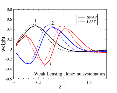
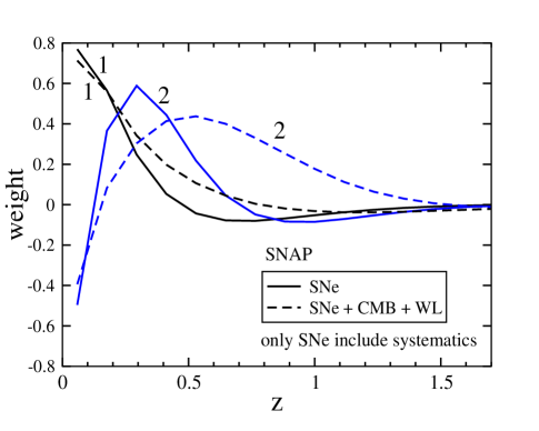
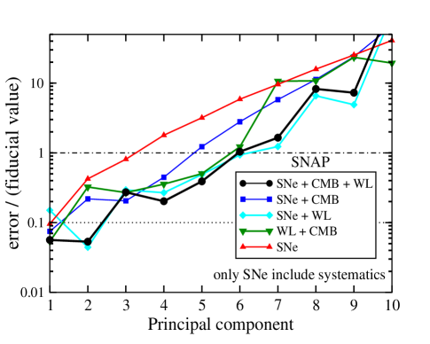
Figure 1: Top left: three best measured principal components of $w(z)$ for the upcoming weak lensing surveys; higher depth and galaxy density (SNAP) and wider area (LSST) each contribute well. Note that the best measured mode peaks at $z\sim 0.4$. Top right: Two of the best measured PCs of $w(z)$ expected for a SNAP-type survey for SN alone, and SN combined with weak lensing and CMB (Planck $d_{A}(z_{\rm lss})$). The best PC from SN alone peaks at $z\sim 0$; this becomes $z\sim 0.2$, if $\Omega_{M}$ is independently known to better than 0.01 (not shown). Note that the second best measured PC is pushed out to higher redshift once the WL and CMB information is added in. Bottom: inverse signal-to-noise in measuring the PCs of $w(z)$; that is, accuracies in measuring the PC coefficients divided by their fiducial values. We show the cases of SN alone, SN+CMB, SN+WL, WL+CMB, and the three probes combined. Throughout, we include the systematics in SN constraints, but not in WL estimates as the systematics contributions to the latter are highly uncertain.

The top left panel in Fig. 1 shows the three best measured principal components of $w(z)$ for weak lensing SNAP and LSST surveys. Note that the best measured PC peaks at $z\sim 0.4$ – as expected, the sensitivity of weak lensing surveys to dark energy is at higher redshifts than that of SN, which are shown in the top right panel. We also see that while adding the WL+CMB information does not drastically change the shape of the best SN PC, the second best-measured PC, and higher ones, are moved to higher redshifts.

The bottom panel of Fig. 1 shows the principal result: the inverse signal-to-noise in measurements of each PC for SN alone, SN+CMB, SN+WL, WL+CMB, and the three probes combined. More precisely, we computed the coefficient of each principal component entering the fiducial $w(z)$ and its error, and define $\sigma_{PC}=$error/coefficient. [Note that it is $\sigma_{\rm PC}$, and not the raw error, that matters and determines at how many “sigma” each PC is detected]. To guide the eye we also plot two horizontal lines corresponding to two criteria for parameter measurement accuracy: the weak criterion $\sigma_{\rm PC}=1$ (below which we have a “1-$\sigma$ detection” of a given PC) and the strong criterion $\sigma_{\rm PC}=0.1$ which is precisely equivalent to our 10% criterion from Sec. III.

We see that SN measurements alone, with systematics, measure three PCs to $S/N>1$, and they are further significantly helped by adding the Planck measurement of $d_{A}(z_{\rm lss})$ (cf. frieman ). Weak lensing power spectra alone, without systematics however, measures four PCs to precision satisfying the weak criterion (not shown). Finally, combining all three probes leads to five (nearly six) PCs measured to $S/N>1$. This is quite encouraging and shows in a slightly different light that all three surveys contribute nontrivially to the information content. However, we also find that all three surveys combined lead to only two PCs passing the strong criterion, and two more if we dilute it to 25% precision ($\sigma_{\rm PC}=0.25$). Our results are in rough agreement with those of Knox et al. Knox who also consider the error in measurement of the PCs with both SN and WL. (Note that taking instead LSST-like WL data does not change the numbers of PCs quoted above.)

These results indicate that it is not just a matter of finding a “better” parametrization. Even with allowing $w(a)$ to take on whatever form the data best fit, next generation data can only generically provide tight constraints on two dark energy parameters.

V Conclusion

We have examined various characterizations of the dark energy in both parametric and non-parametric forms. Even with observational data corresponding to next generation probes of supernova distances, weak lensing shear, and the CMB, we find it is extremely challenging to give a model independent description of the equation of state with more than two parameters: the value at some epoch and a measure of its variation. The good news is that the two parameter model in current use is well understood, physically motivated, and accurate.

To some extent this should not be surprising. If the underlying microphysics, e.g. potential of the dark energy field, is reasonably smooth, described by a few parameters, then we should not expect more parameters to be evident in the equation of state. However we note that other microphysics, such as couplings to matter or non-canonical sound speed Hu_GDM ; dedeo , have not been addressed here (although if $w\approx-1$ then we do not expect the sound speed to have much observable effect bean_dore ; weller_lewis ; cor_speed ; hannestad ).

A more fundamental question to ask is what physics would we learn anyway with fitting a third parameter; the physical interpretation of basic dynamical characteristics such as an equation of state value and its variation is clear, but an extra parameter for the sake of having more may not hold much revelation, i.e. no real qualitative difference. Furthermore, if we concatenate all our cosmological probes together in the quest for one more piece of information then we run the risk of losing the ability to test a more general framework. For example, by contrasting the expansion history with the growth history lue_DGP ; lingrav ; lindeal ; knoxtyson , e.g. supernovae and weak lensing separately, we can seek whether the general concept of an effective equation of state $w(a)$ corresponds to the specific origin of a high energy physics scalar field or a modification of Einstein gravity.

More elaborate parametrizations have some uses, e.g. testing for bias in the recovered $w(z)$ (e.g. bassett_compression ) or searching for a particular property (e.g. rapid evolution), but this must be weighed against the fact that extra parameters can only be weakly constrained. In fact, even if we reduce a higher parameter model down to two parameters by a physically motivated fixing of some parameters, in most cases the complementarity of all three cosmological probes is essential. The standard parametrization in terms of $w_{0}$ and $w_{a}$ is one of the few successful enough to manage a generic fit with only a subset of probes; another is the new four parameter model introduced, with fixed transition epoch and rapidity.

The principal component decomposition of dark energy equation of state is a powerful approach that explicitly protects against biases in parameter determination and separates the accurately measured parameters from the poorly measured ones. But even the PC method has weaknesses – the recovered principal components depend on the survey specifications, and are not related to fundamental physics of dark energy in any obvious way. Most likely the most powerful approach of characterizing dark energy will be testing the data in multiple ways, through both a parametrized function and PCA to check for consistency.

The conclusion is that more than two parameters is not viable for a general fit with next generation data if we are interested in parameters directly informative about the nature and dynamics of dark energy that do not require further differentiation with respect to redshift. We can then ask how good do we need – what are the requirements on the data such that we would be successful in characterizing the dark energy dynamics with a third parameter. For the power law extension, Model 3.1, to estimate $b$ to 0.2 (with a fiducial SUGRA model), we require next-next generation improvements in all three probes together. Next-next generation experiments are defined as those that determine the distances for $z=0-1.7$ to 0.05%, averaged over redshift bins $\Delta z=0.1$, weak lensing shear power spectrum at the level equivalent to that of a completely systematics free survey with 10000 square degrees and 100 galaxies per square arcminute, and the CMB distance to last scattering to 0.1%. For the cubic case, Model 3.2, the requirement is next-next generation accuracy on either SN+CMB or WL+CMB. For the four parameter dynamics, one can attain successful fits to all four parameters with either next-next generation improvements to SN or to WL. However, this was for the most sensitive fiducial model and does not hold generally. For example, next-next accuracy on all three probes still fails to fit even three parameters if the true model instead possesses, say, $a_{t}=0.3$ or $\tau=1$.

So while it is not clear what we would gain in physics insight from going beyond two parameters, it is apparent that it would be extraordinarily difficult to achieve such characterization. The two basic dynamical properties of the dark energy equation of state value and variation seem a reasonable and realistic goal for the next generation.

References

- (1) E.V. Linder & A. Jenkins, MNRAS 346, 573 (2003) [astro-ph/0305286]
- (2) U. Alam, V. Sahni, T.D. Saini, A. Starobinsky, MNRAS 344, 1057 (2003) [astro-ph/0303009]
- (3) R.R. Caldwell & E.V. Linder, astro-ph/0505xxx
- (4) E.V. Linder, Phys. Rev. Lett. 90, 091301 (2003) [astro-ph/0208512]
- (5) E.V. Linder, Phys. Rev. D 70, 023511 (2004) [astro-ph/0402503]
- (6) P.-S. Corasaniti & E.J. Copeland, Phys. Rev. D 67, 063521 (2003) [astro-ph/0205544]
- (7) B.A. Bassett, M. Kunz, J. Silk, C. Ungarelli, MNRAS 336, 1217 (2002) [astro-ph/0203383]
- (8) E.V. Linder & R. Miquel, Phys. Rev. D 70, 123516 (2004) [astro-ph/0409411]
- (9) D. Rapetti, S.W. Allen, J. Weller, MNRAS accepted [astro-ph/0409574]
- (10) E.V. Linder, in draft (2005)
-
(11)
SNAP – http://snap.lbl.gov ;
Aldering, G. et al. 2004, PASP, submitted [astro-ph/0405232] - (12) A. Refregier et al., Astron. J. 127, 3102 (2004) [astro-ph/0304419]
- (13) D.J. Eisenstein, W. Hu and M. Tegmark, Astrophys. J., 518, 2 (1999)
- (14) D.J. Eisenstein & W. Hu, Astrophys. J., 511, 5 (1999)
- (15) R.E. Smith et al., MNRAS, 341, 1311 (2003)
- (16) D. Huterer, M. Takada, G. Bernstein & B. Jain, in draft (2005)
- (17) J.A. Frieman, D. Huterer, E.V. Linder and M. Turner, Phys. Rev. D, 67, 083505 (2003)
- (18) P.S. Corasaniti, M. Kunz, D. Parkinson, E.J. Copeland and B. Bassett, Phys. Rev. D 70, 093006 (2004)
- (19) A. Cooray & D. Huterer, Astrophys. J., 513, L95 (1999)
- (20) D. Huterer & M.S. Turner, Phys. Rev. D 64, 123527 (2001)
- (21) D. Huterer & G. Starkman, Phys. Rev. Lett., 90, 031301 (2002)
- (22) L. Knox, A. Albrecht and Y.-S. Song, Proceedings of NOAO Workshop on Observing Dark Energy [astro-ph/0408141]
- (23) W. Hu, Astrophys. J., 506, 485 (1998)
- (24) S. DeDeo, R.R. Caldwell and P.J. Steinhardt, Phys. Rev. D, 67. 103509 (2003)
- (25) R. Bean and O. Dore, Phys. Rev. D, 69, 083503 (2004)
- (26) J. Weller and A.M. Lewis, MNRAS, 346, 987 (2003)
- (27) P.S. Corasaniti, T. Giannantonio and A. Melchiorri, astro-ph/0504115
- (28) S. Hannestad, astro-ph/0504017
- (29) A. Lue, R. Scoccimarro and G.D. Starkman, Phys. Rev. D, 69, 124015 (2004)
- (30) E.V. Linder, in DARK2004, Proceedings of 5th International Heidelberg Conference (2004) [astro-ph/0501057]
- (31) L. Knox, Y.-S. Song and J.A. Tyson, astro-ph/0503644
- (32) B. Bassett, P.S. Corasaniti and M. Kunz, Astrophys. J., 617, L1 (2004)