Development of Kolmogorov spectrum in the pulsar radio emission
Abstract
It is shown that the scattering of electromagnetic waves by Langmuir ones taking into the account the electric drift motion of particles, is the most intense nonlinear process and should be responsible for the formation of radiation spectrum of radio pulsars. Performed analysis indicates that in the case of existence of inertial interval formation of stationary spectra is possible. Analysis of linear mechanisms of wave generation and silk allow to conclude that only possible stationary solution has spectral index . Obtained spectrum is in good agreement with observational data.
pacs:
97.60.Gb, 52.35.RaI Introduction
Aim of the present work is to study nonlinear processes responsible for the formation of the radio emission spectrum in the pulsar magnetosphere. The spectra of pulsar radio emission has been intensively studied by observers M96 ; MKKW00 ; LYLG95 ; IKMS81 ; LSG71 . Above 100 MHz observed intensity of the majority of pulsars can be described by a simple power law with average value of spectral index MKKW00 . Spectral index of individual pulsars vary from to . Some pulsars has the spectra which can be modelled by the two power law M96 ; LYLG95 , but it seems that single power law is a rule and the two power law spectrum is a rather rare exception MKKW00 .
From our point of view pulsar radio emission is generated and formed in the magnetosphere. Therefore properties of the radiation is mainly determined by the physical processes in the magnetosphere plasma. This approach allows to explain other main characteristics of pulsar radiation, such as polarization properties KMM91 , nullings KMMS96 , micro impulses KMMS01 , mode switching MMMM97 and so on.
In the presented paper we study nonlinear processes in the magnetosphere plasma that should be responsible for the formation of the pulsar radio emission spectra. Mathematical methods used for analysis is based on the weak turbulence theory (see, e.g., ZK78 ; ZLF ).
The paper is organized as follows: the model of the magnetosphere as well as linear eigenmodes of plasma and linear mechanisms of their generation is discussed in Sec. 2. Nonlinear processes are studied in Sec. 3. In Sec 4 stationary solutions fot the spectra are obtained and analyzed.
II Linear modes and their generation in pulsar magnetosphere
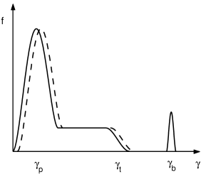
According to the standard model of the pulsar magnetosphere GJ69 ; S71 relativistic plasma that is pierced by electron beam moves along open field lines of pulsar magnetic field . Magnetic field of pulsar is supposed to be dipole. Under open field lines we mean the field lines that crosses the surface of light cylinder - the surface where the velocity of field line solid rotation reaches the speed of light . It is supposed that electric field directed along the open field lines is generated at the surface of pulsar GJ69 , that pulls out electrons of the primary beam from the surface of the star. The particles moving along magnetic field lines generate rays, which on its turn if the energy generate electron-positron pairs S71 . This process is stopped when the initial electric field becomes screened. The particle distribution function that has the form presented in Fig. 1 can be presented as:
| (1) |
where describes the bulk of the plasma, is the distribution function of elongated to the plasma motion tail particles and corresponds to the particles of the primary beam. The distribution function (1) is one dimensional. In Fig. 1 solid and dashed lines correspond to electrons and positrons respectively. The shift of the distribution functions is caused by the existence of the primary beam. It is supposed that
| (2) |
where , are Lorentz factors and , concentrations of bulk, tail and beam particles respectively. For typical pulsars , , , , . Index indicates that the values belong to the surface of the pulsar.
The condition of quasi neutrality yields
| (3) |
here indexes are related to positrons and electrons respectively. are normalized such that .
In spite of the fact that this small difference plays important role in explanation of polarization properties of pulsar radiation. The radiation of the most pulsars has considerable part of circularly polarized radiation. It was shown KMM91 that circular polarization can occur only in small angle between wave veqtor and :
| (4) |
Consequently, the observer receives the radiation that is formed in small angle with respect to . So, for pulsar radio emission the waves propagating nearly along the magnetic field are important. This agrees with linear theory of plasma in strong magnetic field: analysis provides that the wave generation takes place only almost along the magnetic field KMM91 ; VKM85 .
Due to the absence of gyrotropy the spectra of linear modes in plasma is meager. There exist only three modes VKM85 : purely transversal mode and in general partially potential modes. Electric vector of mode is perpendicular to both and . If the dispersion relation of this mode is:
| (5) |
where , and , are plasma and cyclotron frequencies respectively
| (6) |
angular brackets denote averaging over distribution function and .
mode has two branches and . Electric vectors of these modes are located in the plane formed by and . If mode merges with mode with spectrum (5). The mode propagating along is longitudinal Langmuir wave . If their dispersion is S60 ; TS61 :
| (7) |
and when :
| (8) |
where and .
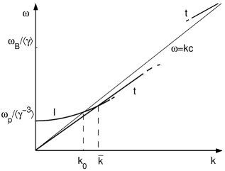
From Eqs. (5) and (8) it follows that frequencies of and modes become equal at:
| (9) |
Dispersion relations of the waves propagating along are presented in Fig. 2.
Mechanisms of wave generation in the magnetosphere plasma has been intensively studied (see, e.g., M86 ). The magnetosphere plasma can be unstable due to two reasons: a) existence of energetic beam; b) absence of symmetry and one dimensionality of the distribution function. Detailed analysis provides KMM91 that the beam instability can develop only due to the drift of the particles in the curved magnetic field (so called ”drift-cherenkov” resonance). Linear stage of this instability was studied in LMB99 and nonlinear stage in SMMK03 . In this paper we will be interested in the second mechanism of instability - excitation at the anomalous Doppler-effect resonance. The condition of this resonance is KMM91 :
| (10) |
Here and are projections of wave vector along and perpendicular to , is curvature drift velocity, is curvature radius of magnetic field lines and is Lorentz factor of resonant particles.
Detailed analysis provides that this condition can be satisfied only for energetic particles of the tale and beam LMM79 , when the condition is satisfied. Substituting Eq. (2) into (10), for we obtain:
| (11) |
From this equation for typical pulsar parameters MU79 ; MU89 it follows that the frequencies of generated waves
| (12) |
It should be noted that transversal waves are strongly damped by cyclotron damping with the bulk particles. The condition of this resonance yields
| (13) |
This condition provides that cyclotron damping is effective for the waves with frequencies
| (14) |
Linear mechanisms of the wave generation discussed in this section emerges transversal waves. On its turn, nonlinear interactions of waves redistributes the energy among different modes and scales and as it will be shown bellow can lead to the formation of stationary spectra of wave turbulence.
III Nonlinear processes
For the development of weak turbulence theory the small parameter of weak turbulence is used. In the case of plasma this parameter is
| (15) |
where is electric vector of the wave. This condition implies that we consider the state when the energy density of plasma is much greater then the energy density of waves. except the parameter (15) in the magnetosphere plasma there exist another two small parameters that greatly simplify future analysis. The first small parameter is . The second one:
| (16) |
allows us to use so-called drift approximation TS .
As it is well known GS if turbulence is weak the dynamics is governed by three wave resonant processes. In plasma there exists additional limitations for realization of three wave resonant interactions. The absence of girotropy causes the fact that the terms proportional to the odd power of the charge do not contribute to the nonlinear currents. Another specific property of the magnetosphere plasma is that all the waves are propagating almost along the magnetic field.
Breakup of wave into two waves was studied in M80 , and all possible three wave processes in GM83 . In this researches main attention was payed to possible breakup of waves because it was believed that these waves should be the most unstable ones. Existence of the anomalous Doppler-effect resonance discussed in the previous Section leads to the conclusion that in fact the most interesting three wave processes are possible breakups of waves that should be responsible for the formation of observed spectra of pulsars.
For the analysis of nonlinear processes it is useful to introduce quantities and notations used in quantum physics. Usually plasmon occupation numbers and wave amplitudes are introduced ZLF ; TS ; GS :
| (17) |
here
| (18) |
is polarization vector of mode; ; is dielectric tensor; denotes complex conjugation and angular brackets denote averaging over phases.
Maxwell equations yield
| (21) |
where matrix element of the process
| (24) |
and is nonlinear conductivity tensor.
If , the process is forbidden due to the fact that the second order current . When , this process can take place but the matrix element of interaction is negligibly small GM83 : .
Another possible three wave process was discussed in GM83 without taking into consideration drift motion of the particles. In this case the frequency of generated Langmuir waves . If all the waves are propagating along , matrix element of interaction is
| (25) |
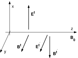
Consideration of the drift motion of particles makes this process even more intense. For simplicity let us consider the case when the waves are propagating along . Let us assume that electric vectors of and waves are directed along and axes respectively (see Fig. 3) and is parallel to axis. causes the drift motion of particles along :
| (26) |
which on its turn generates nonlinear electric field:
| (27) |
It has to be noted that drift velocity is the same for electrons and positrons. Consequently the drift motion do not lead to current generation in the linear approximation. If the resonant conditions
| (28) |
are fulfilled the beating of and waves that generates longitudinal electric field (27) are in resonance with corresponding wave.
Analysis of the resonant conditions (28) yields that wave should have phase velocity a bit less then the speed of light. But this king of waves in general can be strongly damped by collisionless Landau damping. In this case instead of three wave nonlinear interaction one has to consider scattering of waves by plasma particles - so called wave-particle-wave interaction GS ; TS .
Analysis of standard pulsar parameters yield that in principle both cases are possible. In this paper we consider the case when waves involved in resonance with waves are not strongly damped by collisionless damping.
Maxwell equations governing the dynamics in the case when all the waves are propagating along yield:
| (29) |
| (30) |
Nonlinear currents can be readily calculated as follows: substituting (26) into Eq. (27) and taking into account Faraday law we get:
| (31) |
For we have
| (32) |
where perturbation of charge density can be determined from Poisson equation.
Substituting in Eqs. (29)-(30) electric field components as
| (33) |
and taking into account Eqs. (31)-(32) as well as dispersions (5) and (8) we obtain for slowly varying amplitudes:
| (34) |
| (35) |
| (36) |
Assuming that there exist many waves with chaotic phases and introducing occupation numbers:
| (37) |
and using standard technique TS ; GS we get for the matrix element of interaction:
| (38) |
Comparison of Eqs. (25) and (38) yields that the drift motion of particles leads to important intensification of the considered process.
IV Stationary spectra
In the case under consideration . Consequently, the nonlinear interaction is local - only the waves with close frequencies can effectively interact. As it was discussed in Sec. 2 the generation of waves takes place for , whereas the cyclotron damping is effective for . Nonlinear processes are responsible for the formation of stationary spectrum between these intervals of generation and silk. As it is known ZK78 the stationary spectrum in the Kolmogorov interval is fully determined by the matrix element (38) and linear dispersions of waves. There exist two stationary solutions:
| (39) |
where is the dimension of the problem and is the index of homogeneity of the matrix element. The first solution corresponds to constant flux of energy to the smaller scales, whereas corresponds to constant flux of plasmons to the larger scales ZLF ; ZK78 .
In our case and . Therefore and . Taking into account the linear character of wave dispersion for the energy spectrum that is proportional to the observed intensity we have
| (40) |
which of this spectra is realized in practice depends on the linear mechanisms of generation and silk of the waves. In the case under consideration the waves with relatively low frequencies are excited at the anomalous doppler-effect resonance and waves with relatively high frequencies are damped at cyclotron resonance. In this case the spectrum is only possible.
As it was mentioned above most of the pulsars has the spectral indexes . Consequently, obtained theoretical result seems to be in good accordance with the observations.
V Summary
Nonlinear three wave processes that can be responsible for the formation of spectra of radio pulsars is considered. Existence of strong magnetic field makes it necessary to take into account electric drift motion of particles. In the framework of the weak turbulence theory possible stationary spectra that can occur in Kolmogorov interval are calculated. Analysis of linear mechanisms of wave generation and silk allows to conclude that only possible spectral index is . Obtained result is in satisfactory accordance with the observational data.
References
- (1) V. M. Malofeev, APS Conf. Ser. 105, 271 (1996).
- (2) O. Maron, J. Kijak, M. Kramer and R. Wielebinski, Astron. Astrophys. 147, 195 (2000).
- (3) D. R. Lorimer, J. A. Yates, A. G. Lyne and M. D. Gould, Mon. Not. R. Astron. Soc. 273, 411 (1995).
- (4) V. A. Izvekova, A. .D. Kuzmin, V. M. Malofeev and Y. Shitov, Astrophys. and Space Science 78, 45 (1981).
- (5) A. G. Lyne, F. G. Smith and D. A. Graham, Mon. Not. R. Astron. Soc. 153, 337 (1971).
- (6) A. Z. Kazbegi, G. .Z. Machabeli and G. I. Melikidze, Mon. Not. R. Astron. Soc. 253, 377 (1991).
- (7) A. Kazbegi, G. Machabeli, G. Melikidze and C. Shukre, Astron. Astrophys. 309, 515 (1996).
- (8) G. Machabeli, D. Khechinashvili, G. Melikidze and D. Shapakidze, Mon. Not. R. Astron. Soc. 327, 984 (2001).
- (9) O. I. Malov, V. M. Malofeev, G. Machabeli and G. Melikidze, Astron. Zh. 74, 303 (1997).
- (10) V. E. Zakharov and E. A. Kuznetsov, Zh. Éksp. Teor. Fiz. 75, 904 (1978);
- (11) V. E. Zakharov, V.S. L’vov and G. Falkovich, Kolmogorov Spectra of Turbulence I (Springer-Verlag, Berlin, 1992).
- (12) P. Goldreich and W. H. Julian, Astrphys. J. 157, 869 (1969).
- (13) P. A. Sturrock, Astrphys. J. 164, 529 (1971).
- (14) A. S. Volokitin, V. V. Krasnosel’skix and G. Z. Machabeli, Fiz. Plazmy 11, 531 (1985).
- (15) V. P. Silin, Zh. Éksp. Teor. Fiz. 38, 1577 (1960).
- (16) V. N. Tsitovich, Zh. Éksp. Teor. Fiz. 40, 1775 (1961).
- (17) D. B. Melrose, Instabilities in Space and Laboratory Plasmas (Cambridge University Press, 1986).
- (18) V. L. Ginzburg and V. V. Zhelezniakov, Annu. Rev. Astron. Astrophys. 13, 511 (1975).
- (19) M. Lutikov, G. Machabeli and R. Blandford, Astrophys. J., 512, 804 (1999).
- (20) D. Shapakidze, G. Machabeli, G. Melikidze and D. Khechinashvili, Phys. Rev. E, 67, 345 (2003).
- (21) J. G. Lominadze, A. B. Mikhailovski and G. Z. Machabeli, Fiz. Plazmy 5, 748 (1979).
- (22) G. Z. Machabeli and V. V. Usov, Astron. Zh. Lett. 5, 238 (1979).
- (23) G. Z. Machabeli and V. V. Usov, Astron. Zh. Lett. 15, 393 (1989).
- (24) V. N. Tsitovich, Nonlinear Effects in Plasma (Plenum, New Yourk, 1970).
- (25) R. Z. Sagdeev and A. A. Galeev, Nonlinear Plasma Theory (Benjamin, New Yourk, 1969).
- (26) A. B. Mikhailovski, Fiz. Plazmy 6, 613 (1980).
- (27) M. E. Gedalin and G. Z. Machabeli, Fiz. Plazmy 9, 1015 (1983).