The imprints of local superclusters on the Sunyaev-Zel’dovich signals and their detectability with Planck

Abstract

We use high-resolution hydrodynamical simulations of large-scale structure formation to study the imprints of the local superclusters onto the full-sky Sunyaev-Zel’dovich (SZ) signals. Following Mathis et al. (2002), the initial conditions have been statistically constrained to reproduce the density field within a sphere of 110 Mpc around the Milky Way, as observed in the IRAS 1.2-Jy all-sky redshift survey. As a result, the positions and masses of prominent galaxy clusters and superclusters in our simulations coincide closely with their real counterparts in the local universe. We present the results of two different runs, one with adiabatic gas physics only, and one also including cooling, star formation and feedback. By analysing the full-sky maps for the thermal and kinetic SZ signals extracted from these simulations, we find that for multipoles with $\ell<100$ the power spectrum is dominated by the prominent local superclusters, and its amplitude at these scales is a factor of two higher than that obtained from unconstrained simulations; at lower multipoles ($\ell<20$) this factor can even reach one order of magnitude. We check the influence of the SZ effect from local superclusters on the cosmic microwave background (CMB) power spectrum at small multipoles and find it negligible and with no signs of quadrupole-octopole alignment. However, performing simulations of the CMB radiation including the experimental noise at the frequencies which will be observed by the Planck satellite, we find results suggesting that an estimate of the SZ power spectrum at large scales can be extracted.

1 Introduction

It is well known that high-accuracy measurements of the anisotropies of the cosmic microwave background (CMB) are extremely important for cosmology. By analysing their angular power spectrum, $C(\ell)$, it is in fact possible to obtain tight constraints on the mechanisms from which the primordial fluctuations originate and on the main cosmological parameters (or combinations of them) like the matter density, the baryonic density and the cosmological constant contribution. For this reason, the astronomical community has been doing a big effort over the last years in order to improve the quality of the CMB data, both in terms of accuracy and resolution.

The best available CMB measurements up to now were provided by the Wilkinson Microwave Anisotropy Probe satellite (WMAP; Bennett et al., 2003). The data obtained in its first year of activity gave strong support to the so-called concordance model, i.e. a spatially flat universe dominated by dark energy and cold dark matter, with nearly scale-invariant primordial fluctuations, almost gaussianly distributed. The WMAP result is confirming the general picture emerging by the analysis of other different datasets, like high-redshift supernovae Ia, weak lensing, galaxy survey, Lyman-$\alpha$ forest and galaxy clusters (see discussion in Spergel et al., 2003, and references therein).

The statistical analysis and the theoretical interpretation of CMB data of so high quality necessarily require a good understanding of all possible sources of contamination as well as the techniques to separate them from the CMB signal. The Sunyaev-Zel’dovich (SZ) effect (Sunyaev & Zeldovich, 1972), i.e. the Compton scatter of the cold CMB photons by the hot electrons mainly located in the intracluster plasma, certainly represents one of the most important secondary anisotropies, i.e. temperature fluctuations generated along the light trajectory from the last scattering surface to the observer. Different studies have been devoted to the estimate of the SZ angular power spectrum which originates from the whole galaxy cluster population (see, e.g., Cooray et al., 2004, and references therein). The results show that the SZ signal starts to dominate the cosmological one only on very small angular scales ($\ell>2000$), while at the scales covered by WMAP is approximately 3 orders of magnitude smaller.

Even if its amplitude appears relatively small, the SZ signal could be nevertheless significant at the sky positions corresponding to nearby galaxy clusters. This has motivated the research of SZ imprints in the first-year WMAP temperature maps. This approach, mainly based on the cross-correlation of the CMB maps with the observed distribution of clusters and superclusters, as extracted in both optical and X-ray surveys, led to different claims for a positive detection at small angular scales (Myers et al., 2004; Hernández-Monteagudo et al., 2004; Fosalba & Gaztañaga, 2004; Afshordi et al., 2004), but only upper limits for the detection of the SZ signal exist at larger scales at present (Diego et al., 2003; Hernandez-Monteagudo et al., 2004; Hirata et al., 2004; Huffenberger et al., 2004; Hansen et al., 2005). In this sense the situation will largely improve in the near future thanks to the capabilities of the Planck satellite, whose launch is planned for 2007. In fact the range of frequencies covered by its receivers will be very large, and the noise level is expected to be very low. This will allow to extract the SZ signal for at least 10,000 objects out to redshfit $z\approx 1$ (see, e.g. Bartelmann, 2001).

The CMB data from the WMAP satellite exhibit several anomalies at the lowest multipoles, among them the abnormally low value of the quadrupole amplitude (see, however, Efstathiou, 2004) and the fact that the directions of the quadrupole and octopole are unusually well aligned (see, e.g., Gaztañaga et al., 2003; de Oliveira-Costa et al., 2004). There have been some speculation about the possibility that the SZ signal from structures in the local universe (the so-called local supercluster) could be the cause of the low quadrupole (Abramo & Sodre, 2003). Further, the quadrupole and octopole directions happen to be pointing toward the Virgo cluster (de Oliveira-Costa et al., 2004), which opens the possibility of contamination from the local universe.

The goal of this paper is to investigate the importance of the thermal and kinetic SZ effects produced by the local superclusters by comparing it with respect to the cosmological signal and to the contribution of more distant clusters. At this aim we will use the results of high-resolution hydrodynamical simulations realized starting from initial conditions (Mathis et al., 2002) which are constrained to reproduce the density field recovered by the IRAS 1.2-Jy all-sky redshift survey. Using full-sky maps extracted from these numerical simulations, we will discuss the statistical properties of low multipoles in terms of amplitude and alignment. Moreover, taking advantage of the different set of physical processes treated in the simulations we can assess the uncertainties related to the modelization. Finally we will perform simulations to discuss if the local SZ signal can be detected exploiting the capabilities of the Planck satellite.

The plan of the paper is as follows. In Section 2 we describe the general characteristics of the constrained hydrodynamical simulations of the local universe used in the following analysis. Section 3 presents our method to produce full-sky maps of the thermal and kinetic SZ effects. Section 4 is devoted to the results of our analysis. In particular we show the statistical properties of the maps in terms of angular power spectra and alignment of lower multipoles and we discuss the possibility of detecting the local SZ signal with future experiments, like the upcoming Planck satellite. Finally we summarize our findings and draw the main conclusions in the final Section 5.

2 The constrained hydrodynamical simulations

The results presented in this paper have been obtained by using the final output of two different cosmological hydrodynamical simulations of the local universe obtained starting from the same initial conditions but following a different set of physical processes. In more detail we used initial conditions similar to those adopted by Mathis et al. (2002) in their study (based on a pure N-body simulation) of structure formation in the local universe. The galaxy distribution in the IRAS 1.2-Jy galaxy survey is first gaussianly smoothed on a scale of 7 Mpc and then linearly evolved back in time up to $z=50$ following the method proposed by Kolatt et al. (1996). The resulting field is then used as a Gaussian constraint (Hoffman & Ribak, 1991) for an otherwise random realization of a flat $\Lambda$CDM model, for which we assume a present matter density parameter $\Omega_{0m}=0.3$, a Hubble constant $H_{0}=70$ km/s/Mpc and a r.m.s. density fluctuation $\sigma_{8}=0.9$. The volume that is constrained by the observational data covers a sphere of radius $\sim 110$ Mpc, centred on the Milky Way. This region is sampled with more than 50 million high-resolution dark matter particles and is embedded in a periodic box of $\sim 343$ Mpc on a side. The region outside the constrained volume is filled with nearly 7 million low-resolution dark matter particles, allowing a good coverage of long-range gravitational tidal forces.

The statistical analysis made by Mathis et al. (2002) demonstrated that the evolved state of these initial conditions provides a good match to the large-scale structure observed in the local universe. Using semi-analytic models of galaxy formation built on top of merging history trees extracted from the dark matter distribution in the simulation, they showed that the density and velocity maps obtained from synthetic mock galaxy catalogues have characteristics very similar to their observational counterparts. Moreover many of the most prominent nearby galaxy clusters like Virgo, Coma, Pisces-Perseus and Hydra-Centaurus, can be identified directly with haloes in the simulation, with a good agreement for sky positions and virial masses. In fact the positions of all identified objects differ less than the smoothing radius adopted in the initial conditions (7 Mpc), with the only exception of Centaurus, which is displaced by 9.6 Mpc. The agreement for the masses is within a factor of 2 which can be considered acceptable if one considers the uncertainties in the inferred observational masses, mainly when velocity dispersion is used.

Unlike in the original simulation made by Mathis et al. (2002), where only the dark matter component is evolved, here we want to follow also the gas distribution. For this reason we extended the initial conditions by splitting the original high-resolution dark matter particles into gas and dark matter particles having masses of $0.48\times 10^{9}\;M_{\odot}$ and $3.1\times 10^{9}\;M_{\odot}$, respectively; this corresponds to a cosmological baryon fraction of 13 per cent. The total number of particles within the simulation is then slightly more than 108 million and the most massive clusters will be resolved by almost one million particles.

Our runs have been carried out with GADGET-2 (Springel, 2005), a new version of the parallel Tree-SPH simulation code GADGET (Springel et al., 2001). The code uses an entropy-conserving formulation of SPH (Springel & Hernquist, 2002), and allows a treatment of radiative cooling, heating by a UV background, and star formation and feedback processes. The latter is based on a sub-resolution model for the multiphase structure of the interstellar medium (Springel & Hernquist, 2003). The code can also follow the pattern of metal production from the past history of cosmic star formation (Tornatore et al., 2004). This is done by computing the contributions from both Type-II and Type-Ia supernovae and energy feedback and metals are released gradually in time, accordingly to the appropriate lifetimes of the different stellar populations. This treatment also includes in a self-consistent way the dependence of the gas cooling on the local metallicity.

As said, the results presented in this work are based on two different simulations starting from the same initial conditions. The first one, hereafter called gas, includes only non-radiative (i.e. adiabatic) hydrodynamics and has been originally analyzed by Dolag et al. (2005) to study the propagation of cosmic rays in the local universe. Hansen et al. (2005) used the gas properties extracted from this simulation to infer a prediction of the SZ effect from diffuse hot gas in the local universe. In that paper, the PSCz catalogue was used to map the matter density whereas the simulation was used only to assign a temperature for the gas with a given density. The SZ map realized in this way was cross-correlated to the WMAP data and upper limits were found. The second run, hereafter called csf, exploits all the capabilities of the present version of the GADGET code, including cooling, star formation, feedback and metallicity; its outputs will be also used to study the detectability of the diffuse, warm intergalactic medium with future X-ray experiments (Kawahara et al. in preparation).

The feedback scheme for the csf run assumes a Salpeter IMF (Salpeter, 1955) and its parameters have been fixed to get a wind velocity of $\approx 480$ km/s. In a typical massive cluster the SNe (II and Ia) add to the ICM as feedback $\approx 2$keV per particle in an Hubble time (assuming a cosmological mixture of H and He); $\approx 25$ per cent of this energy goes into winds. Note that these values can be considered an upper limit because a part of the ICM affected by the star processes could be at the present time out of the cluster virial radius. Moreover such feedback mechanisms cannot avoid the overcooling problem, commonly found in cosmological simulations: the corresponding overproduction of stars, acting mainly in the central regions, tends to amplify by a factor of $\approx 2$ the effects of the star population. Notice that the metal-dependence of the cooling function does not significantly change the global feedback properties. Another signature that the feedback scheme is not enough efficient is the large amount of metals which is still locked inside the star particles: as a consequence, the resulting ICM metallicity is low, even if still compatible with observed values. A more detailed discussion of cluster properties and metal distribution within the ICM as resulting in simulations including the metal enrichment feedback scheme can be found in Tornatore et al. (2004).

The gravitational force resolution (i.e. the comoving softening length) of both simulations has been fixed to be 14 kpc (Plummer-equivalent), which is comparable to the interparticle separation reached by the SPH particles in the dense centres of our simulated galaxy clusters.

In Table 1 we report the main characteristics of the most prominent clusters in our simulations. In particular, we computed the (mass-weighted) temperature within one tenth of the virial radius, and the central Compton-$y$ parameter. In agreement with previous results in the literature (see, e.g., Tornatore et al., 2003), we find that the temperatures for a given object in the ${\it csf}$ simulation are always larger than in the ${\it gas}$ simulation by a factor of approximately 15-20 per cent. Including radiative cooling causes in fact a lack of pressure support, with a subsequent heating of the infalling gas by adiabatic compression. The opposite trend is present for the central Compton-$y$ parameter, which can be larger by a factor up to 2 in the ${\it gas}$ simulation than in the ${\it csf}$ one (see also White et al., 2002; da Silva et al., 2004; Motl et al., 2005). For completeness, we also list the available observational estimates, which are in rough agreement. Notice that only for Coma we averaged in the simulation the value for Compton-$y$ within an area of 450 kpc to be compatible with the beam size of the observational data (Battistelli et al., 2003). Finally we would like to remark that the observed temperatures are not directly comparable with the simulation results, because they are extracted from X-ray spectroscopic data: as shown by Mazzotta et al. (2004) (see also Rasia et al., 2005; Vikhlinin, 2005), there could be a significant bias produced by the complexity of the thermal structure. For completeness we added in the table the values for the spectroscopic-like temperature $T^{\rm SL}$, which approximates the spectroscopic temperature better than few per cent (Mazzotta et al., 2004).

Table 1: Comparison of the properties of the 6 most prominent clusters, listed in Column 1. The observed cluster temperatures $T_{\rm obs}$ (Column 2) are taken from Mohr et al. (1999), with the exception of the data for Virgo (Sanderson et al., 2003) and A3627 (Ikebe et al., 2002). Columns 3 and 5 refer to the mass-weighted temperature within $0.1\times R_{\rm vir}$, as computed in the gas and csf simulations ($T_{\rm gas}^{\rm MW}$ and $T_{\rm csf}^{\rm MW}$, respectively). Columns 4 and 6 refer to the spectroscopic-like temperature (Mazzotta et al., 2004) within $0.1\times R_{\rm vir}$, as computed in the gas and csf simulations ($T_{\rm gas}^{\rm SL}$ and $T_{\rm csf}^{\rm SL}$, respectively). In Column 7 we report the value for the Compton-$y$ parameter, as obtained for Coma by Battistelli et al. (2003). Columns 8 and 9 refer to the values for $y$ computed in the gas and csf simulations ($y_{\rm gas}$ and $y_{\rm csf}$, respectively). For Coma we averaged the Compton-$y$ within an area of 450 kpc to be compatible with the beam size of the observational data (Battistelli et al., 2003).

Cluster	$T_{\rm obs}[\rm kev]$	$T_{\rm gas}^{\rm MW}[\rm kev]$	$T_{\rm gas}^{\rm SL}[\rm kev]$	$T_{\rm csf}^{\rm MW}[\rm kev]$	$T_{\rm csf}^{\rm SL}[\rm kev]$	$y_{\rm obs}[10^{-5}]$	$y_{\rm gas}[10^{-5}]$	$y_{\rm csf}[10^{-5}]$
Coma	$8.21^{+0.16}_{-0.16}$	6.1	5.8	7.3	7.3	$9.6^{+1.1}_{-1.1}$	9.2	6.4
Virgo	$2.55^{+0.07}_{-0.06}$	3.5	3.0	4.1	3.5		4.8	3.1
Centaurus	$3.54^{+0.08}_{-0.08}$	3.8	3.6	4.6	4.5		6.7	4.2
Hydra	$3.10^{+0.11}_{-0.11}$	3.2	3.2	4.5	4.6		9.3	4.2
Perseus	$6.33^{+0.21}_{-0.18}$	5.8	5.2	6.1	5.8		9.5	6.8
A3627	$5.62^{+0.12}_{-0.11}$	3.7	3.6	4.4	4.4		6.6	4.2

3 Full sky map making

Hot electrons, which are present in the intracluster medium, scatter by inverse Compton the cold photons of the cosmic microwave background (CMB) radiation and re-distribute them towards higher frequencies. The result is the so-called SZ effect (Sunyaev & Zeldovich, 1972) which originates a temperature decrement below 217 GHz, and an increment above.

Given a direction $\vec{\theta}$, the change of the CMB temperature $T_{\rm CMB}$ produced by the thermal SZ effect is given by

$$\frac{\Delta T_{\rm CMB}}{T_{\rm CMB}}=y(\vec{\theta})g(x)\ ,$$ (1)

where $g(x)=x\cdot{\rm{coth}}(x/2)-4$ and $x\equiv h\nu/kT_{\rm CMB}$.

The Compton-$y$ parameter is related to the three-dimensional thermal electron density, $n_{e}$, and to the electron temperature, $T$, by

$$y(\vec{\theta})={{k\sigma_{{}_{T}}}\over{m_{e}c^{2}}}\int{\rm d}l\ n_{e}(\vec{\theta},l)\ T(\vec{\theta},l)\ ,$$ (2)

$\sigma_{{}_{T}}$ being the Thomson scattering cross section.

The kinetic SZ effect is produced by the motion of the intracluster gas with respect to the CMB. The corresponding change of the CMB temperature can be written as

$$\frac{\Delta T_{\rm CMB}}{T_{\rm CMB}}=-w(\vec{\theta})\ ,$$ (3)

with

$$w(\vec{\theta})=\frac{\sigma_{{}_{T}}}{c}\int{\rm d}l\ n_{e}(\vec{\theta},l)\ v_{r}(\vec{\theta},l)\ ,$$ (4)

where $v_{r}$ is the radial component of the cluster velocity.

The line of sight integrals which are present in the definitions of $y$ (eq. 2) and $w$ (eq. 4) can be computed in the simulations by exploiting the SPH kernel. Here we employ the spline kernel defined as (Monaghan & Lattanzio, 1985)

$$W(r/h)=\frac{\pi}{h^{3}}\left\{\begin{array}[]{ll}1-\frac{3}{2}(r/h)^{2}+\frac{3}{4}(r/h)^{3}&0\leq(r/h)\leq 1\\ \frac{1}{4}(2-r/h)^{3}&1\leq(r/h)\leq 2\\ 0&2\leq(r/h)\\ \end{array}\right.,$$ (5)

where $h$ is the so-called SPH smoothing length and $r$ represents the impact parameter. In this way eq.(2) becomes

$$y_{\rm int}=\int\sum_{j}\frac{m_{j}}{\rho_{j}}y_{j}W(d_{j}(r)/h_{j}){\rm d}r\ ,$$ (6)

where $m_{j}$ and $\rho_{j}$ are the mass and density of the $j$-th gas particle, $y_{j}$ is the corresponding Compton $y$-parameter and $d_{j}(r)$ is the projected distance with respect to the position $r$ along the line of sight. A similar relation can be written for $w_{\rm int}$.

In principle the sum has to be done over all particles, but in the case of a compact kernel where $W(r/h)$ gets zero at large $r/h$ (as the one we use) it can be restricted to those particles having a distance from the line of sight smaller than twice their smoothing length.

In practice, however, one would like to obtain the value averaged over all lines of sight crossing the pixel, instead of the value along the line of sight crossing the centre of the pixel only. This can become a problem when the projected size of the structure producing the signal gets smaller than the pixel size. Therefore one usually applies the so called gather approximation, where, given a pixel, all particles - whose projections either overlap or completely fall inside the pixel - are taken into account. In this case the value of the Compton-$y$ parameter can be written as the sum of the contributions of all relevant particles as:

$$y_{\rm pix}=\sum_{j}\frac{m_{j}}{\rho_{j}}y_{j}N_{j}\frac{A_{\rm pix}}{A_{j}}W_{\rm int}(\tilde{d_{j}}/h_{j})\ ,$$ (7)

where $\tilde{d_{j}}$ is the projected distance between the particle and the pixel centre and $W_{\rm int}$ is the integrated kernel. The area $A_{j}$ associated to each gas particle can be approximated as the square of the cubic root of the corresponding volume, i.e. $A_{j}=(m_{j}/\rho_{j})^{2/3}$. The normalization factor $N_{j}$ is given by

$$\sum_{\rm pix}N_{j}A_{\rm pix}W_{\rm int}(\tilde{d_{j}}/h_{j})=A_{j}$$ (8)

to ensure the conservation of the quantity $y$ when distributed over more than one pixel.

The method needs two further corrections. First, for pixels which are only partially overlapped by the projected SPH smoothing kernel, we approximate the associated area $\hat{A}_{\rm pix}$ as

$$\hat{A}_{\rm pix}=\sqrt{A_{\rm pix}}\times(\tilde{d_{j}}+0.5\sqrt{A_{\rm pix}}-h_{j})\ .$$ (9)

To compute the contribution to such a pixel, the weight of the integrated kernel $W_{\rm int}$ is then corrected by a factor $\hat{A}_{\rm pix}/A_{\rm pix}$. This must be taken also into account when normalizing the integrated kernel. We checked that this correction leads to very small changes in the majority of the pixels, but its effect can become substantial in the high-signal regions corresponding to the cluster cores, specially when the particles are distributed over a small number of cells.

Second, when a particle contributes to one pixel only, we fix the integrated kernel $W_{\rm int}$ to be unity. This is important when the area associated to such particle is much smaller than the pixel area and ensures that the value corresponding to the particle is completely given to this pixel: in this case the normalization factor $N_{j}$ can become significantly smaller than unity to ensure the conservation of the quantities. Finally we notice that, since the SZ effect is independent of distance, no distance factor has to be included into the previous equations.

Figure 1 exemplifies the three different situations previously discussed by showing how the gas particles can contribute to one pixel (here represented by the square). In such cases, the weight contributed by particle 1 (shown in red) is $A_{1}/A_{\rm pix}$, the weight for particle 2 (in green) is $W_{\rm int}(r_{2}/h_{2})\hat{A}_{2}/A_{2}$ and the weight for particle 3 (in blue) is $W_{\rm int}(r_{2}/h_{2})A_{\rm pix}/A_{3}$. Note that for particles 2 and 3 the weight needs to be normalised to unity when summed over all pixels to which the particles are contributing.

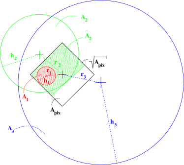
Figure 1: Sketch of three different geometrical situations for particles contributing to one pixel (represented by the black square). Particle 1 (in red), having a smoothing length $h_{1}$ and being at a distance $r_{1}$ from the pixel centre, falls completely inside the pixel, but does not overlap the centre. Particle 2 (in green) covers only partially the pixel. For particle 3 (in blue) the whole pixel lies within its projected radius.

Our maps have been constructed by applying the previous technique directly to the HEALPIx  representation of the full sky (Górski et al., 1998). We fix the nside parameter to be 1024, which results in an all-sky representation with $\approx 1.2\times 10^{7}$ pixels. In order to avoid spurious effects the line of sight integral has been performed between a minimum and maximum distance ($r_{\rm min}$ and $r_{\rm max}$, respectively). In particular we fix $r_{\rm min}=5$ Mpc to be sure that the observer is outside the SPH smoothing radius of all particles, and $r_{\rm max}=110$ Mpc, which represents a conservative limit of our high-resolution region.

4 Results

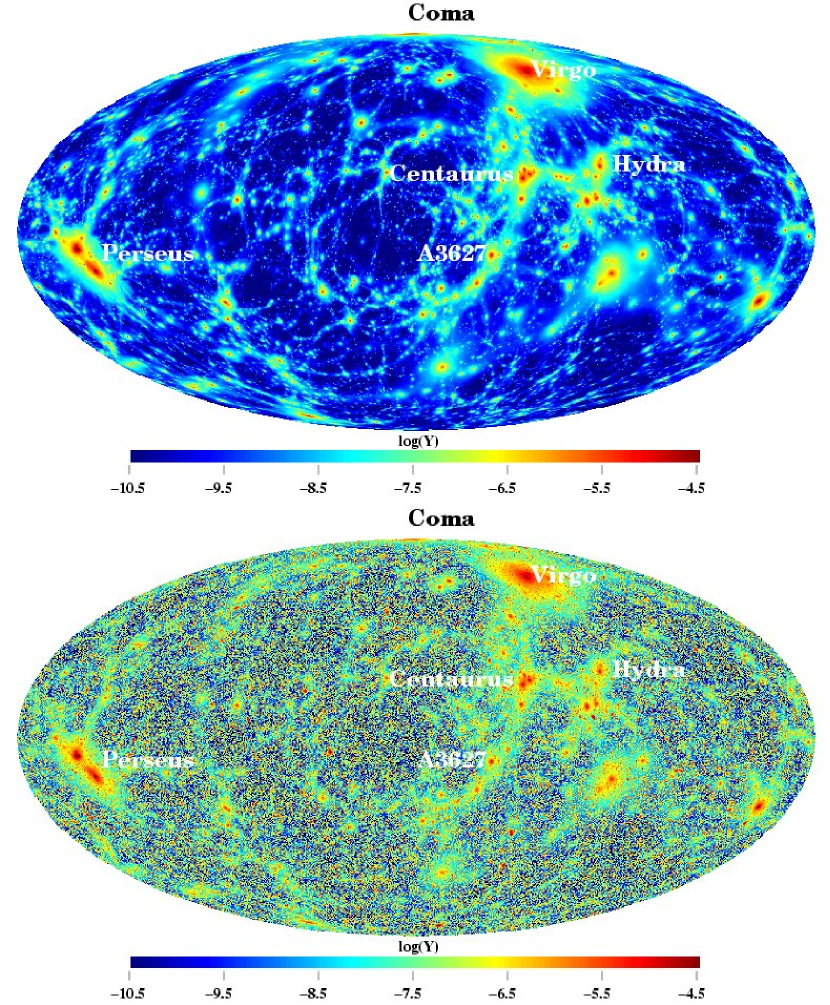
Figure 2: Full-sky map of Compton-$y$ parameter in galactic coordinates. The upper panel shows the results from the gas simulation, covering the local universe up to 110 Mpc from the Milky Way, while in the lower panel we added the contribution from more distant objects, as estimated by Schaefer et al. (2004a). The position of the most prominent structures is indicated in the maps.

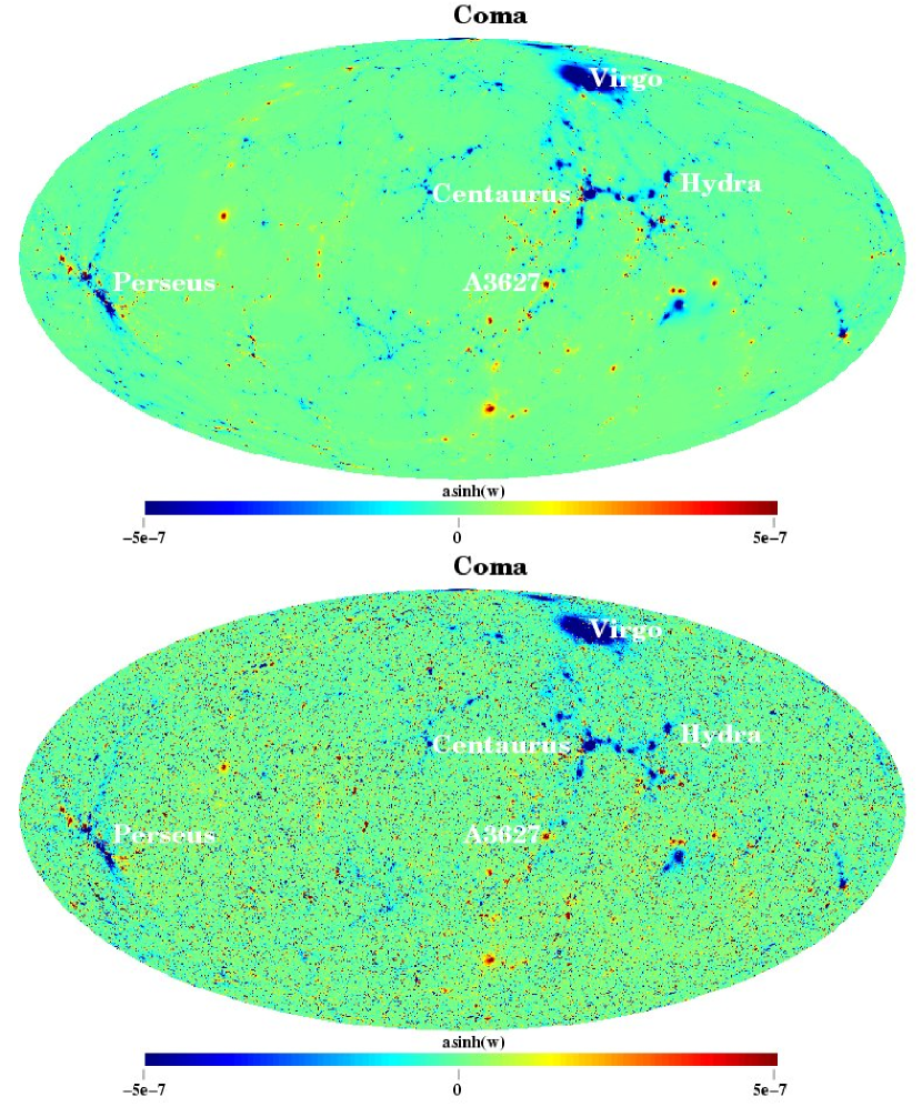
Figure 3: The same as Fig.2, but for the kinetic SZ effect, shown by using ${\rm asinh}(w)$ to better display positive and negative values.

4.1 Full-sky maps

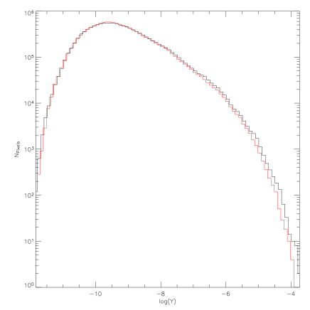
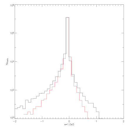
Figure 4: Comparison between the SZ signals as extracted from the gas and csf simulations (black and red lines, respectively). The number of pixels having a given value for the Compton-$y$ parameter and the kinetic parameter $w$ are shown in the left and right panels, respectively.

In Fig. 2 we show the results of the application of the previous method to obtain a full-sky map of the Compton-$y$ parameter in supergalactic coordinates. The upper panel corresponds to the signal resulting from our gas simulation, covering the local universe up to $110$ Mpc. It is possible to recognize the most prominent features: Perseus, Virgo, Centaurus, Hydra, A3627 and Coma (very close to the northern pole of the map). Also the presence of the filamentary structure connecting the largest clusters is still evident. In the lower panel we show the same map where we add the contribution coming from more distant objects. This has been computed by exploiting the results of Schaefer et al. (2004a,b), who build SZ signal maps by using the Hubble volume simulation (Colberg et al., 2000; Jenkins et al., 2001) and suitably inserting the outputs of different hydrodynamic re-simulations of single clusters. Notice that the physical processes considered in these re-simulations, i.e. non-radiative hydrodynamics, are the same included in our gas simulation, so no biases are introduced in combining the results. With respect to the Schaefer et al. (2004) work we add only the objects having a distance from the observer larger than 110 Mpc, because the closer ones are already represented in our simulation. The resulting map appears more patchy, having a significant contribution coming from a large number of distant clusters.

The corresponding maps for the kinetic SZ signal $w$ are shown in Fig. 3. Again the most important structures of the local universe are evident in the upper map and continue to give the dominant contribution in the map including distant objects, shown in lower panel.

It is worth to notice that within the simulation we measure a velocity at the observer’ position of $v_{x}\approx-270$ km/s, $v_{y}\approx 420$ km/s and $v_{z}\approx-350$ km/s (assuming supergalactic coordinates). This leads to a absolute velocity of $v\approx 610$ km/s, which is in good agreement with the observed value (see, e.g., the WMAP analysis by Bennett et al., 2003). Again, the observer’ velocity points toward a direction which differs from the observed one less than 10 degrees: this emphasizes once more that our simulations are giving a good representation of the large-scale structure in our local universe.

By analyzing the maps obtained from the results of the csf simulation (not shown here) we find only small differences with respect to the previous results, mainly in correspondence of the high-density regions, where the cfs simulation tends to give smaller signals. This difference can be quantified by looking to the pixel distribution as a function of $y$ and $w$. This is shown in Fig.4, where the contribution of the local universe only is considered. Concerning the thermal SZ effect (left panel), the histograms are in general very similar, with only a slightly higher frequency for higher values in the gas simulation. The differences are more evident in the pixel distributions for the kinetic parameter $w$: again high (absolute) values have higher probability in the gas simulation than in the csf one.

Analyzing the gas bulk motions, we find no significant difference in the gas and csf runs. Moreover the winds driven by the feedback process are very efficiently stopped short after leaving the star forming region and consequently are not contributing to the kinetic SZ signal. Therefore the difference observed in Fig. 4 reflects the fact that the pressure in the csf simulation is smaller than in the gas one. Again the magnitude of the effect is in good agreement with previous findings (White et al., 2002).

Notice that the distribution for $w$ is clearly non-gaussian, with a more extended tail toward negative values, produced by the cluster motion inside the local universe. Since the spectral signature of the kinetic SZ effect is the same of CMB, a perfect removal of this contribution could be difficult.

It is also worth to notice that the mean value of the Compton-$y$ parameter computed over the whole sky is dominated by the background map extracted from the Hubble volume simulation. For the total map (Fig. 2, lower panel) we get a mean value of $3.3\times 10^{-7}$, whereas we find a much smaller mean value ($4.1\times 10^{-8}$) when considering only the map from the constrained simulation (gas run). As discussed before, this value slightly decreases when using the cfs simulation ($3.2\times 10^{-8}$). Note that all these values are well below the upper limit derived from COBE FIRAS data (Fixsen, 2003).

4.2 The angular power spectrum

In order to quantify the amount of signal produced by the SZ effects, we compute from our maps the angular power spectrum $C(\ell)$. In particular we estimate the spectra in the Rayleigh-Jeans region, where $\Delta T_{\rm CMB}/T_{\rm CMB}=-2y$.

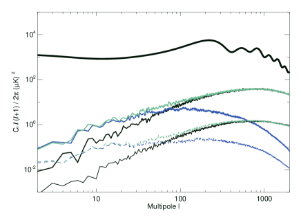
Figure 5: The power spectra for the SZ effects. Comparison between the cosmological CMB power spectrum (upper black solid lined) and the SZ signals obtained in the different simulations: Hubble volume simulation (black lines), local constrained gas simulation (blue lines); local constrained gas simulation combined with the Hubble volume simulation for larger distances (green lines). Upper and lower curves refer to the contributions from thermal and kinetic SZ effects, respectively. All spectra are taken in the Rayleigh-Jeans region where $\Delta T_{\rm CMB}/T_{\rm CMB}=-2y$.

The results are shown in Fig.5, where we compare the power spectrum of the primordial CMB radiation (here represented by the upper black line corresponding to the best fit of the WMAP data obtained by Spergel et al., 2003) to the signals extracted from the numerical simulations here considered. In particular the plot shows $C(\ell)$ for the gas simulation and distinguishes the contributions coming from the local universe from the one produced by more distant galaxy clusters. Both the thermal and kinetic SZ effects are considered. The results confirm that for $\ell<2000$ the cosmological signal is dominating the SZ one, being approximately 3-4 orders of magnitude larger. Moreover the kinetic signal is always smaller by a factor of 10-20 than that produced by the thermal SZ effect. By comparing the results of our simulation with the estimates obtained by Schaefer et al. (2004), who populated the dark matter only Hubble volume simulation (Colberg et al., 2000; Jenkins et al., 2001) with individual, adiabatic cluster simulations, we notice that the SZ effect from the local universe (objects with distance smaller than 110 Mpc from the Milky Way) is the most important contribution up to scales corresponding to $\ell\approx 100$. This is due to the larger angular size of the local supercluster structure. On the contrary, the signal at larger multipoles ($\ell>200$) seems to be dominated by the more distant sources, which are lying outside of our simulated volume.

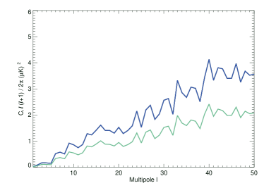
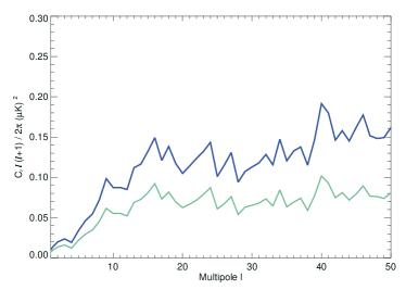
Figure 6: Effects on the power spectra of the inclusion of different physical processes in the constrained simulations of the local universe. Blue and green curves show $C_{l}$ as extracted from the gas and csf simulations, respectively. Upper and lower panels refer to the thermal and kinetic SZ effects, respectively. All spectra are taken in the Rayleigh-Jeans region where $\Delta T_{\rm CMB}/T_{\rm CMB}=-2y$.

In order to quantify the contribution coming from the most prominent clusters, we compute $C(\ell)$ from our maps by applying the galactic cut and masking the regions where the 7 largest local galaxy clusters are located. The resulting power spectrum (not shown here) changes drastically for $\ell>50$ falling off much more rapidly, while remains unchanged for $\ell<50$. This is an expected result, because the richest clusters are contributing to the power around 2-3 degrees, whereas the total signal from all the rest is dominating the large-scale power.

We further checked the contribution from diffuse gas by masking out in the maps the pixels with Compton-$y$ parameter smaller than a given value ($y=10^{-6}$): in such a way only the signal from cluster cores remains. The resulting power spectrum is not strongly affected, showing that the diffuse gas contributes minimally to the observed SZ power. In Fig. 7 we show the power spectrum including and excluding the diffuse gas contribution (solid and dotted lines, respectively) along with the power spectrum extracted from the Hubble volume simulation (dashed line). Note that the Hubble volume simulation gives a lower power spectrum at the largest scales when compared to the constrained simulation, even when the diffuse gas is removed from it.

Figure 7: The large-scale power spectrum of the SZ effect obtained from the constrained simulations including (solid line) and excluding (dotted line) the diffuse gas contribution. The dashed line shows the power spectrum of the Hubble volume simulation.

Having two different constrained realizations of the local universe, the first one with adiabatic physics only, the second one including also cooling, star formation and feedback (the gas and csf simulations, respectively), it is possible to discuss how the previous results depend on the set of the included physical processes. This is done in Fig.6, where we compare directly the power spectra obtained from the two simulations. We find a higher signal in the adiabatic simulation, both for the thermal and kinetic SZ effects. The amplitude of this difference is very similar in both cases, being approximately a factor of 2. This is in agreement with the results obtained from individual cluster simulations (see, e.g., White et al., 2002). Therefore we do not expect the signal to get stronger when including additional physical processes and we can take the results obtained from the gas simulation as a robust upper bound.

4.3 Alignment of lower multipoles

Several anomalies have been detected at low multipoles in the WMAP data. In particular Tegmark et al. (2003) and de Oliveira-Costa et al. (2004) find the CMB quadrupole and octopole to have an unusually high degree of alignment, which is significant at the $2\sigma$ level. Moreover they show that the directions of the quadrupole and the octopole are close to the direction of the Virgo cluster which could suggest a possible link to structures in the local universe. By analysing our SZ templates, we find that the directions of the quadrupole and octopole (shown in Fig. 8 for the gas simulation) are very different from that extracted from the WMAP data: in our maps the quadrupole and octopole point toward $(b,l)\approx(42.3^{\circ},-177.6^{\circ})$ and $(b,l)\approx(32.5^{\circ},88.1^{\circ})$, respectively, while the preferred axes in the WMAP data are in the directions $(b,l)\approx(58.8^{\circ},-102.4^{\circ})$ for the quadrupole and $(b,l)\approx(62.0^{\circ},-121.6^{\circ})$ for the octopole. Moreover the amplitudes of both quadrupole and octopole are far too small to have such an effect.

Finally it has been claimed by different groups that the quadrupole of the CMB is anomalously low [see the discussion in Efstathiou (2004) and references therein] and that this could be caused by structures present in the local universe (Abramo & Sodre, 2003). Again, we find that the amplitude of the SZ effect is far too low to have any relevant effect.

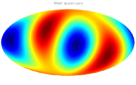
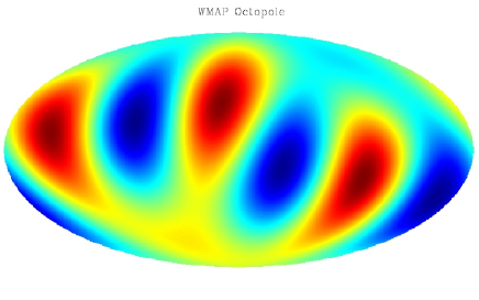
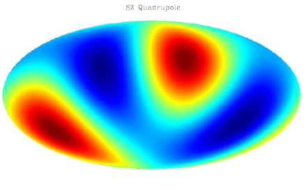
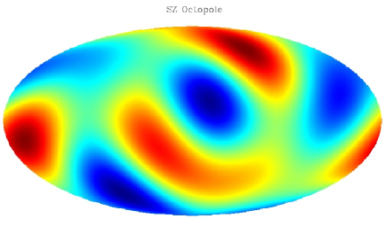
Figure 8: Comparison between the quadrupole (left panels) and octopole (right panels) obtained from the WMAP internal linear combination (ILC) map (upper panels) and from SZ template extracted from the gas simulation (lower panels).

4.4 Detectability of the local SZ signal with the Planck satellite

We investigate now whether the local SZ effect can be observed using the upcoming Planck satellite. The very low noise level and the huge frequency range of the Planck experiment could make it capable of seeing this effect at large scales. Note that the CMB itself is the most important contamination when trying to look for the SZ effect at large scales (Hansen et al., 2005). As the CMB has the same temperature at all frequencies, using a map produced by computing the difference between two frequency bands could be a promising way of detecting the SZ effect (this strategy was attempted for the WMAP data in Hansen et al., 2005). This makes the observation of the SZ effect limited only by the instrumental noise. Unfortunately galactic foregrounds also have several frequency dependent components, and these need to be eliminated at a very high degree in order not to confuse detections of the SZ signal. Here we will assume that these have been completely removed outside a conservative galactic cut.

In order to estimate the sensitivity to the local SZ effect for the Planck experiment, we simulated Planck data for the 70, 100, 143 and 217 GHz channels, by using the technical specifications given at the Planck home page. In more detail, we apply the following procedure.

• For each simulation, we generate a CMB sky and smooth it by using the beams corresponding to the 4 channels of interest. The smoothing is performed in the harmonic space by using beams with size of 14, 9.5, 7.1 and 5 arcmin for the channels at 70, 100, 143 and 217 Ghz, respectively. As the band width for each frequency channel is expected to be much smaller than the frequency difference between the channels, we approximate the band width to be infinitely narrow

• We generate white, non-uniform noise for each channel and add it to the maps. The Planck experiment is expected to have highly correlated noise which would affect the noise power spectrum at the largest scales. Since here we are only interested in a rough estimate of the sensitivity of the Planck experiment to the SZ effect, we neglect this effect. Consequently our results could be slightly over-optimistic at the largest scales.

• We add the SZ template to each map by using the frequency dependence of the SZ effect.

• We construct three different maps, corresponding to the difference between the maps at 217 and 100 GHz (called map A), between 143 and 100 GHz (map B) and between 143 and 70 GHz (map C).

• We apply the Kp0 galaxy and point source mask used by the WMAP team (and publicly available at the Lambda website) before calculating the power spectrum of the difference maps.

In Fig. 9 we show the results of a set of 300 different simulations (the number of simulations has been chosen to obtain error bars correct within a few percent). The solid line corresponds to the power spectrum of the template outside the Kp0 galactic cut. The three shaded areas refer to the $1\sigma$ spread from simulations of the three difference maps, map A having the smallest spread, and map C the largest one. The huge difference between the different pairs comes from two different factors: first, the bigger the frequency difference, the bigger is the SZ effect in the resulting difference map; second, as the CMB is absent in the difference maps, the limiting factor is the noise level which is highly different in different frequency channels. We notice that assuming white noise and a perfect foreground subtraction outside the Kp0 cut, we can expect the local SZ effect to be detected by the Planck satellite. Even if real error bars might be larger than our simulations show, one will still be able to compare data with the predicted local SZ effect. Finally note that analyzing difference maps is a useful tool for checking that foregrounds and other systematic effects of the experiment are well understood. For this purpose it will be of high importance to know well the expected local SZ effect as it will give an important contribution to the difference maps.

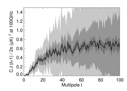
Figure 9: The estimated power spectra of three difference maps from Planck simulations. The solid line shows the power spectrum of the local SZ template. The shaded bands correspond to the $1\sigma$ spread of the estimated power spectra in 300 simulations for the following difference maps: A = 217-100 GHz, B = 143-100 GHz and C = 143-70 GHz. Map A has the lowest spread and map C has the largest one. The Kp0 galactic cut has been used in these simulations. Note that all spectra are normalized to the expected SZ effect at 100 GHz.

5 Conclusions

We used two hydrodynamical cosmological simulations which are designed to represent the observed large-scale structure of the local universe (up to approximately 110 Mpc from the Milky Way) to investigate the imprints of the extended SZ signal caused by local superclusters onto the cosmological full-sky signal. The two simulations, which assume the standard $\Lambda$CDM model, started from the same initial conditions, but included the treatment of a different set of physical processes: the first one assumes adiabatic physics only, while the second one follows also cooling, star formation and supernovae feedback.

We find that the largest and most prominent structures observed in the SZ map constructed from our constrained simulations are caused by local superclusters like Pisces-Perseus or the Centaurus supercluster region. Even Virgo, a relatively poor but nearby cluster, belongs to the most prominent and extended features of the map. Comparing the power spectra of the thermal SZ signal with the one derived from the Hubble volume simulation (Schaefer et al., 2004), we find that for $\ell<100$ these structures lead to an amplitude which is at least twice as high (one order of magnitude for $\ell<20$). When comparing the derived power spectra for the kinetic SZ this factor is even higher.

However, the overall amplitude of the effect is far too small (3-4 orders of magnitude) to have any significant influence on the lowest multipoles of the CMB. There have been some claims that the anomalously low CMB quadrupole and octopole observed by the WMAP satellite could be explained by the imprints of local superclusters. We have shown that the amplitude of the SZ low multipoles must be considerably much higher in order to produce such an effect as well as to have an influence on the observed quadrupole and octopole. Moreover, the directions on the sky of the quadrupole and octopole inferred from our simulations do not coincide with the observed direction in the WMAP maps.

Both for our gas simulation as well as for the Hubble volume simulation, radiative cooling processes and feedback by star formation have been neglected, which could change the absolute amplitude of the inferred SZ signal of galaxy clusters. However, using a simulation which includes all these effects (the csf simulation), we even find a slight decrease of the SZ signal, similar to the findings obtained by using isolated cluster simulations. This will make it even more unlikely to explain the abnormal lower multipoles observed in the WMAP data with the SZ signal of the local universe.

Nevertheless, we find that when taking advantage of the huge frequency range and low noise level of the Planck satellite, an estimate of the SZ power spectrum at large scales could be obtained. We have shown this by producing a set of simulated CMB maps with experimental noise at several frequencies. Analyzing the power spectrum of maps obtained by taking the difference of CMB maps at different frequencies, we show that the power spectrum of the SZ effect is limited only by experimental noise and foreground contamination. We have found that the predicted noise level of the Planck satellite is low enough to allow for the detection of the local SZ power spectrum at low multipoles provided that the galaxy can be removed with sufficient accuracy. It is out of the scope of this work to obtain an accurate estimate of the predicted detection level by the Planck satellite, for which correlated noise as well as an accurate study of foreground removal procedures is required.

References

- Abramo & Sodre (2003) Abramo R., Sodre J., 2003, preprint, astro-ph/0312124
- Afshordi et al. (2004) Afshordi N., Loh Y., Strauss M. A., 2004, Phys. Rev. D, 69, 083524
- Bartelmann (2001) Bartelmann M., 2001, A&A, 370, 754
- Battistelli et al. (2003) Battistelli E. S., De Petris M., Lamagna L., Luzzi G., et al., 2003, ApJ, 598, L75
- Bennett et al. (2003) Bennett C., Bay M., Halpern M., Hinshaw G., et al., 2003, ApJ, 583, 1
- Colberg et al. (2000) Colberg J. M., White S. D. M., Yoshida N., MacFarland T. J., et al., 2000, MNRAS, 319, 209
- Cooray et al. (2004) Cooray A., Baumann D., Sigurdson K., 2004, preprint, astro-ph/0410006
- da Silva et al. (2004) da Silva A. C., Kay S. T., Liddle A. R., Thomas P. A., 2004, MNRAS, 348, 1401
- de Oliveira-Costa et al. (2004) de Oliveira-Costa A., Tegmark M., Zaldarriaga M., Hamilton A., 2004, Phys. Rev. D, 69, 063516
- Diego et al. (2003) Diego J. M., Silk J., Sliwa W., 2003, New Astronomy Review, 47, 855
- Dolag et al. (2005) Dolag K., Grasso D., Springel V., Tkachev I., 2005, JCAP, 1, 9
- Efstathiou (2004) Efstathiou G., 2004, MNRAS, 348, 885
- Efstathiou (2004) Efstathiou G., 2004, MNRAS, 348, 885
- Fixsen (2003) Fixsen D. J., 2003, ApJL, 594, L67
- Fosalba & Gaztañaga (2004) Fosalba P., Gaztañaga E., 2004, MNRAS, 350, L37
- Gaztañaga et al. (2003) Gaztañaga E., Wagg J., Multamäki T., Montaña A., Hughes D. H., 2003, MNRAS, 346, 47
- Górski et al. (1998) Górski K. M., Hivon E., Wandelt B. D., 1998, ‘Analysis Issues for Large CMB Data Sets’, 1998, eds A. J. Banday,R. K. Sheth and L. Da Costa, ESO, Printpartners Ipskamp, NL, pp.37-42 (astro-ph/9812350); Healpix HOMEPAGE: http://www.eso.org/science/healpix/
- Hansen et al. (2005) Hansen F. K., Branchini E., Mazzotta P., Cabella P., Dolag K., 2005, MNRAS, submitted, astro-ph/0502227
- Hernández-Monteagudo et al. (2004) Hernández-Monteagudo C., Genova-Santos R., Atrio-Barandela F., 2004, ApJL, 613, L89
- Hernandez-Monteagudo et al. (2004) Hernandez-Monteagudo C., Genova-Santos R., Atrio-Barandela F., 2004, preprint, astro-ph/0406428
- Hirata et al. (2004) Hirata C. M., Padmanabhan N., Seljak U., Schlegel D., Brinkmann J., 2004, Phys. Rev. D, 70, 103501
- Hoffman & Ribak (1991) Hoffman Y., Ribak E., 1991, ApJ, 380, L5
- Huffenberger et al. (2004) Huffenberger K. M., Seljak U., Makarov A., 2004, Phys. Rev. D, 70, 063002
- Ikebe et al. (2002) Ikebe Y., Reiprich T. H., Böhringer H., Tanaka Y., Kitayama T., 2002, A&A, 383, 773
- Jenkins et al. (2001) Jenkins A., Frenk C. S., White S. D. M., Colberg J. M., Cole S., Evrard A. E., Couchman H. M. P., Yoshida N., 2001, MNRAS, 321, 372
- Kolatt et al. (1996) Kolatt T., Dekel A., Ganon G., Willick J. A., 1996, ApJ, 458, 419
- Mathis et al. (2002) Mathis H., Lemson G., Springel V., Kauffmann G., White S. D. M., Eldar A., Dekel A., 2002, MNRAS, 333, 739
- Mazzotta et al. (2004) Mazzotta P., Rasia E., Moscardini L., Tormen G., 2004, MNRAS, 354, 10
- Mohr et al. (1999) Mohr J. J., Mathiesen B., Evrard A. E., 1999, ApJ, 517, 627
- Monaghan & Lattanzio (1985) Monaghan J. J., Lattanzio J. C., 1985, A&A, 149, 135
- Motl et al. (2005) Motl P. M., Hallman E. J., Burns J. O., Norman M. L., 2005, ApJ, 623, L63
- Myers et al. (2004) Myers A. D., Shanks T., Outram P. J., Frith W. J., Wolfendale A. W., 2004, MNRAS, 347, L67
- Rasia et al. (2005) Rasia E., Mazzotta P., Borgani S., Moscardini L., Dolag K., Tormen G., Diaferio A., Murante G., 2005, ApJ, 618, L1
- Salpeter (1955) Salpeter E. E., 1955, ApJ, 121, 161
- Sanderson et al. (2003) Sanderson A. J. R., Ponman T. J., Finoguenov A., Lloyd-Davies E. J., Markevitch M., 2003, MNRAS, 340, 989
- Schaefer et al. (2004) Schaefer B. M., Pfrommer C., Bartelmann M., Springel V., Hernquist L., 2004, preprint, astro-ph/0407089
- Spergel et al. (2003) Spergel D. N., Verde L., Peiris H. V., Komatsu E., et al., 2003, ApJS, 148, 175
- Springel (2005) Springel V., 2005, preprint, astro-ph/0505010
- Springel & Hernquist (2002) Springel V., Hernquist L., 2002, MNRAS, 333, 649
- Springel & Hernquist (2003) Springel V., Hernquist L., 2003, MNRAS, 339, 289
- Springel et al. (2001) Springel V., Yoshida N., White S., 2001, New Astronomy, 6, 79
- Sunyaev & Zeldovich (1972) Sunyaev R. A., Zeldovich Y. B., 1972, Comments on Astrophysics and Space Physics, 4, 173
- Tegmark et al. (2003) Tegmark M., de Oliveira-Costa A., Hamilton A., 2003, Phys. Rev. D, 68, 123523
- Tornatore et al. (2004) Tornatore L., Borgani S., Matteucci F., Recchi S., Tozzi P., 2004, MNRAS, 349, L19
- Tornatore et al. (2003) Tornatore L., Borgani S., Springel V., Matteucci F., Menci N., Murante G., 2003, MNRAS, 342, 1025
- Vikhlinin (2005) Vikhlinin A., 2005, preprint, astro-ph/0504098
- White et al. (2002) White M., Hernquist L., Springel V., 2002, ApJ, 579, 16