Neutrino emission rates in highly magnetized neutron stars revisited

Magnetars are a subclass of neutron stars whose intense soft-gamma-ray bursts and quiescent X-ray emission are believed to be powered by the decay of a strong internal magnetic field. We reanalyze neutrino emission in such stars in the plausibly relevant regime in which the Landau band spacing $\Delta E$ of both protons and electrons is much larger than $kT$ (where $k$ is the Boltzmann constant and $T$ is the temperature), but still much smaller than the Fermi energies. Focusing on the direct Urca process, we find that the emissivity oscillates as a function of density or magnetic field, peaking when the Fermi level of the protons or electrons lies about $\sim 3kT$ above the bottom of any of their Landau bands. The oscillation amplitude is comparable to the average emissivity when $\Delta E$ is roughly the geometric mean of $kT$ and the Fermi energy (excluding mass), i. e., at fields much weaker than required to confine all particles to the lowest Landau band. Since the density and magnetic field strength vary continuously inside the neutron star, there will be alternating surfaces of high and low emissivity. Globally, these oscillations tend to average out, making it unclear whether there will be any observable effects.

1 Introduction

In recent years, evidence has been accumulating that soft gamma-ray repeaters and anomalous X-ray pulsars are magnetars, strongly magnetized neutron stars powered by the decay of their magnetic field (see Woods & Thompson 2004 for a recent review). The simplest estimate of their magnetic field strength relies on the magnetic dipole braking model usually applied to radio pulsars, which for these objects yields a very strong dipole field, $\sim 10^{14-15}$ G (Kouveliotou et al. 1998; Hurley et al. 1999). Contrary to the case of pulsars, their time-averaged luminosity (in the form of quiescent X-rays and soft gamma-ray bursts) by far exceeds their rotational energy loss, demanding another source of energy, which might be the decay of their internal magnetic field (Duncan & Thompson 1992; Paczyński 1992; Thompson & Duncan 1995, 1996), if this is substantially stronger than the external dipole field.

The observable properties of these objects depend, among other things, on their field strength and their temperature, whose evolution is coupled through the energy dissipated by the field decay and through the thermal modulation of the decay rates (Thompson & Duncan 1996). The most effective cooling mechanism for hot neutron stars is neutrino emission (see, e.g., Yakovlev & Pethick 2004), which also may to some extent control the magnetic field decay (Pethick 1992; Goldreich & Reisenegger 1992). Particularly effective, if allowed, are the direct Urca processes, $n\rightarrow p+e^{-}+\overline{\nu}_{e}$ and $p+e^{-}\rightarrow n+\nu_{e}$, involving neutrons ($n$), protons ($p$), electrons ($e^{-}$), electron neutrinos ($\nu_{e}$), and electron antineutrinos ($\overline{\nu}_{e}$). However, the matter inside a neutron star is highly degenerate. In the absence of an extremely strong magnetic field (far stronger than those discussed above; see Baiko & Yakovlev 1999), Pauli blocking, together with energy and momentum conservation, requires the triangle inequalities

$$|p_{Fp}-p_{Fe}|\leq p_{Fn}\leq p_{Fp}+p_{Fe}$$ (1)

to be at least approximately satisfied for the direct Urca processes to be possible ($p_{Fi}$ is the Fermi momentum of particle $i$, calculated in the non-magnetic approximation). Still, large uncertainties in the composition and equation of state of matter inside neutron stars cores prevent us from deciding whether this condition is fulfilled (e. g., Yakovlev & Pethick 2004). In this paper, we assume that it is, and study the effects of a magnetar-strength field on this simplest neutrino emission process by accounting explicitly for the Landau-band structure of the proton and electron energy levels. We focus on the direct neutron $\beta$ decay ($n\rightarrow p+e^{-}+\overline{\nu}_{e}$) in chemical equilibrium. Other reactions should be affected in a qualitatively similar way, including modified Urca processes in chemical equilibrium or any reactions away from equilibrium, responsible for bulk viscosity (e. g., Finzi 1965; Haensel 1992; Reisenegger 1995).

The magnetic field can make the emissivity change by two effects (Baiko $\&$ Yakovlev 1999). The first relates to the non-trivial spatial form of the wave functions of the charged particles. The second is an increased contribution to the emissivity from the highest Landau band occupied by electrons and/or protons. If the density or the magnetic field are changed, the emissivity oscillates (with an amplitude controlled by the temperature) as new Landau bands become populated or depopulated. The purpose of this work is to perform a detailed study of the second of these effects, quantifying its importance as a function of the different physical parameters involved.

In order to justify the assumptions made in our calculations and to specify the situations in which this work applies, in § 2 we characterize the physical conditions we assume inside the star. In § 3 we describe the calculations performed and the results obtained. A general discussion of the relevance of the results is given in § 4, whereas § 5 lists our main conclusions.

2 Physical Conditions

It is known that a magnetic field $B$ modifies the energy eigenstates and eigenvalues of electrons, protons and neutrons, whose masses we denote as $m_{e}$, $m_{p}$, and $m_{n}$, respectively. The energies of free electrons and protons are given by

$$E_{e}=\sqrt{m^{2}_{e}c^{4}+p^{2}_{ez}c^{2}+2Be\hbar cn}\quad\textrm{ and }\quad E_{p}=\sqrt{m^{2}_{p}c^{4}+p^{2}_{pz}c^{2}+2Be\hbar cm},$$ (2)

where $c$ is the speed of light, $e$ is the charge of the proton, $\hbar$ is the (reduced) Planck constant, and

$$m=l+\frac{1}{2}-\frac{\sigma_{p}}{4}g_{p},\quad{\rm where}\quad l=0,1,2,\ldots\quad{\rm and}\quad\sigma_{p}=\pm 1.$$ (3)

The integer $n$ and non-integer $m$ label the Landau bands of electrons and protons, respectively, $\sigma_{p}$ is the doubled proton spin component along the direction of the magnetic field, $g_{p}=2.79$ is the gyromagnetic ratio of the proton, and $p_{iz}$ is the component of the linear momentum of the particle $i$ along the magnetic field direction.

We note that, within each Landau band, the energy increases continuously with the absolute value of the longitudinal momentum component, $|p_{iz}|$, starting from a bottom value corresponding to $p_{iz}=0$, which, for simplicity, we will refer to as the Landau level corresponding to this band. As the density increases in degenerate matter at a given magnetic field strength, new Landau bands get populated as the Fermi energy, $E_{Fi}$, increases, leading to oscillating thermodynamic functions (see, e. g., Dib & Espinosa 2001). Here, our main focus will be on similar oscillations in the neutrino emissivity.

We ignore the effect of inter-particle forces on the energy levels of the charged particles. This is a good approximation for the electrons, which do not interact strongly. However, strong interactions do modify the eigenvalues of energy of the protons, whose Landau levels tend to broaden. We discuss below the importance of this broadening for the contribution to the emissivity from the highest Landau band occupied by protons.

If we neglect strong interactions for the neutrons as well, the second triangle inequality in eq. (1) would never be satisfied, and direct Urca reactions would be forbidden (e.g., Shapiro & Teukolsky 1983). Thus, for consistency, we allow for an arbitrary dispersion relation $E_{n}(p_{n})$ for the neutrons, which takes their strong interactions into account and could in principle allow direct Urca processes to take place, even in the absence of a magnetic field. This relation defines an effective mass for the neutron, $m_{n}^{*}\equiv p_{Fn}/[dE_{n}/dp_{n}]_{p_{Fn}}$, which is generally somewhat smaller than the “bare” mass, $m_{n}$. Here and throughout this paper, we ignore the relatively small dependence of the neutron dispersion relation on the spin projection along the magnetic field.

In order to specify the physical conditions to be considered, we define the dimensionless quantities

$$n_{M}\equiv\frac{E^{2}_{Fe}-m_{e}^{2}c^{4}}{2Be\hbar c}\textrm{ , }m_{M}\equiv\frac{E^{2}_{Fp}-m_{p}^{2}c^{4}}{2Be\hbar c},\textrm{ and }r\equiv\frac{p_{Fn}^{2}c}{2Be\hbar},$$ (4)

where the integer part of $n_{M}$ corresponds to the highest Landau band populated by electrons in the zero-temperature limit. The same role is played for the protons by the largest value of $m\leq m_{M}$ compatible with eq. (3). We note that each of these can quantitatively be written as $\approx 150\rho_{37}^{2/3}/B_{16}$, where the number density of the relevant particles is $\rho=\rho_{37}\times 10^{37}{\rm cm}^{-3}$ and the magnetic field is $B=B_{16}\times 10^{16}{\rm G}$. It is also useful to identify the energy difference between adjacent Landau levels for the particle $i=e,p$,

$$\Delta E_{i}\sim\frac{Be\hbar c}{E_{i}},$$ (5)

which takes the values $\Delta E_{e}\approx 0.5B_{16}/\rho_{37}^{1/3}$ MeV for the (highly relativistic) electrons and $\Delta E_{p}\approx 0.06B_{16}$ MeV for the (approximately non-relativistic) protons. We assume that the electrons, protons, and neutrons are in chemical equilibrium and consider, for the calculation of the transition probabilities of the direct $\beta$ decay, that the protons and neutrons are non-relativistic particles.

Most importantly, we will see below that, in order for the Landau band structure to be noticeable, the magnetic field must be at least strong enough to make $\Delta E_{i}\sim 10kT$, where $k$ is the Boltzmann constant and $T$ is the temperature. However, magnetic fields expected to exist in magnetars are still so weak as to make $r$, $n_{M}$, and $m_{M}\gg 1$, which means that the electrons and protons populate many Landau bands. Writing $T=T_{8}\times 10^{8}{\rm K}$, these conditions constrain the magnetic field to the range

$$T_{8}\ll B_{16}\ll 10^{2}\rho_{37}^{2/3}.$$ (6)

While the upper bound is easily satisfied by all observational evidence, the lower bound is not obviously true in any known case. Indeed, the lower bound (here given for protons, although a less stringent condition for electrons also exists: $0.1T_{8}\rho_{37}^{1/3}\ll B_{16}$) might not be satisfied even for magnetars, despite their very strong $B$ fields, because the dissipation of their huge magnetic energy tends to keep their interiors fairly hot. If that is the case, the magnetic field effects we are studying here are negligible. Nevertheless, given the possibility that this regime may be applicable, we proceed to explore its consequences.

3 Emission rate calculations

We calculate the neutrino emissivity due to the direct $\beta$ decay using the Weinberg-Salam-Glashow theory of weak interactions. We confirm Baiko & Yakovlev’s (1999) eqs. (5) and (8) for the power radiated per unit volume,

$$Q_{\bar{\nu}}=\frac{2Be}{(2\pi)^{7}\hbar^{9}c}\sum_{n,l,\sigma_{p},\sigma_{n}}\int d^{3}p_{n}d^{3}p_{\bar{\nu}}dp_{ez}dp_{pz}E_{\bar{\nu}}f_{n}(1-f_{p})(1-f_{e})\delta(\Delta E)\delta(\Delta p_{z})M,$$ (7)

where

$$M=G_{F}^{2}\left\{2g_{A}^{2}\left[\delta_{\sigma_{p},1}\delta_{\sigma_{n},-1}F_{n,l}^{2}(u)+\delta_{\sigma_{p},-1}\delta_{\sigma_{n},1}F_{n-1,l}^{2}(u)\right]+{1\over 2}\delta_{\sigma_{p},\sigma_{n}}\left[(1+g_{A}\sigma_{p})^{2}F_{n-1,l}^{2}(u)+(1-g_{A}\sigma_{p})^{2}F_{n,l}^{2}(u)\right]\right\},$$ (8)

$u=c\{p_{n}^{2}-(p_{ez}+p_{pz})^{2}\}/(2Be\hbar)$, $\Delta E=E_{n}-E_{p}-E_{e}-E_{\bar{\nu}}$, $\Delta p_{z}=p_{nz}-p_{ez}-p_{pz}$, and $f_{i}$ is the Fermi-Dirac factor corresponding to the particle $i$. The Fermi weak coupling constant is $G_{F}=1.399\times 10^{-49}$ $\textrm{erg}\textrm{ }\textrm{cm}^{3}$, and $g_{A}=1.261$ is the nucleon axial-vector coupling. The Laguerre functions $F_{n,l}(u)$ are defined in the Appendix (and are taken to vanish when one of their indices is negative). The physical conditions discussed in §2 have already been used to neglect the antineutrino momentum, $p_{\bar{\nu}}\sim kT/c\ll p_{Fn}$, both in the definition of the variable $u$ and in the momentum-conserving delta function. In principle, it contributes to the “thermal smoothing” discussed below, but to a lesser degree than the antineutrino energy, which we keep in our calculation.

The integrals over directions of motion for antineutrinos and neutrons are easily done (the latter eliminates the momentum-conserving delta function), and the energies of antineutrinos, electrons, and protons can be used as new integration variables, yielding

$$Q_{\bar{\nu}}=\frac{4Be}{(2\pi)^{5}\hbar^{9}c^{6}}\sum_{n,l,\sigma_{p},\sigma_{n},\gamma}\int_{0}^{\infty}dE_{\bar{\nu}}\int_{0}^{\infty}dp_{n}\int_{a_{e}}^{\infty}dE_{e}\int_{a_{p}}^{\infty}dE_{p}\frac{p_{n}E_{\bar{\nu}}^{3}E_{e}E_{p}f_{n}(1-f_{p})(1-f_{e})\delta(\Delta E)\Theta(u)M}{\sqrt{E_{p}^{2}-m_{p}^{2}c^{4}-2Be\hbar cm}\sqrt{E_{e}^{2}-m_{e}^{2}c^{4}-2Be\hbar cn}},$$ (9)

where $a_{e}=\sqrt{m_{e}^{2}c^{4}+2Be\hbar cn}$ and $a_{p}=\sqrt{m_{p}^{2}c^{4}+2Be\hbar cm}$, and $\Theta(u)$ is the usual Heaviside step function. The values of the new variable $\gamma=\pm 1$ label the cases in which $p_{ez}$ and $p_{pz}$ have equal and opposite signs, respectively, affecting the value of $u={\left[p_{n}^{2}c^{2}-\left(\sqrt{E_{e}^{2}-m^{2}_{e}c^{4}-2Be\hbar cn}+\gamma\sqrt{E_{p}^{2}-m^{2}_{p}c^{4}-2Be\hbar cm}\right)^{2}\right]/(2Be\hbar c)}.$

If the particles are in chemical equilibrium, the Fermi-Dirac factors suppress those reactions in which the difference between the energy of the reacting particles and their corresponding Fermi energies is much larger than $kT$. This fact allows to also change the integration variable for the neutrons, as $p_{n}dp_{n}=m_{n}^{*}dE_{n}$, and to set $E_{i}=E_{Fi}$ in those terms where a variation of the energy of order $kT$ makes very little difference.

For instance, in the Appendix it is shown that there is a range in which $F_{m,n}(u)$ behaves as an oscillating function and that, outside this range, this function decays exponentially. The average oscillation period is $\approx 4\sqrt{{\max\{n,m\}}/{\min\{n,m\}}}>1,$ much larger than the variation in $u$ due to an energy change $\sim kT$, $\delta u\sim kT/\Delta E_{p}\ll 1$. Therefore, in the variable $u$, we can safely set $E_{i}=E_{Fi}$, and obtain $u=r-\left(\sqrt{n_{M}-n}+\gamma\sqrt{m_{M}-m}\right)^{2}$, where $r$, $n_{M}$ and $m_{M}$ were defined in (4).

With the factors $\sqrt{E_{e}^{2}-m_{e}^{2}-2Be\hbar cn}$ and $\sqrt{E_{p}^{2}-m_{p}^{2}-2Be\hbar cm}$ in the denominator of eq. (9), we cannot always do the same. Since they could eventually vanish for the highest Landau band of each particle, a variation of the energy of order $kT$ could become crucial in the emission rate we want to calculate.

Let us first consider a situation in which this is not an issue, i.e., none of the Landau levels of the particles is too close to the respective Fermi energy,

$$\left|E_{Fe}-\sqrt{m_{e}^{2}c^{4}+2Be\hbar cn}\right|\gg kT\textrm{ }\textrm{ and }\textrm{ }\left|E_{Fp}-\sqrt{m_{p}^{2}c^{4}+2Be\hbar cm}\right|\gg kT$$ (10)

for all $n$ and $m$. In this case, we can set $E_{e}=E_{Fe}$ and $E_{p}=E_{Fp}$, obtaining

$$\overline{Q}_{\bar{\nu}}=\frac{457\pi m_{n}^{*}m_{p}E_{Fe}(kT)^{6}}{80640\hbar^{10}c^{5}}\sum_{\gamma=\pm 1}\sum_{\sigma_{n}=\pm 1}\sum_{\sigma_{p}=\pm 1}\sum_{n=0}^{\lfloor n_{M}\rfloor}\sum_{l=0}^{l_{max}}\frac{\Theta(u)M}{\sqrt{n_{M}-n}\sqrt{m_{M}-m}}\textrm{ , }$$ (11)

where the symbol $\lfloor\textrm{ }\rfloor$ denotes the integer part, and $l_{max}={\lfloor m_{M}-{1\over 2}+{\sigma_{p}g_{p}\over 4}\rfloor}$.

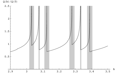
Figure 1: Magnetic-field dependent emissivity (normalized by the zero-field value) at low temperatures, as approximated by eq. (11), for $r=100/b$ and $n_{M}=m_{M}=40/b$, corresponding to constant particle number densities, $\rho_{e}=\rho_{p}=0.25\rho_{n}$, and a magnetic field $B=6.8\times 10^{16}b\left(\rho_{n}/10^{38}{\rm cm}^{-3}\right)^{2/3}$ G. The shading identifies those regions where thermal effects at temperatures $T\sim 10^{9}$ K would strongly affect the emissivity.

In Fig. 1, we show a numerical calculation of this double sum for fixed densities of all particles, and a variable magnetic field. The true emissivity will deviate from this result (and the formal divergences will be smoothed, as discussed below) in those regions where the condition (10) does not hold. As an example, the shading in our graph identifies these regions for a temperature $\sim 10^{9}$ K. Still, it is instructive to note that the peaks come in “triplets”, in which the central (and strongest) peak corresponds to a spin-degenerate electron Landau level coinciding with its Fermi energy, whereas the two flanking peaks correspond to similar coincidences for the (non-degenerate) proton Landau levels, for opposite spins. Their symmetric spacing arises automatically when the proton and electron densities are equal, as is the case in charge neutrality, when protons and electrons are the only charge carriers, but does not necessarily occur when other charge carriers (muons, mesons, or hyperons) are also present in the system.

Much less conspicuous are the discontinuities caused by the step function $\Theta(u)$ that ensures momentum conservation along the magnetic field. Since, as $u\to 0$, the Laguerre functions behave as $F_{n,l}\sim u^{|n-l|}$ (see eq. 18), a true discontinuity in the emissivity (rather than in one of its derivatives) arises only for terms with $n=l$ (in which the spatial wave functions of protons and electrons coincide). Some of these are barely visible in Fig. 1, at $b\approx$ 2.94, 3.06, 3.25, and 3.40. These will also tend to be washed out by thermal effects, so we doubt that they could have any astrophysical significance.

An average value for $\overline{Q}_{\bar{\nu}}$ can be obtained by making some approximations for the behavior of the Laguerre functions $F_{n,l}$ when $n$, $l$, and $|n-l|$ are all large. We take the average expression for the functions $F_{m,n}^{2}(u)$ in the interval where they oscillate (eq. [30]), and $F_{m,n}^{2}(u)=0$ where they undergo an exponential decay (see Appendix). Then, approximating the sums over $n$ and $l$ as integrals and neglecting the spin dependence of the particles’ energies, we find

$$\overline{Q}_{\bar{\nu}}=G_{F}^{2}(1+3g_{A}^{2})\frac{457\pi m_{n}^{*}m_{p}E_{Fe}(kT)^{6}}{20160\textrm{ }\hbar^{10}c^{5}},$$ (12)

which agrees with the unmagnetized case (Lattimer et al. 1991).

The approximations leading up to eq. (11) are exact in the limit of vanishing temperature, but clearly break down at finite temperature when one of the Landau levels approaches the Fermi energy of the respective particle species, so the condition (10) is not satisfied for this level. The contribution of the latter to the total emissivity becomes very large (formally divergent, in the approximation considered above) and is no longer well-approximated by the corresponding term in the expression (11). In order to determine the importance of this effect, we must compute the contribution of this Landau band independently and, then, compare it to $\overline{Q}_{\bar{\nu}}$ as given by eq. (12), which still gives a reasonable approximation to the contribution of all the other bands.

We focus on the case in which one of the Landau levels of the electrons, labelled as $\hat{n}$ (either $\hat{n}=\lfloor n_{M}\rfloor$ or $\hat{n}=\lfloor n_{M}\rfloor+1$), is close to their Fermi energy, i. e., $|E_{Fe}-\sqrt{m_{e}^{2}c^{4}+2Be\hbar c\hat{n}}|\sim kT$, but the same does not happen for the protons. The contribution of the electron Landau band $\hat{n}$ to the emissivity, obtained from the appropriate term in eq. (9), summed over all proton Landau bands, and using the same approximations for $F_{\hat{n},l}^{2}(u)$ as in equation (12), is

$$\hat{Q}_{\bar{\nu}}=G_{F}^{2}(1+g_{A}^{2})\frac{Be\hbar cm_{n}^{*}m_{p}E_{Fe}}{2^{3}\pi^{5}\hbar^{10}c^{5}}(kT)^{5}\sqrt{\frac{2kT}{E_{Fe}(E_{Fe}^{2}-m_{e}^{2}c^{4})}}I(x),$$ (13)

where $x\equiv(E_{Fe}-\sqrt{m_{e}^{2}c^{4}+2Be\hbar c\hat{n}})/(kT)$ and

$$I(x)\equiv\int_{0}^{\infty}\int_{0}^{\infty}\frac{t^{3}(t+u-x)dudt}{u^{\frac{1}{2}}(e^{x-u}+1)(e^{t+u-x}-1)}.$$ (14)

Figure 2: The function $I(x)$, evaluated numerically from eq. (14).

In Figure 2, we can see that this function has a peak at $x=3.08$, where its value is $53.8$, decreasing as $I(x)\approx 457{\pi}^{6}/(5040\sqrt{x})$ for $x\gg 3$, and exponentially for $x<0$. The smooth shape of this function (left-right reversed, since $x$ is a decreasing function of $B$) is the true shape of the divergent peaks of Fig. 1 at finite temperature.

4 Discussion

We compare the emissivity contribution of the highest significantly populated electron Landau band to the unmagnetized emissivity (which approximates the contribution from all the other Landau bands) by computing the ratio

$$\frac{\hat{Q}_{\bar{\nu}}}{\overline{Q}_{\bar{\nu}}}\approx\frac{I(x)}{123}\frac{Be\hbar c}{\sqrt{kTE_{Fe}(E_{Fe}^{2}-m_{e}^{2}c^{4})}}\approx{I(x)\over 123}{\Delta E_{e}\over\sqrt{kTE_{Fe}}}.$$ (15)

As the density is increased or the magnetic field is decreased, the emissivity oscillates as new Landau bands start populating. Assuming, for definiteness, that the control parameter is $E_{Fe}$, and ignoring variations of $E_{Fp}$ for now, these variations are roughly periodic with a period $\Delta E_{e}$, on which asymmetric peaks occur (sharply rising as the Landau level starts populating, slowly decreasing afterwards), with a total width at half maximum $\sim 10kT$. If $\Delta E_{e}\gg 10kT$, the fractional amplitude of the oscillations is $\sim 0.4\Delta E_{e}/\sqrt{kTE_{Fe}}$, becoming comparable to the total emissivity when the level spacing is the geometric mean of $kT$ and the Fermi energy or, equivalently, $B\sim 10^{17}\sqrt{T_{8}\rho_{37}}{\rm G}$, probably higher than is reached in magnetars.

In the case of the protons, the situation is different. Since they interact strongly, their dispersion relation is not exactly the one shown in eq. (2). Strong interactions, mainly with the neutrons, broaden the Landau levels of the protons. If this broadening is of order or larger than the spacing between the levels, the effect of emissivity oscillations given by the filling of their consecutive Landau bands tends to disappear. On the other hand, even if the protons did not interact strongly, the importance of the emissivity contribution of their highest populated Landau band would be subdominant in comparison to the one of the electrons. This can be seen directly from eq. (15), taking into account two facts. First, proton Landau bands are not spin degenerate, so the expression for the ratio $\hat{Q}_{\bar{\nu}}/\overline{Q}_{\bar{\nu}}$ is reduced by a factor 1/2. Second, their larger mass implies (at the same density) a smaller Landau-level spacing, yielding a more stringent condition to see substantial oscillations, and a smaller amplitude for these. It also implies that the last expression in eq. (15) would not be directly applicable, but would have to be replaced by a similar one, in which the mass term $m_{p}c^{2}$ is subtracted from the Fermi energy.

In a neutron star in diffusive equilibrium, the redshifted total chemical potential (including electrostatic potential energy) for each particle species is uniform throughout the region where the respective species is present. Since the redshift factor is a smooth function of position, so will be the local (or “intrinsic”) chemical potentials, i. e., the Fermi energies considered in this work except at phase boundaries, where the electrostatic potentials can be discontinuous. We stress that this does not imply that the particle densities are smooth functions of position, but will rather have oscillations superimposed on the smooth increase with increasing Fermi energy, as illustrated, e.g., in Fig. 2 of Dib & Espinosa (2001).

More directly to the point of this paper, even if the magnetic field is uniform, the smooth spatial variation of the Fermi energies will make the emissivity an oscillating function of position. Shells of larger and smaller emissivity will alternate within the star. If the magnetic field strength is truly uniform, these shells will be spherical, constant-density surfaces, otherwise they can be arbitrarily convolved.

The observational relevance of this is not clear. As said above, in each “period” $\Delta E_{e}$, the emissivity peak has a width $\sim 10kT$ and a fractional height $\sim 0.4\Delta E_{e}/\sqrt{kTE_{Fe}}$, so its fractional contribution to the total emissivity over the corresponding period is $\sim(10kT/\Delta E_{e})(0.4\Delta E_{e}/\sqrt{kTE_{Fe}})=4\sqrt{kT/E_{Fe}}$. The degeneracy condition $kT\ll E_{Fe}$ is amply satisfied in all neutron stars more than a few seconds old, so the contribution of the peaks to the total emissivity is very small.

5 Conclusions

We have shown that, in the regime in which the Landau level separation is intermediate between $kT$ and the Fermi energies (excluding $mc^{2}$), the direct Urca emissivity is strongly enhanced when the Fermi energy of electrons or protons lies $\sim 3kT$ above the bottom of any of the Landau bands. Thus, it will oscillate as a function of density or field strength. The oscillation amplitude becomes comparable to the total emissivity when the level separation is near the geometric mean of the other two energy scales. The required conditions may be present in magnetars, but this is not guaranteed. Even if it were the case, the large number of emissivity oscillations expected inside a given star could average out to give nearly the same global cooling rate as in an unmagnetized star, so their observational consequences are far from obvious.

Appendix A Some properties of the Laguerre functions

For easy reference, in this Appendix we summarize some useful properties of the Laguerre functions, $F_{m,n}(u)$. These results were obtained by Kaminker $\&$ Yakovlev (1980, 1981).

The Laguerre functions with indices $m,n=0,1,2,...$ are defined as

$$F_{m,n}(u)=\left\{\begin{array}[]{cc}\sqrt{n!/m!}(-1)^{a}e^{-\frac{u}{2}}u^{\frac{a}{2}}L_{n}^{a}(u),&{\rm for}\quad m\geq n\\ (-1)^{a}F_{n,m}(u)&{\rm otherwise}\end{array}\right.$$ (18)

where $a=m-n$ and $L_{n}^{a}(u)$ correspond to the Laguerre polynomials,

$$L_{n}^{a}(u)=\sum_{k=0}^{n}\frac{\Gamma(n+a+1)}{\Gamma(k+a+1)}\frac{(-u)^{k}}{k!(n-k)!}.$$ (19)

Defining $f(u)=\frac{1}{4u^{2}}(u-u_{-})(u-u_{+})$, where $u_{\pm}=(m+n+1)\pm\sqrt{4mn+2(m+n)+2}$, approximate expressions for $F_{m,n}(u)$ for different ranges of $u$ in the limit $n,m,|n-m|\gg 1$, can be given as follows:

• For $u_{-}-u\gg\left(\frac{u_{-}^{2}}{u_{+}-u_{-}}\right)^{\frac{1}{3}}$,

  $$F_{m,n}(u)=(-1)^{\frac{a+|a|}{2}}\left\{4\pi u\sqrt{f(u)}\right\}^{-\frac{1}{2}}e^{u\sqrt{f(u)}-\phi}.$$ (20)

• For $u-u_{+}\gg\left(\frac{u_{+}^{2}}{u_{+}-u_{-}}\right)^{\frac{1}{3}}$,

  $$F_{m,n}(u)=(-1)^{m}\left\{4\pi u\sqrt{f(u)}\right\}^{-\frac{1}{2}}e^{-u\sqrt{f(u)}-\phi},$$ (21)

  where

  $$\phi=\frac{u_{-}+u_{+}}{4}\ln\left(\frac{\left\{\sqrt{|u-u_{+}|}-\sqrt{|u-u_{-}|}\right\}^{2}}{u_{+}-u_{-}}\right)\textrm{ }+\textrm{ }\frac{\sqrt{u_{-}u_{+}}}{2}\ln\left(\frac{\left\{\sqrt{u_{-}|u-u_{+}|}+\sqrt{u_{+}|u-u_{-}|}\right\}^{2}}{u\{u_{+}-u_{-}\}}\right).$$ (22)

• For $|u-u_{-}|\ll u_{-},u_{+}-u_{-}$,

  $$F_{m,n}(u)=(-1)^{\frac{a+|a|}{2}}\left\{\frac{4}{u_{-}(u_{+}-u_{-})}\right\}^{\frac{1}{6}}{\rm Ai}\left(\{u_{-}-u\}\left\{\frac{u_{+}-u_{-}}{4u_{-}^{2}}\right\}^{\frac{1}{3}}\right).$$ (23)

• For $|u-u_{+}|\ll u_{+}-u_{-}$,

  $$F_{m,n}(u)=(-1)^{m}\left\{\frac{4}{u_{+}(u_{+}-u_{-})}\right\}^{\frac{1}{6}}{\rm Ai}\left(\{u-u_{+}\}\left\{\frac{u_{+}-u_{-}}{4u_{+}^{2}}\right\}^{\frac{1}{3}}\right),$$ (24)

  where ${\rm Ai}(x)$ corresponds to the Airy function of the first kind (see, for example, Lebedev 1972).The asymptotic behavior of this function,

  $${{\rm Ai}(x)\approx\left\{\begin{array}[]{cc}\frac{\pi^{-\frac{1}{2}}}{2}x^{-\frac{1}{4}}e^{-\frac{2}{3}x^{\frac{3}{2}}}&x\rightarrow\infty\\ \pi^{-\frac{1}{2}}|x|^{-\frac{1}{4}}\cos(\frac{2}{3}|x|^{\frac{3}{2}}-\frac{\pi}{4})&x\rightarrow-\infty\textrm{,}\end{array}\right.}$$ (27)

  shows us that the Laguerre functions oscillate between $u_{-}$ and $u_{+}$ and decay exponentially outside this range.

• For $u-u_{-}\gg\left(\frac{u_{-}^{2}}{u_{+}-u_{-}}\right)^{\frac{1}{3}}$ and $u_{+}-u\gg\left(\frac{u_{+}^{2}}{u_{+}-u_{-}}\right)^{\frac{1}{3}}$, we have

  $$F_{m,n}=\left\{\pi u\sqrt{-f(u)}\right\}^{-\frac{1}{2}}\cos\left(u\sqrt{-f(u)}-\varphi\right),$$ (28)

  where

  $$\varphi=\frac{u_{-}+u_{+}}{4}\sin^{-1}\left(\frac{u_{-}+u_{+}-2u}{u_{+}-u_{-}}\right)\textrm{ }-\textrm{ }\frac{\sqrt{u_{+}u_{-}}}{2}\sin^{-1}\left(\frac{2u_{-}u_{+}-u\{u_{-}+u_{+}\}}{u\{u_{+}-u_{-}\}}\right)-\frac{\pi}{4}\left(m+n+2a+|a|\right).$$ (29)

  In this work we use the average expression for $F_{m,n}^{2}(u)$ in this range,

  $$\langle F_{m,n}^{2}\rangle=\pi^{-1}\left\{(u-u_{-})(u_{+}-u)\right\}^{-\frac{1}{2}}.$$ (30)

- (1) Baiko, D. A. & Yakovlev, D. G. 1999, A&A, 342, 192
- (2) Dib, C. O., & Espinosa, O. 2001, Nuclear Physics B, 612, 492
- (3) Duncan, R. C. & Thompson, C. 1992, ApJ, 392, L9
- (4) Finzi, A. 1965, Phys. Rev. Lett., 15, 599
- (5) Goldreich, P., & Reisenegger, A. 1992, ApJ, 395, 250
- (6) Haensel, P. 1992, A&A, 262, 131
- (7) Hurley, K., Li, P., Kouveliotou, C., et al. 1999, ApJ, 510, L111
- (8) Kaminker, A. D. & Yakovlev, D. G. 1980, Calculation of elementary processes with relativistic electrons in a quantizing magnetic field, unpublished.
- (9) Kaminker, A. D. & Yakovlev, D. G. 1981, Theoretical and Mathematical Physics 49, 1012.
- (10) Kouveliotou, C., Dieters, S., Strohmayer, T., et al. 1998, Nature, 393, 235
- (11) Lattimer, J. M., Pethick, C. J., Prakash, M. & Haensel, P. 1991, Phys. Rev. Lett., 66, 2701
- (12) Lebedev, N. N. 1972, Special functions & their applications (New York: Dover)
- (13) Paczynski, B. 1992, Acta Astron., 42, 145
- (14) Pethick, C. J. 1992, in The Structure and Evolution of Neutron Stars, eds. D. Pines, R. Tamagaki, & S. Tsuruta (Redwood City: Addison-Wesley), p. 115
- (15) Reisenegger, A. 1995, ApJ, 442, 749
- (16) Thompson, C. & Duncan, R. C. 1995, MNRAS, 275, 255
- (17) Thompson, C. & Duncan, R. C. 1996, ApJ, 473, 322
- (18) Woods, P. M., & Thompson, C. 2004, to appear in Compact Stellar X-ray Sources, eds. W. G. H. Lewin & M. van der Klis (astro-ph/0406133)
- (19) Yakovlev, D. G. & Pethick, C. J. 2004, ARA&A, 42, 169