The enigmatic B[e]-star Henize 2-90: The non-spherical mass loss history from an analysis of forbidden lines

We study the optical spectrum of the exciting B[e] star Hen 2-90 based on new high-resolution observations that cover the innermost 2″of the object whose total extent is more than 3″. Our investigation is splitted in two parts, a qualitative study of the presence of the numerous emission lines and the classification of their line profiles which indicate a circumstellar environment of high complexity, and a quantitative analysis of numerous forbidden lines, e.g. [Oi], [Oii], [Oiii], [Sii], [Siii], [Ariii], [Clii], [Cliii] and [Nii]. We find a correlation between the different ionization states of the elements and the velocities derived from the line profiles: the highly ionized atoms have the highest outflow velocity while the neutral lines have the lowest outflow velocity. The recent HST image of Hen 2-90 (Sahai et al. Sahai02 (2002)) reveals a bipolar, highly ionized region, a neutral disk-like structure and an intermediate region of moderate ionization. This HST image covers about the same innermost regions as our observations. When combining the velocity information with the HST image of Hen 2-90 it seems that a non-spherical stellar wind model is a good option to explain the ionization and spatial distribution of the circumstellar material. Such a wind might expand into the cavity formed during the AGB phase of the star which is still visible as a large nebula, seen e.g. on H$\alpha$ plates. We modelled the forbidden lines under the assumption of a non-spherically symmetric wind that can be split into a polar, a disk forming and an intermediate wind, based on the HST image. We find that in order to fit the observed line luminosities, the mass flux, surface temperature, and terminal wind velocities need to be latitude dependent, which might be explained in terms of a rapidly rotating central star. A rotation speed of 75–80% of the critical velocity has been derived from the terminal velocities, extracted from the observed line wings considering the inclination of the system as suggested from the HST image. The total mass loss rate of the star was determined to be of order $3\times 10^{-5}$ M_⊙yr^-1. Such a wind scenario and the fact that compared to solar abundances C, O, and N seem to be underabundant while S, Ar and Cl have solar abundances, might be explained in terms of a rapidly rotating post-AGB star.

1 Introduction

Hen 2-90 (PN Sa 2-90, PN G305.1+01.4, IRAS 13064-6103) is a very interesting object whose evolutionary stage is unclear. Its distance was estimated to be about $d\,=1.5$ kpc by Costa et al. (Costa (1993)) while Sahai & Nyman (Sahai00 (2000)) adopted $d\,=2.5$ kpc. Its effective temperature was estimated to be $51000$ K (Kaler & Jacoby, Kaler (1991)) and its luminosity was derived to be $\log(L/L_{\sun})\sim 3.0$ (Costa et al., Costa (1993)).

The star was firstly classified as a planetary nebula by Webster (Webster (1966)) and Henize (Henize (1967)). Later, Costa et al. (Costa (1993)) and Maciel (Maciel (1993)) classified it as a planetary nebula with low metal abundance and with a central star of low mass and low luminosity. Lamers et al. (Lamers98 (1998)) included it in the list of objects presenting the B[e] phenomenon, as a compact planetary nebula B[e].

Sahai & Nyman (Sahai00 (2000)), based on HST images, and Guerrero et al. (Guerrero (2001)), using ground based images, have described the presence of a nebula bisected by a disk and with a bipolar jet and knots, spaced uniformly. Guerrero et al. (Guerrero (2001)) noted that the dynamical stability of the jets and knots makes Hen 2-90 a unique object. These characteristics could point to a compact planetary nebula, since many planetary nebulae present a bipolar nebula. This fact implies that the asymmetries in the wind can already take place in the late stages of the AGB phase, where the jets can probably shape the spherical AGB wind in a bipolar scenario (Sahai & Trauger, Sahai98 (1998); Imai et al., Imai (2002); Vinković et al., Vinkovic (2004)). However, the presence of a disk and jets could also be explained assuming that the system is a binary (Sahai & Nyman, Sahai00 (2000)). Guerrero et al. (Guerrero (2001)) also noted, that based on near-IR colors, Hen 2-90 might be a symbiotic system, i.e. a binary composed of a cool giant and a hot component with an accretion disk. Due to these two completely different interpretations (compact planetary nebula or symbiotic object) the real nature of Hen 2-90 stays unclear.

We study this object by means of high-resolution spectroscopy and low resolution spectrophotometry data obtained with the FEROS and B&C spectrographs, respectively, at the 1.52m telescope in ESO (La Silla, Chile). The goals of this study are:

• to describe the spectral features in the optical spectrum, obtained with a resolution higher than any other published observation to date;

• to study the circumstellar material of this star (temperature and density distribution, velocities, ionization structure) using the spectrophotometrically calibrated line profiles.

For the first goal, we will describe the various line profiles and associated Doppler velocities of the different types of lines. For the second one, we will make a complete analysis of all the forbidden emission lines (except of lines of Feii).

The structure of the paper is as follows. In Sect. 2 we give the information about our observations. In Sect. 3 we present a spectral atlas obtained from our optical data, showing the different line profiles identified in the spectra. In Sect. 4 we discuss the nature of the circumstellar material whether it is a shell, nebula or a stellar wind. In Sect. 5 we derive the total mass loss rate of the star from modeling the forbidden emission lines in the scenario of a non-spherically symmetric wind. In Sect. 6 we discuss the validity of our assumptions and discuss the non-spherical wind scenario in terms of a rapidly rotating star. In addition, we discuss the nature of Hen 2-90, as being either a compact planetary nebula or a symbiotic object, based on abundance criteria found from the analysis and on spectral characteristics in our new high-resolution observations. In Sect. 7 we summarize our conclusions.

2 Observations & Reductions

High and low resolution observations were obtained with the Fiber-fed Extended Range Optical Spectrograph (FEROS) and with the Boller & Chivens (B&C) spectrograph, respectively, at the ESO 1.52m telescope in La Silla (Chile). FEROS is a bench-mounted Echelle spectrograph with the fibers located at the Cassegrain focus with a spectral resolution of R = 48 000 corresponding to 2.2 pixels of 15 $\mu$m and with a wavelength coverage from 3600 Å to 9200 Å. The aperture of FEROS through which the fibers are illuminated is 2$\arcsec$.

High resolution observations of Hen 2-90 (higher than the spectra previously described in the literature) were taken on 2000 June 10, with an exposure time of 4800 seconds. These data were used to get a spectral atlas, a detailed description of the line profiles and also to deblend some features present in the low resolution spectra. The S/N ratio in the 5500 Å region is aproximately 20. FEROS has a complete automatic on-line reduction, that was adopted by us. Equivalent widths have been measured using an IRAF task that computes the line area above the adopted continuum.

Low resolution spectra of Hen 2-90 were taken on 2000 June 9, with an exposure time of 900 seconds. The slit width was 2$\arcsec$. The instrumental setup employed made use of grating #23 with 600 l mm^-1, providing a resolution of $\sim 4.6$ Å in the range 3800-8700 Å. The efficiency of the CCD is a function of wavelength. It increases from about 70% at 3500 Å to its maximum value of 90% at about 7000 Å and then decreases again, reaching 75% at 8000 Å. This behaviour results in larger flux uncertainties of about 20% especially in the very low ($<5000$Å) and very high ($>7500$Å) wavelength regions of the spectrum, while in the range in between the flux uncertainties are more of order 10%. In the 5500 Å region, the S/N ratio in the continuum is aproximately 40 for the B&C spectrum (hereafter Cassegrain spectrum). Since there is no completely line free region in the spectrum, the S/N derived is an upper limit. The Cassegrain spectra were reduced using standard IRAF tasks, such as bias subtraction, flat-field normalization, and wavelength calibration. We have done flux calibrations, and extinction corrections with E(B-V) = 1.3 (Costa et al., Costa (1993)). Spectrophotometric standards from Hamuy et al. (Hamuy (1994)) were used for absolute flux calibration. In the linearized spectra the line intensities have been measured by the conventional method of adjusting a gaussian function to the profile. Another source of uncertainty in the line intensities is the position of the underlying continuum and we estimate the errors to be about 20% for the weakest lines (line fluxes $\approx$ 10 on a scale with H$\beta$ = 100) and about 10% for the strongest lines.

3 The Spectral Atlas

Figure 1: Extinction corrected optical spectrum of Hen 2-90, observed with the B&C spectrograph.

In order to identify the lines and make a spectral atlas of the optical region, we have used the line lists provided by Moore (Moore (1945)), Thackeray (Thackeray (1967)), and Landaberry, Pereira & Araújo (Landaberry (2001)). We have also looked up two sites on the web: NIST Atomic Spectra Database Lines Form (URL physics.nist.gov/cgi-bin/AtData/lines_form) and The Atomic Line List v2.04 (URL www.pa.uky.edu/ peter/atomic/).

Fig. 1 shows the extinction corrected low resolution Cassegrain spectrum and we can see that it is dominated by emission lines superimposed on a flat continuum. No absorption line is present. Table 4 which is only available in the online version of the journal shows many emission lines that we have identified. There, the observed wavelength (Column 1), the observed intensity (I_obs($\lambda$), Column 2), the extinction corrected intensity (I_corr($\lambda$), Column 3) and the proposed identification (Column 4) for each line are given. The intensities are relative to H$\beta$ = 100 with an observed H$\beta$ flux of $2.18\times 10^{-12}$ ergs cm^-2 s^-1 and an extinction corrected H$\beta$ flux of $1.35\times 10^{-10}$ ergs cm^-2 s^-1. The line identification given in Column 4 of Table 4 encloses the ionization state of the element with the proposed transition and multiplet as well as the rest wavelength of the transition. It is possible that more than one ion can be allocated to a single feature. In these cases, we give some possible alternative identifications. For some lines no identification could be found. These lines remain unidentified, labelled as ”Uid“ in the Table.

Many permitted and forbidden lines were identified, most of them coming from singly or doubly ionized elements. Iron is by far the element with the richest spectrum and [Fe iii] lines are the strongest ones of this element, as cited by Guerrero et al. (Guerrero (2001)). On the other hand our data show an even larger number of permitted and forbidden lines of Fe ii (although less intense than the [Fe iii] lines), not reported by Guerrero et al. (Guerrero (2001)).

The presence of very intense H i Balmer lines, He i, [O ii], [O iii], [N ii] and [S iii] lines is remarkable. H$\alpha$ is the most intense line, while [O iii] $\lambda$5007 is the second one. This spectral characteristic is very curious, because it is different from that usually seen in a typical planetary nebulae, where the [O iii] $\lambda$ 5007 is the most intense line. It also differs from the spectrum of a low-excitation planetary nebulae, where the H$\alpha$, H$\beta$ and [N ii] $\lambda$$\lambda$6548,6583 are more intense than [O iii] $\lambda$5007 (Kwok, Kwok (2000)). Guerrero et al. (Guerrero (2001)) could neither confirm nor deny the presence of TiO absorption bands, the main signature of a symbiotic system, coming from the cool component. However, our spectrum shows clearly that the TiO bands are not present. In addition, we also could not identify the He ii lines that would come from a hot component.

The identification of many Fe ii permitted and forbidden lines, H i Balmer emission lines and also [O i] lines confirms the presence of the B[e] phenomenon, described by Lamers et al. (Lamers98 (1998)).

Figure 2: The shown [O iii] and [S iii] lines taken from the Hen 2-90 high-resolution (FEROS) spectrum are only two examples for the presence of double-peaked emission line profiles. The velocities obtained from the wings of these lines are given in Table 1. Due to the strong lines, the high velocity wings are not resolved in this figure.

Figure 3: The H i Balmer lines taken from the Hen 2-90 high-resolution (FEROS) spectrum. These lines show an evolution from single-peaked profiles over profiles with a shoulder to double-peaked profiles with decreasing quantum number.

Figure 4: Wings of the Balmer lines taken from the Hen 2-90 high-resolution (FEROS) spectrum. They show an increase in velocity from H8 to H$\alpha$ (see Table 1). The wings of H$\alpha$ extend to velocities around 1800 km s^-1; superimposed are the [N ii] lines ($\lambda$$\lambda$6548,6583) as well as the only carbon line identified (Cii, $\lambda$6578).

Figure 5: [S ii] line profiles present in the high-resolution spectrum (FEROS) of Hen 2-90. The derived wing velocities are given in Table 1.

Figure 6: The [N ii] $\lambda$5754 and the [O i] $\lambda$6300 lines present in the Hen 2-90 high-resolution (FEROS) spectrum. Notice the presence of a ”shoulder” or almost a second peak. The velocities obtained from the wings of these lines are given in Table 1.

Concerning the line profiles, Guerrero et al. (Guerrero (2001)) grouped the emission lines of Hen 2-90 into three groups: lines with (1) double peaks, (2) broad single peaks (FWHM $\geq$ 40 km s^-1), and (3) narrow single peaks (FWHM $\leq$ 30 km s^-1). Using our FEROS spectrum, we confirm the presence of those groups and define a new one, (4) the lines that show clearly a ”shoulder”, an intermediate case between the double peaks and the single peak. We shortly list the lines falling into each profile group and show an example:

(1) Double peaked profiles are shown by the forbidden lines of O ii, O iii (left panel in Fig. 2), Ar iii, Fe iii, S iii (right panel in Fig. 2), and Cl iii with a peak separation of $\sim$ 40 km s^-1. Also H$\alpha$ shows a double peak structure (Fig. 3). It is interesting to note that the asymmetric double-peaked lines have the red peak more intense than the blue one, indicating that the receding material is brighter than the approaching one. This finding is in agreement with Guerrero et al. (Guerrero (2001)). However, contrary to these authors, our [O iii] lines (except of the 4363 Å line) show double peaks with equal strength. The difference between the line profiles (and also the line intensities) are probably due to the different slit widths used for the observations.

The double-peaked forbidden lines show, in general, emission wings extending from 45 to around 100 km s^-1 (except of H$\alpha$), indicating the presence of a low velocity wind. H$\alpha$ however, shows wings extending up to 1800 km s^-1 (Fig. 4). Whether these wings indicate an outflow velocity or are produced due to electron scattering will be discussed in Sect. 5.4.

The velocity extent of the H$\alpha$ wings, in our data, is higher than the 1050 km s^-1 cited by Costa et al. (Costa (1993)), and the 1500 km s^-1 found by Guerrero et al. (Guerrero (2001)). The differences in these measurements are due to the different resolutions of the spectra and due to the different slit widths. However, only more observations with similar instrumental setup can discard a spectral variation.

Another difference between our spectra and the data presented by Guerrero et al. (Guerrero (2001)) and worth mentioning, is the absence in their spectra of the [S iii] $\lambda$6312 emission. This line is very strong in our spectrum and shows double-peaks (see Fig. 2). A possible explanation might be that since this emission line arises in the outer parts of the intermediate wind (at least according to our non-spherical wind model, see Sect. 5.3 and Fig. 9), the slit width used by Guerrero et al. (Guerrero (2001)) was too narrow to detect this line.

(2) Broad single peaked profiles are found for H$\delta$, H$\epsilon$, H8 (Fig. 3), Paschen lines, and some He i lines. The FWHM of these lines is typically $\geq$ 40 km s^-1.

(3) Narrow single peaked profiles are shown especially by the forbidden lines of Fe ii and S ii (Fig. 5). These lines typically have FWHM $\leq$ 30 km s^-1.

(4) Profiles with a ”shoulder” or almost a second peak which are in the new group identified by us. This group is represented by some He i, [N ii], and [O i] lines (Fig. 6), as well as by H$\beta$ and H$\gamma$ (Fig. 3). These lines are asymmetrical, and in some cases their blue and red wings show different velocities (see Table 1).

It is interesting to note that the H i Balmer lines show an evolution from a single peak in the high order lines to double peak in H$\alpha$, having an intermediate case with shoulder in H$\beta$ and H$\gamma$ (Fig. 3).

Table 2 shows the velocities derived from the maximum extend of the wings of several forbidden emission lines and some Balmer lines in our FEROS spectrum. There, the ion identification (Column 1), laboratory wavelength ($\lambda$ (Å), Column 2), blue wing velocity (v_blue (km s^-1), Column 3) and red wing velocity (v_red (km s^-1), Column 4) for each line are given. Included are only lines whose velocities could be determined with high accuracy and which are not blended.

Table 1: Derived maximum velocities where the blue and red wings reach the continuum. Listed are some forbidden emission lines and some Balmer lines in the FEROS spectrum whose maximum wing velocities could well be determined and which are not blended.

Ion	$\lambda$	vblue	vred
	[Å]	[km s-1]	[km s-1]
Oiii	4363	-75	+45
Oiii	4959	-80	+65
Oiii	5007	-70	+60
Oi	5577	-25	+25
Oi	6300	-50	+40
Oi	6364	-50	+30
Siii	6312	-60	+50
Sii	4068	-25	+25
Sii	4076	-50	+35
Sii	6716	-50	+30
Sii	6731	-50	+35
Nii	5755	-70	+20
Nii	6548	-70	+45
Nii	6584	-80	+50
Feii	7155	-40	+30
Cliii	5517	-30	+100
Cliii	5538	-50	+40
H$\alpha$	6563	-1800	+1800
H$\beta$	4861	-160	+160
H$\gamma$	4340	-140	+140
H$\delta$	4101	-100	+100
H$\epsilon$	3970	-100	+100
H8	3889	-100	+40

In summary, we can say that compared with the Guerrero et al. (Guerrero (2001)) data, our spectra revealed many more emission lines due to the higher signal-to-noise ratio (see Table 4). The fact that with the same applied reddening correction value some of the line profiles and intensities seem to have changed over a period of 6 months needs some further clarification. Our line profiles shown have been taken with FEROS making use of the fiber technique and with an aperture of 2$\arcsec$. A slit width of 2$\arcsec$ was also used for the Cassegrain spectrum from which we derived the line intensities. Guerrero et al. (Guerrero (2001)) used a slit width of 1$\arcsec$, i.e. only half of our value. They observed therefore a region very close to the star, while our spectra cover a much larger region of the circumstellar material. In addition, the dispersion and signal-to-noise ratio of the spectra are different, which makes it difficult to compare individual lines. The question of line variability can therefore only be answered by subsequent observations with identical setups, and differences between the Guerrero et al. (Guerrero (2001)) spectrum and our data should not be interpreted as source variability. What we can conclude, however, is that the circumstellar medium around Hen 2-90 is not homogeneous. On the contrary, the huge zoo of observed emission lines gives us a clear hint that the circumstellar medium must have a rather complex structure in both, density and temperature, as indicated by the variety of line profiles, velocities and ionization states.

4 The nature of the circumstellar material: nebula or wind?

In this section we discuss the nature of the circumstellar material close to the central star, whether it can be described by the nebula approximation often used for the analysis of planetary nebula spectra or whether we have to apply a wind scenario. This discussion is based on the available observations: our optical spectra in combination with the HST image published by Sahai et al. (Sahai02 (2002), see top panel of Fig. 7).

Emission lines: We observe from the innermost regions in Hen 2-90 permitted emission lines as well as forbidden emission lines. The huge amount of forbidden lines might speak in favour of a nebula nature of the emitting material. However, we cannot explain the evenly huge amount of permitted lines with the nebula approximation because both sorts of lines need completely different density conditions: permitted lines are produced in regions of high density, forbidden lines are produced in regions of low density. The fact that both types of lines are very prominent in our spectra indicates that we need at least two different regions, one with high and one with low density. This might be consistent with the picture of a high density (ring?) nebula in the equatorial region and a low density nebula in polar region.

Ionization structure: Inspection of the HST image (Fig. 7) shows clearly high-ionized material in the polar direction (= jet direction in the image), i.e. in the presumably low-density region, dominated by emission of [Oiii], and low-ionized material at more intermediate latitudes (counted from the pole), dominated by [Nii] emission. In our spectra, we found many forbidden emission lines as listed in Table 4. These lines are from ions in different ionization states and must therefore arise in regions of different ionization and therefore different temperature, consistent with the HST image. In addition, we found very strong emission of [Oi] which means that this emission region must be neutral, also in hydrogen. The emission of the [Oi] lines therefore must arise in (i) a (hydrogen) neutral region, speaking for high density material at least close to the star which guarantees shielding from the ionizing stellar flux, and (ii) in a medium of low density for the forbidden lines to be strong. The best location therefore is the equatorial neutral disk-like structure visible in the HST image.

Velocity structure: Our high-resolution spectra allow us to derive also the velocities from individual line profiles (see Table 2). We find that forbidden lines of different ionization stage which can be connected with the different ionization regions seen in the HST image have different velocities. The high-ionized lines thereby have highest velocities, the [Oi] lines have lowest velocity.

The combination of all these results, i.e. the co-existence of high- and low-density regions, a latitudal velocity structure having highest values in polar and lowest values in equatorial directions, a latitude dependent ionization structure of the circumstellar material which also infers a latitudal temperature structure, and the variety of line profiles described in the previous section, seems to be more consistent with a non-spherical stellar wind scenario rather than with a simple constant density nebula scenario or even a piece-wise constant density nebula approximation. This conclusion has been drawn solely from the qualitative analysis of our observations in combination with the information that follow from the HST image. As we will show in Sect. 5.3 when modeling the line luminosities of the forbidden emission lines, it turns out that the saturation of the line luminosities happens for different lines at different distances from the star. This means, that the forbidden lines are very sensitive to the density structure, supporting the idea of a radial density distribution rather than a constant density.

5 Modeling of the non-spherical wind

In the previous sections we have shown that the optical spectrum of Hen 2-90 contains many forbidden and permitted emission lines. In this section we will analyse some of the forbidden emission lines to derive the physical parameters of the emitting gas such as electron temperature and density distribution, mass loss rate of the star, and the ionization structure of the circumstellar nebula. The stellar parameters of Hen 2-90 given by Costa et al. (Costa (1993)) have been derived using the spherically symmetric nebula approximation and are therefore relatively uncertain. Due to the lack of better parameter estimates we assume for our model calculations the star to be at a mean distance of 2 kpc, having an effective temperature of about 50 000 K and a radius of 0.38 R_⊙ (Kaler & Jacoby, Kaler (1991); Costa et al., Costa (1993)).

5.1 The wind geometry

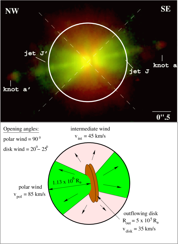
Figure 7: Top panel: HST image of Hen 2-90 replotted with kind permission from Sahai et al. (Sahai02 (2002)). Overplotted is a big circle that indicates the width of the slit (which is 2$\arcsec$, corresponding to 0.019 pc at a distance of 2 kpc) of our Cassegrain observations from which the line luminosities have been derived. Bottom panel: Sketch of the threefold wind derived from the HST image and used in our calculations. Plotted are the outflowing disk, the polar wind, and the intermediate wind. Indicated are also the opening angles of the polar and disk wind used for the model calculations, and the velocities within the different wind regions as derived from Table 1 and discussed in the text. The whole structure is still embedded in an Hii region that extends up to 3$\arcsec$.2 corresponding to 0.031 pc, which is 1.6 times larger than the non-spherical wind structure. The bipolar jet and the knots are not taken into account in the non-spherical wind model.

Based on the HST image of Sahai et al. (Sahai02 (2002), see Fig. 7) we can distinguish three major wind regions: (i) a biconical high-ionization ([Oiii] dominated) polar wind, (ii) a low-ionization ([Nii] dominated) wind at intermediate latitudes which we will call further on the intermediate wind, and (iii) an equatorial outflowing disk. The big white circle indicates the slit width of 2$\arcsec$ of our Cassegrain observations (the flux observed comes from this region). This corresponds to an outer edge of about 0.01 pc at a distance of 2 kpc. The HST resolved structure is embedded into a much larger Hii region with extensions of at least 3$\arcsec$.2 x 3$\arcsec$.1 (Tylenda et al., Tylenda (2003)). Our observations therefore contain neither much contribution of this extended nebula nor from the jets and knots, but are concentrated on the innermost non-spherical wind structure.

The HST image also gives a hint to the location of the different ions. In combination with the velocity information retrieved from the line profiles (Table 1) we can determine the terminal wind velocities of the different regions. For the polar wind we find a mean velocity of $\sim 60$ km s^-1 from the [Oiii] and [Cliii] lines. Taking into account the opening angle of the cone which is about 90$\degr$ and the fact that the system is seen (almost perfectly) edge-on, this results in a terminal velocity of $\sim 85$ km s^-1. For the intermediate wind where the [Siii], [Sii] and [Nii] lines come from, we derive analogously a mean wind velocity of $\sim 45$ km s^-1, and for the disk wind, represented by the [Oi] lines, we find a mean velocity of about 35 km s^-1. The wind velocity shows a latitude dependence being highest in polar directions, and lowest in equatorial direction, the difference is a factor of $\sim 2.5$.

With the adopted distance of 2 kpc we can derive linear scales for the different wind regions from the HST image. The polar wind is visible up to a distance of about $1.5\times 10^{6}$ R_∗ which is slightly beyond our observing slit which only extends to about $1.13\times 10^{6}$ R${}_{*}\simeq 0.01$ pc.

The outer edge of the disk is about $5\times 10^{5}$ R_∗ and we estimate, based on the dark disk-like structure seen on the HST image, a total opening angle of $20-25\degr$.

The remaining volume is filled by the intermediate wind which also shows at its innermost parts indication of a high degree of ionization ([Oiii] dominated). We estimate that this region extends roughly to about $r_{\rm out}$(Oiii)$\simeq 10^{5}$ R_∗.

5.2 The forbidden emission line luminosities

We concentrate our detailed analysis on the forbidden lines. These lines are excellent indicators of the circumstellar material because of two reasons:
(i) They are excited collisionally. Therefore they are very sensitive to the density and temperature.
(ii) The circumstellar nebula is optically thin for these lines, simplifying the analysis.

We model the line luminosities of the forbidden emission lines of Oi, Oii, Oiii, Nii, Clii, Cliii, Ariii, Sii, and Siii present in our spectra (see Table 4). We also find lines from Crii and Criv which we could not model due to the lack of collision parameters, and lots of Feii lines which we also neglect because Feii cannot be treated in such an easy way as the other ions.

The line luminosity of a forbidden line is given by

$$L_{\nu}=\int j_{\nu}(1-W(r))dV$$ (1)

where $j_{\nu}=h\nu N_{\rm i}A_{\rm ij}$ is the line emissivity and $W(r)=\frac{1}{2}(1-\sqrt{1-(R_{*}/r)^{2}})$ is the geometrical dilution factor that accounts for the fraction of photons being intercepted by the star. For the line emissivity we need to calculate the level population. This is done for all the elements cited above by solving the statistical equilibrium equations in a 5-level atom. The collision parameters are taken from Mendoza (Mendoza (1983)) and the atomic parameters from Wiese et al. (Wiese1 (1966), Wiese2 (1969)).

The hydrogen density in a wind follows from the mass continuity equation

$$N_{\rm H}(r)=\frac{\dot{M}}{4\pi r^{2}\mu m_{\rm H}v(r)}$$ (2)

$\dot{M}$ is the mass loss rate of the star and $v(r)$ the wind velocity which is given by a $\beta$-law of the form

$$v(r)=v_{\infty}\left(1-\frac{r_{0}}{r}\right)^{\beta}$$ (3)

with

$$r_{0}=R_{*}\left\{1-\left(\frac{v_{0}}{v_{\infty}}\right)^{\frac{1}{\beta}}\right\}$$ (4)

which sets the velocity at $R_{*}$ equal to the sound velocity ($v_{0}$). $v_{\infty}$ is the terminal velocity in each wind region which has been derived above from the different forbidden lines, and we set $\beta=1$ which is a good approximation for winds of hot stars (Lamers & Cassinelli, Lamers99 (1999)).

The electron density is given in terms of the hydrogen density and depends on the degree of ionization in each part of the wind; in polar direction and in the inner parts of the intermediate wind we set $N_{\rm e}\simeq 1.1\,N_{\rm H}$. In these regions helium is singly ionized contributing about 10% to the total electron density. The contribution from other elements, like O, S, N, which are also (partly twice) ionized, to the total electron density is, however, negligible. For the outer parts of the intermediate wind, where He is assumed to be neutral, we use $N_{\rm e}\simeq 1.0\,N_{\rm H}$ (and neglect again the small contribution from the metals), and for the disk wind, where we assume that hydrogen is neutral, we have only electrons from elements with much lower ionization potential (i.e. lower than about 10 eV). Summing up the number densities of all these elements (assuming solar abundances), results in a maximum electron density in the disk of about $1.3\times 10^{-4}\,N_{\rm H}$. We cannot expect that all possible elements are completely ionized. We therefore use an electron density of $N_{\rm e}\simeq 10^{-4}\,N_{\rm H}$ which is an upper limit to the real disk electron density. Since the excitation of the forbidden lines depends on the electron density, the fitting of the disk lines therefore results in a lower limit of the mass flux, i.e. the disk mass loss rate, because a decrease in electron density needs an increase in total density to account for the observed line luminosities.

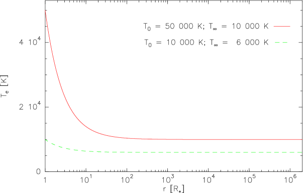
Figure 8: Temperature distribution in the wind according to Eq. (5). The starting values, $T_{0}$, and terminal values, $T_{\infty}$ appropriate for the polar/intermediate wind and for the outflowing disk are indicated. The temperature drops quickly (within 100 R_∗) to its terminal value which is found to be about 10 000 K in the polar and the intermediate wind, and about 6 000 K in the disk wind (see Table 2).

For the temperature distribution we make use of the following equation

$$T(r)=T_{\infty}+(T_{0}-T_{\infty})\left(\frac{r}{R_{*}}\right)^{-x}$$ (5)

Such a temperature distribution has been found by de Koter (deKoter (1993)) to be a reasonable approximation for a wind of a hot star in radiative equilibrium. We set $x=1$, but the value of x does not really influence the results because the forbidden lines are formed in the lower density region, far away from the star, where the temperature has dropped already to its terminal value, $T_{\infty}$ (see Fig. 8). The line luminosities are, however, very sensitive to this terminal temperature.

One additional parameter that needs to be specified is the elemental abundance. Costa et al. (Costa (1993)) have found that the elements are slightly sub-solar in Hen 2-90. However, these values have been derived under the assumption of a spherically symmetric homogeneous nebula which is far from being the case. In addition, Kraus (Kraus (2005)) showed that the abundances when derived using a stellar wind rather than a homogeneous nebula can be much higher. We therefore start our calculations assuming solar abundances (taken from Grevesse & Sauval, Grevesse (1998)) for all elements. Deviations in the calculated line luminosities compared with observations might then be due to individual deviations in the abundances.

5.3 Mass fluxes and total mass loss rate

The results for the ions which are used to restrict the different parameters in our simple, non-spherical wind model are shown in Figs. 9 - 12, where we plotted the line luminosities as a function of $r$, i.e. the volume integrated flux that is achieved in the corresponding wind (i.e. polar, intermediate or outflowing disk) as it would be observed from such a wind with outer edge $r$. For several ions, the observed line luminosities do not come from only one of the three defined winds, but from two different wind regions. Therefore we shortly describe the procedure of how we fitted the different lines.

We started our modeling with the [Siii] 6312Å line (Fig. 9). Since Siii and Oii have about the same ionization potential, it can be expected that no Siii emission will come from regions of Oiii emission. Siii emission is therefore restricted to the intermediate wind at distances from the star, where Oiii, and hence Siv, have recombined already. Therefore, the inner edge of the Siii emission is the outer edge of the Oiii emission, i.e. $r_{\rm in}$(Siii) $=r_{\rm out}$(Oiii) $=10^{5}$ R_∗ as found in Sect. 5.1.

The only free parameters are the temperature distribution and the mass loss rate at these intermediate latitudes. Since the Siii emission region is already rather far away from the star, we assumed the temperature to be constant and found a good fit for $T_{\rm e}\simeq 10\,000$ K. The mass flux of the intermediate wind has been found to be of order $F_{\rm m,int}=1.5\times 10^{-1}$ g s^-1cm${}^{-2}=1.66\times 10^{-6}$ M_⊙yr^-1steradian^-1.

Since Siii has only one prominent forbidden line in our spectral region, this best fit temperature had to be confirmed with the other forbidden lines from the same wind region. Other elements like Nii, Sii and Clii have more than one forbidden line and several line ratios can be used as tracers for the electron temperature. From combining the results from all these temperature indicators the best solution was found to be of order 10 000 K. The valid range of temperatures is very small, and the resulting uncertainty in mass flux is of order 20 %. We want to stress that the dependence of the mass flux on the electron temperature cannot be described with a power law because the collision parameters have a more complicated temperature dependence.

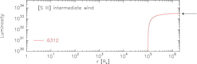
Figure 9: Model results for the [Siii] line arising in the outer parts of the intermediate wind. Shown is the increase in line luminosity with distance from the star. The arrow on the right side of the panel indicates the observed value.

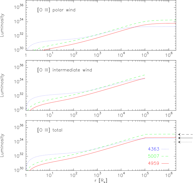
Figure 10: Model results for the different [Oiii] lines listed in the bottom panel. Shown are the individual contributions from the polar and intermediate wind and their line luminosity increase with distance from the star. The bottom panel shows the sum of both contributions, and the arrows on the right side indicate the observed value for each emission line (same line style).

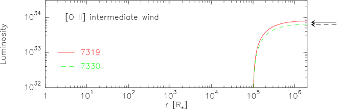
Figure 11: Model results for the [Oii] lines. These lines come from the intermediate wind only, and from distances where Oiii has already recombined (see mid-panel of Fig. 10). The arrows on the right side indicate the observed value for each emission line (same line style).

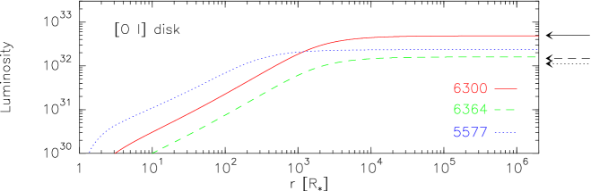
Figure 12: Model results for the [Oi] lines. These lines come from the disk wind only. The arrows on the right side indicate the observed value for each emission line (same line style).

The next element to fit is oxygen and we started with the lines of Oiii. These lines are supposed to come from 2 different regions (see Fig. 7 and Fig. 10): the inner parts of the intermediate wind and the polar wind. To get self-consistent results for all oxygen lines of different ionization state (Figs. 11 and 12), we had to decrease the O abundance from solar to 0.3 solar.

The contribution of the intermediate wind to the [Oiii] lines is restricted to distances within $r_{\rm out}$(Oiii). For the temperature distribution we used $T_{0}=T_{\rm eff}$ and $T_{\infty}=10\,000$ K. The use of the effective stellar temperature as the starting temperature is quite reasonable because the star is supposed to be small where the surface temperature mirrors about the effective temperature. In fact, the choice of the surface temperature does not really affect the behaviour of the line luminosities because the majority of the luminosity comes from the lower density regions where the temperature has reached its terminal value.

Having the contribution from the intermediate wind the remaining line luminosities to the [Oiii] lines must come from the polar wind. Here, the free parameters are again the mass flux and the temperature distribution. We found best agreement by using the same temperature distribution as for the intermediate wind and a polar mass flux of $F_{\rm m,pol}=7.2\times 10^{-2}$ g s^-1cm${}^{-2}=7.99\times 10^{-7}$ M_⊙yr^-1steradian^-1.

With these fixed parameters for the intermediate wind, we found good agreement of observed and modelled [Oii] lines (Fig. 11). The remaining O lines are the [Oi] lines which are assumed to arise in the cool and neutral equatorial disk (Fig. 12). The only constraint for the modeling is the temperature distribution, which should start with a surface temperature around 10 000 K to guarantee that H is neutral. The terminal temperature as well as the disk mass flux could then be fixed by the best fit model (see Fig. 12) to $T_{\infty}=6\,000$ K and $F_{\rm m,disk}=5.5\times 10^{-1}$ g s^-1cm${}^{-2}=6.10\times 10^{-6}$ M_⊙yr^-1steradian^-1.

Table 2: Best fit model parameters for the polar (p), intermediate (i) and disk wind (d). The mass fluxes are assumed to be constant within the indicated $\theta$-ranges and have an error of order 20 %.

	$T_{0}$	$T_{\infty}$	$\theta_{\rm min}$	$\theta_{\rm max}$	$v_{\infty}$	$F_{\rm m}(\theta)$
	[K]	[K]	[$\degr$]	[$\degr$]	[km s-1]	[g s-1cm-2]
p	50 000	10 000	0	45	85	$7.2\times 10^{-2}$
i	50 000	10 000	45	78	45	$1.5\times 10^{-1}$
d	10 000	6 000	78	90	35	$5.5\times 10^{-1}$

All the parameters for the three different wind regions are now fixed and summarized in Table 2. If this picture of the non-spherical wind is about correct, we should be able to fit the luminosities of the remaining forbidden lines (i.e. from Sii, Clii, Cliii, Ariii, and Nii) with the same sets of parameters.

The modeling of the [Sii] lines was rather tricky, because they arise in two different regions: the hydrogen neutral disk and the outer parts of the (ionized) intermediate wind, but with no clear boundary conditions. For the intermediate wind, Sii can only arise if Siii has recombined. The saturation of the [Siii] line luminosities happens at about $10^{6}$ R_∗ (Fig. 9) which is set as the minimum distance for the [Sii] lines. For the emission from the disk the inner edge is set to the stellar surface. A reliable fit is found from the simultaneous fitting of both contributions where we found that the disk contributes less than half to the total emission and that Sii has to recombine at a distance of about 6 000 R_∗. The contribution from the intermediate wind which is more than half of the total line luminosities comes from a very narrow (in radius) region, starting at a distance of about $1.05\times 10^{6}$ R_∗ just beyond the region of Siii line luminosity saturation and extending to the edge of our slit which is at $1.13\times 10^{6}$ R_∗. Since the line luminosities from the intermediate wind did not saturate at the outer edge of our slit, we expect the [Sii] lines to appear much more luminous when observed with a larger slit width.

The predicted line luminosities of the nitrogen lines were much too high so that we had to reduce the N abundance to $0.5\times$ solar to achieve good fits.

In Table 3 we summarize all the observed (column 3) and modelled (column 4) line luminosities, as well as the ratio of observed over modelled luminosity (column 5) and the location(s) of the ions in either the polar wind (p), intermediate wind (i) or disk (d) or a combination of two. We thereby distinguish two sets of lines: the lines which are used to derive the mass fluxes and temperature distributions in the different wind regions are collected in the upper part, and the lines that are used for confirmation of the models and for derivation of the abundance (especially of N) are given in the lower part.

Table 3: Observed and modelled forbidden line luminosities. For the observed values, we took the intensities given in Table 4 and assumed a distance of 2 kpc. The fifth column contains the ratio of observed over modelled line luminosity and in the sixth column we describe in which part(s) of the wind the line is produced: The classifications of p, i, and d mean polar wind, intermediate wind, and disk, respectively. We gathered in the upper part the lines which are used to derive the mass fluxes and temperature distributions in each wind zone while the lines in the lower part have been used to confirm the models and to derive (in the case of N) the abundance.

Ion	$\lambda$ (Å)	$L_{\lambda}^{\rm obs}$	$L_{\lambda}^{\rm model}$	ratio	region
Oiii	4363	$9.71\times 10^{33}$	$2.90\times 10^{34}$	0.33	p,i
Oiii	4959	$3.58\times 10^{34}$	$3.91\times 10^{34}$	0.92	p,i
Oiii	5007	$1.13\times 10^{35}$	$1.13\times 10^{35}$	1.00	p,i
Oii	7319	$7.23\times 10^{33}$	$7.70\times 10^{33}$	0.94	i
Oii	7330	$6.18\times 10^{33}$	$6.17\times 10^{33}$	1.00	i
Oi	5577	$1.12\times 10^{32}$	$2.33\times 10^{32}$	0.48	d
Oi	6300	$4.98\times 10^{32}$	$4.86\times 10^{32}$	1.02	d
Oi	6364	$1.49\times 10^{32}$	$1.60\times 10^{32}$	0.93	d
Siii	6312	$2.95\times 10^{33}$	$2.98\times 10^{33}$	0.99	i
Sii	4068	$1.15\times 10^{33}$	$4.57\times 10^{32}$	2.52	i,d
Sii	4076	$3.43\times 10^{32}$	$1.18\times 10^{32}$	2.90	i,d
Sii	6716	$9.05\times 10^{31}$	$1.05\times 10^{32}$	0.86	i,d
Sii	6731	$2.13\times 10^{32}$	$2.20\times 10^{32}$	0.97	i,d
Nii	5755	$4.56\times 10^{33}$	$4.57\times 10^{33}$	1.00	i
Nii	6548	$4.84\times 10^{33}$	$6.15\times 10^{33}$	0.79	i
Nii	6584	$2.08\times 10^{34}$	$1.81\times 10^{34}$	1.15	i
Cliii	5517	$1.10\times 10^{32}$	$4.23\times 10^{31}$	2.60	p,i
Cliii	5538	$1.74\times 10^{32}$	$1.74\times 10^{32}$	1.00	p,i
Clii	6153	$3.88\times 10^{31}$	$3.82\times 10^{31}$	1.01	i
Ariii	5193	$1.16\times 10^{32}$	$6.44\times 10^{32}$	0.18	p,i
Ariii	7136	$7.37\times 10^{33}$	$6.88\times 10^{33}$	1.07	p,i
Ariii	7753	$1.49\times 10^{33}$	$1.68\times 10^{33}$	0.89	p,i

Inspecting Table 3 shows that some of the modelled lines can be off by a factor of 2 or larger. Here, we want to give some arguments that might explain these differences.

1. We start with the [Oi] line at $\lambda=5577$ Å for which our model predicts about twice as much luminosity than observed. This line corresponds to the transition $5\longrightarrow 4$ in our adopted 5-level atom. There exists one permitted transition between its upper level and a much higher level with wavelength $\lambda=1217.6$ Å which falls into the wavelength range covered by a broadened Ly $\alpha$ line ($\lambda_{\rm Ly\,\alpha}=1215.6$ Å). The fifth level might therefore be depopulated radiatively into this higher state from which several permitted lines arise, and the observable 5577 Å line luminosity will decrease.

2. An important source of error might be the foreground extinction used to de-redden our data. We took the foreground extinction value from Costa et al. (Costa (1993)) who derived it from the Balmer lines which they assumed to arise in a spherically symmetric constant density nebula. Since some of the modelled line luminosities arising in the blue part of the spectrum (at $\lambda<5000$ Å) are off compared to the observed luminosities, it seems that this might be a systematical error rather than a model error. However, our modeling procedure is not suitable to derive the real extinction value. A slightly different extinction will certainly result in slightly different model parameters, e.g. the mass fluxes in the different wind regions will change individually. This makes it difficult to predict in which way the extinction might be off, especially since some of the forbidden lines arise in two different regions and have to be fitted simultaneously, as e.g. the [Sii] lines. Nevertheless, de-reddening with the correct extinction value is especially important if we have to compare lines from the same ion arising in the very blue part of the spectrum with lines coming from the very red part of the spectrum, which is the case e.g. for the lines of Ariii where we have a deviation of the blue line with respect to the red lines by a factor of 5!

3. An additional reason for the deviations might be the accuracy of the measured line fluxes coming from different wavelength regions. As explained in Sect. 2, the line fluxes from the high and low wavelength regions, i.e. at wavelengths $\lambda<5000$ Å and $\lambda>7000$ Å have much larger uncertainties due to the lower S/N ratio and efficiency of the CCD leading to larger errors in the measured line fluxes.

Except of the [Oi] 5577 Å line we think that both effects, a slightly different foreground extinction and a larger uncertainty in the measured line fluxes, play a role but it is difficult to disentangle the individual influence of these effects on a certain line.

From the results presented in Table 2 for the different wind parts it is obvious that the mass flux varies with latitude being lowest at the poles and highest at the equator with $F_{\rm m,disk}\simeq 8\,F_{\rm m,pole}$. The total mass loss rate of the star is given by the integral of the mass flux over the stellar surface which is

$$\dot{M}=4\pi R_{*}^{2}\int\limits_{0}^{\pi/2}F_{\rm m}(\theta)\sin\theta d\theta$$ (6)

Inserting our values given in Table 2 we find a total mass loss rate of the star of $\dot{M}\simeq(2.9\pm 0.6)\times 10^{-5}\,{\rm M}_{\odot}{\rm yr}^{-1}$. The error results from the uncertainties in mass flux.

5.4 The wings of H$\alpha$

With this complete wind scenario derived in the previous section we can return to the question whether the broad wings of the H$\alpha$ line are due to outflow or electron scattering. From our data we derive a contribution of about 10% of the broad wings to the total intensity which implies an electron scattering optical depth of about 0.09 in and above the line formation region of H$\alpha$. On the other hand, we can calculate the electron optical depth from

$$\begin{array}[]{l}\tau_{e}=\int N_{e}(r)\sigma_{e}dr\end{array}$$ (7)

where $N_{e}(r)$ is the electron density distribution in the line of sight between the observer and the formation region of the line, and $\sigma_{e}$ is the electron scattering coefficient. Since we see Hen 2-90 more or less edge-on, we can use the electron density distribution from the intermediate wind and calculate backwards, i.e. from the observer into the wind, to determine where in the wind most of the H$\alpha$ emission is produced. For our intermediate wind electron density distribution and the optical depth of 0.09 we find that the majority of the H$\alpha$ emission arises within about 4000 R_∗ around the star which is the region of highest density and therefore the most plausible location. We can therefore state that the wings of H$\alpha$ are indeed produced due to electron scattering and not due to a high velocity wind.

Additional confirmation of the broadening due to electron scattering rather than due to high velocity outflow is provided by our wind scenario proposed above. Our non-spherical wind model covers the complete surrounding of the star except of the highly-collimated jets which have been found to have real outflow velocities of less than 400 km s^-1 (see e.g. Sahai et al., Sahai02 (2002)). What we found from our wing velocity measurements in all the different parts of the wind is: a terminal outflow velocity of about 85 km s^-1 from the [Oiii] lines in the polar wind, of about 40 km s^-1 from the [Nii] and [Siii] lines in the intermediate wind, and about 35 km s^-1 from the [Sii] and [Oi] lines in the disk. We could not identify any additional wind component which might have an outflow velocity as high as 1800 km s^-1.

6 Discussion

6.1 The non-spherical wind scenario for Hen 2-90

For the model calculations we use the geometry and ionization structure based on the HST image (Fig. 7) which clearly shows a polar wind, an intermediate wind and disk so that the geometry used seems to be well justified.

Such a non-spherical wind model with latitude dependent temperature, terminal wind velocity, and mass flux might be understood in terms of a rotating star. According to the van Zeipel theorem, rapid rotation will lead to polar brightening. This means that the surface temperature of the star can be much hotter on the pole compared to the equator. Our calculations show that in equatorial regions the surface temperature should not be higher than about 10 000 K to guarantee that hydrogen is neutral. In polar directions we found that the terminal temperature should not be lower than about 10 000 K which means that the surface temperature can be much hotter. We do not have a good handle on the real polar surface temperature because the forbidden emission lines are produced far away from the star where the temperature dropped already to its terminal value. In our calculations we used the effective temperature of 50 000 K found by Kaler & Jacoby (Kaler (1991)) with the Zanstra method. Cidale et al. (Cidale (2001)) derived a much lower effective temperature of only 32 000 K using the energy balance method. We tested our model for different polar surface temperatures in the range $T_{0}=15\,000-50\,000$ K. We found, that for different surface temperatures large differences occur in the line luminosities close to the star. However, in the regions of our interest, where the lines saturate, the line luminosities are all about equal. This implies that from our observations we cannot draw any conclusion on the real polar surface temperature.

Rotation not only influences the surface temperature structure, but also the terminal wind velocities resulting in a decrease in terminal velocity from pole to equator (see e.g. Lamers & Cassinelli, Lamers99 (1999); Kraus & Lamers, Kraus05 (2005)). This is exactly what we found from our observations, when we take into account the known inclination of the system as suggested from the HST image.

The ratio of polar (85 km s^-1) to disk terminal velocity (35 km s^-1) of about 2.4 derived from the forbidden emission lines is consistent with a rotation speed of about 75 – 80 % of the critical velocity (Kraus & Lamers, Kraus05 (2005)). Such high velocities are observed e.g. for the classical Be stars (see e.g. Porter & Rivinius, Porter (2003)). Some of those stars have recently been suggested to rotate even close to break-up, i.e. with almost critical velocity (Townsend et al., Townsend (2004)).

An additional effect of rotation is that it leads to a latitude dependent mass flux which is also the case for Hen 2-90. A mechanism like the wind compressed disk (Bjorkman & Cassinelli, Bjorkman (1993)) or the rotation induced bistability (Lamers & Pauldrach, Lamers91 (1991)), or a combination of both can result in the observed high density equatorial outflowing disk.

The combination of the latitude dependent mass flux and surface temperature also explains why we see different ionization structures at different latitudes. The lower surface temperature results in less ionizing UV photons, and the higher mass flux into a higher shielding density which in summary reduces the degree of ionization.

For our model calculations the outflowing disk is assumed to be neutral in hydrogen. Kraus & Lamers (Kraus03 (2003)) showed that in the case of supergiants the disk created by an equatorial wind can indeed become neutral just above the stellar surface if the equatorial mass flux is high enough to prevent ionizing stellar photons from penetrating into the high density equatorial disk wind. Although Hen 2-90 is hotter than a typical supergiant (but its effective temperature might well be only 32 000 K instead of 50 000 K as stated above), it has also a much smaller radius leading to an enormous equatorial mass flux whose material is indeed dense enough to shield the disk material efficiently from stellar irradiation. Consequently, the disk will stay neutral even close to the stellar surface.

The terminal temperature found for the gas disk is about 6 000 K. From our modeling we found that the luminosities of the forbidden lines coming from the disk saturate at a distance of about $2\times 10^{4}$ R_∗. The total size of the disk is, however, much larger, at least $5\times 10^{5}$ R_∗. The ISO spectrum of Hen 2-90 shows a strong IR excess due to hot circumstellar dust which can only be located in the disk. The evaporation temperature of dust is between 1 500 K and 2 000 K, depending on its composition. In the temperature region between the atomic and the dust dominated regions, the atoms might be locked into molecules that can form (and survive) at temperatures below about 5 000 K. Our results are therefore also consistent with a circumstellar dust disk where the dust forms far away from the star, at distances $r_{\rm dust}\gg 2\times 10^{4}$ R${}_{*}\simeq 35$ AU. A detailed study of the ISO spectrum to calculate the infrared emission coming from the predicted dust disk is necessary and currently under investigation (Borges Fernandes & Lorenz-Martins, in preparation).

It would be interesting to see whether the ionization structure we found from our modeling of the forbidden emission lines might be reproduced by more sophisticated ionization structure calculations in such a non-spherically symmetric wind scenario. Unfortunately, as far as we know, there exist no numerical codes to perform the necessary 3D radiation transfer needed for non-spherical ionization structure calculations.

Finally, we qualitatively discuss how the variety of the line profiles, shown in Sect. 3, might be produced in our non-spherical wind scenario. Even though the central star might be rapidly rotating, we do not think that (especially the double peaked) line profiles mirror the stellar rotation or are due to rotation at all (although we cannot ad hoc exclude a rotational contribution) because the effective temperature of about 50 000 K indicates, that the star must have a line-driven wind. The acceleration of the wind to its terminal velocity happens within only a few stellar radii, leading to a radially outflowing wind.

Double-peaked lines: these lines are mainly produced in the intermediate wind (some of them with a gaussian contribution from the polar wind) which can be regarded as a thick expanding torus. Since we see this torus edge-on, the emission lines formed within it show double-peaked profiles. Since the maximum (terminal) wind velocity of the intermediate wind is about 45 km s^-1, the peak separation will be of order 40 to 50 km s^-1, what is observed.

Broad single-peaked lines: they are found for the hydrogen Balmer lines. As discussed already in Sect. 5.4, the broad wings of H$\alpha$ are due to electron scattering with a scattered intensity of about 10%. With increasing quantum number, the Balmer line intensities decrease and a 10% contribution in the broad wings becomes much harder to detect above the continuum. That’s why with increasing quantum number the derived wing velocities of the Balmer lines decrease until they adapt to the terminal wind velocities derived from the forbidden lines (see e.g. line H8 in Table 1).

Narrow single-peaked lines: these lines are mainly formed in the disk (even though some of them can have small contributions from the intermediate wind). The lines formed in the outflowing edge-on seen disk should also show double-peaks as the lines formed in the intermediate wind. However, since the disk outflow velocity is smaller than the velocity in the intermediate wind, the two peaks merge leading to a single-peaked line profile.

The variety of profiles observed can be explained with our model assumptions. However, we have no explanation for the asymmetric line profiles with a strong red peak. Probably, our scenario is not completely correct, and effects like clumping in the wind might be worth being investigated.

A quantitative analysis of the line profiles would be necessary, but this is with our data difficult and beyond the scope of this paper, because the profiles are derived from the FEROS spectrum which is not flux calibrated, while the line luminosities have been derived from the low-resolution Cassegrain spectrum, which makes it impossible to model line luminosities and profiles simultaneously.

6.2 Hen 2-90: a symbiotic object or a compact planetary nebula ?

In the literature Hen 2-90 has been classified either as a (compact) planetary nebula (e.g. Costa et al., Costa (1993); Maciel, Maciel (1993); Lamers et al., Lamers98 (1998)) or as a symbiotic object, i.e. a binary consisting of a cool giant and a hot component with an accretion disk (Sahai & Nyman, Sahai00 (2000); Guerrero et al., Guerrero (2001)).

The HST image (Fig. 7, Sahai et al., Sahai02 (2002)) clearly shows the presence of a nebula bisected by a disk, with a highly collimated and bipolar jet with several pairs of knots at both sides. This scenario could be explained assuming that Hen 2-90 is either a compact planetary nebula, where the wind asymmetries started during the AGB phase, or a binary system, where the jets are caused by an accretion disk.

During our modelling procedure we have found, as also cited by Costa et al. (Costa (1993)) and Maciel (Maciel (1993)), a depletion of N and O by a factor of 2 and 3.3, respectively, with respect to the electron density with S, Ar and Cl having normal (i.e. solar) abundances. In addition, the FEROS spectrum contains only one single permitted carbon line, Cii $\lambda$6578. This line has previously been detected by Costa et al. (Costa (1993)) and Guerrero et al. (Guerrero (2001)), but it is very weak in the FEROS spectrum (just at the detection limit) and absent in the Cassegrain spectrum. We can only estimate its line flux and we found about 0.06 for the observed flux, and about 0.02 for the dereddened flux in the scaling of Table 4 (H$\beta=100$). The uncertainty of these line fluxes is about 50%. No forbidden emission line of carbon was detected, even though in the optical spectrum we would expect to observe several [Ci] lines coming from the disk. We applied our disk wind model to calculate the line luminosities for these carbon lines, and found that these lines would only show up in the spectrum for a carbon abundance of at least twice solar. Inspection of the ISO spectrum of Hen 2-90 reveales emission from oxygen-rich dust (Borges Fernandes & Lorenz-Martins, in preparation). Oxygen-rich dust can only be the dominant dust component in case ${\rm O/C}>1$ during the ejection time of the dust forming material. We found an underabundance of O by more than a factor of 3. Together with the fact that the dust composition should mirror the actual wind composition (unless the star has changed its composition from O-rich to C-rich since the ejection of the dust forming material, which is rather unlikely), we conclude that (i) the progenitor star that ejected the dust forming material cannot have been carbon rich, and (ii) the actual carbon abundance must be less than 0.6 solar to guarantee ${\rm O/C}>1$. Assuming a standard scenario with dredge-ups, we can understand the depletion of C and O, however, we have no explanation for the fact that N is also depleted. There are some B-type post-AGB stars in the halo of our Galaxy showing the same behaviour (Moehler & Heber, Moehler (1998)), and recently Lennon et al. (Lennon (2004)) reported on a Be star with an unexpected low N abundance. However, the origin of those anomalies is still poorly understood. Rotation or a possible binarity could play an important role. Unfortunately, as far as we know, there exist no stellar evolution models that follow the whole life sequence of rapidly rotating intermediate mass stars, for which Hen 2-90 seems to be a candidate.

Another point that should be commented is that from our spectra, that cover the complete optical wavelenght range, we have identified no lines from ions with ionization potential higher than $\sim 40$ eV and consequently no He ii lines. In addition, there is no indication for the presence of TiO bands either. These two characteristics are the main signature of a symbiotic system. Since we see the disk of Hen 2-90 almost edge-on it might be possible that the disk hides the atmosphere of a cool giant, where the TiO bands are formed, and also absorb the He ii emission from a hot component. However, the fact that we don’t see hints for any other line from ions with ionization potential higher than $\sim 40$ eV leads us to the conclusion that these ions (and therefore also He ii) do not exist in the wind of Hen 2-90 indicating that (i) the effective temperature of Hen 2-90 is indeed much lower than the 50 000 K found from the Zanstra method and may well be of order 32 000 K as derived by Cidale et al. (Cidale (2001)) from the energy balance, and (ii) the symbiotic system is not the favoured classification.

Besides the absence of clear indications for a classification as a symbiotic object, our results favour the conclusion of Hen 2-90 being a compact planetary nebula and we want to mention two more features that support this idea:

1. The mass loss rate of $\sim 3\times 10^{-5}$M_⊙yr^-1 found for Hen 2-90 coincides with those found for proto-planetary nebulae with axially symmetric dust shells resulting from a so-called superwind (see e.g. Meixner et al., Meixner (1997)).

2. An observational curiosity in the spectrum of Hen 2-90 is the fact that the [Oiii] 5007 Å line is less intense than the H$\alpha$ line, although for a compact planetary nebula it is usually the other way round. However, in our forbidden line analysis we found that the abundance of O had to be reduced to only 0.3 solar to achieve reasonable line luminosity fits. This means, that if Hen 2-90 had a ‘normal’ O abundance, the 5007 Å line would be about 3.3 times stronger than observed, and consequently be higher than the H$\alpha$ flux. The anomalous line flux is therefore due to the underabundance of O.

We cannot definitely exclude a binary nature of Hen 2-90 (see also the discussion in Kraus et al., Krausetal05 (2005)). Unfortunately, the optical continuum of Hen 2-90 is completely flat, making it impossible to disentangle individual components. In addition, the optical continuum is mainly due to free-free and free-bound emission in the optically thick wind, rather than by the stellar continuum.

Observed features, that might hint to a binary nature, are the jet-like structure with blob ejections (Sahai, Sahai (2002); Sahai et al., Sahai02 (2002)), and the DENIS NIR photometry cited by Guerrero et al. (Guerrero (2001)):

Jet-like structure and blob ejection: The jet structure seen in Hen 2-90 is very collimated, and the blobs are found to be ejected regularly on a 40 year timescale. This perfect alignment of the jet axis and the blobs is unique. All PNe which are known to be binaries show either asymmetric or point-symmetric jet and blob ejection. In addition, to date no X-ray emission coming from an accretion disk has been detected from the system which might indicate a completely different formation mechanism. Garc$\acute{\rm\i}$a-Segura et al. (Garcia (2001)) modeled the jet and knots of Hen 2-90 using the concept of magnetohydrodynamics in the wind of a single star and under the assumption of a solar-like magnetic cycle. This model does not need a binary for the jet production, because the jet formation is not driven by an accretion disk. A binary component might be helpful in the first instance, to spin-up the star to high rotation rates (e.g. in a merger process) and, therefore, to increase the stellar magnetic field to the values needed for their model calculations. Such a spin-up might also explain the high rotation velocity of the central star which we claimed in the previous section and derived from the observed terminal velocities.

DENIS NIR photometry: Schmeja & Kimeswenger (Schmeja (2001)) used the new DENIS survey data to probe different types of PNe. Their Fig. 1 shows a distinction between genuine PNe, symbiotic Miras and IR-[WC] PNe on the basis of a colour-colour plot. With the published DENIS photometry data of Hen 2-90 (Schmeja & Kimeswenger, Schmeja2 (2002)), and corrected for the extinction value of Costa et al. (Costa (1993)), Hen 2-90 falls into the intermediate region between the genuine PNe and the IR-[WC] PNe. However, the IR-[WC] PNe are supposed to have strong PAH emission which increases their K-band flux and shifts them off the genuine PNe region. A pollution of the K band emission might also be present for Hen 2-90 which shows a huge zoo of emission features in the IR. Subtraction of this polluting emission might shift Hen 2-90 back into the regime of the genuine PNe. In addition, the carbon abundance found for Hen 2-90 is way too small to classify it as a carbon rich star.

From our observations, modeling and the above discussion we conclude that Hen 2-90 must be at least an evolved and probably rapidly rotating object, and the classification as a compact planetary nebula seems to be favourable. The question whether this compact planetary nebula is part of a binary system can only be solved if clear direct indications of a companion star are observed, which is up to now not the case but makes it worth looking at this object in much more detail.

7 Conclusions

In this paper we studied the non-spherical mass loss history of Hen 2-90 by splitting the analysis into a qualitative and a quantitative part.

In the first part, we presented high and low resolution optical observations of the innermost non-spherical wind structure around Hen 2-90. The spectra contain a huge number of forbidden and permitted emission lines of different ionization states justifying the classification of Hen 2-90 as an object showing the B[e] phenomenon. The emission lines can be separated into four groups according to the different shape of their profiles: broad and narrow single-peaked lines, double-peaked lines, and lines with a well pronounced shoulder. This variety of line profiles indicates a complex structure of the circumstellar medium. There are no absorption lines present in the spectrum.

In the second part of the paper we performed a detailed analysis of the forbidden emission lines. The wind geometry used is based on the HST image which reveals a non-spherical wind structure consisting of a polar wind, an outflowing disk and an intermediate wind in between these two (see Fig. 7). In all three parts, the ionization structure is different, indicating a latitude dependence of the surface temperature and the mass flux. These assumptions could be confirmed by our forbidden line analysis and might be interpreted in terms of a rapidly rotating (75 – 80% critical) underlying star. We could determine mass fluxes of $0.07\pm 0.01$ g s^-1cm^-2, $0.15\pm 0.03$ g s^-1cm^-2, and $0.55\pm 0.11$ g s^-1cm^-2 (i.e. $7.99\times 10^{-7}$ M_⊙yr^-1steradian^-1, $1.66\times 10^{-6}$ M_⊙yr^-1steradian^-1, and $6.10\times 10^{-6}$ M_⊙yr^-1steradian^-1) for the polar, intermediate and disk wind, respectively. The surface temperature might change from 50 000 K – 32 000 K (or less) at the pole to about 10 000 K at the equator, and the terminal velocities are 85 km s^-1 (polar wind), 45 km s^-1 (intermediate wind) and 35 km s^-1 (disk). The total mass loss rate is found to be $(2.9\pm 0.6)\times 10^{-5}$ M_⊙yr^-1.

From the almost absence of observable carbon lines in our spectra and from the fact that Hen 2-90 shows clearly O-rich dust in the ISO spectrum, we could restrict the C abundance to a value less than about 0.6 solar. In addition we found that the O abundance is 0.3 solar and the N abundance is about 0.5 solar leading to an enhanced N/O ratio of 5/3 with respect to the solar value, while Ar, S and Cl could be modelled with solar abundances. The depletion of C and O follow from stellar evolution, but for the depletion of N we have no satisfying explanation; it cannot be explained by a standard stellar evolution scenario with dredge-ups.

From our observations and modeling results we can conclude that Hen 2-90 must be an evolved object with most probably a rapidly rotating central star and we favour the interpretation of Hen 2-90 being a compact planetary nebula. Whether it is part of a binary system is still an unsolved question. More observations and better evolutionary models for rapidly rotating stars are certainly needed for a better comprehension of this really curious object.

Table 4: Emission line intensities relative to H$\beta$ = 100 obtained with B&C spectrograph.

Wavelength (Å)	Iobs($\lambda$)	Icorr($\lambda$)	Identification
3833.8	3.14	12.88	H9 3835.4
3867.1	1.67	6.37	He i (m20) 3867.5
3887.5	7.20	26.22	He i (m2) 3888.7
			H8 3889.1
3968.6	6.06	20.37	H$\epsilon$ 3970.1
4025.5	1.15	3.48	He i (m18) 4026.2
4068.0	0.95	1.78	S ii [m1F] 4068.6
4075.8	0.33	0.53	S ii [m1F] 4076.2
4101.4	11.24	33.26	H$\delta$ 4101.7
4120.5	0.19	0.45	O ii (m20) 4119.2
			O ii (m20) 4120.3
			O ii (m20) 4120.6
			He i (m16) 4121.0
			S ii (m2) 4121.0
4143.8	0.30	0.85	He i (m53) 4143.8
4178.8	0.23	0.41	Fe ii (m28) 4178.9
			Fe ii [m21F] 4177.2
			Fe ii [m23F] 4179.0
4233.4	0.12	0.17	Fe ii (m27) 4233.2
4245.0	0.14	0.26	Fe ii [m21F] 4244.8
4288.0	0.20	0.38	Fe ii [m7F] 4287.4
4341.3	24.40	54.89	H$\gamma$ 4340.5
4364.0	4.12	15.03	O iii [m2F] 4363.2
4388.6	0.51	0.99	He i (m51) 4387.9
4416.3	0.46	0.83	Fe ii (m27) 4416.8
			Fe ii [m6F] 4414.5
			Fe ii [m6F] 4416.3
4472.7	3.68	6.68	He i (m14) 4471.7
4490.9	0.08	0.21	Fe ii [m6F] 4488.8
			Fe ii (m37) 4491.4
4520.8	0.26	0.36	Fe ii (m37) 4520.2
			Fe ii (m38) 4522.6
4554.3	0.23	0.38	S iii (m2) 4552.7
4584.7	0.22	0.33	Fe ii (m37) 4582.8
			Fe ii (m38) 4583.8
			Fe ii (m26) 4584.0
4596.3	0.16	0.22	Fe ii (m37) 4595.7
4608.1	0.23	0.37	N ii (m5) 4607.2
4630.8	0.17	0.27	Fe ii (m37) 4629.4
			N ii (m5) 4630.5
4641.7	0.11	0.20	N iii (m2) 4640.6
			O ii (m1) 4641.8
			N iii (m2) 4641.9

Table 4: (continued)

Wavelength (Å)	Iobs($\lambda$)	Icorr($\lambda$)	Identification
4659.3	3.62	4.31	Fe iii [m3F] 4658.1
4702.4	1.51	1.92	Fe iii [m3F] 4701.5
4713.5	0.81	1.05	He i (m12) 4713.4
4734.4	0.71	0.86	Fe ii (m43) 4731.4
4755.4	0.59	0.70	Fe iii [m3F] 4754.7
4770.6	0.62	0.80	Fe iii [m3F] 4769.4
4778.3	0.41	0.51	S ii (m8) 4779.1
			N ii (m20) 4779.7
4815.3	0.09	0.09	Fe ii [m20F] 4814.6
4861.7	100.00	100.00	H$\beta$ 4861.3
4881.3	0.16	0.19	Fe iii [m2F] 4881.0
4904.8	0.20	0.23	Fe ii [m20F] 4905.4
4922.5	1.72	1.97	He i (m48) 4921.9
			Fe ii (m42) 4923.9
4930.5	0.42	0.43	Fe iii [m1F] 4930.5
4959.0	63.49	55.37	O iii [m1F] 4958.9
5001.1	0.32	0.26	N ii (m19) 5001.1
5006.8	182.80	149.08	O iii [m1F] 5006.9
5011.3	2.18	1.78	Fe iii [m1F] 5011.3
5015.7	4.22	3.45	He i (m4) 5015.7
5018.4	0.28	0.23	Fe ii (m42) 5018.4
5041.4	0.60	0.43	Si ii (m5) 5041.1
5047.6	0.30	0.17	S ii (m15) 5047.3
5055.8	0.56	0.30	Si ii (m5) 5056.4
5084.4	0.21	0.19	Fe iii [m1F] 5084.8
5158.9	0.31	0.21	Fe ii [m18F] 5158.0
5168.1	0.26	0.18	Fe ii (m42) 5169.0
5191.6	0.35	0.18	Ar iii [m1F] 5193.3
5197.9	0.57	0.28	Fe ii (m49) 5197.6
5233.9	0.36	0.26	Fe ii (m49) 5234.6
5270.2	3.94	2.93	Fe iii [m1F] 5270.4
5316.3	0.73	0.40	Fe ii (m49) 5316.6
5332.7	0.27	0.10	Fe ii [m19] 5333.7
5363.0	0.29	0.15	Fe ii (m48) 5362.9
			Fe ii [m17F] 5362.1
5375.1	0.13	0.06	Fe ii [m19F] 5376.5
5411.5	0.41	0.21	Fe iii [m1F] 5412.0
5425.4	0.12	0.05	Fe ii (m49) 5425.3
5432.2	0.12	0.04	Fe ii (m55) 5432.9
			Fe ii [m18F] 5433.2
5475.6	0.26	0.05	Fe ii (m49) 5477.7
5505.4	0.26	0.06	Cr iii [m2F] 5505.1
5517.6	0.56	0.17	Cl iii [m1F] 5517.2
5535.5	0.71	0.27	Cl iii [m1F] 5537.7

Table 4: (continued)

Wavelength (Å)	Iobs($\lambda$)	Icorr($\lambda$)	Identification
5551.3	0.43	0.10	N ii (m63) 5552.5
5577.7	0.08	0.02	O i [m3F] 5577.4
5665.9	0.20	0.08	N ii (m3) 5666.4
5677.8	0.39	0.16	N ii (m3) 5676.0
5713.5	0.36	0.11	Fe ii [m2F] 5713.4
5754.5	12.16	7.06	N ii [m3F] 5754.8
5875.2	30.46	13.93	He i (m11) 5875.6
5956.8	0.47	0.21	Si ii (m4) 5957.6
5978.8	0.79	0.33	Si ii (m4) 5979.0
5999.8	0.35	0.12	Ni iii 6000.2
6095.8	0.12	0.03	S ii (m13) 6097.1
6124.5	0.23	0.06	S ii (m13) 6123.4
6152.5	0.26	0.06	Cl ii [m3F] 6152.9
6248.4	0.29	0.07	Fe ii (m74) 6247.6
6300.4	1.93	0.77	O i [m1F] 6300.2
6312.0	12.84	4.57	S iii [m3F] 6311.9
6347.1	1.06	0.35	Si ii (m2) 6347.1
6364.0	0.67	0.23	O i [m1F] 6363.9
6371.4	0.72	0.25	Fe ii (m40) 6369.5
			Si ii (m2) 6371.4
6384.6	0.55	0.16	Fe ii 6383.8
6401.4	0.26	0.07	Ni iii 6401.5
6456.6	0.30	0.08	Fe ii (m74) 6456.4
6483.2	0.17	0.05	Uid
6492.3	0.31	0.09	Fe ii 6493.1
6516.9	0.12	0.03	Fe ii (m40) 6516.1
6533.3	0.25	0.08	Ni iii 6533.9
6548.1	26.90	7.49	N ii [m1F] 6548.1
6563.0	1200.00	317.53	H$\alpha$ 6562.8
6583.6	120.00	32.15	N ii [m1F] 6583.6
6678.0	10.29	3.08	He i (m46) 6678.2
6716.2	0.51	0.14	S ii [m2F] 6716.4
6730.5	1.25	0.33	S ii [m2F] 6730.8
6746.9	0.15	0.04	Cr iv [m2F] 6746.2
6793.3	0.13	0.04	Fe i 6793.3
6826.9	0.15	0.03	Fe iii 6826.2
6895.2	0.14	0.04	Fe ii [m14F] 6896.2
6914.8	0.57	0.14	Cr iv [m2F] 6915.6
6944.9	0.15	0.03	Fe ii [m43F] 6944.9
6996.2	0.31	0.07	[Fe iv] 6997.1
7001.9	0.14	0.03	O i (m21) 7001.9
7064.0	16.03	3.74	He i (m10) 7065.2
7087.3	0.11	0.03	Cr iv [m2F] 7087.1
7109.7	0.19	0.05	Uid

Table 4: (continued)

Wavelength (Å)	Iobs($\lambda$)	Icorr($\lambda$)	Identification
7134.3	50.46	11.41	Ar iii [m1F] 7135.8
7154.2	0.32	0.07	Fe ii [m14F] 7155.1
7169.2	0.21	0.05	Fe ii [m14F] 7171.9
7181.8	0.10	0.02	Fe ii (m72) 7181.2
7232.9	0.74	0.14	Cr iv [m1F] 7233.4
7253.1	0.39	0.07	O i (m20) 7254.2
7279.7	2.03	0.41	He i (m45) 7281.4
7296.2	0.16	0.03	Uid
7317.9	57.34	11.19	O ii [m2F] 7318.6
7328.2	48.95	9.56	O ii [m2F] 7329.9
7375.8	0.31	0.06	Fe ii 7376.5
7388.5	0.42	0.08	Fe ii [m14F] 7388.2
7409.6	0.15	0.03	Si i (m23) 7409.1
7422.6	0.13	0.02	[Fe iii] 7422.6
7431.2	0.27	0.04	Fe ii 7431.35
7449.2	0.22	0.02	Fe ii (m73) 7449.3
			Fe ii [m30F] 7449.6
7465.8	0.23	0.03	Ni i [m2F] 7464.4
7478.1	0.13	0.02	Fe i 7478.9
7498.0	0.54	0.08	Fe ii [m3F] 7497.7
7514.1	0.45	0.07	Fe ii (m73) 7515.9
7712.2	0.59	0.10	Fe ii [m30F] 7710.8
7751.0	14.91	2.30	Ar iii [m1F] 7753.2
7775.1	0.46	0.08	O i (m1) 7775.4
7817.2	0.56	0.09	He i (m69) 7816.2
7868.9	0.42	0.05	Uid
7892.5	2.16	0.32	Uid
7917.8	0.82	0.10	Fe ii [m29F] 7916.9
8131.6	0.34	0.04	Uid
8184.4	0.38	0.05	N i (m2) 8184.8
8309.7	0.19	0.02	Cr ii [m1F] 8308.7
8317.6	0.24	0.03	Uid
8335.0	0.33	0.04	P24 8334.0
8345.7	0.50	0.05	P23 8346.0
8357.5	0.67	0.08	P22 8359.0
8372.9	1.22	0.14	Uid
8388.1	0.77	0.09	Uid
8406.4	0.83	0.09	Uid
8428.5	1.24	0.12	Uid
8453.6	1.01	0.11	Uid
8462.7	10.25	1.11	Uid
8484.2	1.67	0.15	Uid
8520.2	2.08	0.22	Uid
8566.3	1.84	0.19	Uid
8622.1	1.71	0.17	Uid