Equation of state for the Universe from similarity symmetries.

Abstract

In this paper we proposed to use the group of analysis of symmetries of the dynamical system to describe the evolution of the Universe. This methods is used in searching for the unknown equation of state. It is shown that group of symmetries enforce the form of the equation of state for noninteracting scaling multifluids. We showed that symmetries give rise the equation of state in the form $p=-\Lambda+w_{1}\rho(a)+w_{2}a^{\beta}+0$ and energy density $\rho=\Lambda+\rho_{01}a^{-3(1+w)}+\rho_{02}a^{\beta}+\rho_{03}a^{-3}$, which is commonly used in cosmology. The FRW model filled with scaling fluid (called homological) is confronted with the observations of distant type Ia supernovae. We found the class of model parameters admissible by the statistical analysis of SNIa data. We showed that the model with scaling fluid fits well to supernovae data. We found that $\Omega_{\text{m},0}\simeq 0.4$ and $n\simeq-1$ ($\beta=-3n$), which can correspond to (hyper) phantom fluid, and to a high density universe. However if we assume prior that $\Omega_{\text{m},0}=0.3$ then the favoured model is close to concordance $\Lambda$CDM model. Our results predict that in the considered model with scaling fluids distant type Ia supernovae should be brighter than in $\Lambda$CDM model, while intermediate distant SNIa should be fainter than in $\Lambda$CDM model. We also investigate whether the model with scaling fluid is actually preferred by data over $\Lambda$CDM model. As a result we find from the Akaike model selection criterion prefers the model with noninteracting scaling fluid.

I Introduction

While the structure of space-time is governed by the field equations the physical properties of matter, introduced via energy-momentum tensor, is take from other parts of physics.

Mathematically, one proceeds in an analogous way to that adopted by Newton who defined a dual geometric-physical concept of mass-point. In General Relativity one defines particles as curves in space-time and ascribes to them physical quantities such as density and pressure. The $particle$ of the rest-mass $m$ is defined as a future directed curve $\gamma\colon I\to M$ in a space-time $M$, such that $g(\gamma_{\ast},\gamma_{\ast})=-m^{2}$. The tangent vector $\gamma_{\ast}$ is the energy-momentum vector of the particle. Then, a particle flow of rest-mass $m$ is defined to be a pair $(\vec{P},\eta)$ where $\eta$ is a function $\eta\colon M\to[0,\infty)$ called the world density, and $\vec{P}$ is the energy-momentum vector field $\vec{P}\colon M\to T(M)$ such that each integral curve of $\vec{P}$ is a particle of rest-mass $m$. The energy-momentum tensor of particle flow $(\vec{P},\eta)$ is tensor $T=\eta\vec{P}\otimes\vec{P}$; and pressure $p$, understood as a function of $M$, enters it through $\vec{P}$ (for detailed formalism see Sachs77 ; Heller83 ). Mc Crea McCrea51 noticed many years ago that since matter is taken from outside of general relativity, there are no a priori reasons why $p$ should be non–negative. The only way how $p$ should be interpreted is through effects which it produces in a model. For example, $p<0$ may be interpreted as a quintessence matter Peebles03 or dark energy due to the present Universe is accelerating Perlmutter ; Riess98 .

Lie groups of symmetry play an important role in searching for new solutions but their original field of fruitful applications remained hidden in the literature. This problem was discussed by Stephani Stephani89 in his introduction to the basic monograph on the application of symmetry groups to general relativity. But this method is still obscure because many people who used them implicitly simply were not aware of their existence Aug03a ; Aug03b ; Belinchon00 ; Belinchon02 .

The equation of state also plays an important role in general relativity. As it is well known, Einstein’s field equations, together with the Bianchi identities, form an undetermined system of equations and one more equation, equation of state must be added. Einstein’s equations completed by the equation of state satisfy certain symmetries which has structure of a group, called a symmetry group (see Arnold80 ; Collins77a ). It is interesting that this procedure can be reversed Collins77a . Collins applied the method of deriving form of the equation of state from symmetry to the case of classical and relativistic stars to obtain the physically realistic equations of state Collins77a ; Collins77b . This illustrate–to use Collin’s expressions–a subliminal role of mathematics in physical considerations which consists in suggesting correct physics on the ground of a logical beauty (such as, for example, symmetry principles).

There are several interesting papers where the authors study symmetry transformations under which the Einstein equation are invariant. They relate symmetry and inflation Aug03a ; Aug03b ; Aug03c however the Lie group of symmetries is not used in analysis of the FRW equation. The investigation of Lie symmetries of General Relativity and cosmology and the origin of dynamical systems in the context of casual viscous fluid and the cosmology with variable constants can also be found interesting. For a cosmological models with bulk viscosity idea of renormalisation group is also presented to study some scaling properties of the model Belinchon00 ; Belinchon02 .

Because the Einstein equation constitute very complicated system of nonlinear partial differential equation it is not easy to obtain an exact solution. However, one can assume self-similarity symmetry and then due to this simplified assumption Einstein field equation with spherical symmetry can be reduced to the form ordinary differential equations i.e. a dynamical system. Therefore the assumption of self-similarity symetry is very useful in the problem of finding exact solutions in nonhomogeneous case (see Carr99 ; Maeda04 ). The self-similar solutions play especially important roles in the cosmological applications or description of gravitational collapse. It is the consequence of the fact that they describe asymptotic behaviour of more general solutions. The idea that spherical symmetric fluctuations might naturally evolve toward self-similar form is known as as the similarity hypothesis Carr93 .

A very interesting result was founded by Harada and Maeda Harada01 . They proved numerically that self-similar solution acts as an attractor in the phase space for spherically symmetric collapse of perfect fluid. In the context of gravitational collapse self-similar solution has been also studied from the points of view of critical phenomena Choptuik93 .

The self-similar solutions also play an important role in the contemporary context of dark energy. The scaling solutions in the context of ”cosmic coincidence conundrum” were also considered in Sahni02 . It is demonstrated in many papers that there exists a stationary scaling solution in this problem which is representing a stable attractor at late times Guo04 ; Maeda04 ; Tsujikawa04 ; Gumjudpai05 ; Amendola00 . Among the class of solutions, the global atractor solutions are of the greatest interest from the physical point of view. They usually constitute scaling type of solutions which can explain why energy densities of dark energy and matter at present epoch are of the same order of magnitude Amendola99 ; Amendola04 ; Majerrotto04 .

Our main idea is to use the concept of self-similarity to the derivation of the form of equation of state. They reproduce themselves as the scale changes. This methodology was already used by Ellis and Buchert in context of problem of gravitational entropy Ellis05 .

To determine the structure and the dynamics of astrophysical systems as well as the Universe, the equation of state is usually necessary. Let us consider, for example, the structure of a spherical neutron star. Then if the pressure $p$ is known as a function of the density $\rho$, we can determine the gravitational mass $M$ and the radius $R$ of the star as a function of the central density $\rho_{c}$ by solving the Oppenheimer-Volkoff equation. This means that we can determine in principle the mass-radius relation $M(R)$ theoretically. In similar way if the dependence between total pressure and total energy density of the Universe is postulated then we can integrate the Friedmann equation Harko04 . However, the equation of state relevant to the neutron star or the Universe is not established yet, although it may be determined in the near future. Let us note that for the Universe the form of equation of state is not theoretically known at present but from observations of SNIa data it may be reconstructed in the SNAP3. .

In our paper the form of the equation of state is not postulated a priori but it is derived from the existence of scaling solutions. The existence of scaling solutions is equivalent the existence of a corresponding symmetry group (similarity group) of the basic differential equations. It is just discussed by us the type of symmetry of dynamical equations. Our philosophy is to assume the existence of scaling solutions instead of postulated a priori any prescribed form of the equation of state.

We use Lie symmetries to determine the dependence of energy density on the scale factor. Of course if we assume the exact form of the equation of state for example for phantoms then it is easy to obtain the exact form of $\rho_{\text{eff}}(a)$ for the adiabatic condition.

In physical applications the important role is played by the scaling solutions, they are also called self-similar, homological etc. The physical properties of such solutions are important in many branches of physics Falle91 ; Aug03c ; Copeland98 . They can be found in the exact form or can be analysed by using the dynamical system methods. Then invariants of self-similarity groups are a good choice for a variable to parameterise a system.

A natural question is whether the cosmological model filled by scaling fluid is actually preferred by the data over concordance $\Lambda$CDM model. This problem can be investigated by using the Akaike (AIC) and Bayesian (BIC) informative criterion. We find that AIC favoured FRW model with scaling fluid relative to $\Lambda$CDM model.

In the present paper we pursue Collins’ way of thinking Collins77a ; Collins77b applying it to the field of cosmology. In section 2 we outlined the theory of symmetry groups of differential equations, then we showed that cosmological equations, together with a suitable equation of state admit a certain Lie group of symmetries or, vice versa, the invariance of equations with respect to a given symmetry group singles out corresponding equation of state. In sections 3-4 we showed this for Friedmann models with matter in the form of perfect fluid and effective cosmological constant, respectively. In section 5 and 6 we confronted data obtained theoretically from symmetry equation of state with recently available SNIa data. In section 7 we briefly commented on the obtained results.

II Symmetry group of a system of differential equations.

Let us consider, in a Euclidean space $E^{N}(x,u)$, $x=(x^{1},\dots,x^{n}),u=(u^{1},\dots,u^{m})$, $n+m=N$, the system of differential equations

$$p^{\alpha}=f^{\alpha}(x,u),\qquad\alpha=(1,\dots,m),\qquad p^{\alpha}=\frac{\partial u^{\alpha}}{\partial x}$$ (1)

and point-point transformations

$$T:\left\{\begin{array}[]{ll}\bar{x}=\bar{x}(x,u),\\ \bar{u}^{\alpha}=\bar{u}^{\alpha}(x,u),\end{array}\right.$$ (2)

which map each solution of system (1) into a solution of the same system. $T$ is a Lie group. (All these considerations may be easily generalised to the case when differential equations are defined on a $N$-dimensional differential manifold; see Stephani89 ; Hydon99 ).

Let $M\colon u=u^{\alpha}(x)$ be a solution of (1). $M$ defines a submanifold in $E^{N}$; if $\bar{M}\equiv T(M)$ we have

$$\overline{M}:\left\{\begin{array}[]{ll}\bar{x}=\bar{x}(x,u(x)),\\ \bar{u}^{\alpha}=\bar{u}^{\alpha}(x,u(x)),\end{array}\right.$$ (3)

The derivatives $p^{\alpha}=\frac{\partial u^{\alpha}}{\partial x}$ and $\bar{p}^{\alpha}=\frac{\partial\bar{u}^{\alpha}}{\partial\bar{x}}$ satisfy the condition

$$\bar{p}^{\alpha}D\bar{x}=D\bar{u}^{\alpha},$$ (4)

where $D=\frac{\partial}{\partial x}+p^{\alpha}\frac{\partial}{\partial u^{\alpha}}$. By solving (4) we obtain $\bar{p}^{\alpha}=\bar{p}^{\alpha}(x,u,p)$. By joining these solutions to transformations $T$, one gets a new set of transformations $\tilde{T}$ which is called “extension of $T$ to the first derivatives”.

If the infinitesimal operator of the group $T$ has the form

$$X=\xi(x,u)\frac{\partial}{\partial x}+\eta^{\alpha}(x,u)\frac{\partial}{\partial u^{\alpha}}$$ (5)

then that the group $\tilde{T}$ is

$$\tilde{X}=X+(D\eta^{\beta}-p^{\beta}D\xi)\frac{\partial}{\partial p^{\beta}}$$ (6)

Function $\mathcal{F}$ defined on $\tilde{E}^{N}(x,u,p)$, which are preserved under transformations $\tilde{T}$, are called invariants of the group $T$; they satisfy differential equations

$$\tilde{X}(\mathcal{F})=0$$ (7)

and, vice versa, functions satisfying (7) are invariants of the group generated by $X$.

Now, we may apply equations (7) to our original equations (1) to obtain

$$\tilde{X}(p^{\alpha}-f^{\alpha}(x,u))=0$$ (8)

Putting (6) into (8) and taking into account $p^{\alpha}=f^{\alpha}(x,u)$, we get

$$\frac{\partial\eta^{\alpha}}{\partial x}+\frac{\partial\eta^{\alpha}}{\partial u^{\beta}}f^{\beta}-\frac{\partial\xi}{\partial x}f^{\alpha}-\frac{\partial\xi}{\partial u^{\beta}}f^{\beta}f^{\alpha}=\xi\frac{\partial f^{\alpha}}{\partial x}+\eta^{\beta}\frac{\partial f^{\alpha}}{\partial u^{\beta}},\qquad\alpha,\beta=(1,\dots,m).$$ (9)

III The Group Symmetry of Einstein equations with the perfect fluid energy-momentum tensor.

The problem of group properties of vacuum Einstein equations has been investigated by Ibragimov (1983) Ibragimov83 . In this case we obtain one parameter group of rescalings of the metric $g_{ij}\to\alpha g_{ij}$ together with infinite group of coordinate transformations from the maximal group of point transformations admitted by vacuum Einstein equations $R_{ik}=0;i,k=0,1,2,3$. We shall investigate symmetries of Einstein equations:

$$R_{ik}=T_{ik}-\frac{1}{2}Tg_{ik}\qquad i,k=0,1,2,3$$ (10)

We assume that $T_{ik}$ is the perfect fluid energy-momentum tensor. We choose the comoving coordinate system i.e. $u_{i}=\delta_{0i}$.
Then we have:

$$T_{ik}=(\rho+p)\delta_{0i}\delta_{0k}-pg_{ik}$$

$$T=\rho-3p,$$ (11)

where $p=p(\rho)$.
We assume that Einstein equations (10) with energy-momentum tensor (11) possesses the same symmetries as corresponding vacuum equations. We shall look the form of equation of state enforced by symmetries of the vacuum Einstein’s equations. Infinitesimal operator of the Lie group symmetry acting in the set of Einstein equations can be written in the form:

$$\tilde{X}=\xi^{i}(x)\frac{\partial}{\partial x^{i}}+\eta_{ij}(x,\rho)\frac{\partial}{\partial g_{ij}}+\theta(x,g,\rho)\frac{\partial}{\partial\rho}.$$ (12)

where $\theta$ can be derived from the condition for operator (12) to be admissible operator of equation (9). This condition is the following:

$$\tilde{X}_{2}[R_{ik}-T_{ik}+\frac{1}{2}Tg_{ik}]=0.$$ (13)

The operator $\tilde{X_{2}}$ is the extension of $\tilde{X}$ to the second derivatives:

$$\tilde{X}_{2} =X_{2}+\theta\frac{\partial}{\partial\rho}$$

$$\tilde{X}_{2} =\tilde{X}+\xi_{ijk}\frac{\partial}{\partial g_{ij,k}}+\xi_{ijkl}\frac{\partial}{\partial g_{ij,kl}}$$

$$\tilde{X}_{2}[R_{ik}]=0$$ (14)

It was demonstrated that symmetries of the vacuum Einstein equations enforce the equation of state $p=\text{const}+w\rho$ ($w=\text{const}$) if we postulate that the source of gravity is given in the form of perfect fluid Biesiada89 .

IV Symmetry group of Friedmann equations

Equation (9) gives us the conditions of the existence of the operator symmetry $X$ for the system (1). Algebra of these operators characterises the symmetry of the group $T$ symmetry of system (1).

In the following part we shall consider symmetry of autonomous dynamical systems for which $\dot{x}^{\alpha}=f^{\alpha}(x)$ (a dot denotes the differentiation with respect to the parameter $u$), $\frac{\partial f^{\alpha}}{\partial x}=0$ and infinitesimal transformations are generated by $X=\xi(x)\frac{\partial}{\partial x}+\eta^{\alpha}(u)\frac{\partial}{\partial u^{\alpha}}$. In this case (9) simplify to the form

$$\frac{\partial\eta^{\alpha}}{\partial u^{\beta}}f^{\beta}-\frac{\partial\xi}{\partial x}f^{\alpha}=\eta^{\beta}\frac{\partial f^{\alpha}}{\partial u^{\beta}}$$ (15)

The Friedmann equations may be written in the form of autonomous dynamical system on the plane $(a,\rho)$

$$\dot{a}\equiv\frac{da}{dt}=\sqrt{\frac{\rho a^{2}}{3}-k+\frac{\Lambda a^{2}}{3}}=f^{1}(a,\rho)$$

$$\dot{\rho}\equiv\frac{d\rho}{dt}=-\frac{3}{a}\sqrt{\frac{\rho a^{2}}{3}-k+\frac{\Lambda a^{2}}{3}}(\rho+p(\rho,a))=f^{2}(a,\rho)$$ (16)

where $a$– is a scale factor, $\rho$– energy density, $k$– curvature index, $\Lambda$– cosmological constant.

The set of basic dynamical equations is called the Friedmann dynamical system. If we assume that the operator of infinitesimal transformation of symmetry for system (16) is of the form

$$X=\xi(t)\frac{\partial}{\partial t}+\eta^{1}(a)\frac{\partial}{\partial a}+\eta^{2}(\rho)\frac{\partial}{\partial\rho}$$ (17)

then equations (15) can be reduced to

$$\frac{d\eta^{1}}{da}(a)-\frac{d\xi}{dt}=X(\ln f^{1})=\frac{\eta^{1}}{f^{1}}\frac{\partial f^{1}}{\partial a}+\frac{\eta^{2}}{f^{1}}\frac{\partial f^{1}}{\partial\rho}$$

$$\frac{d\eta^{2}}{d\rho}(\rho)-\frac{d\xi}{dt}=X(\ln f^{2})=\frac{\eta^{1}}{f^{2}}\frac{\partial f^{2}}{\partial a}+\frac{\eta^{2}}{f^{2}}\frac{\partial f^{2}}{\partial\rho}$$ (18)

Let us concentrate now (without lose of degree of generalisation) on the special case of the FRW, namely the flat model without cosmological constant. Then equations (16) reduces to

$$\frac{da}{dt}=aE$$

$$\frac{dE}{dt}=-\frac{1}{2}(3E^{2}+p(a,E))$$ (19)

where $E=\sqrt{\rho/3}$ is redefined energy density, $p$ is a pressure as an unknown function of scale factor. Let us assume that equations (19) admit the special symmetry of the operator for quasi-homology,i.e.

$$X=\xi(t)\frac{\partial}{\partial t}+\eta^{1}(a)\frac{\partial}{\partial a}+\eta^{2}(E)\frac{\partial}{\partial E}$$ (20)

Then from equations (18) we obtain

$$\frac{d\eta^{1}(a)}{da}-\frac{d\xi(t)}{dt}=\frac{\eta^{1}(a)}{a}+\frac{\eta^{2}(E)}{E}$$ (21)

$$\frac{d\eta^{2}(E)}{dE}-\frac{d\xi}{dt}=\frac{1}{3E^{2}+p(a,E)}\Big{(}\eta^{1}(a)\frac{\partial}{\partial a}+(6E+\frac{\partial p}{\partial E})\eta^{2}(E)\Big{)}$$ (22)

¿From (21) we have that

$$\eta^{1}=Aa,\qquad\eta^{2}=DE,\qquad\xi(t)=Bt$$ (23)

where $A,D,B$ are constants which satisfying the constraint condition:

$$D=-B$$ (24)

After substitution (23) and (24) into the equation (22) we obtain partial differential equation determining $p=p(a,E)$

$$2Dp=Aa\frac{\partial p}{\partial a}+DE\frac{\partial p}{\partial E}$$ (25)

The solutions of equation (25) determine the form of the equation of state required by the condition of quasi-similarity (quasi-homology). The condition for the existence of quasi-homological type of symmetry reduces to corresponding condition for existence of homological symmetry and then $p$ must satisfy (25).

Let us consider now some special solutions of (25). If $p=p(E)$ only then $p\propto E^{2}=\rho$, while if $p=p(a)$ only then $p(a)\propto a^{\frac{2D}{A}}$. It is easy to find the general solution of (25) by using the standard characteristic methods. Then we obtain

$$\phi=\phi(J_{1},J_{2})=\phi\left(\frac{E^{2}}{p},\frac{a^{\frac{2D}{A}}}{p}\right)=0$$ (26)

is the solution of eq. (25), where $\phi\in\mathbb{C}^{1}$, and $J_{1},J_{2}$ are its invariants.

There is equivalent form of the solution (26) in which the pressure can be given in the exact form, namely

$$p=E^{2}g\left(\frac{a^{\frac{2D}{A}}}{E^{2}}\right)$$ (27)

or $g(x)\propto x$ where $g$ is any function of class $\mathbb{C}^{1}$. If we substitute $g(x)=\text{const}$ in eq. (27), then mentioned before special cases of $p$ can be simply recovered. Therefore eq. (27) gives the most general form of the equation of state for the Universe to be self invariant or homological. In this case we can find a strict analogy to stars Collins77a ; Collins77b . One should notice that the formulae (27) contains for example the following form of the equation of state

$$p=-\Lambda+C_{1}\rho(a)+C_{2}a^{\frac{2D}{A}}$$ (28)

which is crucial for our further investigations.

We can find that eq. (28) describes the pressure of noninteracting multifluids components. Then from the conservation condition postulating for each component we obtain $\rho=\Lambda+\rho_{01}a^{-3(1+C_{1})}+\rho_{03}a^{-3}+\rho_{02}a^{\frac{2D}{A}}$, where $\Lambda$, $\rho_{01}$, $\rho_{02}$, $\rho_{03}$ are constants. Note that in the special case of $\frac{2D}{A}=-3$ equation (28) and conservation condition give rise to new type of contribution $-(3\rho_{02}\ln a)a^{-3}$ instead $\rho_{02}a^{\frac{2D}{A}}$. It corresponds to MOND phase squeezing in FRW scenario starkman . To obtain the form of equation of state (28) it is sufficiently to choose $g(x)=-3+C_{1}+C_{2}x$. Then from equations (23) the finite transformations can be simply obtain for this case, namely

$$a \to\bar{a}=ae^{A\tau}$$

$$E \to\bar{E}=Ee^{D\tau}$$

$$t \to\bar{t}=te^{-D\tau},\qquad\tau\in\mathbb{R}^{1}$$ (29)

One can check that the invariant $a^{-\frac{2D}{A}}p$ is really preserved under the action of the homological transformation, i.e.

$$a^{\frac{2D}{A}}p(a,E)=\overline{a}^{\frac{2D}{A}}p(\overline{a},\overline{E})$$ (30)

The equation of state given by (27) assumes very general form. Their existence can be closely associated with the real equation of state for quintessence matter. Let us note that equation (28) contains not only standard term of the equation of state $p\propto\rho$, but also the cosmological constant with a constant part and a part depending on the scale factor $a$. In the special case if $D=-A$ we recover the form of the effective cosmological constant distinguished by a maximum of the amplitude for the tunnelling Gamov process Jafarizadek99 . In the general case in the parameterisation of the cosmological term it is usually assumed the power law form of $\Lambda(a)$ dependence which is also suggested from symmetry consideration Silveira97 .

Note that homological transformations are strictly related to dimensional analysis. The existence of such kind symmetry means that equation can be simply expressed in the dimensionless form. Therefore for each component of the fluid one can define dimensionless density parameters which contain basic Friedmann equation.

V Equation of state parameter from distant supernovae observations.

In this section we confront FRW cosmological model filled with homological fluid (which equation of state was previously suggested from symmetry arguments) with observations of distant supernovae type Ia. These interpreted observations in the framework FRW model indicate that our universe is presently accelerating due to unknown form of matter called dark energy with negative pressure Alam03 ; Gorini04 .There are different candidates for dark energy which was tested from SNIa observations Godlowski03 ; Godlowski04 ; Godlowski04a ; Dabrowski04 ; Godlowski04b ; Biesiada05

The most popular candidate is cosmological constant which can be treated as a perfect fluid for which $p=-\rho$ and $\rho=\Lambda$. Although cosmological constant explains observations of SNIa we don’t understand why the observed value of cosmological constant ($\frac{\Lambda}{8\pi G}\sim 10^{-47}GeV^{4}$) is so small in comparison with its natural theoretical expectations from quantum field theory $\sim 10^{71}GeV^{4}$. According to this theory,the energy–momentum tensor of the vacuum is nonvanishing and $<T_{\mu\nu}>=<\rho>g_{\mu\nu}$. Therefore the observed cosmological constant term is $\Lambda=\lambda+8\pi G<\rho>$ where $\lambda$ is the “bare” cosmological constant. Our naive intuitions is that $<\rho>\approx M_{\text{Pl}}^{4}$ while upper bound on the present value of $\Lambda$ (referred as $\Lambda_{0}$) can be given in term of Hubble’s constant $H_{0}$

$|\Lambda_{0}|/8\pi G\leq 10^{-29}g/cm^{3}\simeq 10^{-47}GeV^{4}$

The idea that cosmological constant is the sum of two terms $\lambda$ and $8\pi G\rho_{vac}$ is proposed as a method of explaining the observed small value of $\Lambda$ which might had been large in the early universe. The variable $\Lambda$ models (or a decaying vacuum energy density) are described in terms of two fluids mixture just like it was predicted from similarity analysis. In the majority of the paper’s calculations $\rho_{V}$ depends only on the cosmological time through the scale factor $\rho_{V}\sim a^{-2}$. The expression $\rho(a)$ is obtained by using dimensional arguments made in the spirit of quantum gravity Silveira97 . We assume that we have a decaying vacuum medium parameterised by scale factor in the power of law plus a noninteracting cosmological constant term $\Lambda$. Additionally, we usually have baryonic matter satisfying the equation of state $p=0$. Hence the FRW equation in general case can be rearranged to the form giving the Hubble function $H(z)=\dot{a}/a$

$$\frac{H^{2}}{H_{0}^{2}}=\Omega_{\mathrm{m},0}\left(\frac{a}{a_{0}}\right)^{-3}+\Omega_{\mathrm{C},0}\left(\frac{a}{a_{0}}\right)^{-3n}+\Omega_{k,0}\left(\frac{a}{a_{0}}\right)^{-2}+\Omega_{w,0}\left(\frac{a}{a_{0}}\right)^{-3\left(1+w\right)}+\Omega_{\Lambda,0}$$ (31)

For $a=a_{0}$ (the present value of scale factor) we obtain the following constraint

$$\Omega_{\mathrm{m},0}+\Omega_{\mathrm{C},0}+\Omega_{k,0}+\Omega_{w,0}+\Omega_{\Lambda,0}=1.$$ (32)

Because of the constraint $H^{2}\geq 0$ the space admissible for the motion should be restricted to the region at which $\rho_{\text{eff}}(a)\geq 0$. If some negative component of effective energy density appears in $\rho_{\text{eff}}(a)$ then it can never dominate at the early universe and at the late times. If negative energy density scaling like $a^{-m}$ appears in such a way that $3H^{2}=\Omega_{m,0}a^{-m}-\Omega_{n,0}a^{-n}+\Omega_{\Lambda,0}$ (where $n>m$) then we have the case of bouncing cosmological models Molina99 ; Tippett04 ; Szydlowski05 . In this model the relation $\rho_{\text{eff}}(a)\geq 0$ is of course satisfied. In general the violation of the strong energy condition (SEC) is a necessary (but not sufficient) condition for the bounce to appear. The bouncing models can be characterised by the minimal condition under which the present Universe arises from a bounce with a previous collapse phase (note the reflectional symmetry of the basic equation $H\to-H$) Molina99 ; Tippett04 . In order if we have such a situation that $n<m$, then negative term $-\Omega_{n,0}a^{-n}$ cannot dominate late evolution and therefore the scale factor should be bounded and an inverted bounce appears.

If the energy density is very large then quantum gravity corrections are important at both the big-bang and big-rip singularities. The account of quantum effects leads to avoid not only the initial singularity Bojowald01 ; Bojowald02 but also escape from the future singularity Nojiri04a ; Nojiri04b ; Nojiri04c .

The idea of bounce in FRW cosmologies appeared in Tolman’s monograph devoted to cosmology Tolman:1934 . This idea was strictly connected with oscillating models Robertson:1933 ; Einstein:1931 ; Tolman:1931 . At present oscillating models play an important role in the brane cosmology Steinhardt:2002kw ; Shtanov:2002ek . The FRW universe undergoing a bounce instead of the big-bang is also an appealing idea in the context of quantum cosmology Coule:2004qf . The attractiveness of bouncing models comes from the fact that they have no horizon problem and they explain quantum origin of structures in the Universe PintoNeto:2004wf ; Barrow:2004ad ; Salim:2005 . Molina-Paris and Visser and later Tippett Molina99 ; Tippett04 characterised the bouncing models by the minimal condition under which the present universe arises from a bounce from the previous collapse phase (the Tolman wormhole is different name for denoting such a type of evolution). The violation of strong energy condition (SEC) is in general a necessary (but not sufficient) condition for bounce to appear. For closed models it is sufficient condition and none of other energy condition need to be violated (like null energy condition (NEC): $\rho+p\geq 0$, week energy condition (WEC): $\rho\geq 0$ and $\rho+p\geq 0$, dominant energy condition (DEC): $\rho\geq 0$ and $\rho\pm p\geq 0$ energy conditions can be satisfied).

We can find necessary and sufficient conditions for an evolutional path with a bounce by analysing dynamics on the phase plane ($a,\dot{a}$), where $a$ is the scale factor and dot denotes differentiation with respect to cosmological time. We understand the bounce as in Molina99 ; Tippett04 , namely there must be some moment say $t=t_{\text{bounce}}$ in evolution of the universe at which the size of the universe has a minimum, $\dot{a}_{\text{bounce}}=0$ and $\ddot{a}\geq 0$. This weak inequality $\ddot{a}\geq 0$ is enough for giving domains in the phase space occupied by trajectories with the bounce.

We understand the inverted bounce as the situation in which in some moment $t=t_{\text{bounce}}$ in evolution of the universe the size of the universe has a maximum, $\dot{a}_{\text{bounce}}=0$ and $\ddot{a}_{\text{bounce}}\leq 0$.

For our aim we considered some version above model in which for simplicity we put $\Omega_{w,0}$. If we rewrite this equation in $z$ variable we obtain for the flat model that

$$H(z)=H_{0}\sqrt{\Omega_{m,0}(1+z)^{3}+\Omega_{\lambda,0}+(1-\Omega_{m,0}-\Omega_{\lambda,0})(1+z)^{\gamma}},$$ (33)

where $\gamma=3n$. Our further task is be to confront the “homological gas” or variable $\Lambda$ fluid with SNIa data and for this purpose we calculate the luminosity distance in a standard way

$$d_{L}(z)=(1+z)\int_{0}^{z}\frac{d\bar{z}}{H(\bar{z})}$$ (34)

Further in this section we will use the flat FRW model since the evidence for this case is very strong in the light of WMAP data Bennett03 . Therefore while talking about model testing we actually mean the estimation of both $\Omega_{\lambda,0}$ and $\gamma$ parameters for the best fitted flat model with homological gas. Specifically we have tested this cosmology with prior assumption $\Omega_{m,0}=0.3$ and $\Omega_{m,0}=0.05$ as well as a model without prior assumption on $\Omega_{m,0}$.

To proceeded with fitting SNIa data we need magnitude-redshift relation

$$m(z,\mathcal{M},\Omega_{m,0};\Omega_{\lambda,0},\gamma)=\mathcal{M}+5\log_{10}D_{L}(z,\Omega_{m,0};\Omega_{\lambda,0},\gamma)$$ (35)

where:

$$D_{L}(z,\Omega_{m,0};\Omega_{\lambda,0},\gamma)=H_{0}d_{L}(z,H_{0},\Omega_{m,0};\Omega_{\lambda,0},\gamma)$$ (36)

is the luminosity distance with $H_{0}$ factored out, so that marginalisation over the intercept

$$\mathcal{M}=M-5\log_{10}H_{0}+25$$ (37)

leads actually to joint marginalisation $H_{0}$ and $M$ ($M$ being the absolute magnitude of SNIa).

Then we can obtain the best fit model minimising the function $\chi^{2}$

$$\chi^{2}=\sum_{i}\frac{(m_{i}^{theor}-m_{i}^{obs})^{2}}{\sigma_{i}^{2}}$$ (38)

where their sum is over the SNIa sample and $\sigma_{i}$ denote the (full) statistical error of magnitude determination. This is illustrated by figures of residuals (with respect to Einstein–de Sitter model). One of the advantages of residual plots is that the intercept of the $m$–$z$ curve gets cancelled. The assumption that the intercept is the same for different cosmological models is legitimate since $\mathcal{M}$ is actually determined from the low–redshift part of the Hubble diagram which should be linear in all realistic cosmologies.

However, the best–fit values alone are not relevant if not supplemented with the confidence levels for the parameters. Therefore, we performed the estimation of model parameters using the minimisation procedure, based on the likelihood function. We assume that supernovae measurements came with uncorrelated Gaussian errors and in this case the likelihood function $\mathcal{L}$ could be determined from chi–square statistic $\mathcal{L}\propto\exp(-\chi^{2}/2)$ while probability density function of cosmological parameters is derived from Bayes’s theorem Riess98 .

Therefore, we supplement our analysis with confidence intervals in the $(\Omega_{\lambda,0},\gamma)$ plane by calculating the marginal probability density functions

$$\mathcal{P}(\Omega_{\lambda,0},\gamma)\propto\int\exp(-\chi^{2}(\Omega_{\text{m},0},\Omega_{\lambda,0},\gamma,\mathcal{M})/2)\,d\mathcal{M}$$ (39)

with $\Omega_{\text{m},0}$ fixed ($\Omega_{\text{m},0}=0.05,0.3$) and

$$\mathcal{P}(\Omega_{\lambda,0},\gamma)\propto\iint\exp(-\chi^{2}(\Omega_{\text{m},0},\Omega_{\lambda,0},\gamma,\mathcal{M})/2)\,d\Omega_{\text{m},0}\,d\mathcal{M}$$ (40)

without fixed $\Omega_{\text{m},0}$, respectively (a proportionality sign equals up to the normalisation constant). In order to complete the picture we have also derived one-dimensional probability distribution functions for $\Omega$ obtained from joint marginalisation over $\gamma$ and $\Omega_{\lambda,0}$. The maximum value of such a PDF informs us about the most probable value of $\Omega$ (supported by supernovae data) within the full class of homological models.

VI Samples used

Supernovae surveys (published data) have already five years long history. Beginning with first published samples Perlmutter ; Riess98 other data sets have been produced either by correcting original samples for systematics or by supplementing them with new supernovae (or both).

Because original Perlmutter et al. and Riess et al. samples Perlmutter ; Riess98 were completed seven years ago, presently the newer supernovae observations are used. Knop et al. Knop03 have reexamined the Perlmutter sample with the host-galaxy extinction correctly applied. They chose from the Perlmutter sample these supernovae which were the more securely spectrally identified as type Ia and have reasonable colour measurements. They also included eleven new high redshift supernovae and a well known sample with low redshift supernovae.

We have decided to test our model using this new sample of supernovae. They make possible to distinguish a few subsets of supernovae from this sample. We consider two of them. The first is a subset of 58 supernovae with corrected extinction (Knop subsample 6; hereafter K6) and the second is that of 54 low extinction supernovae (Knop subsample 3; hereafter K3). Samples C and K3 are similarly constructed as containing only low extinction supernovae. The advantage of the Knop sample is that Knop’s discussion of extinction correction was very careful and as a result his sample has extinction correctly applied.

Another sample was presented by Tonry et al. Tonry03 who collected a large number of supernovae data published by different authors and added eight new high redshift SN Ia. This sample of 230 SN Ia was re-calibrated with a consistent zero point. Wherever possible the extinction estimates and distance fitting were recalculated. Unfortunately, one was not able to do so for the full sample (for details see Table 8 in Ref. Tonry03 ). This sample was further improved by Barris et al. Barris03 who added 23 high redshift supernovae including 15 at $z\geq 0.7$ thus doubling the published record of objects at these redshifts. Tonry et al. and Barris et al. presented the data of redshifts and luminosity distances for their supernovae sample. Therefore, Eqs. (35) and (37) should be modified appropriately Williams03

$$m-M=5\log_{10}(D_{L})_{\text{Tonry}}-5\log_{10}65+25$$ (41)

and

$${\cal M}=-5\log_{10}H_{0}+25.$$ (42)

For the Hubble constant $H_{0}=65$ km s^-1 Mpc^-1 one gets ${\cal M}=15.935$.

Recently Riess et al. Riess04 significantly improved their former group sample. They discovered 16 new type Ia Supernovae. It should be noted that 6 of these objects have $z>1.25$ (out of total number of 7 object with so high redshifts). Moreover, they compiled a set of previously observed SNIa relying on large, published samples, whenever possible, to reduce systematic errors from differences in calibrations. The full Riess sample contains 186 SNIa (“Silver” sample). On the base of quality of the spectroscopic and photometric record for individual Supernovae, they also selected more restricted “Gold” sample of 157 Supernovae.

Riess et al.’s sample has been used by many researchers as a standard dataset. However, for the sake of comparison and illustration we analysed also earlier Knop Knop03 sample of supernovae. This seems to be useful because, as pointed out in the literature, studies performed on different SNIa samples often gave different results (see for example Godlowski04 ; Chou04 ; Dabrowski04 ).

VII Constraining equation of state from distant supernovae

In order to test the model we calculate the best fit with minimum $\chi^{2}$ as well as we estimate the model parameters using the maximum likelihood method Riess98 . For both statistical methods we took the parameter $n$ in the interval $[-3.33,2]$, $\Omega_{\text{m},0}$ in the interval $[0,1]$, $\Omega_{\text{C},0}$ in the interval $[-1,1]$, while an interval for $\Omega_{\Lambda,0}$ is obtained from the equation (32).

We have tested the models in three different classes of models. At first we analysed the data without any prior assumption about $\Omega_{\text{m},0}$. In the second class we assumed that (2) $\Omega_{\text{m},0}=0.05$ while in the last class (3) we assumed that $\Omega_{\text{m},0}=0.3$.

The second class was chosen as a representative of the standard knowledge of $\Omega_{\text{m},0}$ (baryonic plus dark matter in galactic halos Peebles03 . In the last class we have incorporated (at the level of $\Omega_{\text{m},0}$) the prior knowledge about baryonic content of the Universe (as inferred from the BBN considerations). Hence this class is representative of the models in which non matter component is responsible both for dark matter in halos and its diffuse part (dark energy).

It is interesting to compare this results with these obtained for the model with $\Lambda=0$. Such model is equivalent to Cardassian model Freese02 . Because this model was proposed as an alternative to $\Lambda$CDM, it was immediately verified by SNIa observations Zhu03 ; Sen03 ; Godlowski04 . However now it is possible to perform more precise test of the models using the new Riess sample.

At first we have decided to test the our model (both for vanishing and not vanishing cosmological constant) using Knop et al. Knop03 and Riess et al. Riess04 samples of supernovae. In all samples we marginalise over parameter $\mathcal{M}$. It means that the Hubble parameter is fitted from observations, too.

The results of two fitting procedures performed on different samples and with different prior assumptions concerning the cosmological models are presented in (Table 1). The detailed results of our analysis for the flat model with vanishing cosmological constant are summarised in Table 2. This tables refers both to the $\chi^{2}$ (best fit) and results from maximum likelihood method. In both cases we obtained different values of ${\cal M}$ for each analysed sample. It should be noted that values obtained in both methods are different but differences are much smaller for Riess et al. sample than in the case of older Knop et al. sample.

At first we analysed full model with not vanishing cosmological constant. For example, with in the with the maximum likelihood method, first class of models gives values of the parameter: $\Omega_{\mathrm{m},0}=0.38$, $\Omega_{\mathrm{C},0}=0.64$, $\Omega_{\Lambda,0}=0.72$, $n=-2.10$, for sample K6, while $\Omega_{\mathrm{m},0}=0.27$, $\Omega_{\mathrm{C},0}=0.01$, $\Omega_{\Lambda,0}=0.75$, $n=0.00$, for sample K3.

With the new Riess sample we obtain: $\Omega_{\mathrm{m},0}=0.46$, $\Omega_{\mathrm{C},0}=0.40$, $\Omega_{\Lambda,0}=0.12$, $n=-1.10$, for Silver sample , while $\Omega_{\mathrm{m},0}=0.44$, $\Omega_{\mathrm{C},0}=0.34$, $\Omega_{\Lambda,0}=0.20$, $n=-0.90$, for Gold Sample.

This result mean that for Knop sample $\Omega_{C,0}$ part play only marginal role and the model is very close to $\Lambda$CDM model. However with the new Riess sample we obtain that $\Omega_{m,0}\simeq 0.4$ with $n\simeq-1$ which correspond to (hyper) phantom model. However if we assume $\Omega_{m,0}=0.3$ from independent extragalactic estimation Peebles03 , then $\Omega_{C,0}$ is small and $n$ is close to zero, so $\Lambda$CDM model is favoured.

On Fig. 1 we present residuals plots with respect to the Einstein-de Sitter model for $\Lambda$CDM and our model. We observed that distant SNIa should be brighter (in our model) than in the $\Lambda$CDM model. What is interesting is that the Hubble diagram for our model (both for vanishing and non vanishing $\Lambda$) intersects the corresponding $\Lambda$CDM diagram. In such a way, the supernovae on intermediate distant are fainter then expected in the $\Lambda$CDM model. Please note that the Riess et al. sample contain only very few supernovae in the intermediate distance, so this prediction should be tested with future supernovae sample when more type Ia supernovae measurement in the intermediate distances will be available.

It should be noted that knowing the best-fit values alone have not enough scientific relevance, if confidence levels for parameter intervals are not presented, too. Using the minimisation procedure, based on the likelihood method we also carry out the errors of the model parameters estimation. On the confidence level $68.3\%$ we present parameter values for samples K6 and K3, Silver and Gold (Table 3). The density distribution (one dimensional PDF) for model parameters obtained by marginalisation over remaining parameters of the model are presented in Fig. 2-5. Additionally the on the confidence level $68.3\%$ and $95.4\%$ is marked on the figures.

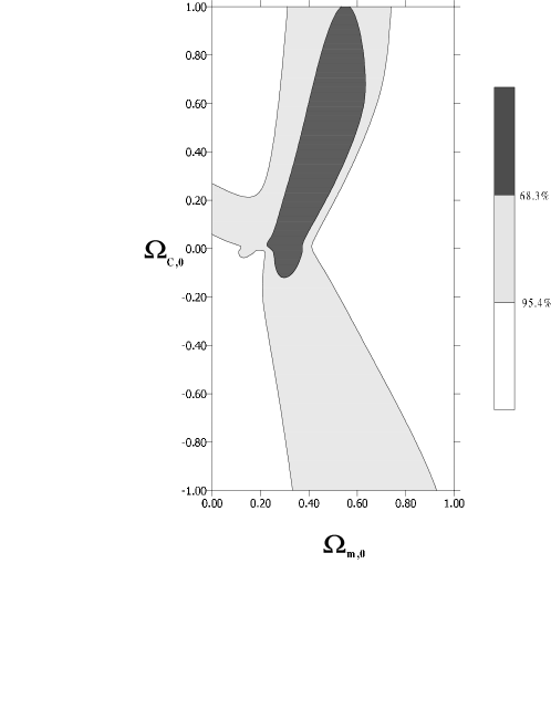
Figure 6: Confidence levels on the plane $(\Omega_{\mathrm{m},0},\Omega_{\mathrm{C},0})$ minimised over remaining model parameter. The figure shows of the preferred value of $\Omega_{\mathrm{m},0}$ and $\Omega_{\mathrm{C},0}$.

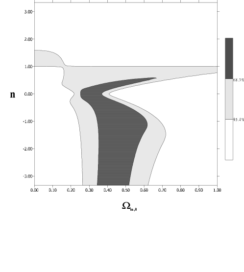
Figure 7: Confidence levels on the plane $(\Omega_{\mathrm{m},0},n)$ minimised over remaining model parameter. The figure shows of the preferred value of $\Omega_{\mathrm{m},0}$ and $n$.

Please note that both positive and negative values of $\Omega_{\text{C},0}$ are formally possible. It is the reason why we received on the Figs 4 and 5 bimodal distributions. Figs 6 and 7 explain this situation in more details. These figures present the confidence levels on the plane $(\Omega_{\text{m},0},\Omega_{\text{C},0})$ (Fig. 6) and $(\Omega_{\text{C},0},n)$ (Fig. 7) minimised over remaining model parameter.

Fig. 7 is more complicated than in the case of the model with $\Omega_{\Lambda}=0$ (see Fig. 4 in Ref. Godlowski04 where the maximum likelihood procedure suggests that $n$ should be negative and consequently $\Omega_{\text{m},0}$ is greater than $0.3$). Now we obtain also the possibility that $n>0$ and $\Omega_{\text{m},0}>0.3$ as a result of presence both $\Omega_{\text{C},0}$ and $\Omega_{\Lambda}$ terms.

The density distribution for model parameters for the model with fixed $\Omega_{\text{m},0}=0.3$ is presented on Figs 8-10. Those figures confirmed that in this case the model is close to $\Lambda$CDM model.

For the model with vanishing cosmological constant $\Omega_{\Lambda}=0$ the errors of the model parameters estimation is presented on Table 4. For this model, using the maximum likelihood method, we obtained with the sample K6 that $\Omega_{\text{m},0}=0.52^{+0.09}_{-0.09}$ and $n=-3.33^{+2.00}$ on the confidence level $68.3\%$. In turn, for sample K3 we obtained that $\Omega_{\text{m},0}=0.48^{+0.08}_{-0.13}$ and $n=-0.40^{+0.77}_{-1.24}$ on the confidence level $68.3\%$. With the new Riess et al. sample we obtain $\Omega_{\text{m},0}=0.51^{+0.04}_{-0.05}$ and $n=-1.60^{+0.74}_{-1.10}$ with the Silver sample, while with the Gold sample $\Omega_{\text{m},0}=0.51^{+0.04}_{-0.05}$ and $n=-1.23^{+0.73}_{-1.23}$. The best fit procedure also suggests that $n$ should be negative and consequently $\Omega_{\text{m},0}$ is greater than $0.3$.

One can see that that result obtained with maximum likelihood method, for $\Omega_{\text{m},0}$ and $\Omega_{\text{C},0}$ are similar for all samples, however with new Riess et al.’s sample errors in parameter estimation significantly decreased. Please note that with assumption that $\Lambda=0$ the model is equivalent to the Cardassian models. We confirmed our previous results Godlowski04 on the new Riess et al.’s sample. The observations favour the high density universe with $n$ negative. On the other hand, if we assume $\Omega_{\text{m},0}=0.3$ then $n\simeq 0$ which correspond to $\Lambda$CDM model, like for scaling multifluids model with non vanishing $\Lambda$.

For the model with $\Omega_{\text{m},0}=0.3$ we obtained for sample K6 $n=-0.13$ with $\sigma(n)=0.23$. In turn, for sample K3 we obtained $n=-0.20$, $\sigma(n)=0.17$. With the new Riess et al. sample we obtained $n=-0.07$ with $\sigma(n)=0.10$ for Silver sample, while $n=-0.03$, $\sigma(n)=0.10$ for Gold sample. On can see that result obtained with both samples are similar but with the Riess et al. sample errors in estimation of the parameters significantly decreased. These results mean that if we assume $\Omega_{\text{m},0}=0.3$ then $n\simeq 0$ which correspond to $\Lambda$CDM model.

In this way, it is crucial to determine which combination of parameters give the preferred fit to data. This is the statistical problem of model selection Liddle04 . The problem is usually the elimination of parameters which play insufficient role in improving the fit data available. Important role in this area plays especially the Akaike information criterion AIC Akaike74 . This criterion is defined as

$$AIC=-2\ln{\mathcal{L}}+2k$$ (43)

where $\mathcal{L}$ is the maximum likelihood and $k$ is the number of the parameter of the model. The best model is the model which minimises the AIC.

The Bayesian information criterion BIC introduced by Schwarz Schwarz:1978 is defined as:

$$\mathrm{BIC}=-2\ln{\mathcal{L}}+d\ln{N}$$ (44)

where $N$ is the number of data points used in the fit. While AIC tends to favour models with large number of parameters, the BIC the more strongly penalises them, so BIC provides the useful approximation to full evidence in the case of no prior on the set of model parameters Parkinson:2005 .

The effectiveness of using these criteria in the current cosmological applications has been recently demonstrated by Liddle Liddle04 Please note that both information criteria values have no absolute sense and only the relative values between different models are physically interesting. For the BIC a difference of $2$ is treated as a positive evidence ($6$ as a strong evidence) against the model with larger value of BIC Jeffreys:1961 ; Mukherjee:1998wp .

The AIC for the models under consideration is presented in the (Table 5) while for BIC in the (Table 6). The BIC information criterion do not show significant differences between scaling multifluid model with vanishing $\Lambda$ and $\Lambda$CDM model. The model which minimising AIC is scaling multifluids model with the vanishing cosmological constant (equivalent to the Cardassian model). It means that, from the statistical point of view, if we compare scaling multifluid models with vanishing and non-vanishing $\Lambda$, the extra term with $\Lambda$ does not improve significantly the quality of the fit.

Basing on AIC information criterion, it is clear that the scaling multifluid model with vanishing $\Lambda$ fits better to data then the $\Lambda$CDM model. However scaling multifluid model with vanishing $\Lambda$ indicate high density universe, with $\Omega_{m,0}\simeq 0.5$ which seems to be too high with comparison with present extragalactic data Peebles03 . Scaling multifluid model with non-vanishing $\Lambda$ allow density of the universe $\Omega_{m,0}$ close to 0.3 (Fig.7) while $\Lambda$CDM model predict $\Omega_{m,0}\simeq 0.3$. It clearly shows that more precise measurements of $\Omega_{m,0}$ from independent observations is necessary to final discriminate between the $\Lambda$CDM and scaling multifluid models.

VIII Conclusion

The Supernova Cosmology Project and the High–Z–Supernova Search reported of their observations of type Ia supernovae and suggest that the expansion of the Universe is still accelerating due to the presence of unknown form of matter called dark energy. For the accelerating Universe the equation of state parameter $w=\frac{p}{\rho}$ for dark must satisfy $w<-\frac{1}{3}$. The cosmological constant $\Lambda$ is arguable, but at the some time the simplest candidate for this dark energy, although it is well known, that predictions for its value are many orders of magnitude off from the observationally acceptable value. The introducing of $\Lambda=\Lambda(a)$ or quintessence is usually proposed as a possible solution to avoid the cosmological constant problem.

In presented paper the idea of derivation the form of equation of state from symmetries of self-similarity of the FRW dynamics is considered. We have shown that these symmetries enforce appropriate equation of state used commonly in cosmology. The property of homology is very important in astrophysics, when main sequence in the Hertzsprung–Russell diagram can be reconstructed from the invariants of homology transformations. Moreover from the Strömgren’s theorem, new solution of stellar structure equation can be obtained from the known ones through the homologous transformation. The new solutions describe new configurations with different masses, radius and chemical compositions (the so–called homologous stars). For recently obtained results see Stromgren37 ; Szydlowski04 where this problem is addressed in the context of brane cosmology. We pointed out that our Universe is also homological provided that it is filled by matter with the form of equation of state for noninteracting mixture of fluids $p=-\Lambda+C_{1}\rho(a)+C_{2}a^{\delta}$ and $\rho=\Lambda+\rho_{01}a^{-3(1+w)}+\rho_{02}a^{\delta}+\rho_{03}a^{-3}$. This form is commonly used in cosmological considerations. The key idea of this work is derivation this form of the equation of state from the first principles. It is proposed to derivate $p=p(\rho)$ from postulate of self-similarity of its dynamics. This property is well known to engineers who build ship models as a prototype of real ship. It is justified by the fact that Navier-Stoke’s equation are invariant against similarity symmetries.

As a result we obtain the commonly used form of equation of state for mixture of noninteracting, dust matter, dark energy (the cosmological constant) and cosmic time variation of cosmological constant parameterised by the scale factor. Therefore subliminal role of mathematics can also be seen in cosmology when we are looking for adequate form of equation of state for dark energy.

We showed that the model with scaling multifluids fits well the supernovae data. For simplicity of presentation we demonstrate this for the case $C_{1}=\rho_{01}=0$. Physically it means that the Universe is filled generally by dust matter, cosmological constant fluid and additional scaling fluid which comes from Cardassian modification of the FRW equation (or equivalently it it is scaling fluid describing phantom fields for example).

For the scaling multifluids model with $\Lambda\neq 0$, we found that $\Omega_{\text{m},0}\simeq 0.4$ with $n\simeq-1$ which correspond to (hyper) phantom model. If we assume $\Omega_{\text{m},0}=0.3$ from independent extragalactic estimation, then $\Omega_{\text{C},0}$ is small while value of $n$ close to zero is favoured and model becomes close to $\Lambda$CDM. With assumption that $\Lambda=0$ the model is equivalent to Cardassian models. We confirmed our previous results Godlowski04 on the new Riess sample. In particular the observations favour high density Universe with $n$ negative. Again, if we assume $\Omega_{\text{m},0}=0.3$ then $n\simeq 0$ which correspond to $\Lambda$CDM model.

¿From Fig. 1 can be seen the $m$-$z$ relation for our model and $\Lambda$CDM one. We observed that distant SNIa should be brighter (in our model) than in the $\Lambda$CDM model. What is interesting that the Hubble diagram for the model under consideration intersects the corresponding $\Lambda$CDM diagram. In such a way the supernovae on intermediate distant are fainter then expected in $\Lambda$CDM model. This predictions could be tested with the future supernovae data.

Our results demonstrate the existence of alternative model to $\Lambda$CDM model in explanation SNIa data. Therefore it should be interesting to compare both models from the point of view Akaike information criterion. Our result show that scaling multifluids model with vanishing $\Lambda$ significantly better fits data then $\Lambda$CDM model.

Moreover the cosmological model filled by scaling fluid makes a step toward solving the coincidence problem of the present value of dark matter and dark energy components Amendola00 .

To make the ultimate decision which model describes our Universe it is necessary to obtain the precise value of $\Omega_{m,0}$ from independent observations because $\Lambda$CDM model and scaling multifluid models predict different density of the Universe.

IX Acknowledgements

M.S. was supported by KBN grant 1 PO3D 003 26.

Table 1: Results of the statistical analysis of the model obtained both for the Knop et al. and Riess et al. samples from the best fit with minimum $\chi^{2}$ (denoted with BF) and from the likelihood method (denoted with L). The same analysis was repeated with fixed $\Omega_{\text{m},0}$.

sample	$\Omega_{\mathrm{m},0}$	$\Omega_{\mathrm{C},0}$	$n$	$\Omega_{\Lambda,0}$	$\mathcal{M}$	$\chi^{2}$	method
K6	0.64	0.58	-3.17	-0.22	-3.61	53.4	BF
	0.38	0.64	-2.10	0.72	-3.53	—	L
	0.05	0.03	2.60	0.92	-3.53	55.1	BF
	0.05	0.03	0.43	0.92	-3.51	—	L
	0.30	0.13	-3.33	0.57	-3.55	55.1	BF
	0.30	0.00	0.00	0.70	-3.52	—	L
K3	0.45	0.98	-0.47	-0.43	-3.49	60.3	BF
	0.27	0.01	0.00	0.75	-3.47	—	L
	0.05	0.05	1.97	0.90	-3.48	60.4	BF
	0.05	0.03	0.40	0.92	-3.46	—	L
	0.30	0.13	-2.23	0.57	-3.49	60.5	BF
	0.30	0.00	0.00	0.69	-3.46	—	L
Silver	0.44	0.32	-3.27	0.24	15.895	226.7	BF
	0.46	0.40	-1.10	0.12	15.915	—	L
	0.05	0.07	1.77	0.88	15.935	229.4	BF
	0.05	0.07	1.50	0.88	15.945	—	L
	0.30	0.10	-3.33	0.60	15.915	230.9	BF
	0.30	0.09	0.00	0.61	15.945	—	L
Gold	0.43	0.28	-3.33	0.29	15.905	172.1	BF
	0.44	0.34	-0.90	0.20	15.935	—	L
	0.05	0.10	1.57	0.85	15.945	174.0	BF
	0.05	0.09	1.30	0.86	15.945	—	L
	0.30	0.07	-3.33	0.63	15.925	175.2	BF
	0.30	0.00	0.00	0.70	15.945	—	L

Table 2: Results of the statistical analysis of the model with fixed $\Omega_{\Lambda,0}=0$ obtained both for the Knop et al. and Riess et al. samples from the best fit with minimum $\chi^{2}$ (denoted with BF) and from the likelihood method (denoted with $L$). The same analysis was repeated with fixed $\Omega_{\text{m},0}$.

sample	$\Omega_{\mathrm{m},0}$	$\Omega_{\mathrm{C},0}$	$n$	$\Omega_{\Lambda,0}$	$\mathcal{M}$	$\chi^{2}$	method
K6	0.54	0.46	-3.33	0.	-3.60	53.5	BF
	0.52	0.48	-3.33	0.	-3.55	—	L
	0.05	0.95	0.33	0.	-3.51	56.3	BF
	0.05	0.95	0.30	0.	-3.51	—	L
	0.30	0.70	-0.10	0.	-3.52	55.6	BF
	0.30	0.70	-0.13	0.	-3.53	—	L
K3	0.42	0.58	-0.77	0.	-3.49	60.3	BF
	0.48	0.52	-0.40	0.	-3.49	—	L
	0.05	0.95	0.30	0.	-3.46	61.5	BF
	0.05	0.95	0.30	0.	-3.46	—	L
	0.30	0.70	-0.13	0.	-3.47	60.6	BF
	0.30	0.70	-0.17	0.	-3.48	—	L
Silver	0.50	0.50	-1.73	0.	15.905	227.1	BF
	0.51	0.49	-1.60	0.	15.905	—	L
	0.05	0.95	0.40	0.	15.975	239.3	BF
	0.05	0.95	0.40	0.	15.965	—	L
	0.30	0.70	-0.07	0.	15.945	232.3	BF
	0.30	0.70	-0.07	0.	15.945	—	L
Gold	0.49	0.51	-1.37	0.	15.915	172.5	BF
	0.51	0.49	-1.23	0.	15.915	—	L
	0.05	0.95	0.43	0.	15.975	180.8	BF
	0.05	0.95	0.43	0.	15.975	—	L
	0.30	0.70	-0.03	0.	15.945	175.9	BF
	0.30	0.70	-0.03	0.	15.945	—	L

Table 3: Model parameter values obtained from the minimisation procedure carried out with the Knop et al. and Riess et al. samples.

sample	$\Omega_{\mathrm{m},0}$	$\Omega_{\mathrm{C},0}$	$\Omega_{\Lambda,0}$	$n$
K6	$0.38^{+0.32}_{-0.18}$	$0.64^{+0.36}_{-0.48}$	$0.72^{+0.30}_{-0.32}$	$-2.10^{+1.63}_{-1.23}$
	$0.05$	$0.03^{+0.38}_{-0.76}$	$0.92^{+0.76}_{-0.38}$	$0.43^{+0.97}_{-2.00}$
	$0.3$	$0.00^{+0.38}_{-0.23}$	$0.70^{+0.23}_{-0.38}$	$0.00^{+0.58}_{-1.70}$
K3	$0.27^{+0.20}_{-0.13}$	$0.01^{+0.63}_{-0.38}$	$0.75^{+0.38}_{-0.70}$	$0.00^{+0.93}_{-1.56}$
	$0.05$	$0.03^{+0.38}_{-0.76}$	$0.92^{+0.76}_{-0.38}$	$0.40^{+0.96}_{-1.90}$
	$0.3$	$0.00^{+0.38}_{-0.20}$	$0.69^{+0.21}_{-0.37}$	$0.00^{+0.50}_{-1.60}$
Silver	$0.46^{+0.10}_{-0.08}$	$0.40^{+0.34}_{-0.22}$	$0.12^{+0.30}_{-0.44}$	$-1.10^{+0.50}_{-1.75}$
	$0.05$	$0.07^{+0.09}_{-0.04}$	$0.88^{+0.04}_{-0.09}$	$1.50^{+0.40}_{-0.47}$
	$0.3$	$0.09^{+0.17}_{-0.20}$	$0.61^{+0.20}_{-0.17}$	$0.00^{+0.36}_{-1.20}$
Gold	$0.44^{+0.11}_{-0.11}$	$0.34^{+0.39}_{-0.33}$	$0.20^{+0.55}_{-0.47}$	$-0.90^{+0.60}_{-1.90}$
	$0.05$	$0.09^{+0.15}_{-0.05}$	$0.86^{+0.05}_{-0.15}$	$1.30^{+0.43}_{-0.47}$
	$0.3$	$0.00^{+0.26}_{-0.17}$	$0.70^{+0.17}_{-0.26}$	$0.00^{+0.50}_{-1.60}$

Table 4: Model parameter values obtained from the minimisation procedure carried out on the Knop and Riess samples. Model with fixed $\Omega_{\Lambda,0}=0$.

sample	$\Omega_{\mathrm{m},0}$	$\Omega_{\mathrm{C},0}$	$\Omega_{\Lambda,0}$	$n$
K6	$0.52^{+0.09}_{-0.09}$	$0.48^{+0.09}_{-0.09}$	$0.$	$-3.33^{+2.00}_{-0.00}$
K3	$0.48^{+0.08}_{-0.13}$	$0.52^{+0.13}_{-0.08}$	$0.$	$-0.40^{+0.77}_{-1.24}$
Silver	$0.51^{+0.04}_{-0.05}$	$0.49^{+0.05}_{-0.04}$	$0.$	$-1.60^{+0.74}_{-1.10}$
Gold	$0.51^{+0.04}_{-0.05}$	$0.49^{+0.05}_{-0.04}$	$0.$	$-1.23^{+0.73}_{-1.23}$

Table 5: The Akaike information criterion (AIC) for models: $\Lambda$CDM model ($\Lambda$CDM), Cardassian and Scaling Multifluids.

sample	$\Lambda$CDM	Cardassian	Scaling Multifluids
K6	59.8	59.5	61.4
K3	64.3	66.3	68.3
Silver	236.6	233.1	234.7
Gold	179.9	178.5	180.1

Table 6: The Bayesian information criterion (BIC) for models: $\Lambda$CDM model ($\Lambda$CDM), Cardassian and Scaling Multifluids.

sample	$\Lambda$CDM	Cardassian	Scaling Multifluids
K6	63.8	65.5	69.4
K3	68.3	72.3	76.3
Silver	243.0	242.8	247.6
Gold	186.0	186.7	196.3

Figure 1: Riess Gold sample, M=15.935 Residuals (in mag) between the Einstein-de Sitter model and four cases: the Einstein-de Sitter itself (zero line), the $\Lambda$CDM flat model (upper curve), the best-fitted model (upper-middle curve), $\Omega_{\mathrm{m},0}=0.43$, $\Omega_{C,0}=0.28$, $\Omega_{\Lambda,0}=0.29$, $n=-3.33$, and the best-fitted $\Lambda=0$ model (lower-middle curve) $\Omega_{\mathrm{m},0}=0.49$, $\Omega_{C,0}=0.51$, $n=-1.37$.

Figure 2: The density distribution for $\Omega_{\mathrm{m},0}$. We obtain that $\Omega_{\mathrm{m},0}=0.44^{+0.11}_{-0.11}$ on the confidence level $68.3\%$ (the inner dash lines). Additionally the confidence level $95.4\%$ is marked (the outer dash lines).

Figure 3: The density distribution for $\Omega_{C,0}$. We obtain that $\Omega_{C,0}=0.34^{+0.39}_{-0.33}$ on the confidence level $68.3\%$ (the inner dash lines). Both positive and negative values of $\Omega_{C,0}$ are formally possible.

Figure 4: The density distribution for $n$. We obtain that $n=-0.90^{+0.60}_{-1.90}$ on the confidence level $68.3\%$ (the inner dash lines). Additionally the confidence level $95.4\%$ is marked (the outer dash lines). Both positive and negative values of $n$ are formally possible.

Figure 5: The density distribution for $\Omega_{\Lambda,0}$. We obtain that $\Omega_{\Lambda,0}=0.20^{+0.55}_{-0.47}$ on the confidence level $68.3\%$ (the inner dash lines). Additionally the confidence level $95.4\%$ is marked (the outer dash lines).

Figure 8: The density distribution for $\Omega_{C,0}$ for the model with $\Omega_{\mathrm{m},0}$=0.3. We obtain that $\Omega_{C,0}=0.00^{+0.26}_{-0.17}$ on the confidence level $68.3\%$ (the inner dash lines). Additionally the confidence level $95.4\%$ is marked (the outer dash lines). Both positive and negative values of $\Omega_{C,0}$ are formally possible.

Figure 9: The density distribution for $n$ for the model with $\Omega_{\mathrm{m},0}$=0.3. We obtain that $n=0.00^{+0.50}_{-1.60}$ on the confidence level $68.3\%$ (the inner dash lines). Additionally the confidence level $95.4\%$ is marked (the outer dash lines).

Figure 10: The density distribution for $\Omega_{\Lambda,0}$ for the model with $\Omega_{\mathrm{m},0}$=0.3. We obtain that $\Omega_{\Lambda,0}=0.70^{+0.17}_{-0.26}$ on the confidence level $68.3\%$ (the inner dash lines). Additionally the confidence level $95.4\%$ is marked (the outer dash lines).

References

- (1) Sachs R. K., Wu H. Gen. Relat. for Math. 1977
- (2) Szydlowski M., Heller M., Acta Phys. Pol B14 571 1983
- (3) McCrea, W. H., Proc. R.Soc. London A206, 569, 1951
- (4) Peebles P. J. E., Ratra B., Rev. Mod. Phys.75, 559, 2003
- (5) Perlmutter S., Aldering G., Goldhaber G., et al., Astrophys. J 517, 565, 1999
- (6) Riess A., et al., Astron. J 116, 1009, 1998
- (7) Stephani H., Differential equation - Their solution using symmetries, eds MacCallum M., Cambridge University Press, Cambridge, 1989;
- (8) Aguirregabiria J. M., et al. Phys. Rev. D67, 083518, 2003
- (9) Chimento L. P., Phys. Rev. D65, 0633517, 2002
- (10) Belinchon J. A., Davila, Class. Quantum Grav. 17, 3183, 2000
- (11) Belinchon J. A., Harko T., Mak M.K. Class. Quantum Grav. 19, 3003, 2002
- (12) Arnold V. Chaptiers supplementataires de la theorie des équations differentiales ordinaries, Mir, Moscow, 1980.
- (13) Collins C. B. Gen. Relativ. Grav. 8, 717, 1977
- (14) Collins C. B. J. Math. Phys. 18, 1374, 1977
- (15) van den Hoogen R.J., Coley A.A., Wands D. Class. Quantum Grav. 16, 1843, 1999
- (16) Carr B.J., Coley A.A. Class. Quantum Grav. 16, R31, 1999
- (17) Maeda H., Harada T. gr-qc/0405113
- (18) Carr B.J., unpublished 1993
- (19) Harada T., Maeda H. Phys. Rev. D63, 084022, 2001
- (20) Choptuik M.W. Phys. Rev. Lett. 70, 9, 1993
- (21) Guo Z.K., Zhang Y.Z. astro-ph/0411524
- (22) Tsujikawa S., Sami M., hep-th/0409212
- (23) Gumjudpai B., Naskar T., Sami M., Tsujikawa S. hep-th/0502191
- (24) Amendola L., Tocchini- Valentini D. astro-ph/0011243
- (25) Sahni V. Class. Quantum Grav. 19 3435, 2002
- (26) Amendola L., astro-ph/9904120
- (27) Amendola L., Gasparini M., Piazza F. astro-ph/0407573
- (28) Majerrotto E., Sapone D., Amendola L. astro-ph/0410543
- (29) Ellis G.F.R., Buchert T., gr-qc/0506106
- (30) Harko T., Mak M. K. Phys. Rev. D69, 064020, 2004
- (31) Copeland E.J., Liddle A.R., Wands D. Phys. Rev. D57, 4686, 1998
- (32) Falle S. Mon. Not. R. Astr. Soc. 250, 581 1991),
- (33) Ibragimov N. K. Transformations in Mathematical Physics Moscow 1983
- (34) Hydon P. E. Symmetry Methods for Differential Equation, Cambridge University Press, Cambridge, 1999
- (35) Biesiada M., Szydlowski M., Szczesny J. Acta Cosmologica XVI, 115, 1989
- (36) Lue A., Starkman G. D., Phys. Rev. Lett. 92, 131102, 2004
- (37) Jafarizadeh M. A., et al. Phys. Rev. D60, 063514, 1999
- (38) Silveira V., Waga I. Phys. Rev. D56, 4625, 1997
- (39) Alam U., Sahni V., Starobinsky A. A. JCAP 04, 002, 2003
- (40) Gorini V., Kamenschik A., Morchella U., Pasquier V., gr-qc/0403062, 2004
- (41) Godlowski W., Szydlowski M., Gen. Relat. Grav. 35, 2171, 2003
- (42) Godlowski W., Szydlowski M., Krawiec A., Astrophys. J 605, 599, 2004
- (43) Godlowski W., Szydlowski M., Gen. Relat. Grav. 36, 767, 2004
- (44) Dabrowski M.P., Godlowski W., Szydlowski M. Int. J. Mod. Phys. D13, 1669, 2004
- (45) Godlowski W., Stelmach J., Szydlowski M. Class. Quantum Grav., 21, 3953, 2004
- (46) Biesiada M., Godlowski W., Szydlowski M., Astrophys. J. 622 28, 2005
- (47) Molina-Paris C., Visser M. Phys. Lett B 455 90 1999
- (48) Tippett B.K., Lake K. gr-qc/0409088
- (49) Szydlowski M., Godlowski W., Krawiec A., Golbiak J. Phys Rev D72 063504, 2005
- (50) Boyowald M. Phys. Rev Lett. 86, 5227, 2001
- (51) Boyowald M. Phys. Rev Lett. 89, 261301, 2002
- (52) Nojiri S., Odintsov S.D. Phys. Lett. B595, 1, 2004
- (53) Elizalde E., Nojiri S., Odintsov S.D. Phys. Rev. D70, 043539, 2004
- (54) Nojiri S., Odintsov S.D. Phys. Rev. D70, 103522, 2004
- (55) Tolman R.C, Relativity Thermodynamics and Cosmology Oxford University Press, Oxford, 1934
- (56) Robertson H.P. Rev. Mod. Phys.5, 62 1933
- (57) Einstein A. Berl. Ber. 235 1931
- (58) Tolman R.C. Phys. Rev. 38 1758 1931
- (59) Steinhard P.J., Turok N. Nucl. Phys. Proc. Suppl. 124 38 2003
- (60) Shtanov Y, Sahni V. Class. Quantum Grav. 19, L101 2002
- (61) Coule D.H., Class. Quantum Grav. 22, R125 2005
- (62) Salim J. M., Perez Bergliaffa S. E., Souza ., Class. Quantum Grav. 22 975 2005
- (63) Pinto Neto ., Int. J. Mod. Phys. D13, 1419 2004
- (64) Barrow J. D., Kimberly D., Magueijo J., Class. Quantum Grav. 21 4289 2004
- (65) Bennett C. L. et al. Astrophys. J. Suppl. 148 1, 2003
- (66) Barris B. J. et al.Astrophys. J 602, 571, 2004.
- (67) Choudhury T.R., Padmanabhan T. Astron. Astrophys. 429, 807, 2005
- (68) Knop R. A. et al. Astrophys.J 598, 102, 2003
- (69) Riess A., Nugent P.E., Gilliland R.L., et al., Astrophys. J. 560, 49, 2001
- (70) Riess A. G. et al. Astrophys. J. 607, 665, 2004
- (71) Tonry J. L., et al., Astrophys. J. 594, 1, 2003
- (72) Williams B. F. et al., 2003 astro-ph/0310432
- (73) Freese K., Lewis, M., Phys. Lett. B 540, 1, 2002
- (74) Zhu Z.-H., Fujimoto M.-K., Astrophys. J. 585, 52, 2003
- (75) Sen S., Sen A. A. Astrophys. J. 588, 1, 2003
- (76) Liddle A.R., astro-ph/0401198 2004
- (77) Akaike H., IEEE Trans. Auto Control 19, 716, 1974
- (78) Schwarz G., Annals of Statistics 5 461, 1978
- (79) Parkinson D., Tsujikawa S., Basset B., Amendola L. Phys Rev D71 063524, 2005
- (80) Jeffreys H., Theory of Probability, 3rd Edition, Oxford University Press, Oxford, 1961
- (81) Mukherjee S., Feigelson E. D., Babu G. J., Murtagh F., Fraley C., Raftery A., Astrophys. J. 508 314, 1998
- (82) Strömgren B. Exapt. Ery. Naturw. 16 465, 1937
- (83) Szydlowski M., Maciejewski A. J. Phys. bf A37, 1, 2004