Precise Reddening and Metallicity of NGC6752 from FLAMES spectra

Accurate reddenings for Globular Clusters could be obtained by comparing the colour-temperature obtained using temperatures from reddening-free indicator ($H\alpha$), with that given by standard colour-temperature calibrations. The main difficulty in such derivations is the large errors in temperatures for individual stars due to uncertainties on the removal of instrumental signature for each individual star. The large multiplexing opportunity offered by FLAMES at VLT2 allowed us to obtain spectra centred on $H\alpha$ at a resolution of R=6000 and $5<S/N<50$ for 120 stars near the turn-off of NGC6752 with GIRAFFE from a single 1300 seconds exposure. This set of spectra was used to derive effective temperatures from fittings of $H\alpha$ profiles with typical errors of about $\pm 200$ K and reddening estimates with individual errors of 0.05 mag. Averaging all individual reddenings, a high precision reddening estimate has been obtained for the cluster: $E(B-V)=0.046\pm 0.005$. The same exposure provided UVES spectra of seven stars near the red giant branch bump at a resolution of 40,000, and $20<S/N<40$. These spectra, combined with temperatures from colours (corrected for our high precision reddening value) provided Fe abundances with internal errors of 0.026 dex, and with average metallicity [Fe/H]=$-1.48\pm 0.01\pm 0.06$ dex (random + systematic). Abundances were obtained for several other elements, allowing e.g. an accurate estimate of the ratio between the $\alpha-$elements and Fe ([$\alpha$/Fe]=$+0.27\pm 0.01$). The O-Na anticorrelation is evident from our UVES data, in agreement with past results.
This analysis shows the power of FLAMES for analysis of globular clusters: the accurate reddenings and metal abundances obtained by a procedure like that described here, combined with distance determinations from cluster dynamics or main sequence fitting, and high quality colour-magnitude diagrams, could allow derivation of ages with errors below 1 Gyr for individual globular clusters.

1 INTRODUCTION

Accurate estimates of the absolute ages of (the oldest) Globular Clusters (GCs), coupled with determinations of the Hubble constants $H_{0}$ from the spectrum of fluctuations of the microwave background determined from the WMAP experiment (Spergel et al. 2003), or from the HST Key Project (Freedman et al. 2001), may provide a stringent lower limit to the age of the Universe and constrains the exponent $w$ of the equation of state of the dark energy (Jimenez et al. 2003), independently of type Ia SN observations (see e.g. Gratton et al. 2003a).

Furthermore, within the framework of a standard $\Lambda$CDM model, where the age of the Universe is accurately fixed at $13.7\pm 0.2$ Gyr by the WMAP results (Spergel et al. 2003), the age of GCs can be used to constrain the epoch of formation of the Galaxy, linking the local Universe to the distant one (see Carretta et al. 2000; and Gratton et al. 2003a).

Relative ages are fundamental to describe the early history of our Galaxy. In this framework it should be noted that galactic GCs divide into two main groups: halo and thick disk (or bulge) GCs (Zinn 1985). The differential ages method suggests that these two groups might have ages different by about 2 Gyr (Rosenberg et al. 1999); this result seems supported by absolute ages (Gratton et al. 2003a). This has implications for both cosmology (where only the oldest GCs are of interest) and galactic evolution. Observations of GC systems in other galaxies suggest a link between GC formation and strong dynamical interactions (Peebles & Dicke 1968; Schweizer & Seitzer 1993). The oldest group of GCs might then be related to the very early phases of the galactic collapse, while the second one may instead trace a later accretion event (see Freeman & Bland-Hawthorn, 2002), possibly related to the end of the thick disk phase indicated by chemistry (Gratton et al. 1996, Gratton et al. 2000; Fuhrmann 1998).

An important goal is then to derive absolute ages with internal errors of $\pm 1$ Gyr for an ample sample of GCs. Ages for GCs with such small errors may be derived only using the luminosity of the turn-off (TO): this on turn requires accurate distances, with errors $<5\%$. In perspective, most accurate and robust distances (error $<2$%) for a few GCs will be obtained using geometrical methods (Piotto et al 2004). At present, distances with errors of 3-5% can be obtained for a larger sample of GCs using the Main Sequence Fitting Method (MSFM), exploiting local subdwarfs as standard candles (see Gratton et al. 1997; Pont et al. 1998; Carretta et al. 2000; Gratton et al. 2003a). Main sources of errors in MSFM are possible systematic differences in reddenings and metallicities between field and GC stars (accurate initial He abundances in GCs have been determined by Cassisi et al. 2003; see also Salaris et al. 2004). Both of them can be reduced to within the required accuracy if a reddening-free temperature indicator is used for both field and GC stars of similar evolutionary phases: the analysis of the results of the ESO LP 165.L-0263 (Gratton et al. 2003a) relative to three GCs (NGC6397, NGC6752 and 47 Tuc) spanning almost the total metallicity range of galactic GCs showed that this approach may provide reddenings accurate to $\Delta(B-V)=\pm 0.005$ mag, metallicities accurate to $\pm 0.04$ dex, distances accurate to 4%, and ages with errors of about $\pm 1$ Gyr. Also geometrical distances (which determines the true distance modulus toward a cluster) will take advantage from accurate reddening and metallicity determinations, since apparent distance moduli are required to derive ages.

Note that here we are only interested in relative reddening and metallicity determinations: the adopted scale may be tied to that of field stars exploiting the clusters observed within the LP 165.L-0263 (47 Tuc, NGC6397, and NGC6752: Gratton et al. 2003a). The same temperature indicator may be adopted (H$\alpha$ profile).

In this paper we describe a pilot program on NGC6752 which exploits the multiplexing capabilities of FLAMES, the VLT multifibre facility (Pasquini et al. 2002). The large number of spectra that could be obtained using GIRAFFE allowed a proper reduction of the major source of errors in temperatures derived from H$\alpha$: flat fielding. On the other side, low resolution and S/N were not too critical in such observations, allowing to use faint turn-off stars. The simultaneous acquisition of spectra of a few red giants with UVES allowed additionally an accurate determination of the chemical composition. For this purpose we preferred to use relatively warm stars, for which the analysis is expected to be robust. The success of this procedure suggests the usefulness of an extensive program on other globular clusters. Ages within $\pm 1$ Gyr are now fully within reach for a substantial sample of them in both Zinn’s groups.

Table 1: Summary of observations

Date	24/06/2004
Time (UT Start)	09:49:51
Exposure Time (sec)	1300
Airmass (Mean)	1.803
Seeing FWHM (arcsec)	0.62

2 OBSERVATIONS

Data used in this paper are based on a single 1300 seconds exposure obtained on June 24th, 2004, with FLAMES at Kueyen (=VLT2) used in service mode. The observations were obtained at a rather large airmass (about 1.8) and in very good seeing conditions (FWHM=0$\aas@@fstack{\prime\prime}$62 at zenith and 5000 Å) (see also Table 1).

120 fibres feeding the GIRAFFE spectrograph were centred on stars slightly brighter than the turn-off of NGC6752, in the magnitude range $16.7<V<17.2$. Stars were carefully selected from high quality photometric $UBV$ observations obtained with the Wide-Field Imager (WFI) at the 2.2 m ESO-MPI telescope (total field of view of $34\times 33$ arcmin²). For a detailed representation of the data reduction and calibration of this data set we refer the reader to Momany et al. (2004).

The astrometric calibration of NGC6752 reference images employed over 7000 stars from the GSC2.2 catalogue (Loomis et al. 2004), using the IRAF MSCRED package. The internal accuracy of the astrometry has been estimated to be about 0.15 arcsec, well within the FLAMES requirements (0.2 arcsec). To further confirm the fulfilment of the requirements, we matched our astrometrically calibrated NGC6752 catalogue with that of UCAC2 (Zacharias et al. 2004) and estimated the positional residuals for 550 stars in common. The residuals show a Gaussian distribution with an r.m.s. of $\simeq$0.05 arcsec in both coordinates.

Only uncrowded stars were considered, that is stars not showing any companion brighter than $V_{\rm target}+2$ mag within 2.5 arcsec, or brighter than $V_{\rm target}-2$ mag within 10 arcsec. The targets were selected to lie close to the cluster mean loci in the colour-magnitude diagram. A posteriori, radial velocities confirmed membership of all but two of the observed stars. Eight fibres were additionally used to monitor sky background; they were pointed toward carefully selected empty sky regions.

The GIRAFFE spectrograph was used with the LR06 grating; the spectra cover the wavelength range 6400-7100 Å at a resolution of about $R\sim 6000$. Pixel-to-pixel S/N of the spectra (measured from the scatter of individual spectral points in the wavelength range 6660-6670 Å) ranged from 5 to 50, with typical values around 20. The S/N values were generally lower for stars in the outer regions of the cluster, most likely because these stars were not well centred on the fibre heads. This can be attributed to the effects of differential refraction at the rather large airmass of observation.

The average of the eight sky spectra were used to subtract telluric emissions (in particular, emission in H$\alpha$) from GIRAFFE spectra. Appropriate scaling factors were evaluated to take into account the transmission of individual fibres.

Seven fibres feeding the UVES spectrograph were centred on stars close to the RGB bump ($13.2<V<14.2$), while one was dedicated to the sky. The spectra cover the wavelength range 4700-6900 Å, and have $20<S/N<40$.

The two sets of spectra were reduced using the dedicated FLAMES pipelines (BLDRS Python software 0.5.3 version for the GIRAFFE spectra; uves/2.1.1 version for UVES spectra). We found that this UVES pipeline does not accurately subtract the background between orders in the green-yellow part of the spectra. Only a few lines measured on these portions of the spectra were considered in the present analysis.

3 REDDENING ESTIMATES FROM GIRAFFE SPECTRA

3.1 Fluxes

The following procedure was used to derive accurate temperatures from the H$\alpha$ profile. First, instrumental fluxes within 10 narrow bands of 5 Å width in the region including $H\alpha$ were measured on the GIRAFFE spectra by integrating the observed spectra, after shifting them in wavelength for the geocentric radial velocity of each star. Cosmic ray hits were removed before evaluating the fluxes. The list of the bands used is given in Table 2.

Table 2: Definition of the bands used to derive T_eff’s

Band	Start	End
	(Å)	(Å)
1	6537.8	6542.8
2	6542.8	6547.8
3	6547.8	6552.8
4	6552.8	6557.8
5	6557.8	6562.8
6	6562.8	6567.8
7	6567.8	6572.8
8	6572.8	6577.8
9	6577.8	6582.8
10	6582.8	6587.8

The fluxes measured in each band were then normalized to a pseudocontinuum given by a straight line connecting the average of the first two bands with the average of the two last bands. The normalized fluxes for all the stars observed with GIRAFFE are given in Table 3 (available only in electronic form). The second column of this Table gives also the $S/N$ ratio for each spectrum, computed from the spectral region 6660-6670 Å, where there is no significant feature.

Since the $H\alpha$ profiles are expected to be fairly symmetric and since bands are defined symmetrically with respect to the line center, errors in these normalized fluxes can be obtained by comparing fluxes measured on the blue and red side of the $H\alpha$. Eliminating a few outliers, the comparisons are as follows:

$$5-6=-0.008\pm 0.002,\leavevmode\nobreak\ \leavevmode\nobreak\ \leavevmode\nobreak\ \leavevmode\nobreak\ {\rm r.m.s.}=0.019,\leavevmode\nobreak\ \leavevmode\nobreak\ \leavevmode\nobreak\ {\rm 112\leavevmode\nobreak\ stars}$$ (1)

and:

$$4-7=-0.013\pm 0.002,\leavevmode\nobreak\ \leavevmode\nobreak\ \leavevmode\nobreak\ \leavevmode\nobreak\ {\rm r.m.s.}=0.020,\leavevmode\nobreak\ \leavevmode\nobreak\ \leavevmode\nobreak\ {\rm 114\leavevmode\nobreak\ stars}$$ (2)

for bands 5-6 and 4-7. From these comparison, we expect a typical error in the average of $<5,6>$ bands of $\pm 0.0095$, corresponding to an internal error in T_eff’s of $\pm 110$ K (see next Section).

This error agrees with expectations based on the $S/N$ of the spectra.

Individual heliocentric radial velocities measured by the FLAMES pipeline are presented in the third column of Table  3. In a few cases (7 stars out of 120), these measures of the radial velocities by the automatic routine in the pipeline were obviously wrong, perhaps due to the strong telluric signal present in this wavelength range. Radial velocities for these stars were measured by fitting H$\alpha$, and zeroing the radial velocity on the telluric bands consistently with the other stars. All but one (29049) of the stars appear to be members of the cluster on the basis of radial velocity; the velocity for star 39462 is discrepant too, but this spectrum has very low S/N and we suspend judgement about it. However we excluded these two stars from our estimates of reddening of NGC6752. The mean radial velocity is $-32.0\pm 0.6$ km s^-1, with an r.m.s. scatter of individual values of 6.0 km s^-1 (118 stars), with no obvious correlation of the spread with S/N, nor distance from the cluster centre.

The average value of the radial velocity agrees very well with those estimated by Webbink (1988: $-32.2\pm 3.2$ km s^-1) and Dubath et al. (1997: $-32.0\pm 1.6$ km s^-1), while it is slightly larger than that given by Rutledge et al. (1997: $-27.4\pm 2.7$ km s^-1). For comparison, the seven stars observed with UVES provided a slightly lower average velocity ($-23.8\pm 2.1$ km s^-1, see Table 6).

Errors in the GIRAFFE radial velocities should be roughly 5-6 km s^-1, as given by the FLAMES pipeline. For comparison, the radial velocity error is expected to be roughly $\sigma(RV)\sim 33/(S/N)$ km s^-1 when using the formula by Landman et al. (1982) and assuming that all radial velocity signal is given by H$\alpha$ alone: for the typical $S/N$ of the program spectra, errors are then expected in the range 0.7-6 km s^-1. Given these large uncertainties on the errors attached to these radial velocities, they are of little use in estimating the internal velocity dispersion in NGC 6752.

Table 3: S/N ratios, heliocentric radial velocities and normalized fluxes for the target stars (Table to appear only in electronic form)

Star	$S/N$	$V_{r}$	3	4	5	6	7	8	$<5,6>$
		km s-1
1538	18	$-$34.0	0.008	0.042	0.273	0.291	0.073	0.008	0.282
1895	35	$-$35.6	0.021	0.043	0.217	0.242	0.039	0.029	0.229
2119	24	$-$35.4	0.015	0.047	0.218	0.253	0.053	0.024	0.236
2250	30	$-$28.8	0.024	0.069	0.243	0.251	0.061	0.012	0.247
2374	36	$-$42.2	0.021	0.038	0.293	0.167	0.033	0.010	0.230
2484	28	$-$33.1	0.020	0.031	0.216	0.240	0.032	0.009	0.228
2486	29	$-$31.4	0.005	0.023	0.207	0.224	0.035	0.008	0.215
2533	35	$-$28.3	0.010	0.030	0.222	0.244	0.030	0.019	0.233
2541	18	$-$27.9	0.027	0.070	0.265	0.286	0.076	0.013	0.276
2594	30	$-$30.6	0.003	0.035	0.217	0.231	0.044	0.013	0.224
2661	31	$-$31.4	0.008	0.030	0.210	0.199	0.036	0.018	0.204
2700	25	$-$42.8	0.009	0.037	0.285	0.163	0.022	-0.001	0.224
2750	27	$-$29.3	0.014	0.040	0.251	0.241	0.028	0.019	0.246
4606	11	$-$39.7	0.025	0.017	0.212	0.239	0.087	0.033	0.225
4693	27	$-$34.9	0.036	0.045	0.278	0.185	0.036	0.026	0.231
4905	27	$-$21.7	0.015	0.034	0.234	0.197	0.042	0.017	0.215
5540	18	$-$21.0	0.023	0.042	0.250	0.263	0.078	0.038	0.257
6057	26	$-$23.1	0.023	0.032	0.226	0.242	0.033	0.016	0.234
6439	27	$-$27.9	0.026	0.036	0.221	0.242	0.039	0.013	0.232
8265	16	$-$38.9	0.018	0.062	0.291	0.310	0.091	0.037	0.301
12600	29	$-$28.7	0.016	0.048	0.249	0.247	0.059	0.022	0.248
20454	33	$-$30.7	0.023	0.050	0.277	0.165	0.050	0.026	0.221
21163	33	$-$37.5	0.010	0.031	0.211	0.237	0.047	0.016	0.224
23507	23	$-$25.6	0.015	0.049	0.230	0.254	0.042	0.023	0.242
23697	27	$-$38.1	0.021	0.054	0.247	0.247	0.054	0.024	0.247
24300	33	$-$34.9	0.029	0.048	0.223	0.250	0.054	0.007	0.236
25443	31	$-$23.2	0.031	0.041	0.233	0.240	0.069	0.043	0.237
25518	54	$-$18.8	0.015	0.036	0.266	0.227	0.031	0.005	0.247
26038	29	$-$31.2	0.024	0.054	0.305	0.168	0.056	0.020	0.236
26672	25	$-$43.8	0.007	0.031	0.188	0.290	0.039	0.004	0.239
27210	30	$-$37.9	0.012	0.081	0.239	0.248	0.057	0.019	0.244
27611	26	$-$22.3	0.019	0.035	0.223	0.228	0.062	0.017	0.226
28023	34	$-$38.0	0.017	0.064	0.264	0.274	0.078	0.028	0.269
28047	40	$-$35.3	0.015	0.025	0.210	0.226	0.027	0.016	0.218
28440	28	$-$38.2	0.001	0.041	0.219	0.240	0.040	0.018	0.230
28598	36	$-$33.5	0.015	0.048	0.254	0.280	0.053	-0.014	0.267
29049	39	20.8	0.024	0.056	0.248	0.230	0.063	0.026	0.239
29206	35	$-$33.5	0.007	0.035	0.226	0.244	0.051	0.018	0.235
29380	27	$-$38.8	0.006	0.036	0.222	0.246	0.042	0.017	0.234
29767	22	$-$29.8	0.020	0.050	0.231	0.235	0.060	0.019	0.233
29778	29	$-$40.0	0.016	0.032	0.210	0.226	0.042	0.027	0.218
29827	32	$-$28.1	0.004	0.033	0.210	0.251	0.026	0.032	0.230
29986	20	$-$31.6	0.017	0.079	0.276	0.292	0.075	0.016	0.284
30188	18	$-$34.5	0.015	0.059	0.259	0.274	0.081	-0.003	0.266
30275	30	$-$20.9	0.019	0.067	0.279	0.218	0.066	0.020	0.249
30584	22	$-$33.0	0.036	0.049	0.232	0.236	0.053	0.030	0.234
30616	35	$-$33.2	0.004	0.023	0.215	0.221	0.048	0.036	0.218
30716	31	$-$31.6	0.028	0.057	0.242	0.262	0.061	0.025	0.252
30733	44	$-$23.2	0.032	0.042	0.263	0.241	0.075	0.048	0.252
30852	25	$-$44.9	0.005	0.057	0.250	0.276	0.080	0.054	0.263
30991	31	$-$29.4	0.033	0.053	0.220	0.251	0.050	0.014	0.235
31194	21	$-$26.5	0.041	0.041	0.259	0.263	0.058	0.046	0.261
31370	25	$-$33.6	0.014	0.034	0.266	0.281	0.051	0.015	0.273
31407	34	$-$29.0	0.025	0.029	0.210	0.211	0.039	0.031	0.210
31412	19	$-$27.6	0.032	0.042	0.255	0.241	0.075	0.048	0.248
31430	21	$-$30.1	0.035	0.062	0.249	0.240	0.072	0.019	0.245
31589	13	$-$28.5	0.040	0.008	0.271	0.280	0.085	0.006	0.276
31620	16	$-$38.1	0.036	0.058	0.243	0.267	0.072	0.023	0.255
31711	31	$-$33.4	0.008	0.037	0.231	0.232	0.044	0.017	0.231
31757	17	$-$36.6	0.043	0.059	0.284	0.285	0.061	0.038	0.284

Table 3: Normalized Fluxes (cont. in electronic form)

Star	$S/N$	$V_{r}$	3	4	5	6	7	8	$<5,6>$
		km s-1
31771	30	$-$36.2	0.008	0.042	0.213	0.220	0.062	0.022	0.216
31773	21	$-$20.2	0.022	0.040	0.237	0.238	0.045	0.001	0.237
31921	13	$-$29.8	0.015	-0.006	0.236	0.214	-0.025	-0.040	0.225
31945	21	$-$38.1	0.056	0.030	0.212	0.240	0.065	0.028	0.226
32027	21	$-$39.9	0.020	0.028	0.213	0.230	0.090	0.014	0.222
32621	18	$-$30.4	0.017	0.023	0.221	0.220	0.050	0.022	0.221
32883	10	$-$32.7	-0.007	0.020	0.239	0.217	0.039	-0.005	0.228
33450	22	$-$35.6	0.019	0.017	0.233	0.255	0.012	-0.000	0.244
33673	18	$-$26.5	0.024	0.052	0.212	0.247	0.064	0.010	0.229
33766	6	$-$36.6	0.024	0.106	0.258	0.265	0.029	0.083	0.262
33816	26	$-$22.5	-0.004	0.019	0.208	0.220	0.033	0.010	0.214
34048	20	$-$19.5	0.017	0.028	0.229	0.190	0.048	0.019	0.209
34076	13	$-$28.7	0.005	0.038	0.241	0.231	0.023	0.012	0.236
34141	19	$-$29.0	-0.012	0.008	0.208	0.201	0.012	-0.011	0.204
34329	9	$-$32.7	0.018	-0.035	0.243	0.236	0.059	0.063	0.240
34451	11	$-$33.2	0.010	0.026	0.228	0.251	0.057	0.040	0.239
34596	21	$-$30.9	0.001	0.041	0.230	0.279	0.054	0.019	0.254
34628	16	$-$30.1	0.043	0.028	0.216	0.240	0.060	0.031	0.228
34676	18	$-$32.7	0.016	0.020	0.211	0.238	0.058	-0.002	0.225
35072	15	$-$42.0	0.039	0.031	0.264	0.280	0.083	0.035	0.272
35084	11	$-$33.9	-0.010	0.051	0.227	0.239	0.036	-0.040	0.233
35152	12	$-$23.7	-0.033	0.003	0.274	0.278	0.046	0.028	0.276
35324	13	$-$28.8	0.037	-0.003	0.185	0.180	0.032	-0.024	0.182
35571	24	$-$24.8	0.006	-0.004	0.228	0.222	0.048	-0.005	0.225
35798	20	$-$24.9	0.015	0.033	0.200	0.198	0.020	0.003	0.199
36063	22	$-$26.5	0.015	0.051	0.260	0.260	0.086	0.026	0.260
36087	18	$-$27.1	0.025	0.045	0.238	0.230	0.053	0.035	0.234
36384	7	$-$27.0	0.072	0.115	0.329	0.298	0.035	0.067	0.313
36451	7	$-$37.3	0.038	-0.022	0.244	0.222	0.028	0.003	0.233
36732	18	$-$40.8	0.021	0.083	0.273	0.282	0.076	0.016	0.277
37054	9	$-$42.8	0.011	-0.059	0.285	0.240	0.027	0.047	0.262
37448	30	$-$30.6	0.014	0.023	0.207	0.236	0.057	0.010	0.222
37493	20	$-$28.1	0.009	0.044	0.234	0.256	0.048	0.016	0.245
37571	13	$-$29.9	0.028	0.058	0.248	0.291	0.058	0.004	0.270
37655	31	$-$35.7	0.015	0.042	0.204	0.227	0.046	0.020	0.215
37831	25	$-$37.5	0.022	0.051	0.230	0.241	0.034	0.032	0.235
38619	19	$-$32.3	-0.000	0.041	0.216	0.222	0.047	0.027	0.219
38652	20	$-$39.8	-0.003	0.023	0.193	0.238	0.017	-0.008	0.216
39026	6	$-$33.6	0.032	0.075	0.307	0.315	0.053	0.061	0.311
39064	16	$-$33.9	0.005	0.041	0.226	0.262	0.047	0.007	0.244
39255	14	$-$28.7	0.048	0.030	0.273	0.302	0.098	0.050	0.287
39379	19	$-$37.3	0.029	0.040	0.240	0.278	0.084	0.054	0.259
39391	18	$-$31.1	0.019	0.047	0.247	0.245	0.058	0.015	0.246
39451	15	$-$39.8	0.018	0.042	0.258	0.326	0.068	0.010	0.292
39462	5	$-$61.5	0.040	-0.002	0.318	0.294	-0.015	0.055	0.306
39554	11	$-$32.1	0.024	0.031	0.255	0.255	0.062	0.027	0.255
39559	10	$-$24.0	-0.014	0.122	0.295	0.267	0.112	0.068	0.281
39612	5	$-$39.2	0.100	0.097	0.299	0.318	0.153	0.028	0.308
39775	21	$-$40.1	0.022	0.036	0.219	0.237	0.050	0.013	0.228
39984	12	$-$21.2	0.022	0.049	0.239	0.248	0.114	0.052	0.244
40147	6	$-$29.6	0.045	0.125	0.289	0.289	0.051	0.002	0.289
46655	12	$-$29.5	0.056	0.033	0.245	0.280	0.051	0.009	0.263
48532	11	$-$19.8	0.017	0.027	0.256	0.233	0.038	0.007	0.245
48884	7	$-$40.0	0.061	0.043	0.267	0.289	0.043	0.010	0.278
48905	14	$-$38.9	0.008	0.072	0.235	0.226	0.075	0.033	0.231
48916	11	$-$30.7	0.000	0.051	0.259	0.247	0.079	0.035	0.253
49005	12	$-$38.6	0.017	0.029	0.233	0.223	0.038	0.036	0.228
49143	11	$-$31.7	-0.004	0.001	0.245	0.258	0.017	0.003	0.252
49311	17	$-$38.5	-0.005	0.013	0.247	0.255	0.064	0.037	0.251
49342	17	$-$36.4	0.022	0.006	0.222	0.226	0.052	0.026	0.224

Figure 1: Top panel: Average H$\alpha$ spectrum for the stars with Giraffe spectra with $S/N>25$. Overimposed are synthetic spectra computed for gravities and metal abundances appropriate for the program stars, and various values of $T_{\rm eff}$ (=5600, 5800, 6000, 6200, 6400, 6600 K). The limits of the bands used are also shown as vertical marks. Bottom panel: ratios between observed and synthetic spectra.

3.2 Effective temperatures

Effective temperatures were derived by comparing the normalized average fluxes in bands 5 and 6 with those expected from Kurucz (1992) model atmospheres (with the overshooting option switched off) of different temperatures. Gravities and metal abundances adopted for these model atmospheres are those appropriate for the program stars. The $H\alpha$ absorption and broadening were modelled using the same assumptions of Castelli et al. (1997). The theoretical profiles were further broadened by convolution with a Gaussian profile mimicking the instrumental profile.

To put these effective temperatures derivation in a more clear perspective, we show in Fig. 1 the average spectrum for the stars with Giraffe spectra with $S/N>25$ in the region around H$\alpha$. Overimposed are synthetic spectra computed for gravities and metal abundances appropriate for the program stars, and various values of T_eff (=5600, 5800, 6000, 6200, 6400, 6600 K). The limits of the bands used are also shown as vertical marks.

Values for the T_eff’s are given in Table  4 (available only in electronic form).

Figure 2: Top panel: Effective Temperature - $B-V$ colour diagram for the stars observed with GIRAFFE; Left panel: Effective Temperature - $V$ magnitude diagram for the same stars; right panel: $B-V$ colour - $V$ magnitude diagram for the same stars.

4 Photometry and reddening

Reddening estimates for individual stars can be derived by comparing the observed colours with those predicted from the reddening-free temperatures and an appropriate colour-temperature relation.

The $B-V$ colours were given by the WFI photometry (Momany et al. 2004). They were corrected blueward by 0.020 mag to put them on the same scale of Thompson et al. (1999) used in Gratton et al. (2003a). Based on the scatter around the mean relation, we expect that errors in colours for individual stars are of $\pm 0.025$ mag at this magnitude.

We found clear correlations between the T_eff’s derived from $H\alpha$, the $B-V$ colours and the $V$ magnitudes within our sample (see Figure 2).

Table 4: Temperatures and Reddenings (Table to appear only in electronic form)

Star	V	B-V	Teff	E(B-V)
			(K)
1538	17.097	0.449	6575	0.092
1895	17.073	0.447	5975	$-$0.026
2119	16.983	0.452	6045	$-$0.004
2250	17.174	0.396	6168	$-$0.033
2374	16.847	0.487	5986	0.016
2484	17.056	0.465	5960	$-$0.012
2486	16.881	0.455	5832	$-$0.056
2533	16.887	0.544	6016	0.081
2541	17.143	0.449	6498	0.081
2594	16.810	0.535	5917	0.047
2661	16.731	0.535	5720	$-$0.008
2700	16.806	0.523	5918	0.035
2750	16.998	0.463	6155	0.032
4606	17.101	0.483	5935	$-$0.001
4693	17.055	0.478	6000	0.011
4905	16.805	0.538	5833	0.027
5540	16.977	0.500	6277	0.094
6057	16.944	0.476	6028	0.016
6439	17.017	0.476	6005	0.010
8265	17.179	0.430	6801	0.098
12600	16.864	0.510	6182	0.085
20454	17.156	0.454	5889	$-$0.042
21163	17.175	0.479	5923	$-$0.008
23507	16.858	0.490	6115	0.050
23697	17.185	0.447	6166	0.018
24300	17.031	0.495	6053	0.041
25443	17.164	0.454	6055	0.000
25518	16.882	0.512	6167	0.083
26038	16.832	0.524	6052	0.069
26672	16.768	0.526	6077	0.077
27210	16.879	0.493	6131	0.056
27611	17.117	0.482	5938	$-$0.001
28023	16.988	0.492	6414	0.110
28047	16.721	0.600	5859	0.096
28440	17.150	0.434	5981	$-$0.038
28598	17.191	0.438	6396	0.053
29049	17.175	0.476	6084	0.029
29206	17.012	0.500	6035	0.041
29380	16.839	0.499	6029	0.039
29767	16.813	0.510	6019	0.047
29778	16.738	0.551	5859	0.047
29827	17.186	0.449	5989	$-$0.021
29986	17.111	0.449	6599	0.095
30188	17.196	0.485	6389	0.099
30275	17.002	0.461	6188	0.037
30584	16.947	0.517	6026	0.056
30616	16.943	0.495	5861	$-$0.008
30716	16.977	0.486	6223	0.069
30733	16.753	0.543	6230	0.127
30852	17.158	0.504	6349	0.111
30991	16.956	0.466	6040	0.009
31194	17.104	0.443	6328	0.046
31370	17.125	0.486	6469	0.113
31407	16.867	0.514	5780	$-$0.012
31412	16.751	0.572	6180	0.146
31430	17.158	0.472	6144	0.038
31589	17.120	0.460	6497	0.091
31620	16.738	0.563	6259	0.153
31711	16.926	0.489	6000	0.022
31757	17.008	0.544	6599	0.190

Table 4: Temperature and Reddenings (cont.) (Table to appear only in electronic form)

Star	V	B-V	Teff	E(B-V)
			(K)
31771	16.956	0.476	5841	$-$0.033
31773	17.053	0.460	6064	0.008
31921	17.088	0.483	5929	$-$0.002
31945	17.039	0.526	5946	0.045
32027	17.049	0.554	5897	0.061
32621	17.048	0.430	5887	$-$0.066
32883	16.819	0.538	5967	0.063
33450	16.849	0.516	6137	0.081
33673	16.823	0.503	5979	0.031
33766	16.941	0.482	6334	0.086
33816	16.734	0.567	5818	0.052
34048	16.840	0.542	5771	0.013
34076	16.753	0.561	6047	0.105
34141	16.719	0.578	5721	0.035
34329	17.002	0.487	6089	0.041
34451	17.087	0.459	6084	0.012
34596	16.934	0.477	6252	0.066
34628	16.957	0.484	5963	0.007
34676	17.089	0.441	5928	$-$0.044
35072	17.138	0.444	6458	0.069
35084	17.166	0.479	6018	0.016
35152	17.112	0.444	6502	0.076
35324	16.749	0.571	5509	$-$0.040
35571	16.893	0.494	5929	0.009
35798	16.724	0.596	5668	0.037
36063	17.084	0.454	6314	0.055
36087	16.828	0.547	6028	0.087
36384	17.121	0.458	6964	0.139
36451	17.187	0.422	6015	$-$0.041
36732	17.146	0.444	6518	0.079
37054	16.866	0.529	6339	0.134
37448	16.731	0.552	5897	0.059
37493	17.039	0.463	6147	0.030
37571	17.003	0.467	6431	0.088
37655	16.956	0.472	5832	$-$0.039
37831	17.111	0.430	6043	$-$0.027
38619	16.705	0.564	5871	0.063
38652	16.755	0.547	5834	0.036
39026	17.134	0.438	6935	0.117
39064	16.853	0.484	6137	0.049
39255	17.093	0.473	6638	0.124
39379	16.910	0.466	6304	0.065
39391	16.812	0.505	6156	0.074
39451	16.963	0.448	6691	0.105
39462	17.092	0.441	6873	0.115
39554	16.939	0.462	6255	0.051
39559	16.828	0.537	6563	0.178
39612	17.166	0.451	6898	0.127
39775	17.035	0.463	5958	$-$0.015
39984	16.881	0.501	6132	0.065
40147	17.088	0.437	6660	0.090
46655	16.974	0.440	6345	0.046
48532	16.930	0.465	6144	0.031
48884	16.889	0.472	6525	0.108
48905	17.149	0.392	5990	$-$0.078
48916	16.797	0.483	6239	0.069
49005	16.704	0.507	5967	0.032
49143	17.082	0.398	6221	$-$0.019
49311	16.971	0.457	6213	0.038
49342	16.876	0.459	5920	$-$0.028

Reddenings toward NGC6752 can be finally evaluated by comparing the observed colour-temperature relation with that expected from models. Each individual star provided a reddening estimate. They are listed in the last column of Table 4. No clear trend in these reddening estimates with e.g. $V$ magnitude or location on the field could be discerned . The individual values were then averaged together to provide a best estimate. Values obtained in this way are listed in Table 5. For comparison, the value obtained by using a similar procedure from spectra of 20 stars taken at higher resolution (Gratton et al.2003a) is also given, as well as the values from the compilation by Harris (1996), and from the reddening maps of Schlegel et al. (1998).

There are several aspects in this procedure that may introduce systematic errors in our reddening derivations (systematic uncertainties in flat fielding, inappropriate modelling of $H\alpha$, errors in the model atmospheres, photometric errors etc.). However, we remind here that what matters for the age derivations are not the absolute values of the reddenings, but rather the relative values between cluster and field stars. The good agreement with the determination of Gratton et al. (2003a), that was on a scale consistent with that adopted for the field subdwarfs, supports then the present technique.

Table 5: Various Reddening Estimates

Estimates	E(B-V)	rms
	mag	mag
All stars (118)	$0.046\pm 0.005$	0.053
Only stars with $S/N>15$ (90)	$0.042\pm 0.005$	0.049
Gratton et al. (2003a)	$0.040\pm 0.005$
Harris (1996)	0.04
Schlegel et al. (1998)	0.056

5 METALLICITY FROM UVES SPECTRA

5.1 Equivalent Widths

Table 6: Photometry and spectrum data for stars observed with UVES

Star	V	B-V	RV	S/N	$\sigma$(EW)
			km s-1		(mÅ)
25072	14.199	0.803	$-$26.4	28	3.8
26059	13.444	0.853	$-$17.7	40	2.6
30409	13.568	0.840	$-$22.9	44	2.7
30426	14.075	0.802	$-$30.0	28	3.1
34854	13.698	0.814	$-$15.5	19	5.8
37999	13.273	0.866	$-$25.3	32	2.9
39672	13.662	0.825	$-$29.1	23	10.6

Table 6 gives the main parameters for the stars observed with UVES. The colours have been corrected blueward by 0.008 mag to put them onto the same scale of Thompson et al. (1999). Note that this correction is slightly different from that found appropriate for the TO-stars; this suggests the presence of a colour term in one of the two photometry.

The EWs were measured on the spectra using the ROSA code (Gratton 1988; see Table 7) with Gaussian fittings to the measured profiles: these exploit a linear relation between EWs and FWHM of the lines, derived from a subset of lines characterized by cleaner profiles. Since the observed stars span a very limited parameter range, errors in these EWs can be computed by comparing values derived from individual stars with the average value for the whole sample. Typical errors obtained using this procedure are listed in the last column of Table 6. They are roughly reproduced by the formula $\sigma$(EW)$\sim 100/(S/N)$ mÅ. Considering the resolution and sampling of the spectra, the errors in the EWs are in agreement with expectations based on photon noise statistics (Cayrel 1988). Finally, we notice that due to the problems in background subtraction in the green-yellow part of the spectra, only lines with wavelength $>5900$ Å were considered, save for Na, Mg and Si, for which also lines in the 5600-5750 Å region were considered.

Table 7: Equivalent Widths from UVES spectra (in electronic form)

Wavel.	E.P.	log gf	25072	26529	30409	30426	34854	37999	39672
(Å)	(eV)		(mÅ)	(mÅ)	(mÅ)	(mÅ)	(mÅ)	(mÅ)	(mÅ)
Fe I
5930.19	4.65	$-$0.29	41.4	29.7	33.0	34.3	26.5	39.0	51.1
5934.67	3.93	$-$1.15	29.6	29.1		28.4		33.8
5956.71	0.86	$-$4.60	33.7	38.5	35.6	30.2	40.7	44.6
5984.83	4.73	$-$0.39	27.4					27.3
6003.02	3.88	$-$1.08	35.0	33.0	31.5	34.2	31.6	47.5	56.6
6008.57	3.88	$-$0.96	32.3	38.9	31.5	31.8	38.4	43.9
6027.06	4.08	$-$1.23						28.2
6065.49	2.61	$-$1.53	87.4	88.6	89.1	72.0	90.4	99.6	104.6
6137.00	2.20	$-$2.95	35.6	45.6	44.3	34.5		47.1	46.9
6151.62	2.18	$-$3.30						40.0
6173.34	2.22	$-$2.88	42.5	53.7	44.4	40.0	43.0	56.8	45.1
6200.32	2.61	$-$2.44	38.7	48.2	42.5	37.0	39.2	50.2
6213.44	2.22	$-$2.54	66.5	71.0	60.9	56.8	60.7	74.7	73.9
6219.29	2.20	$-$2.43	71.2	71.7	66.6	66.2	64.6	78.1	67.8
6232.65	3.65	$-$1.22	36.4	44.5	44.4	35.1	28.4	49.9
6240.65	2.22	$-$3.23		27.5				32.9
6246.33	3.60	$-$0.73	62.9	70.4	60.1	63.1	55.2	72.1	51.5
6252.56	2.40	$-$1.69	88.5	96.2	94.6	87.5	98.8	103.5	106.5
6265.14	2.18	$-$2.55	67.9	75.8	68.1	64.6	77.6	80.9	72.7
6270.23	2.86	$-$2.46						32.3
6297.80	2.22	$-$2.74	49.9	57.5	52.2	51.2	40.6	62.6	49.6
6301.51	3.65	$-$0.72	62.0	66.6	63.6	54.5	58.9	69.1	52.4
6322.69	2.59	$-$2.43	42.7	52.3	50.8	43.3	46.1	53.1
6335.34	2.20	$-$2.27	76.9	82.5	77.5	74.5	74.6	86.8	83.5
6411.66	3.65	$-$0.60	67.4	77.8	74.1	72.0	78.6	81.8	66.3
6421.36	2.28	$-$2.03	81.3	89.3	86.8	85.0	88.3	92.2	85.5
6481.88	2.28	$-$2.98	29.0	42.0	38.8	33.8	33.5	45.6
6498.94	0.96	$-$4.70		33.4	33.1	28.4		40.5
6593.88	2.43	$-$2.42	49.5	62.3	62.6	58.8	50.0	62.9	54.7
6609.12	2.56	$-$2.69	32.5	33.7	36.8		30.0	38.5
6750.16	2.42	$-$2.62	35.7	67.9	49.2	42.7	54.1	49.5
Fe II
6247.56	3.89	$-$2.33		33.4	27.4	28.9		32.6
6432.68	2.89	$-$3.58		30.9				32.0
6456.39	3.90	$-$2.10	37.2	42.0	43.0	41.1	41.1	46.2
O I
6300.31	0.00	$-$9.75	3.3	5.9	14.1	6.4	9.3	24.2	$<$5.0
Na I
5682.65	2.10	$-$0.67	42.2	56.0	25.4	29.7	31.9
5688.22	2.10	$-$0.37	56.6	78.1	56.0	60.7	59.2	42.8	74.0
Mg I
5528.42	4.34	$-$0.52	130.7	145.0	139.1	142.4	155.1	146.3	169.1
5711.09	4.34	$-$1.73	53.3	46.0	68.2	42.6	65.4	64.4	48.3
Si I
5684.49	4.95	$-$1.65	27.7		35.3	24.6	33.1	28.4
5690.43	4.95	$-$1.87				27.7
5708.40	4.95	$-$1.47	37.4	29.1	40.2	27.8	42.7	34.8
5948.55	5.08	$-$1.23	34.3	32.6	30.2	30.3	36.9	33.0	43.0

Table 7: Equivalent Widths from UVES spectra (cont. in electronic form)

Wavel.	E.P.	log gf	25072	26529	30409	30426	34854	37999	39672
(Å)	(eV)		(mÅ)	(mÅ)	(mÅ)	(mÅ)	(mÅ)	(mÅ)	(mÅ)
Ca I
6161.30	2.52	$-$1.27						27.7
6163.75	2.52	$-$1.29		26.7	30.9	29.2		38.6
6166.44	2.52	$-$1.14	28.7	40.2		29.9		40.1
6169.04	2.52	$-$0.80	51.0	52.4	50.1	47.3	29.4	52.0	48.0
6169.56	2.52	$-$0.48	70.0	71.2	69.6	62.6	65.4	80.4	78.2
6439.08	2.52	0.39	113.3	120.0	121.1	122.5	122.5	123.5	113.6
6449.82	2.52	$-$0.50	64.4	69.1	68.4	71.7	69.1	68.8	71.1
6455.60	2.52	$-$1.29					29.6
6471.67	2.52	$-$0.69	51.1	63.9	62.8	56.5	62.5	65.8
6493.79	2.52	$-$0.11	83.2	93.2	92.7	92.9	107.4	98.3	95.0
6499.65	2.52	$-$0.82	45.6	55.4	54.6	45.9	55.8	54.8
6572.80	0.00	$-$4.32			31.5			31.1
6717.69	2.71	$-$0.52	50.8	70.3	67.9	55.1	57.9	66.3	50.7
Sc II
6245.62	1.51	$-$1.05		34.9	27.6			31.4
6279.74	1.50	$-$1.16	28.9			45.7		27.5	51.4
6604.60	1.36	$-$1.15		29.6			34.9
Ti I
6258.11	1.44	$-$0.36	34.8	36.1	29.7	29.9		43.2
6261.11	1.43	$-$0.48		32.5	30.6			31.9
Ni I
6108.12	1.68	$-$2.49	39.9	43.3	39.5	32.2	33.2	51.1
6767.78	1.83	$-$2.11	47.1	61.0	61.3	51.5	51.3	52.0	49.3
Ba II
6141.75	0.70	0.00	112.3	121.0	118.5	111.3	112.4	129.1	135.4
6496.91	0.60	$-$0.38	105.5	124.9	116.2	117.1	126.9	122.2	118.9

5.2 Atmospheric Parameters

Effective temperatures were derived from dereddened $B-V$ colour using the calibration by Alonso et al. (1999): we interpolated the values at [Fe/H]=$-1.5$ from the tables for [Fe/H]=$-1$ and $-2$. Rather than using directly the individual stellar colours, we preferred to use the colours of the mean loci at the same magnitudes of the program stars. Individual stellar colours would have produced larger individual errors (0.014 mag, correspondingto $\pm 34$ K, rather than $<\pm 10$ K with the procedure adopted here: see below).

Internal uncertainties in these temperatures can be obtained by considering the errors in the $V$ magnitudes ($<0.05$ mag) and the slope of the magnitude temperature relationship, which is 193 K/mag in the range of interest for the program stars. We get internal uncertainties of $<10$ K, corresponding to about 0.011 dex in [Fe/H]. Systematic errors are larger. The uncertainty in the reddening ($\pm 0.005$ mag) multiplied for the slope of the colour-temperature relation (about $-2400$ K/mag) yields a systematic error of $\pm 12$ K, that is about 0.013 dex in [Fe/H]. Much larger is the uncertainty in the adopted temperature scale, that is likely in the range 50-100 K, producing possible errors in the Fe abundances in the range 0.055-0.11 dex.

Surface gravities were obtained from the location of the stars in the colour-magnitude diagram. This procedure requires assumptions about the distance modulus (from Gratton et al. 2003a), the bolometric corrections (from Alonso et al. 1999), and the masses (we assumed a mass of 0.9 M_⊙, close to the value given by isochrones fittings). Uncertainties in these gravities are small (we estimate a total error of about 0.15 dex, dominated by systematic effects in the temperature scale).

Microturbulent velocities $v_{t}$ were determined by eliminating trends in the relation between expected line strength and abundances (see Magain 1984). To estimate errors in these values we notice that we found that the error in the EWs contributes for 57% of the variance of the errors in the abundances for individual lines. Given the typical uncertainties in the slope of expected line strength vs abundances, this implies an expected random error in the microturbulent velocities of $\pm 0.09$ km s^-1. This value coincides with the star-to-star scatter in microturbulent velocities.

Finally, model metal abundances were set in agreement with derived Fe abundance. The adopted model atmosphere parameters are listed in Table 8.

Table 8: Atmospheric Parameters for stars observed with UVES

Star	Teff	$\log g$	$[$A/H$]$	$v_{t}$
25072	5033	2.48	$-1.49$	1.50
26529	4888	2.12	$-1.49$	1.50
30409	4911	2.17	$-1.49$	1.40
30426	5009	2.42	$-1.49$	1.30
34854	4937	2.24	$-1.49$	1.45
37999	4854	2.02	$-1.49$	1.50
39672	4929	2.22	$-1.49$	1.45

5.3 Fe Abundances

Individual [Fe/H] values are listed in Table  9, as well as averages over the whole sample. Reference solar abundances are as in Gratton et al. (2003b).

Table 9: Iron abundances for stars observed with UVES

Star		Fe I			Fe II
	n	[Fe/H]	r.m.s.	n	[Fe/H]	r.m.s.
25072	26	$-1.46$	0.10	1	$-1.59$
26529	26	$-1.50$	0.08	3	$-1.53$	0.05
30409	25	$-1.51$	0.10	2	$-1.59$	0.09
30426	25	$-1.46$	0.11	2	$-1.51$	0.04
34854	23	$-1.54$	0.15	1	$-1.56$
37999	31	$-1.45$	0.08	3	$-1.53$	0.05
39672	16	$-1.43$	0.24
$<{\rm[Fe/H]I}>=-1.48\pm 0.01$
$<{\rm[Fe/H]II}>=-1.55\pm 0.02$

The average Fe abundance from all stars is [Fe/H]=$-1.48\pm 0.02$ (error of the mean), with an r.m.s. scatter of 0.038 dex from 7 stars. If we consider only the five stars with $S/N>25$, we have: [Fe/H]=$-1.48\pm 0.01$, with an r.m.s. scatter of 0.028 dex.

There is a small offset of 0.07 dex between abundances given by neutral and singly ionized Fe I lines. This might be attributed to the use of very few lines for Fe II, but might also indicate some errors ($\sim 0.15$ dex) in the surface gravities, as well as a systematic error of about 50 K in the effective temperatures.

For comparison, Gratton et al. (2001) found [Fe/H]=$-1.44$ for neutral iron, and $-1.55$ for singly ionized iron.

Table 10 lists the impact of various uncertainties on the derived Fe abundances. Variations in parameters of the model atmospheres (effective temperatures T_eff, surface gravities $\log g$, model metal abundances [A/H], microturbulent velocities $v_{t}$) were obtained by changing each of the parameters at a time. The second column gives the variation of the parameter used to estimate the changes in the abundances from neutral (Column 3) and singly ionized (Column 4) Fe lines. Columns 5 and 6 give the random (i.e. appropriate to each star) and systematic (scale errors for all stars) uncertainties in the various parameters; Columns 7 and 8 the corresponding errors in the Fe abundances. The last row gives total errors: these have been obtained by combining errors due to the various parameters.

Table 10: Uncertainties in Fe abundances for stars observed with UVES

Parameter	Variation	$[$Fe/H$]$I	$[$Fe/H$]$II	Random	Systematic	Total	Total
				Error	Error	Random	Syst.
EWs						0.013	0.006
$\log gf$							0.019
Teff	100 K	0.109	$-$0.025	10 K	50 K	0.011	0.054
$\log g$	+0.3 dex	$-$0.013	0.125	0.02 dex	0.15 dex	0.000	0.006
$[$A/H$]$	+0.2 dex	0.003	$-$0.013	0.03 dex	0.06 dex	0.001	0.001
$v_{t}$	+0.2 km s-1	$-$0.045	$-$0.025	0.09 km s-1	0.06 km s-1	0.020	0.013
Total						0.026	0.056

5.4 Intrinsic star-to-star scatter in Fe abundances

The observed star-to-star scatter in Fe abundances is very small, in particular if only higher quality ($S/N>25$) spectra are considered. In spite of this, one may wonder if there is some evidence for real star-to-star scatter in the Fe abundances, or at least put some upper limit to this scatter (even though the sample of stars observed with UVES is not extensive). In Section 5.3 we have seen that the expected star-to-star scatter in Fe abundances due to the adopted temperatures is only 0.008 dex. More relevant is the error due to the microturbulent velocities.

To evaluate this source of error, we first note that considering only spectra with $S/N>25$, the error in abundances from individual lines from each spectrum is 0.068 dex, while the line-to-line r.m.s. scatter of the average abundances from the 5 spectra is 0.097 dex. This indicates that only part of the variance in the internal abundance errors is due to random errors in the EWs, variable from star-to-star. The remaining contribution can be attributed to systematic errors proper of each line (oscillator strengths, blends and systematic effects on positioning of the continuum level). Given these facts, the typical internal error in the abundances due to EWs can be estimated to be $0.068/\sqrt{26}=0.013$ dex. Also, in the same way we may distribute the measured errors in the microturbulent velocities (determined from the $1-\sigma$ uncertainty in the slope of the expected line strength vs abundance fit) between random (i.e. star-to-star variable) errors, and systematic (i.e. constant throughout the analysis of all stars) errors. Only the random (star-to-star variable) error should be considered when discussing the star-to-star abundance variations. By combining quadratically the various sources of random errors, we get a prediction of 0.026 dex for the star-to-star spread in the Fe abundances. This compares very well with the measured star-to-star scatter of 0.028 dex. The conclusion is that there is very scarce evidence for an intrinsic star-to-star scatter in the abundances; a one-sided 1-$\sigma$ upper limit is 0.017 dex.

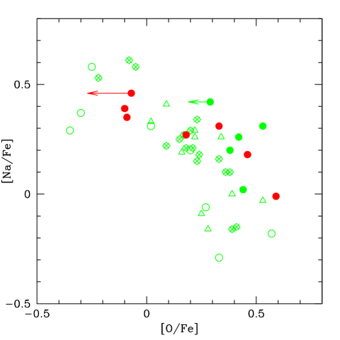
Figure 3: [Na/Fe] ratio as a function of [O/Fe], for stars in NGC6752. Red filled circles are our RGB bump stars in the present study. Green filled and open circles are subgiant and turn-off stars, respectively, from Carretta et al. (2005). Literature data are as follow: green diamonds with crosses inside are bright red giants from the extensive study by Yong et al. (2003), open green triangles are red giant stars from Norris and Da Costa (1995; 6 stars) and Carretta (1994; 4 stars).

5.5 O-Na anticorrelation

The O-Na anticorrelation in NGC6752 is well known from previous observations of both TO and subgiant stars (Gratton et al. 2001, Carretta et al. 2005), as well as red giants (Carretta 1994; Norris & Da Costa 1995; Yong et al. 2003). It is fully confirmed by the present data for RGB bump stars (see Figure 3). Figure 3 collects also all data available up to now, which clearly shows how an extensive O-Na anticorrelation can be seen along all evolutionary phases.

5.6 Abundance of other elements

Table 11 lists the average abundances obtained for various elements. Also in this case, solar abundances were as in Gratton et al. (2003a). In the same Table we also compare the abundances obtained in this paper with the analysis of Gratton et al. (2003a) and James et al. (2004). The comparison is very good for the best determined elements: we found clear overabundances of the $\alpha-$elements ([$\alpha$/Fe]=$+0.27\pm 0.01$), a small deficiency of Ni, and slight overabundance of Ba. We notice that NGC6752 closely trace the composition of the dissipative component considered by Gratton et al. (2003b), in agreement with its kinematics (Dinescu et al. 1999). The overabundance of $\alpha$-elements looks quite similar to those of other globular clusters (see e.g. Gratton et al. 2004).

Table 11: Element-to-element abundance ratios for individual stars, and averaged over the whole sample. For comparison, we also give the values found by Gratton et al. (2003a) or James et al. (2004).

Star	n	[O/Fe]I	n	[Na/Fe]I	n	[Mg/Fe]I	n	[Si/Fe]I	n	[Ca/Fe]I
25072	1	$-$0.09	2	+0.35	2	+0.41	3	+0.34	9	+0.29
26529	1	$-$0.10	2	+0.39	2	+0.41	2	+0.18	9	+0.37
30409	1	+0.46	2	+0.18	2	+0.60	3	+0.37	10	+0.43
30426	1	+0.18	2	+0.27	2	+0.41	3	+0.22	10	+0.38
34854	1	+0.33	2	+0.31	2	+0.69	3	+0.45	7	+0.43
37999	1	+0.59	1	$-$0.01	2	+0.52	4	+0.32	12	+0.34
39672	1	$<-$0.07	1	+0.46	2	+0.52	1	+0.31	6	+0.30
Average		+0.19		+0.29		+0.51		+0.31		+0.36
error		0.11		0.06		0.04		0.03		0.02
r.m.s.		0.28		0.16		0.11		0.09		0.06
compare to						+0.28				+0.31
Star	n	[Sc/Fe]II	n	[Ti/Fe]I	n	[Ni/Fe]I	n	[Ba/Fe]II	$[\alpha/Fe]$
25072	1	+0.26	1	+0.30	2	$-$0.15	2	+0.27	+0.34
26529	1	$-$0.04	1	+0.19	2	$-$0.14	2	+0.29	+0.29
30409	1	$-$0.01	2	+0.15	2	$-$0.11	2	+0.39	+0.39
30426			2	+0.17	2	$-$0.18	2	+0.45	+0.30
34854	1	+0.05			2	$-$0.21	2	+0.37	+0.44
37999	2	$-$0.04	2	+0.16	2	$-$0.25	2	+0.28	+0.34
39672					1	$-$0.32	2	+0.43	+0.33
Average		+0.06		+0.19		$-$0.19		+0.35	+0.35
error		0.05		0.03		0.03		0.03	0.02
r.m.s.		0.12		0.06		0.07		0.07	0.05
compare to		$-$0.06		+0.20		$-$0.11		+0.18	+0.27

6 CONCLUSIONS

We have shown that a single 1300 seconds exposure with FLAMES at VLT2 may provide accurate estimates of the reddening toward NGC6752, as well as of the chemical composition of the cluster (errors of 0.005 mag and of 0.02 dex respectively). Similar analyses may provide results of comparable accuracy for other globular clusters too on a uniform scale. While results of similar accuracy have been already obtained for a few clusters (including NGC6752), use of FLAMES allows to achieve such accuracies with much less (about a factor of 20) observing time. An extensive program over a large number of clusters may lead to large reductions of errors in age determinations for those clusters for which accurate distances could be obtained from either the main sequence fitting method, or even better from dynamical methods.

- (1) Alonso, A., Arribas, S. & Martinez-Roger, C. 1999 A&AS, 140, 261
- (2) Carretta, E. 1994. Ph.D. Thesis, Un. Padua.
- (3) Carretta, E., Gratton, R.G., Clementini, G., & Fusi Pecci, F. 2000, ApJ, 533, 215
- (4) Carretta, E., Gratton, R.G., Lucatello, S., Bragaglia, A., & Bonifacio, P. 2005, A&A, 433, 597
- (5) Cassisi, S., Salaris, M., & Irwin, A.W. 2003, ApJ, 588, 862
- (6) Castelli, F., Gratton, R.G., & Kurucz, R.L. 1997, A&A, 318, 841
- (7) Cayrel, R. 1988, in The Impact of Very High S/N Spectroscopy on Stellar Physics, IAU Synp. 132, ed. G. Cayrel de Strobel & M. Spite, Kluwer Academic Publishers, Dordrecht, p.345
- (8) Dinescu, D.L., Girard, T.M., van Altena, W.F. 1999, AJ, 117, 1792
- (9) Dubath, P., Meylan, G., & Mayor, M. 1997, A&A, 324, 505
- (10) Freedman, W.L., Madore, B.F., Gibson, B.K., Ferrarese, L., Kelson, D.D. et al. 2001, ApJ, 553, 47
- (11) Freeman, K., & Bland-Hawthorn, J. 2002, ARA&A, 40, 487
- (12) Fuhrmann, K. 1998, A&A, 338, 161
- (13) Gratton, R.G. 1988, Rome Obs. Preprint, 29
- (14) Gratton, R.G., Carretta, E., Matteucci, F., & Sneden, C. 1996, in Formation of the Galactic Halo…Inside and Out, H. Morrison & A. Sarajedini, eds., ASP Conf. Ser. 92, 307;
- (15) Gratton, R.G., Fusi Pecci, F., Carretta, E., Clementini, G., Corsi, C.E., & Lattanzi, M. 1997, ApJ 491, 749
- (16) Gratton, R.G., Carretta, E., Matteucci, F., & Sneden, C. 2000, A&A, 358, 671
- (17) Gratton, R.G., Bonifacio, P., Bragaglia, A., Carretta, E., Castellani, V. et al. 2001, A&A, 369, 87
- (18) Gratton, R.G., Bragaglia, A., Carretta, E., Clementini, G., Desidera, S., Grundahl, F., & Lucatello, S., 2003a, A&A, 408, 529
- (19) Gratton, R.G., Carretta, E., Claudi, R., Lucatello, S., & Barbieri, M. 2003b, A&A, 408, 529
- (20) Gratton, R.G., Sneden, C., & Carretta, E., 2004, ARA&A, 42, 385
- (21) Harris, W.E. 1996, AJ, 112, 1487
- (22) James, G., François, P. Bonifacio, P., Bragaglia, A., Carretta, E., et al. 2004, A&A, 414, 1071
- (23) Jimenez, R., Verde, L., Treu, T., & Stern, D. 2003, ApJ, 593, 622
- (24) Kurucz 1992, in The Stellar Populations of Galaxies, IAU Symp. 149, B. Barbuy & A. Renzini eds, Kluwer Academic Publishers, Dordrecht, p.225
- (25) Landman, D.A., Roussel-Duprè, R., & Tanigawa, G. 1982, ApJ, 261, 732
- (26) Loomis, C.G., McLean, B.J., Greene, G.R., & White, R.L. 2004, BAAS, 205, 9110
- (27) Magain, P., 1984, A&A, 134, 189
- (28) Momany, Y., Bedin, L. R., Cassisi, S., Piotto, G., Ortolani, S., Recio-Blanco, A., De Angeli, F., & Castelli, F. 2004, A&A, 420, 605
- (29) Norris, J., & Da Costa, G.S. 1995, ApJL, 441, 81
- (30) Pasquini, L., Avila, G., Blecha, A. et al., 2002, The Messenger No. 110, p. 1
- (31) Peebles, P.J.E., & Dicke, R.H. 1968, ApJ, 154, 891
- (32) Piotto, G., Bedin, L.R., Cassisi, S., et al. 2004, Mem. SAIt Suppl. 5, 71
- (33) Pont, F., Mayor, M., Turon, C., & Vandenberg, D.A. 1998, A&A, 329, 87
- (34) Rosenberg, A., Saviane, I., Piotto, G., & Aparicio, A. 1999, AJ, 118, 2306
- (35) Rutledge, G.A., Hesser, J.E., Stetson, P.B., Mateo, M., Simard, L., Bolte, M., Friel, F.D., & Copin, Y. 1997, PASP, 109, 883
- (36) Salaris, M., Riello, M., Cassis, S., & Piotto G. 2004, A&A, 420, 911
- (37) Schlegel, D.J., Finkbeiner, D.P., Davis, M. 1998, ApJ, 500, 525
- (38) Schweizer, F. & Seitzer, P. 1993, ApJ, 417, L29
- (39) Spergel, D.N., Verde, L., Peiris, H.V., Komatsu, E., Nolta, M.R., et al. 2003, ApJS, 148, 175
- (40) Thompson, I.B., Kaluzny, J., Pych, W., & Krzeminski, W. 1999, AJ, 118, 462
- (41) Webbink, R.F. 1988, in The Harlow-Shapley Symposium on Globular Cluster Systems in Galaxies, IAU Symp. 126, Dordrecht, Kluwer Ascademic Press, p. 49
- (42) Yong D., Grundahl, F., Lambert, D.L., Nissen, P.E., & Shetrone, M.D. 2003, A&A, 402, 985
- (43) Zacharias, N., Urban, S., Zacharias, M., Wycoff, G., Hall, D., Monet, D., & Rafferty, T. 2004, AJ, 127, 3043
- (44) Zinn, R. 1985, ApJ, 293, 424