THE PIECEWISE PARABOLIC METHOD FOR
MULTIDIMENSIONAL RELATIVISTIC FLUID DYNAMICS

Abstract

We present an extension of the Piecewise Parabolic Method to special relativistic fluid dynamics in multidimensions. The scheme is conservative, dimensionally unsplit, and suitable for a general equation of state. Temporal evolution is second-order accurate and employs characteristic projection operators; spatial interpolation is piece-wise parabolic making the scheme third-order accurate in smooth regions of the flow away from discontinuities. The algorithm is written for a general system of orthogonal curvilinear coordinates and can be used for computations in non-cartesian geometries. A non-linear iterative Riemann solver based on the two-shock approximation is used in flux calculation. In this approximation, an initial discontinuity decays into a set of discontinuous waves only implying that, in particular, rarefaction waves are treated as flow discontinuities. We also present a new and simple equation of state which approximates the exact result for the relativistic perfect gas with high accuracy. The strength of the new method is demonstrated in a series of numerical tests and more complex simulations in one, two and three dimensions.

1 INTRODUCTION

Highly energetic astrophysical phenomena are known to be, in many cases, relativistic in nature. A wide range of objects, in fact, exhibits a number of properties that can be accounted for only in the framework of the theory of special or general relativity: superluminal motion of relativistic jets in extragalactic radio sources (Begelman et al., 1984), jets and accretion flows around massive compact objects (Koide et al., 1999; Meier et al., 2001), pulsar winds (Del Zanna et al., 2004; Bogovalov et al., 2005), gamma ray bursts (Aloy et al., 2000; Zhang et al., 2003; Mizuno et al., 2004), as well as particle beams produced in heavy-ion collisions in terrestrial experiments (Ackermann et al., 2001; Morita et al., 2002; Molnar & Huovinen, 2004) characterized by flow velocities very close ($\gtrsim 0.99c$) to the speed of light. Such problems are difficult to study numerically due to inherent complexity of the problem itself exhibiting rapid spatial and temporal changes often demanding development of more efficient algorithms.

Recent progress in the development of powerful methods in computational fluid dynamics allowed researchers to gain understanding of relativistic flows. Numerical formulations of the special relativistic fluid equations have been investigated by several authors in the last decade (for an excellent review see Martí & Müller, 2003). However, there now exists strong evidence that a particular class of numerical methods, the so-called high-resolution shock-capturing schemes (HRSC henceforth, e.g., Donat et al., 1998; Marquina et al., 1992), provide the necessary means to develop stable and robust relativistic (special or general) fluid dynamics codes. HRSC methods rely on the conservative formulation of the fluid equations. This formulation is of fundamental importance in representing the evolution of flows with steep gradients and discontinuities. One of the key aspects of these schemes is the temporal evolution of the system, which routinely involves (exact or approximate) solution of Riemann problems at the interfaces separating numerical grid cells, thus making these schemes highly successful in modeling discontinuous flows. Besides, these algorithms have at least 2nd order accuracy in smooth regions of the flow and have been shown to produce excellent results for a wide variety of problems.

Shock-capturing schemes have a long standing tradition in the framework of solving the Euler equations of gas dynamics (e.g., Colella, 1985; Colella & Woodward, 1984; VanLeer, 1997; Toro, 1997). Several of these “classical” schemes have now been extended to special relativistic hydrodynamics (see Balsara, 1994; Dai & Woodward, 1997; Falle & Komissarov, 1996; Donat et al., 1998; Sokolov et al., 2001, and references therein). The Piecewise Parabolic Method (PPM) by Colella & Woodward (1984, CW84 henceforth) is still considered as the state-of-the-art method in computational fluid dynamics. The original PPM algorithm has been recently re-formulated for the relativistic fluid flows in one spatial dimension by Martí & Müller (1996). Here we present an extension of the PPM method to multidimensional relativistic hydrodynamics. As we will show, the main differences between the classical and relativistic version of PPM are the coupling between normal and transverse velocity components introduced by the Lorentz factor and the coupling of the latter to the specific enthalpy.

Our relativistic PPM consists of several components. The piece-wise parabolic interpolation is done in the volume coordinate (CW84) and provides third-order accuracy in space in smooth parts of the flow. Temporal evolution uses characteristic information and is second-order accurate. The scheme also uses a non-linear iterative Riemann solver based on the two-shock approximation. The unsplit fully-coupled corner-transport upwind method is used for advection (Colella, 1990; Saltzman, 1994). Several verifications tests are presented to demonstrate the correctness of the implementation.

The paper is organized as follows. In §2 we give a short review of the special relativistic fluid equations. In §3 we present discretization of the equations in a general system of orthogonal curvilinear coordinates and describe the numerical method. We include the details of the time evolution algorithm based on characteristic tracing. The Riemann solver is presented in §3.3. In §3.4 we consider different equation of states and introduce a new formulation suitable for relativistic regimes. Several numerical tests are presented in §4 and conclusions are drawn in §5.

2 THE EQUATIONS OF RELATIVISTIC HYDRODYNAMICS

In the framework of special relativity, the motion of an ideal fluid is governed by the laws of particle number conservation and energy-momentum conservation (Landau & Lifshitz, 1959; Weinberg, 1972). In the laboratory frame of reference, the conservation equations written in divergence form are

$$\frac{\partial}{\partial t}\left(\begin{array}[]{c}D\\ \boldsymbol{m}\\ E\end{array}\right)+\nabla\cdot\left(\begin{array}[]{c}D\boldsymbol{v}\\ \boldsymbol{m}\boldsymbol{v}+p\boldsymbol{I}\\ \boldsymbol{m}c^{2}\end{array}\right)=0\,,$$ (1)

where $\boldsymbol{v}$, $D$, $\boldsymbol{m}$, $E$ and $p$ define, respectively, the fluid three-velocity, density, momentum density, total energy density and pressure. In the local rest frame the fluid can be described in terms of its Lorentz-invariant thermodynamic quantities: the proper rest mass density $\rho$, specific enthalpy $h$, and pressure $p$. The transformation between the two frames of reference is given by

$$D=\displaystyle\gamma\rho\,,$$ (2)

$$\boldsymbol{m}=\displaystyle\rho h\gamma^{2}\frac{\boldsymbol{v}}{c^{2}}\,,$$ (3)

$$E=\displaystyle\rho h\gamma^{2}-p\,,$$ (4)

where $\gamma=\big{(}1-\boldsymbol{v}^{2}/c^{2}\big{)}^{-1/2}$ is the Lorentz factor and $c$ is the speed of light. The specific enthalpy, $h$, is related to the proper internal energy density, $e$, by

$$h=\frac{e+p}{\rho}\,.$$ (5)

An equation of state (EoS) provides an additional relation between thermodynamic quantities and allows to close the system of conservation laws (1). Here we assume, without loss of generality, that the EoS expresses the specific enthalpy $h$ as a function of the pressure $p$ and the specific proper volume $\tau=1/\rho$, i.e. $h=h(p,\tau)$. This allows us to define the sound speed $c_{s}$ as

$$\frac{c^{2}_{s}}{c^{2}}\equiv\left(\frac{\partial p}{\partial e}\right)_{s}=\frac{\tau^{2}}{h}\frac{\partial h}{\partial\tau}\left(\frac{\partial h}{\partial p}-\tau\right)^{-1}\,,$$ (6)

where the derivative in equation (6) has to be taken at constant entropy $s$:

$$dh|_{s}\equiv\left.\left(Tds+\frac{dp}{\rho}\right)\right|_{s}=\tau\,dp\,.$$ (7)

We will consider only causal EoS, i.e., those for which $c_{s}<c$. For such equations of state, the hyperbolic property of equations (1) is preserved (Anile, 1989). In §3.4 we provide explicit expressions for the sound speed for different EoS suitable for relativistic flows.

We describe the relativistic fluid in terms of the state vectors of conservative, $\boldsymbol{U}=(D,m_{1},m_{2},m_{3},E)$, and primitive, $\boldsymbol{V}=(\rho,v_{1},v_{2},v_{3},p)$, variables. Here, $m_{d}$ and $v_{d}$ ($d=1,2,3$) are the projection of the three-momentum $\boldsymbol{m}$ and three-velocity $\boldsymbol{v}$ vectors along the coordinate axis, that is, $m_{d}\equiv\hat{\boldsymbol{n}}_{d}\cdot\boldsymbol{m}$ and $v_{d}\equiv\hat{\boldsymbol{n}}_{d}\cdot\boldsymbol{v}$.

Equations (2)–(4) define the map $\boldsymbol{U}=\boldsymbol{U}(\boldsymbol{V})$; the inverse relation gives $\boldsymbol{V}$ in terms of $\boldsymbol{U}$:

$$\rho=\frac{D}{\gamma}\,,$$ (8)

$$\frac{\boldsymbol{v}}{c^{2}}=\frac{\boldsymbol{m}}{E+p}\,,$$ (9)

$$p=Dh\gamma-E\,.$$ (10)

This inverse map is not trivial due to the non-linearity introduced by the Lorentz factor $\gamma$. Using equation (9) one can express the Lorentz factor as a function of the pressure:

$$\frac{1}{\gamma^{2}(p)}=1-\frac{\boldsymbol{m}^{2}c^{2}}{\left(E+p\right)^{2}}\,.$$ (11)

If $D$, $\boldsymbol{m}$ and $E$ are given, equations (10) and (11) can be combined together to obtain an implicit expression for $p$:

$$f(p)=Dh\big{(}p,\tau(p)\big{)}\gamma(p)-E-p=0\,.$$ (12)

This equation must be solved numerically in order to recover the pressure from a set of conservative variables $\boldsymbol{U}$. Notice that $\tau=\tau(p)$ depends on the pressure $p$ through $\tau=\gamma(p)/D$ and that the specific enthalpy $h$ is, in general, function of both $p$ and $\tau$, $h=h(p,\tau(p))$.

If the Newton-Raphson method is used as the root finder for pressure, the derivative of equation (12) with respect to $p$ is needed. It can be expressed in terms of the derivatives of the specific enthalpy , already appearing in equation (6):

$$\frac{df(p)}{dp}=D\gamma\frac{\partial h}{\partial p}-\frac{\boldsymbol{m}^{2}c^{2}\gamma^{3}}{(E+p)^{3}}\left(\gamma\frac{\partial h}{\partial\tau}+Dh\right)-1\,.$$ (13)

Equations (8)–(10), together with the pressure equation (12), have to be solved at each time step in order to provide the map $\boldsymbol{V}(\boldsymbol{U})$ needed in our numerical method.

3 DESCRIPTION OF THE ALGORITHM

Till now we considered the system of conservation laws (1]) written in divergence form. However, this differential representation is valid as long as the flow remains smooth. Since hyperbolic systems of conservation laws also admit discontinuous solutions, we should consider the more general integral form of the equations. We proceed as follows.

We introduce a generic system of orthogonal curvilinear coordinates, $(x^{1},x^{2},x^{3})$, and define $\hat{\boldsymbol{n}}_{d}$ to be the unit vectors associated with the coordinate directions, $d=1,2,3$. Orthonormality requires $\hat{\boldsymbol{n}}_{d}\cdot\hat{\boldsymbol{n}}_{d^{\prime}}=1$ when $d=d^{\prime}$ and $\hat{\boldsymbol{n}}_{d}\cdot\hat{\boldsymbol{n}}_{d^{\prime}}=0$ otherwise. The geometrical properties are then described in terms of the scale factors $h_{1}$, $h_{2}$ and $h_{3}$ which are, in general, functions of the coordinates, i.e., $h_{d}\equiv h_{d}(x^{1},x^{2},x^{3})$. We divide our computational domain into control volumes,

$$\Delta\mathcal{V}_{ijk}=\int_{x^{1}_{i-\frac{1}{2}}}^{x^{1}_{i+\frac{1}{2}}}\int_{x^{2}_{j-\frac{1}{2}}}^{x^{2}_{j+\frac{1}{2}}}\int_{x^{3}_{k-\frac{1}{2}}}^{x^{3}_{k+\frac{1}{2}}}d\mathcal{V}\,,\quad d\mathcal{V}=h_{1}h_{2}h_{3}\,dx^{1}dx^{2}dx^{3}\,,$$ (14)

where the index triplet $(i,j,k)$ corresponds to the $\hat{\boldsymbol{n}}_{1}$, $\hat{\boldsymbol{n}}_{2}$ and $\hat{\boldsymbol{n}}_{3}$ directions. The integrals in equation (14) are evaluated between the lower ($x^{1}_{i-\frac{1}{2}},x^{2}_{j-\frac{1}{2}},x^{3}_{k-\frac{1}{2}}$) and upper ($x^{1}_{i+\frac{1}{2}},x^{2}_{j+\frac{1}{2}},x^{3}_{k+\frac{1}{2}}$) coordinate limits of the grid cell $ijk$, where

$$x^{1}_{i+\frac{1}{2}}-x^{1}_{i-\frac{1}{2}}=\Delta x^{1}_{i}\,,\quad x^{2}_{j+\frac{1}{2}}-x^{2}_{j-\frac{1}{2}}=\Delta x^{2}_{j}\,,\quad x^{3}_{k+\frac{1}{2}}-x^{3}_{k-\frac{1}{2}}=\Delta x^{3}_{k}\,,\quad$$ (15)

here $\Delta x^{1}_{i}$, $\Delta x^{2}_{j}$ and $\Delta x^{3}_{k}$ are the zone widths in the three coordinate directions.

We restrict our attention to those coordinate systems for which the volume defined by equation (14) can be represented as the product of three different functions, each one depending on one coordinate only, i.e.,

$$\Delta\mathcal{V}_{ijk}=\left(\xi^{1}(x^{1}_{i+\frac{1}{2}})-\xi^{1}(x^{1}_{i-\frac{1}{2}})\right)\left(\xi^{2}(x^{2}_{j+\frac{1}{2}})-\xi^{2}(x^{2}_{j-\frac{1}{2}})\right)\left(\xi^{3}(x^{3}_{k+\frac{1}{2}})-\xi^{3}(x^{3}_{k-\frac{1}{2}})\right)$$ (16)

The three functions $\xi^{1}(x^{1})$, $\xi^{2}(x^{2})$, and $\xi^{3}(x^{3})$ are the generalized volume coordinates. These coordinates allow us to define the volumetric centroids $\xi^{1}_{i}$, $\xi^{2}_{j}$, $\xi^{3}_{k}$ corresponding to the point $(x^{1}_{i},x^{2}_{j},x^{3}_{k})$ as

$$\xi^{1}_{i}\equiv\xi^{1}(x^{1}_{i})=\frac{\xi^{1}(x^{1}_{i+\frac{1}{2}})+\xi^{1}(x^{1}_{i-\frac{1}{2}})}{2}\,,$$ (17)

$$\xi^{2}_{j}\equiv\xi^{2}(x^{2}_{j})=\frac{\xi^{2}(x^{2}_{j+\frac{1}{2}})+\xi^{2}(x^{2}_{j-\frac{1}{2}})}{2}\,,$$ (18)

$$\xi^{3}_{k}\equiv\xi^{3}(x^{3}_{k})=\frac{\xi^{3}(x^{3}_{k+\frac{1}{2}})+\xi^{3}(x^{3}_{k-\frac{1}{2}})}{2}\,.$$ (19)

Notice that in Cartesian coordinates, $(\xi^{1},\xi^{2},\xi^{3})=(x,y,z)$, and the volumetric centroids coincide with the geometrical zone centers. In cylindrical geometry, $(x^{1},x^{2},x^{3})=(r,\phi,z)$, however,

$$\xi^{1}(r)=\frac{r^{2}}{2}\,,\quad\xi^{2}(\phi)=\phi\,,\quad\xi^{3}(z)=z\,,$$ (20)

with the locations corresponding to the volumetric centroids given by

$$r_{i}=\left(\frac{r^{2}_{i+\frac{1}{2}}+r^{2}_{i-\frac{1}{2}}}{2}\right)^{\frac{1}{2}}\,,\quad\phi_{j}=\frac{\phi_{j+\frac{1}{2}}+\phi_{j-\frac{1}{2}}}{2}\,,\quad z_{k}=\frac{z_{k+\frac{1}{2}}+z_{k-\frac{1}{2}}}{2}\,.$$ (21)

Similarly, in spherical coordinates, $(x^{1},x^{2},x^{3})=(r,\theta,\phi)$, one obtains

$$\xi^{1}(r)=\frac{r^{3}}{3}\,,\quad\xi^{2}(\theta)=1-\cos\theta\,,\quad\xi^{3}(\phi)=\phi\,,$$ (22)

and the corresponding locations of the volumetric centroids are

$$r_{i}=\left(\frac{r^{3}_{i+\frac{1}{2}}+r^{3}_{i-\frac{1}{2}}}{2}\right)^{\frac{1}{3}}\,,\quad\theta_{j}=\cos^{-1}\left(\frac{\cos\theta_{j+\frac{1}{2}}+\cos\theta_{j-\frac{1}{2}}}{2}\right)\,,\quad\phi_{k}=\frac{\phi_{k+\frac{1}{2}}+\phi_{k-\frac{1}{2}}}{2}\,.$$ (23)

The areas of the zone faces are expressed by $A^{d}=\int\hat{\boldsymbol{n}}_{d}\cdot d\boldsymbol{A}$, where $d\boldsymbol{A}$ is the area element $d\boldsymbol{A}=dA^{1}\hat{\boldsymbol{n}}_{1}+dA^{2}\hat{\boldsymbol{n}}_{2}+dA^{3}\hat{\boldsymbol{n}}_{3}$, and $dA^{d}\equiv d\mathcal{V}/(h_{d}\,dx^{d})$. The result written in expanded form is

$$A^{1}_{i\pm\frac{1}{2},j,k}=\int_{x^{2}_{j-\frac{1}{2}}}^{x^{2}_{j+\frac{1}{2}}}\int_{x^{3}_{k-\frac{1}{2}}}^{x^{3}_{k+\frac{1}{2}}}h_{2}(x^{1}_{i\pm\frac{1}{2}},x^{2},x^{3})h_{3}(x^{1}_{i\pm\frac{1}{2}},x^{2},x^{3})\,dx^{2}dx^{3}\,,$$ (24)

$$A^{2}_{i,j\pm\frac{1}{2},k}=\int_{x^{1}_{i-\frac{1}{2}}}^{x^{1}_{i+\frac{1}{2}}}\int_{x^{3}_{k-\frac{1}{2}}}^{x^{3}_{k+\frac{1}{2}}}h_{1}(x^{1},x^{2}_{j\pm\frac{1}{2}},x^{3})h_{3}(x^{1},x^{2}_{j\pm\frac{1}{2}},x^{3})\,dx^{1}dx^{3}\,,$$ (25)

$$A^{3}_{i,j,k\pm\frac{1}{2}}=\int_{x^{1}_{i-\frac{1}{2}}}^{x^{1}_{i+\frac{1}{2}}}\int_{x^{2}_{j-\frac{1}{2}}}^{x^{2}_{j+\frac{1}{2}}}h_{1}(x^{1},x^{2},x^{3}_{k\pm\frac{1}{2}})h_{2}(x^{1},x^{2},x^{3}_{k\pm\frac{1}{2}})\,dx^{1}dx^{2}\,.$$ (26)

Explicit expressions for the scale factors and face areas are given in Appendix A.

Finally, the facial quadrature points located on the opposite bounding faces,

$$\left(x^{1}_{i\pm\frac{1}{2}},x^{2}_{j},x^{3}_{k}\right)\,,\quad\left(x^{1}_{i},x^{2}_{j\pm\frac{1}{2}},x^{3}_{k}\right)\,,\quad\left(x^{1}_{i},x^{2}_{j},x^{3}_{k\pm\frac{1}{2}}\right)\,,\quad$$ (27)

are used to compute the arc length separation,

$$\Delta l^{1}_{ijk}=\int_{x^{1}_{i-\frac{1}{2}}}^{x^{1}_{i+\frac{1}{2}}}h_{1}(x^{1},x^{2}_{j},x^{3}_{k})dx^{1}\,.$$ (28)

Similar expressions can be given for $\Delta l^{2}_{ijk}$ and $\Delta l^{3}_{ijk}$.

The integral form of the equations can now be obtained by integrating the system (1) over a computational volumes $\Delta\mathcal{V}_{ijk}$ and over a discrete time interval $\Delta t^{n}\equiv t^{n+1}-t^{n}$. Using Gauss’s theorem, the evolutionary equations provide a relation between the volume averaged conserved quantities and the time-averaged surface integrals for the divergence terms:

$$\bar{D}^{n+1}_{ijk}-\bar{D}^{n}_{ijk}=-\frac{\Delta t^{n}}{\Delta\mathcal{V}_{ijk}}\oint_{ijk}\left<D\boldsymbol{v}\right>^{n}\cdot d\boldsymbol{A}\,,$$ (29)

$$\bar{m}^{n+1}_{d,ijk}-\bar{m}^{n}_{d,ijk}=-\frac{\Delta t^{n}}{\Delta\mathcal{V}_{ijk}}\left[\oint_{ijk}\left<m_{d}\boldsymbol{v}\right>^{n}\cdot d\boldsymbol{A}+\int_{ijk}\hat{\boldsymbol{n}}_{d}\cdot\left<\nabla p+\boldsymbol{S}_{G}\big{(}\boldsymbol{m}\boldsymbol{v}\big{)}\right>^{n}d\mathcal{V}\right]\,,$$ (30)

$$\bar{E}^{n+1}_{ijk}-\bar{E}^{n}_{ijk}=-\frac{\Delta t^{n}}{\Delta\mathcal{V}_{ijk}}\oint_{ijk}\left<\boldsymbol{m}\right>^{n}\cdot d\boldsymbol{A}\,,$$ (31)

where $d=1,2,3$ enumerate coordinate directions and the speed of light $c$ has been set equal to unity, a convention to be used for the rest of this paper. Equations (29)–(31) express conservation of mass, momentum, and energy. In the equations above an overbar symbol denotes a volume average,

$$\bar{D}^{n}_{ijk}\equiv\frac{1}{\Delta\mathcal{V}_{ijk}}\int_{ijk}D(x^{1},x^{2},x^{3},t^{n})\,d\mathcal{V}\,,$$ (32)

while a bracket denotes a time-averaged quantity,

$$\left<D\boldsymbol{v}\right>^{n}\equiv\frac{1}{\Delta t^{n}}\int_{t^{n}}^{t^{n+1}}D(x^{1},x^{2},x^{3},t)\boldsymbol{v}(x^{1},x^{2},x^{3},t)\,dt\,.$$ (33)

Notice that expressions (29)–(30) are exact and no approximation has been introduced so far.

The vector $\boldsymbol{S}_{G}(\boldsymbol{m}\boldsymbol{v})$ accounts for geometrical source terms arising from taking the divergence of the dyad $\boldsymbol{m}\boldsymbol{v}$ in a curvilinear system of coordinates (explicit expressions for the geometrical source terms are given in Appendix A).

3.1 Evolution in Multi-dimensions

Equations (29)–(31) are integrated by first solving the homogeneous problem, i.e. without the source term $\boldsymbol{S}_{G}$ in equation [30], separately from a source step.

Let $\boldsymbol{\mathcal{H}}^{\Delta t}$ be the solution operator corresponding to the homogeneous part of the problem and $\boldsymbol{\mathcal{S}}^{\Delta t}$ be the operator describing the contribution of the source step over the time step $\Delta t$. Starting from the initial data, $\bar{\boldsymbol{U}}^{n}$, the solution for the next two time levels is computed using operator splitting (Strang, 1968):

$$\bar{\boldsymbol{U}}^{n+1}=\boldsymbol{\mathcal{S}}^{\Delta t}\boldsymbol{\mathcal{H}}^{\Delta t}\left(\bar{\boldsymbol{U}}^{n}\right)\,,$$ (34)

whereas

$$\bar{\boldsymbol{U}}^{n+2}=\boldsymbol{\mathcal{H}}^{\Delta t}\boldsymbol{\mathcal{S}}^{\Delta t}\left(\bar{\boldsymbol{U}}^{n+1}\right)\,,$$ (35)

Notice that this approach is second-order accurate in time, provided that the two operators have at least the same order of accuracy and the same time step is used for two consecutive levels.

The homogeneous operator $\boldsymbol{\mathcal{H}}^{\Delta t}$ is based on the spatially unsplit fully corner-coupled method (CTU, Colella, 1990; Saltzman, 1994; Miller & Colella, 2001, 2002). The conservative update results from acting $\boldsymbol{\mathcal{H}}^{\Delta t}$ on $\bar{\boldsymbol{U}}^{n}$:

$$\boldsymbol{\mathcal{H}}^{\Delta t}\left(\bar{\boldsymbol{U}}^{n}\right)=\bar{\boldsymbol{U}}^{n}+\boldsymbol{\mathcal{L}}^{1}\left(\boldsymbol{U}^{n+\frac{1}{2}}_{i+\frac{1}{2}},\boldsymbol{U}^{n+\frac{1}{2}}_{i-\frac{1}{2}}\right)+\boldsymbol{\mathcal{L}}^{2}\left(\boldsymbol{U}^{n+\frac{1}{2}}_{j+\frac{1}{2}},\boldsymbol{U}^{n+\frac{1}{2}}_{j-\frac{1}{2}}\right)+\boldsymbol{\mathcal{L}}^{3}\left(\boldsymbol{U}^{n+\frac{1}{2}}_{k+\frac{1}{2}},\boldsymbol{U}^{n+\frac{1}{2}}_{k-\frac{1}{2}}\right)\,,$$ (36)

where $\bar{\boldsymbol{U}}^{n}=\left(\bar{D}_{ijk},\bar{\boldsymbol{m}}_{ijk},\bar{E}_{ijk}\right)^{n}$ is a state vector of volume-averaged conserved quantities at time $t=t^{n}$. Here we adopted the convention in which the integer-valued subscripts $i,j,k$ are omitted when referring to three-dimensional quantities while the half integer values are used to denote zone edges. The same convention is used throughout the rest of the paper.

The last three terms in equation (36), $\boldsymbol{\mathcal{L}}^{d}$, represent one-dimensional flux-differencing operators, where $d=1,2,3$ labels directions. For $d=1$ (expressions for $d=2$ and $d=3$ are obtained by suitable permutations of indices) one has

$$\begin{split}\boldsymbol{\mathcal{L}}^{1}\left(\boldsymbol{U}^{n+\frac{1}{2}}_{i+\frac{1}{2}},\boldsymbol{U}^{n+\frac{1}{2}}_{i-\frac{1}{2}}\right)=&-\frac{\Delta t}{\Delta\mathcal{V}}\left[\boldsymbol{F}^{1}\left(\boldsymbol{U}^{n+\frac{1}{2}}_{i+\frac{1}{2}}\right)A^{1}_{i+\frac{1}{2}}-\boldsymbol{F}^{1}\left(\boldsymbol{U}^{n+\frac{1}{2}}_{i-\frac{1}{2}}\right)A^{1}_{i-\frac{1}{2}}\right]\\ &-\frac{\Delta t}{\Delta l^{1}}\left[\boldsymbol{P}^{1}\left(\boldsymbol{U}^{n+\frac{1}{2}}_{i+\frac{1}{2}}\right)-\boldsymbol{P}^{1}\left(\boldsymbol{U}^{n+\frac{1}{2}}_{i-\frac{1}{2}}\right)\right]\,,\end{split}$$ (37)

where

$$\boldsymbol{F}^{1}(\boldsymbol{U})=\left(\begin{array}[]{c}Dv_{1}\\ m_{1}v_{1}\\ m_{2}v_{1}\\ m_{3}v_{1}\\ m_{1}\end{array}\right)\,,$$ (38)

is the flux vector, and

$$\boldsymbol{P}^{1}(\boldsymbol{U})=\left(\begin{array}[]{c}0\\ p\\ 0\\ 0\\ 0\end{array}\right)\,,$$ (39)

is the pressure term. The state vectors $\boldsymbol{U}^{n+\frac{1}{2}}_{i\pm\frac{1}{2}}$ are solutions to Riemann problems with suitable time-centered left and right states properly computed at each facial quadrature point. For example,

$$\boldsymbol{U}^{n+\frac{1}{2}}_{i+\frac{1}{2}}=\boldsymbol{\mathcal{R}}\left(\boldsymbol{U}^{n+\frac{1}{2}}_{i+\frac{1}{2},L},\boldsymbol{U}^{n+\frac{1}{2}}_{i+\frac{1}{2},R}\right)\,,$$ (40)

where $\boldsymbol{\mathcal{R}}(\cdot,\cdot)$ denotes the solution to the Riemann problem (see §3.3 for details).

In the three-dimensional case, the conservative update (36) involves the following four steps. In the first predictor step we construct initial left and right states just as in the one-dimensional case. In the second predictor step the initial states are corrected for contributions from transverse directions to form secondary predictors. These secondary predictors are used in the third step to calculate the fully corner coupled states. Finally, the fluxes required by the conservative update follow from the solutions of Riemann problems with the fully corner-coupled states used as input. In what follows we present the details of this procedure.

The starting point for the construction of the input left and right states to the Riemann problems is the predictor step described in §3.2 below. In this step we use Taylor expansion to obtain edge- and time-centered estimates for the left and right states $\hat{\boldsymbol{U}}^{n+\frac{1}{2}}_{i+\frac{1}{2},L}$ and $\hat{\boldsymbol{U}}^{n+\frac{1}{2}}_{i+\frac{1}{2},R}$.

Next the following 6 secondary predictors are calculated:

$$\left.\begin{array}[]{c}\displaystyle\boldsymbol{U}^{{}^{\prime}1}_{j\pm\frac{1}{2},S}=\hat{\boldsymbol{U}}^{n+\frac{1}{2}}_{j\pm\frac{1}{2},S}\\ \vskip 6.0pt plus 2.0pt minus 2.0pt\cr\displaystyle\boldsymbol{U}^{{}^{\prime}1}_{k\pm\frac{1}{2},S}=\hat{\boldsymbol{U}}^{n+\frac{1}{2}}_{k\pm\frac{1}{2},S}\end{array}\right\}+\frac{1}{3}\boldsymbol{\mathcal{L}}^{1}\left(\hat{\boldsymbol{U}}^{n+\frac{1}{2}}_{i+\frac{1}{2}},\hat{\boldsymbol{U}}^{n+\frac{1}{2}}_{i-\frac{1}{2}}\right)\,,$$ (41)

$$\left.\begin{array}[]{c}\displaystyle\boldsymbol{U}^{{}^{\prime}2}_{i\pm\frac{1}{2},S}=\hat{\boldsymbol{U}}^{n+\frac{1}{2}}_{i\pm\frac{1}{2},S}\\ \vskip 6.0pt plus 2.0pt minus 2.0pt\cr\displaystyle\boldsymbol{U}^{{}^{\prime}2}_{k\pm\frac{1}{2},S}=\hat{\boldsymbol{U}}^{n+\frac{1}{2}}_{k\pm\frac{1}{2},S}\end{array}\right\}+\frac{1}{3}\boldsymbol{\mathcal{L}}^{2}\left(\hat{\boldsymbol{U}}^{n+\frac{1}{2}}_{j+\frac{1}{2}},\hat{\boldsymbol{U}}^{n+\frac{1}{2}}_{j-\frac{1}{2}}\right)\,,$$ (42)

$$\left.\begin{array}[]{c}\displaystyle\boldsymbol{U}^{{}^{\prime}3}_{i\pm\frac{1}{2},S}=\hat{\boldsymbol{U}}^{n+\frac{1}{2}}_{i\pm\frac{1}{2},S}\\ \vskip 6.0pt plus 2.0pt minus 2.0pt\cr\displaystyle\boldsymbol{U}^{{}^{\prime}3}_{j\pm\frac{1}{2},S}=\hat{\boldsymbol{U}}^{n+\frac{1}{2}}_{j\pm\frac{1}{2},S}\end{array}\right\}+\frac{1}{3}\boldsymbol{\mathcal{L}}^{3}\left(\hat{\boldsymbol{U}}^{n+\frac{1}{2}}_{k+\frac{1}{2}},\hat{\boldsymbol{U}}^{n+\frac{1}{2}}_{k-\frac{1}{2}}\right)\,,$$ (43)

where we adopt the convention that $S=L$ at $i+\frac{1}{2}$ and $S=R$ at $i-\frac{1}{2}$ (similar formulae are obtained for $j\pm\frac{1}{2}$, $k\pm\frac{1}{2}$).

The flux differencing operators on the right hand side of equations (41)–(43) are obtained by solving Riemann problems with the states obtained in the first corrector step, e.g.,

$$\hat{\boldsymbol{U}}^{n+\frac{1}{2}}_{i+\frac{1}{2}}=\boldsymbol{\mathcal{R}}\left(\hat{\boldsymbol{U}}^{n+\frac{1}{2}}_{i+\frac{1}{2},L},\hat{\boldsymbol{U}}^{n+\frac{1}{2}}_{i+\frac{1}{2},R}\right)\,.$$ (44)

In the third step we obtain the fully corner-coupled states,

$$\boldsymbol{U}^{n+\frac{1}{2}}_{i\pm\frac{1}{2},S}=\hat{\boldsymbol{U}}^{n+\frac{1}{2}}_{i\pm\frac{1}{2},S}+\frac{1}{2}\left[\boldsymbol{\mathcal{L}}^{2}\left(\boldsymbol{U}^{{}^{\prime}3}_{j+\frac{1}{2}},\boldsymbol{U}^{{}^{\prime}3}_{j-\frac{1}{2}}\right)+\boldsymbol{\mathcal{L}}^{3}\left(\boldsymbol{U}^{{}^{\prime}2}_{k+\frac{1}{2}},\boldsymbol{U}^{{}^{\prime}2}_{k-\frac{1}{2}}\right)\right]\,,$$ (45)

$$\boldsymbol{U}^{n+\frac{1}{2}}_{j\pm\frac{1}{2},S}=\hat{\boldsymbol{U}}^{n+\frac{1}{2}}_{j\pm\frac{1}{2},S}+\frac{1}{2}\left[\boldsymbol{\mathcal{L}}^{3}\left(\boldsymbol{U}^{{}^{\prime}1}_{k+\frac{1}{2}},\boldsymbol{U}^{{}^{\prime}1}_{k-\frac{1}{2}}\right)+\boldsymbol{\mathcal{L}}^{1}\left(\boldsymbol{U}^{{}^{\prime}3}_{i+\frac{1}{2}},\boldsymbol{U}^{{}^{\prime}3}_{i-\frac{1}{2}}\right)\right]\,,$$ (46)

$$\boldsymbol{U}^{n+\frac{1}{2}}_{k\pm\frac{1}{2},S}=\hat{\boldsymbol{U}}^{n+\frac{1}{2}}_{k\pm\frac{1}{2},S}+\frac{1}{2}\left[\boldsymbol{\mathcal{L}}^{1}\left(\boldsymbol{U}^{{}^{\prime}2}_{i+\frac{1}{2}},\boldsymbol{U}^{{}^{\prime}2}_{i-\frac{1}{2}}\right)+\boldsymbol{\mathcal{L}}^{2}\left(\boldsymbol{U}^{{}^{\prime}1}_{j+\frac{1}{2}},\boldsymbol{U}^{{}^{\prime}1}_{j-\frac{1}{2}}\right)\right]\,.$$ (47)

As in the previous step, quantities appearing in the flux differencing follow the solution of appropriate Riemann problems. For example,

$$\boldsymbol{U}^{{}^{\prime}1}_{j+\frac{1}{2}}=\boldsymbol{\mathcal{R}}\left(\boldsymbol{U}^{{}^{\prime}1}_{j+\frac{1}{2},L},\boldsymbol{U}^{{}^{\prime}1}_{j+\frac{1}{2},R}\right)\,.$$ (48)

The final step is the conservative update in which we use the fluxes obtained by solving Riemann problems with the fully corner-coupled states (eq. [45]–[47]).

In three dimensions a total of 12 Riemann problems are required: 3 to obtain the secondary predictors (eq. [41]–[43]), 6 to obtain the fully corner-coupled states (eq. [45]–[47]), and 3 necessary for the conservative update (eq. [36]). The six secondary predictors, equations (41)–(43), are not required in two dimensions and the fully corner-coupled states become

$$\boldsymbol{U}^{n+\frac{1}{2}}_{i\pm\frac{1}{2},S}=\hat{\boldsymbol{U}}^{n+\frac{1}{2}}_{i\pm\frac{1}{2},S}+\frac{1}{2}\boldsymbol{\mathcal{L}}^{2}\left(\hat{\boldsymbol{U}}^{n+\frac{1}{2}}_{j+\frac{1}{2}},\hat{\boldsymbol{U}}^{n+\frac{1}{2}}_{j-\frac{1}{2}}\right)\,,$$ (49)

$$\boldsymbol{U}^{n+\frac{1}{2}}_{j\pm\frac{1}{2},S}=\hat{\boldsymbol{U}}^{n+\frac{1}{2}}_{j\pm\frac{1}{2},S}+\frac{1}{2}\boldsymbol{\mathcal{L}}^{1}\left(\hat{\boldsymbol{U}}^{n+\frac{1}{2}}_{i+\frac{1}{2}},\hat{\boldsymbol{U}}^{n+\frac{1}{2}}_{i-\frac{1}{2}}\right)\,.$$ (50)

Therefore, in 2D, the conservative update involves the solution of 4 Riemann problems: 2 in the predictor step and 2 in the corrector step.

Contribution from geometrical source terms is included by solving the ordinary differential equation

$$\frac{d\boldsymbol{U}}{dt}=\boldsymbol{S}_{G}(\boldsymbol{U})\,,$$ (51)

with the solution from the previous step (either advection or possibly source term calculation if Strang splitting is used) used as the initial data. The solution is obtained with a second-order Runge-Kutta algorithm, and can be written in operator form as

$$\begin{array}[]{c}\displaystyle\boldsymbol{\mathcal{S}}^{\Delta t}\left(\boldsymbol{U}\right)=\frac{1}{2}\left[\boldsymbol{U}+\boldsymbol{U}^{*}+\Delta t\boldsymbol{S}_{G}\left(\boldsymbol{U}^{*}\right)\right]\,,\\ \vskip 6.0pt plus 2.0pt minus 2.0pt\cr\displaystyle\boldsymbol{U}^{*}=\boldsymbol{U}+\Delta t\boldsymbol{S}_{G}\left(\boldsymbol{U}\right)\,.\end{array}$$ (52)

Finally, the choice of the time step $\Delta t$ is based on the Courant-Friederichs-Lewy (CFL) condition (Courant et al., 1928):

$$\Delta t=C_{a}\times\min_{i,j,k}\left(\frac{\Delta l_{ijk}^{1}}{|\lambda_{\max}^{1}|},\frac{\Delta l_{ijk}^{2}}{|\lambda_{\max}^{2}|},\frac{\Delta l_{ijk}^{3}}{|\lambda_{\max}^{3}|}\right)\,.$$ (53)

Here $\lambda_{\max}^{d}$ is the fastest wave speed in the $\hat{\boldsymbol{n}}_{d}$ direction, and $0<C_{a}<1$ is the limiting factor.

3.2 The predictor step

In what follows we provide a detailed description of the predictor step which constitutes the first step in the multi-stage procedure described above. For simplicity we describe the operator applied to the first coordinate direction; modifications required for other directions are straightforward. The predictor step is comprised of the reconstruction algorithm followed by the calculation of left and right states at the zone interfaces. These states are used as input data to the Riemann problems in the second predictor step (eq. [41]–[43]) and are required in the construction of the fully corner coupled states, equations (45)–(47) in 3-D and equations (49), (50) in 2-D. Throughout this section we make use of the following abbreviations: $x=x^{1}$, $\xi=\xi^{1}$, $h=h^{1}$ and $A=A^{1}$.

During the reconstruction step a quartic polynomial is passed through the volume-averaged values $\bar{\boldsymbol{U}}^{n}_{i}$. The polynomial provides interface values for the hydrodynamic variables, $\boldsymbol{V}^{n}_{i+\frac{1}{2},S}$ ($S=L,R$) which are fourth-order accurate in space in smooth regions of the flow. The interpolation may be done either in the volume coordinate $\xi$ (CW84) or in the spatial coordinate $x$ (Blondin & Lufkin, 1993). Here we follow the former prescription and the details are given in Appendix B.

Once the interpolated zone-edge values are provided, we define a one-dimensional piece-wise parabolic profile inside each cell $i$:

$$\boldsymbol{V}^{n}(\xi)=\boldsymbol{V}^{n}_{i-\frac{1}{2},R}+\frac{\xi-\xi_{i-\frac{1}{2}}}{\Delta\xi_{i}}\left[\Delta\boldsymbol{V}^{n}_{i}+\boldsymbol{V}^{n}_{6i}\left(1-\frac{\xi-\xi_{i-\frac{1}{2}}}{\Delta\xi_{i}}\right)\right]\quad\textrm{for}\quad\xi_{i-\frac{1}{2}}\leq\xi\leq\xi_{i+\frac{1}{2}}\,,$$ (54)

where

$$\Delta\boldsymbol{V}^{n}_{i}=\boldsymbol{V}^{n}_{i+\frac{1}{2},L}-\boldsymbol{V}^{n}_{i-\frac{1}{2},R}\,,\quad\boldsymbol{V}_{6i}^{n}=6\left(\boldsymbol{V}^{n}_{i}-\frac{\boldsymbol{V}^{n}_{i+\frac{1}{2},L}+\boldsymbol{V}^{n}_{i-\frac{1}{2},R}}{2}\right)\,.$$ (55)

Notice, however, that when the interpolation is done in the spatial coordinate $x$ rather than in the volume coordinate $\xi$, equation (54) has to be modified by replacing $\xi(x)$ with $x$. Moreover, the definition of $\boldsymbol{V}_{6i}$ becomes geometry dependent (Blondin & Lufkin, 1993).

Second-order accuracy in time is obtained by considering the one-dimensional relativistic equations in quasi-linear form (derived for the one-dimensional case by Martí & Müller, 1996):

$$\frac{\partial\boldsymbol{V}}{\partial t}+\frac{1}{h}\boldsymbol{A}(\boldsymbol{V})\cdot\frac{\partial\boldsymbol{V}}{\partial x}=\boldsymbol{S}(\boldsymbol{V})\,.$$

Here

$$\boldsymbol{V}=\left(\begin{array}[]{c}\rho\\ v_{1}\\ v_{2}\\ v_{3}\\ p\end{array}\right)\,,\quad\boldsymbol{S}(\boldsymbol{V})=\frac{v_{1}}{\Delta^{2}}\frac{\partial}{\partial\xi}\left(\frac{1}{h}\frac{\partial\xi}{\partial x}\right)\left(\begin{array}[]{c}-\rho\\ v_{1}c_{s}^{2}/\gamma^{2}\\ v_{2}c_{s}^{2}/\gamma^{2}\\ v_{3}c_{s}^{2}/\gamma^{2}\\ -\rho hc_{s}^{2}\end{array}\right)\,,$$ (56)

are, respectively, the vector of primitive variables and geometrical sources, while

$$\boldsymbol{A}(\boldsymbol{V})=\frac{1}{\Delta^{2}}\left(\begin{array}[]{ccccc}v_{1}\Delta^{2}&\rho&0&0&\displaystyle-\frac{v_{1}}{h\gamma^{2}}\\ \vskip 6.0pt plus 2.0pt minus 2.0pt\cr 0&v_{1}(1-c_{s}^{2})&0&0&\displaystyle\frac{\eta^{2}}{\rho h\gamma^{2}}\\ \vskip 6.0pt plus 2.0pt minus 2.0pt\cr 0&\displaystyle-\frac{v_{2}c_{s}^{2}}{\gamma^{2}}&v_{1}\Delta^{2}&0&\displaystyle-\frac{v_{1}v_{2}\left(1-c_{s}^{2}\right)}{\rho h\gamma^{2}}\\ \vskip 6.0pt plus 2.0pt minus 2.0pt\cr 0&\displaystyle-\frac{v_{3}c_{s}^{2}}{\gamma^{2}}&0&v_{1}\Delta^{2}&\displaystyle-\frac{v_{1}v_{3}\left(1-c_{s}^{2}\right)}{\rho h\gamma^{2}}\\ \vskip 6.0pt plus 2.0pt minus 2.0pt\cr 0&\rho hc_{s}^{2}&0&0&v_{1}(1-c_{s}^{2})\end{array}\right)\,,$$ (57)

is the Jacobian, $\Delta^{2}=1-\boldsymbol{v}^{2}c_{s}^{2}$ and $\eta^{2}=1-v_{1}^{2}-c_{s}^{2}(v_{2}^{2}+v_{3}^{2})$.

The left and right states $\hat{\boldsymbol{V}}^{n+\frac{1}{2}}_{i+\frac{1}{2},L}$ and $\hat{\boldsymbol{V}}^{n+\frac{1}{2}}_{i-\frac{1}{2},R}$, are computed using the characteristic information carried to the zone edges $\xi_{i\pm\frac{1}{2}}$ by each family of waves emanating from the zone center during a single time step $\Delta t$. Firstly, for each characteristic $\#$ we find the domain of dependence for each interface:

$$\xi^{\#}_{i-\frac{1}{2},R}=\xi\left(x_{i-\frac{1}{2}}+\Delta x^{\#}_{i-\frac{1}{2}}\right)\,,\quad\xi^{\#}_{i+\frac{1}{2},L}=\xi\left(x_{i+\frac{1}{2}}-\Delta x^{\#}_{i+\frac{1}{2}}\right)\,,$$ (58)

where $\Delta x^{\#}_{i-\frac{1}{2}}$ and $\Delta x^{\#}_{i+\frac{1}{2}}$ are defined through

$$\int_{x_{i-\frac{1}{2}}}^{x_{i-\frac{1}{2}}+\Delta x^{\#}_{i-\frac{1}{2}}}h(x,x^{2}_{j},x^{3}_{k})dx=\Delta t\,\max(0,-\lambda^{\#}_{i})\,,$$ (59)

$$\int_{x_{i+\frac{1}{2}}-\Delta x^{\#}_{i+\frac{1}{2}}}^{x_{i+\frac{1}{2}}}h(x,x^{2}_{j},x^{3}_{k})dx=\Delta t\,\max(0,\lambda^{\#}_{i})\,.$$ (60)

Here $\#=\{+,0^{(1,2,3)},-\}$ labels the characteristic field, and $\lambda^{\#}$ is the corresponding eigenvalue (Falle & Komissarov, 1996; Donat et al., 1998),

$$\lambda^{-}=\frac{\gamma v_{1}\left(1-c_{s}^{2}\right)-c_{s}\eta}{\gamma\Delta^{2}}\,,\quad\lambda^{0^{(1,2,3)}}=v_{1}\,,\quad\lambda^{+}=\frac{\gamma v_{1}\left(1-c_{s}^{2}\right)+c_{s}\eta}{\gamma\Delta^{2}}\,.$$ (61)

As in classical hydrodynamics, the characteristics consist of two genuinely non-linear fields $\#=+,-$ and three linearly degenerate fields $\#=0^{(1,2,3)}$. Also, note that in cylindrical or spherical coordinates, $h\equiv h^{1}(x^{2}_{j},x^{3}_{k})$ does not depend on $x$ and therefore $\Delta x^{\#}_{i\pm\frac{1}{2}}=\Delta t\,\max(0,\pm\lambda^{\#}_{i})/h(x^{2}_{j},x^{3}_{k})$.

Next, we calculate the average of $\boldsymbol{V}(\xi)$ over the domain of dependence lying to the left (for $\hat{\boldsymbol{V}}^{n+\frac{1}{2}}_{i+\frac{1}{2},L}$) or to the right (for $\hat{\boldsymbol{V}}^{n+\frac{1}{2}}_{i-\frac{1}{2},R}$) of the interface:

$$\boldsymbol{V}^{\#}_{i+\frac{1}{2},L}=\frac{1}{\xi_{i+\frac{1}{2}}-\xi^{\#}_{i+\frac{1}{2},L}}\int^{\xi_{i+\frac{1}{2}}}_{\xi^{\#}_{i+\frac{1}{2},L}}\boldsymbol{V}^{n}(\xi)d\xi\,,\quad\boldsymbol{V}^{\#}_{i-\frac{1}{2},R}=\frac{1}{\xi^{\#}_{i-\frac{1}{2},R}-\xi_{i-\frac{1}{2}}}\int^{\xi^{\#}_{i-\frac{1}{2},R}}_{\xi_{i-\frac{1}{2}}}\boldsymbol{V}^{n}(\xi)d\xi\,.$$ (62)

The zone averages are obtained by straightforward integration of the parabolic zone profiles (eq. [54]):

$$\boldsymbol{V}^{\#}_{i+\frac{1}{2},L}=\boldsymbol{V}^{n}_{i+\frac{1}{2},L}-\frac{\xi_{i+\frac{1}{2}}-\xi^{\#}_{i+\frac{1}{2},L}}{2\Delta\xi_{i}}\left[\Delta\boldsymbol{V}^{n}_{i}-\boldsymbol{V}^{n}_{6i}\left(1-\frac{2}{3}\frac{\xi_{i+\frac{1}{2}}-\xi^{\#}_{i+\frac{1}{2},L}}{\Delta\xi_{i}}\right)\right]\,,$$ (63)

$$\boldsymbol{V}^{\#}_{i-\frac{1}{2},R}=\boldsymbol{V}^{n}_{i-\frac{1}{2},R}+\frac{\xi^{\#}_{i-\frac{1}{2},R}-\xi_{i-\frac{1}{2}}}{2\Delta\xi_{i}}\left[\Delta\boldsymbol{V}^{n}_{i}+\boldsymbol{V}^{n}_{6i}\left(1-\frac{2}{3}\frac{\xi^{\#}_{i-\frac{1}{2},R}-\xi_{i-\frac{1}{2}}}{\Delta\xi_{i}}\right)\right]\,.$$ (64)

Once the integrals are obtained, we use upwind limiting to select only those characteristics which contribute to the effective left and right states (Colella & Woodward, 1984; Miller & Colella, 2002). This requires expanding the matrix $\boldsymbol{A}(\boldsymbol{V})$ (eq. [57]) in terms of its eigenvalues and left and right eigenvectors. Specifically, upwind limiting for the left states consists in selecting those characteristics with positive speeds (i.e. emanating from the cell center $\xi_{i}$ towards the zone interface). Similarly, for the right states we consider only characteristics with negative speeds. The final result is:

$$\hat{\boldsymbol{V}}^{n+\frac{1}{2}}_{i+\frac{1}{2},L}=\boldsymbol{V}^{+}_{i+\frac{1}{2},L}-\sum_{\lambda^{\#}_{i}>0}\left[\boldsymbol{l}_{i}^{\#}\cdot\left(\boldsymbol{V}^{+}_{i+\frac{1}{2},L}-\boldsymbol{V}^{\#}_{i+\frac{1}{2},L}\right)\right]\boldsymbol{r}_{i}^{\#}+\frac{\Delta t}{2}\boldsymbol{S}_{i}\,,$$ (65)

$$\hat{\boldsymbol{V}}^{n+\frac{1}{2}}_{i-\frac{1}{2},R}=\boldsymbol{V}^{-}_{i-\frac{1}{2},R}-\sum_{\lambda^{\#}_{i}<0}\left[\boldsymbol{l}_{i}^{\#}\cdot\left(\boldsymbol{V}^{-}_{i-\frac{1}{2},R}-\boldsymbol{V}^{\#}_{i-\frac{1}{2},R}\right)\right]\boldsymbol{r}_{i}^{\#}+\frac{\Delta t}{2}\boldsymbol{S}_{i}\,.$$ (66)

Here $\boldsymbol{l}^{\#}$ and $\boldsymbol{r}^{\#}$ are the left and right bi-orthonormal eigenvectors of $\boldsymbol{A}(\boldsymbol{V})$:

$$\boldsymbol{l}^{\pm}=\left(\begin{array}[]{c}0\\ \vskip 6.0pt plus 2.0pt minus 2.0pt\cr\displaystyle\pm\,{\frac{\rho\,\gamma}{2c_{s}\eta}}\\ \vskip 6.0pt plus 2.0pt minus 2.0pt\cr 0\\ \vskip 6.0pt plus 2.0pt minus 2.0pt\cr 0\\ \vskip 6.0pt plus 2.0pt minus 2.0pt\cr\displaystyle\frac{1}{2hc_{s}^{2}}\\ \vskip 6.0pt plus 2.0pt minus 2.0pt\cr\end{array}\right)\,,\quad\boldsymbol{l}^{0^{(1,2,3)}}=\left(\begin{array}[]{c}1\\ \vskip 6.0pt plus 2.0pt minus 2.0pt\cr 0\\ \vskip 6.0pt plus 2.0pt minus 2.0pt\cr 0\\ \vskip 6.0pt plus 2.0pt minus 2.0pt\cr 0\\ \vskip 6.0pt plus 2.0pt minus 2.0pt\cr\displaystyle-\frac{1}{hc_{s}^{2}}\\ \vskip 6.0pt plus 2.0pt minus 2.0pt\cr\end{array}\right)\,,\quad\left(\begin{array}[]{c}0\\ \vskip 6.0pt plus 2.0pt minus 2.0pt\cr\displaystyle\frac{v_{1}v_{2}}{1-v_{1}^{2}}\\ \vskip 6.0pt plus 2.0pt minus 2.0pt\cr 1\\ \vskip 6.0pt plus 2.0pt minus 2.0pt\cr 0\\ \vskip 6.0pt plus 2.0pt minus 2.0pt\cr\displaystyle\frac{v_{2}}{\gamma^{2}\rho h\left(1-v_{1}^{2}\right)}\\ \vskip 6.0pt plus 2.0pt minus 2.0pt\cr\end{array}\right)\,,\quad\left(\begin{array}[]{c}0\\ \vskip 6.0pt plus 2.0pt minus 2.0pt\cr\displaystyle\frac{v_{1}v_{3}}{1-v_{1}^{2}}\\ \vskip 6.0pt plus 2.0pt minus 2.0pt\cr 0\\ \vskip 6.0pt plus 2.0pt minus 2.0pt\cr 1\\ \vskip 6.0pt plus 2.0pt minus 2.0pt\cr\displaystyle\frac{v_{3}}{\gamma^{2}\rho h\left(1-v_{1}^{2}\right)}\\ \vskip 6.0pt plus 2.0pt minus 2.0pt\cr\end{array}\right)\,,$$ (67)

$$\boldsymbol{r}^{\pm}=\left(\begin{array}[]{c}1\\ \vskip 6.0pt plus 2.0pt minus 2.0pt\cr\displaystyle\pm{\frac{c_{s}\eta}{\rho\,\gamma}}\\ \vskip 6.0pt plus 2.0pt minus 2.0pt\cr\displaystyle\mp\frac{c_{s}v_{2}\left(\gamma\eta v_{1}\pm c_{s}\right)}{\gamma^{2}\rho\left(1-v_{1}^{2}\right)}\\ \vskip 6.0pt plus 2.0pt minus 2.0pt\cr\displaystyle\mp\frac{c_{s}v_{3}\left(\gamma\eta v_{1}\pm c_{s}\right)}{\gamma^{2}\rho\left(1-v_{1}^{2}\right)}\\ \vskip 6.0pt plus 2.0pt minus 2.0pt\cr hc_{s}^{2}\end{array}\right)\,,\quad\boldsymbol{r}^{0^{(1,2,3)}}=\left(\begin{array}[]{c}1\\ \vskip 6.0pt plus 2.0pt minus 2.0pt\cr 0\\ \vskip 6.0pt plus 2.0pt minus 2.0pt\cr 0\\ \vskip 6.0pt plus 2.0pt minus 2.0pt\cr 0\\ \vskip 6.0pt plus 2.0pt minus 2.0pt\cr 0\\ \end{array}\right)\,,\quad\left(\begin{array}[]{c}0\\ \vskip 6.0pt plus 2.0pt minus 2.0pt\cr 0\\ \vskip 6.0pt plus 2.0pt minus 2.0pt\cr 1\\ \vskip 6.0pt plus 2.0pt minus 2.0pt\cr 0\\ \vskip 6.0pt plus 2.0pt minus 2.0pt\cr 0\\ \vskip 6.0pt plus 2.0pt minus 2.0pt\cr\end{array}\right)\,,\quad\left(\begin{array}[]{c}0\\ \vskip 6.0pt plus 2.0pt minus 2.0pt\cr 0\\ \vskip 6.0pt plus 2.0pt minus 2.0pt\cr 0\\ \vskip 6.0pt plus 2.0pt minus 2.0pt\cr 1\\ \vskip 6.0pt plus 2.0pt minus 2.0pt\cr 0\\ \vskip 6.0pt plus 2.0pt minus 2.0pt\cr\end{array}\right)\,.$$ (68)

It can be verified that left and right eigenvectors are properly normalized, so that $\boldsymbol{r}^{\#}\cdot\boldsymbol{l}^{\#^{\prime}}=1$ for $\#=\#^{\prime}$ and $\boldsymbol{r}^{\#}\cdot\boldsymbol{l}^{\#^{\prime}}=0$ otherwise. Notice that, in the limit of vanishing transverse velocities, expressions (67) and (68) reduce to the one-dimensional left and right eigenvectors given by Martí & Müller (1996) (apart from the normalization factor $\rho\gamma^{2}/c_{s}$ int $\boldsymbol{r}^{\pm}$ and $\boldsymbol{l}^{\pm}$).

3.3 Solution of the Riemann Problem

The Riemann solver describes the evolution of a discontinuity separating two arbitrary constant hydrodynamic states, $\boldsymbol{V}_{L}$ and $\boldsymbol{V}_{R}$:

$$\boldsymbol{V}(\boldsymbol{x},t=0)=\left\{\begin{array}[]{ll}\boldsymbol{V}_{L}&\qquad\textrm{for}\quad x<0\,,\\ \boldsymbol{V}_{R}&\qquad\textrm{for}\quad x>0\,.\end{array}\right.$$ (69)

Like in the Newtonian case, the solution is self-similar (i.e. it is a function of $x/t$ alone), and the decay of the initial discontinuity gives rise to a three-wave pattern (see Fig. 1): a contact discontinuity separating two non-linear waves, either shocks or rarefactions. The contact discontinuity moves at the fluid speed and both the normal velocity $v_{1}$ and pressure $p$ are continuous across it, while density $\rho$ and tangential velocities $v_{2,3}$ generally experience jumps. Across a shock wave, however, all the components of $\boldsymbol{V}$ can be discontinuous and their values ahead and behind the shock are related by the Rankine-Hugoniot jump conditions. Inside a rarefaction wave, on the contrary, density, velocity and pressure have smooth profiles given by a self-similar solution of the flow equations. In the multidimensional case, the relation between the hydrodynamical states at the head and the tail of the rarefaction wave can be cast in one non-linear ordinary differential equation (Pons et al., 2000) the solution of which is usually computationally expensive. Therefore our solver relies on the “two-shock” approximation: a Riemann problem is solved at each zone interface by approximating rarefaction waves as shocks. This approach has been extensively used in Godunov-type codes (e.g., Colella & Woodward, 1984; Woodward & Colella, 1984; Dai & Woodward, 1997).

The jump conditions for the left ($S=L$) and right-going shock ($S=R$) can be written as (Taub, 1948; Pons et al., 2000):

$$\left[\frac{1}{D}\right]=-\zeta\big{[}v_{1}\big{]}\,,$$ (70)

$$\left[h\gamma v_{1}\right]=\zeta\big{[}p\big{]}\,,$$ (71)

$$\left[h\gamma v_{2}\right]=0\,,$$ (72)

$$\left[h\gamma v_{3}\right]=0\,,$$ (73)

$$\left[h\gamma-\frac{p}{D}\right]=\zeta\big{[}pv_{1}\big{]}\,,$$ (74)

where $\left[q\right]=q-q_{S}$ denotes the difference between the pre-shock ($q_{S}$, $S=L,R$) and the post-shock state $q$, $\zeta=\gamma_{sh}/j$, $\gamma_{sh}=(1-v_{sh}^{2})^{-1/2}$ is the Lorentz factor of the shock, $v_{sh}$ is the shock velocity and $j$ is the mass flux across the shock.

We note that in relativistic flows the tangential velocities can exhibit jumps across the shock (Pons et al., 2000; Rezzolla et al., 2003). This is one of the major differences from the classical case caused on one hand by the coupling between different velocity components through the Lorentz factor (kinematically relativistic regime where the flow speeds become comparable to the speed of light) and on the other hand by the specific enthalpy being tied to the Lorentz factor (thermodynamically relativistic regime when the pressure $p$ is comparable to or greater than the rest mass energy density $\rho$). Both characteristics are absent from Newtonian hydrodynamics.

The solution of the Riemann problem is obtained as follows. First, we combine equations (70)–(74) to obtain the Taub adiabat (Taub, 1948), the relativistic version of the Hugoniot shock adiabat. The adiabat relates thermodynamic quantities – enthalpy $h$, pressure $p$, and specific proper volume $\tau$ – ahead and behind the shock:

$$\left[h^{2}\right]=\big{(}h\tau+h_{S}\tau_{S}\big{)}\left[p\right]\,.$$ (75)

The above equation together with an EoS, $h=h(p,\tau)$, is solved to obtain $\tau$ and $h$ as functions of the post-shock pressure $p$ (explicit solutions for selected equations of state are provided in §3.4). These solutions together with the definition of the mass flux,

$$j^{2}\equiv\gamma^{2}_{sh}D^{2}_{S}(v_{sh}-v_{S})^{2}\,,$$ (76)

lead to a quadratic equation for $\zeta$. That equation can be solved to obtain

$$\zeta_{\pm}(p,S)=\frac{V_{S}v_{S}\pm\sqrt{V_{S}^{2}+(1-v_{S}^{2})/j^{2}(p,S)}}{1-v_{S}^{2}}\,,$$ (77)

where $V_{S}=1/D_{S}$, and for the mass flux we use the expression (Martí & Müller, 1994, 1996; Pons et al., 2000)

$$j^{2}=-\frac{[p]}{[h\tau]}\,,$$ (78)

with $h$ and $\tau$ being functions of $p$ and $S$. In writing equation (77) and in what follows we adopted the convention of Pons et al. (2000) with the plus (minus) sign corresponding to $S=R$ ($S=L$). Explicit expressions for $j^{2}(p,S)$ for four different EoS are given in §3.4.

We now express the post-shock velocity as a function of the post-shock pressure. We use equations (77) and (71) with $h\gamma$ in the post-shock state given by equation (74) and $1/D$ given by equation (70) (Martí & Müller, 1996):

$$v(p,S)=\frac{\textstyle h_{S}\gamma_{S}v_{S}+[p]\zeta(p,S)}{\textstyle h_{S}\gamma_{S}+[p]\Big{(}v_{S}\zeta(p,S)+V_{S}\Big{)}}\,.$$ (79)

The solution to the Riemann problem is now completely parameterized in terms of the post-shock pressure $p$. The solution for the normal velocity and pressure, $v^{*}$ and $p^{*}$, has to be continuous across the contact discontinuity. We achieve this by imposing the condition $v(p,R)=v(p,L)$ as shown in Figure 2. Since this equation cannot be solved in closed form, an iterative scheme has to be employed. Here we propose a Newton-Raphson algorithm. Given the $(n)$-th iteration to $p^{*}$, the $(n+1)$ approximation is found through

$$p^{(n+1)}=p^{(n)}-\frac{v\big{(}p^{(n)},L\big{)}-v\big{(}p^{(n)},R\big{)}}{v^{\prime}(p^{(n)},L)-v^{\prime}(p^{(n)},R)}\,.$$ (80)

The explicit expression for the derivative $v^{\prime}(p^{(n)},S)=dv(p,S)/dp|_{p=p^{(n)}}$ is found by differentiating equation (79) with respect to the post-shock pressure $p$:

$$v^{\prime}(p,S)\equiv\frac{dv(p,S)}{dp}=\frac{\Big{(}\zeta(p,S)+[p]\zeta^{\prime}(p,S)\Big{)}\Big{(}1-v_{S}v(p,S)\Big{)}-v(p,S)V_{S}}{h_{S}\gamma_{S}+[p]\Big{(}\zeta(p,S)v_{S}+V_{S}\Big{)}}\,.$$ (81)

Here we take advantage of the fact that the derivative of $\zeta$, $\zeta^{\prime}(p,S)\equiv d\zeta(p,S)/dp$, appears only through $[p]\zeta^{\prime}(p,S)$. This term can be eliminated by differentiating equation (77) with respect to the post-shock pressure and multiplying the result by $[p]$. With some algebra we obtain

$$[p]\zeta^{\prime}(p,S)=-\frac{1}{2}\,\frac{d(h\tau)/dp+1/j^{2}(p,S)}{\zeta(p,S)(1-v_{S}^{2})-V_{S}v_{S}}\,.$$ (82)

Analytic expressions for $d(h\tau)/dp$ for selected EoS are given in §3.4. When no analytic expression is available or is expensive to compute, we replace the explicit expression for $v^{\prime}(p,S)$ with a numerical approximation based on the most recent iteration:

$$v^{\prime}(p^{(n)},S)\approx\frac{v(p^{(n)},S)-v(p^{(n-1)},S)}{p^{(n)}-p^{(n-1)}}\,.$$ (83)

To start the pressure iteration we use

$$v^{\prime}(p_{S},S)=\pm\frac{\sqrt{V_{S}^{2}+(1-v_{S}^{2})/j^{2}(p_{S},S)}}{h_{S}\gamma_{S}}\,,$$ (84)

with the $+$ ($-$) sign for $S=R$ ($S=L$). Note that the term $j^{2}(p_{S},S)$ appearing in the above equation cannot be computed using equation (78) since this expression becomes ill-defined when $p\to p_{S}$. We address this problem in §3.4.

The iteration process stops once the relative change in pressure falls below $10^{-4}$-$10^{-6}$. Usually no more than 6-7 iterations are needed to achieve convergence even for the most extreme test cases presented in §4.

Once $v^{*}$ and $p^{*}$ have been obtained, the tangential velocities $v^{*}_{2S}$ and $v^{*}_{3S}$ on both sides of the contact discontinuity are computed using equations (72) and (73) with $h\gamma$ in the post-shock state given by equation (74) and $1/D$ given by equation (70):

$$v^{*}_{2S,3S}=\frac{\gamma_{S}h_{S}v_{2S,3S}}{\gamma_{S}h_{S}+(p^{*}-p_{S})\left(v_{S}\zeta(p^{*},S)+V_{S}\right)}\,.$$ (85)

Finally we use equation (70) to obtain the proper densities $\rho^{*}_{S}$.

The solution to the Riemann problem is now represented by the four regions in the $(\xi,t)$ plane: $\boldsymbol{V}_{L}$, $\boldsymbol{V}_{L}^{*}$, $\boldsymbol{V}_{R}^{*}$ and $\boldsymbol{V}_{R}$ (Fig. 1). The numerical fluxes required in §3.1 are functions of the state vector $\boldsymbol{\mathcal{R}}(\boldsymbol{V}_{L},\boldsymbol{V}_{R})$, computed by sampling the solution to the Riemann problem at the $\xi/t=0$ axis. To this purpose, we define $\sigma=-\textrm{sgn}(v^{*})$; it follows that

$$\boldsymbol{\mathcal{R}}\left(\boldsymbol{V}_{L},\boldsymbol{V}_{R}\right)=\left\{\begin{array}[]{cl}\boldsymbol{V}_{S}^{*}&\qquad\textrm{if}\quad\sigma\lambda_{S}^{*}>0\,,\\ \vskip 6.0pt plus 2.0pt minus 2.0pt\cr\boldsymbol{V}_{S}&\qquad\textrm{if}\quad\sigma\lambda_{S}<0\,,\\ \vskip 6.0pt plus 2.0pt minus 2.0pt\cr\displaystyle\frac{\lambda_{S}\boldsymbol{V}_{S}^{*}-\lambda_{S}^{*}\boldsymbol{V}_{S}}{\lambda_{S}-\lambda_{S}^{*}}&\qquad\textrm{if}\quad\sigma\lambda_{S}^{*}<0<\sigma\lambda_{S}\,,\end{array}\right.$$ (86)

where we set

$$\boldsymbol{V}_{S}^{*},\boldsymbol{V}_{S}=\left\{\begin{array}[]{l}\boldsymbol{V}^{*}_{L},\boldsymbol{V}_{L}\qquad\textrm{if}\quad\sigma<0\,,\\ \vskip 6.0pt plus 2.0pt minus 2.0pt\cr\boldsymbol{V}^{*}_{R},\boldsymbol{V}_{R}\qquad\textrm{if}\quad\sigma>0\,.\\ \end{array}\right.$$ (87)

The last condition in equation (86) holds when the solution is sampled inside a rarefaction fan. In this case we obtain $\boldsymbol{\mathcal{R}}(\boldsymbol{V}_{L},\boldsymbol{V}_{R})$ by linearly interpolating the fan between the head and the tail.

We compute $\lambda_{S}^{*}$ and $\lambda_{S}$ according to whether the wave separating $\boldsymbol{V}_{S}$ from $\boldsymbol{V}_{S}^{*}$ is a shock or a rarefaction. If $p^{*}>p_{S}$ then the wave is a shock, and we set both $\lambda_{S}$ and $\lambda_{S}^{*}$ to be equal to the shock speed

$$\lambda_{S}=\lambda^{*}_{S}=\frac{1}{D_{S}\zeta(p^{*},S)}+v_{S}\,.$$ (88)

If, on the other hand, $p^{*}<p_{S}$ the wave separating $\boldsymbol{V}_{S}$ from $\boldsymbol{V}_{S}^{*}$ is a rarefaction. In this case we first define

$$\lambda_{S}^{*}=\left\{\begin{array}[]{cc}\lambda^{-}(\boldsymbol{V}_{S}^{*})&\qquad\textrm{if}\quad\sigma<0\,,\\ \vskip 6.0pt plus 2.0pt minus 2.0pt\cr\lambda^{+}(\boldsymbol{V}_{R}^{*})&\qquad\textrm{if}\quad\sigma>0\,,\\ \end{array}\right.$$ (89)

and then enforce the condition $\lambda^{-}_{L}<\lambda^{*}_{L}$ (if $\sigma<0$) or $\lambda^{+}_{R}>\lambda^{*}_{R}$ (if $\sigma>0$) by setting

$$\lambda_{S}=\left\{\begin{array}[]{cc}\min\Big{(}\lambda^{-}\left(\boldsymbol{V}_{L}\right),\lambda_{L}^{*}\Big{)}&\qquad\textrm{if}\quad\sigma<0\,,\\ \vskip 6.0pt plus 2.0pt minus 2.0pt\cr\max\Big{(}\lambda^{+}\left(\boldsymbol{V}_{R}\right),\lambda_{R}^{*}\Big{)}&\qquad\textrm{if}\quad\sigma>0\,.\\ \end{array}\right.$$ (90)

The expressions for the maximum and minimum wavespeeds $\lambda^{+}$ and $\lambda^{-}$ are given by equation (61).

3.4 Equation of State

The results from the previous section have shown that our Riemann solver can be written in terms of general expressions involving the mass flux (eq. [78]), the solution to the Taub adiabat (eq. [75]), and the derivative $d(h\tau)/dp$ (eq. [82]). Their explicit forms, however, depend on the particular choice of the EoS. In what follows we consider four different equations of state that can be cast in the form $f(h,\Theta)=0$, where $\Theta=p\tau$ is a temperature-like variable. EoS properties are conveniently described in terms of the function

$$\Gamma_{r}(\Theta)\equiv\frac{h(\Theta)-1}{\Theta}\,.$$ (91)

Finally, we also derive some useful expressions in constructing our special relativistic hydrodynamics code.

The first equation of state is represented by the ideal gas EoS (hereafter labelled $ID$) characterized by a constant polytropic index $\Gamma$. In this case

$$h(\Theta)=1+\frac{\Gamma}{\Gamma-1}\Theta\,.$$ (92)

For this EoS, $\Gamma_{r}$ is simply a constant and varies between $5/2$ (for $\Gamma=5/3$) and $4$ (for $\Gamma=4/3$). The ideal gas EoS is very popular in non-relativistic fluid dynamics and has been largely used also in studying relativistic flows. However, equation (92) is not consistent with relativistic formulation of the kinetic theory of gases and admits superluminal wave propagation when $\Gamma>2$ (Taub, 1948). In his fundamental inequality, Taub proved that the choice of the EoS for a relativistic gas is not arbitrary. The admissible region is defined by

$$(h-\Theta)(h-4\Theta)\geq 1\,,$$ (93)

shown in the upper-left portion in Figure 3. Note that for a constant $\Gamma$-law gas, the above condition is always fulfilled for $\Gamma\leq 4/3$ while it cannot be satisfied for $\Gamma\geq 5/3$ for any $\Theta>0$. Furthermore, by inspecting the expressions given in Table 1 one can see that the ideal gas EoS admits superluminal sound speed when $\Gamma>2$ (corresponding to $\Gamma_{r}<2$). The exact form of relativistic ideal gas EoS was given by Synge (1957). For a single specie the relativistic perfect ($RP$) gas is described by

$$h=\frac{K_{3}(1/\Theta)}{K_{2}(1/\Theta)}\,,$$ (94)

where $K_{2}$ and $K_{3}$ are the modified Bessel functions of the second and third kind, respectively. For the RP EoS $\Gamma_{r}(\Theta)$ reduces to $5/2$ in the limit of low temperature ($\Theta\to 0$) while for an extremely hot gas ($\Theta\to\infty$) $\Gamma_{r}(\Theta)\to 4$.

Unfortunately no simple analytical expression is available for this EoS and the thermodynamics of the fluid is entirely expressed in terms of the modified Bessel functions (Falle & Komissarov, 1996). The consistency comes at the price of extra computational cost since the EoS is frequently used in the process of obtaining numerical solution. Below we offer two more formulations which use analytic expressions and are therefore more suitable for numerical computations.

Sokolov et al. (2001) proposed a simplified EoS which has the correct asymptotic behavior in the limit of ultrarelativistic temperatures ($\Theta\to\infty$). Their “interpolated” EoS ($IP$)

$$h(h-4\Theta)=1\,,$$ (95)

has the attractive feature of being simple to implement and is more realistic than the ideal EoS (eq. [92]). However, the $IP$ EoS differs from the exact $RP$ EoS in the limit of low temperatures where $\Gamma_{r}(\Theta)\to 2$ rather than $\Gamma_{r}(\Theta)\to 5/2$. Besides, the $IP$ EoS does not satisfy Taub’s inequality (eq. [93]) as can be seen from Figure (3).

Here we propose a new EoS which is consistent with Taub’s inequality for all temperatures and it has the correct limiting values. Our newly proposed EoS ($TM$) is obtained by taking the equal sign in equation (93) to obtain

$$(h-\Theta)(h-4\Theta)=1\,.$$ (96)

The $TM$ EoS is quadratic in $h$ and can be solved analytically at almost no computational cost. We point out that only the solution with the plus sign is physically admissible, since it satisfies $h>1$ for all $\Theta$ and it has the right asymptotic values for $\Gamma_{r}(\Theta)$. Direct evaluation of $\Gamma_{r}(\Theta)$ shows that the $TM$ EoS differs by less than $4\%$ from the theoretical value given by the relativistic perfect gas EoS (eq. [94]).

For a given EoS, our Riemann solver requires the solution of the Taub adiabat (eq. [75]), followed by the calculation of the mass flux (eq. [78]) and the derivative of $h\tau$ with respect to pressure appearing in equation (82).

For the $ID$ EoS (eq. [92]) and the $TM$ EoS (eq. [96]) the Taub adiabat reduces to a quadratic equation in $x=h$ and $x=[h\tau]$, respectively:

$$ax^{2}+bx+c=0\,.$$ (97)

For the $ID$ EoS the coefficients $a$, $b$ and $c$ are given by

$$a=1-\frac{[p]}{\Gamma_{r}p}\,,\quad b=\frac{[p]}{\Gamma_{r}p}\,,\quad c=-h_{S}\big{(}h_{S}+\tau_{S}[p])\,,$$ (98)

while for the $TM$ EoS one has

$$\begin{array}[]{c}a=p_{S}(3p+p_{S})\,,\quad b=-h^{2}_{S}(3p+2p_{S})-h_{S}\tau_{S}(3p^{2}-7pp_{S}-4p_{S}^{2})-[p]\,,\\ \vskip 6.0pt plus 2.0pt minus 2.0pt\cr c=-h_{S}\tau_{S}[p]\Big{(}h^{2}_{S}+2h_{S}\tau_{S}p+2\Big{)}\,.\end{array}$$ (99)

The solution is even simpler for the $IP$ EoS (eq. [95]) but has to be found numerically for the $RP$ EoS (eq. [94]), see Table 1.

Straightforward evaluation of the mass flux, equation (78), leads to numerical difficulties whenever $[p]\to 0$ because at the same time also $[h\tau]\to 0$. For all the equations of state presented here, with the exception of the $RP$ EoS, one can find alternative expressions that do not suffer from this drawback. The procedure is to factor out $[p]$ from $[h\tau]$. The results, obtained after some algebra, are given in Table 2. When such a factorization is not possible, the limiting value of $j^{2}$ can be found by noticing that

$$\frac{1}{j^{2}(p_{S},S)}=-d(h\tau)/dp|_{[p]=0}\,.$$ (100)

Since from the Taub adiabat one also has $dh/dp|_{[p]=0}=\tau_{S}\,$, we obtain the final result

$$j^{2}(p_{S},S)\equiv\lim_{[p]\to 0}j^{2}(p,S)=-\frac{1}{\tau_{S}}\frac{\dot{h}_{S}p_{S}}{\dot{h}_{S}p_{S}\tau_{S}+h_{S}(1-\dot{h}_{S})}\,,$$ (101)

where $\dot{h}_{S}=dh(\Theta)/d\Theta|_{[p]=0}$. Finally, the derivative $d(h\tau)/dp$ is obtained by straightforward differentiation.

4 NUMERICAL TESTS

We use several problems to verify the correctness of the algorithm and its implementation. We consider one- and multi-dimensional setups and problems close to real astrophysical applications.

The first two problems are of particular interest in the context of Riemann problem as they involve the decay of an initial discontinuity into three elementary waves: a shock, a contact and a rarefaction wave. In this case an analytical solution can be found (see Pons et al., 2000; Martí & Müller, 1994, and references therein). Shock-tube problems are basic verification tests useful in assessing the ability of the Riemann solver to correctly describe evolution of simple waves. Thanks to their relative simplicity, one dimensional problems are also excellent benchmarks that can be used for comparison of different algorithms and implementations (Calder et al., 2002).

We also consider one of the two-dimensional Riemann problems originally introduced by Schulz et al. (1993) and later on adopted for relativistic flows by Del Zanna & Bucciantini (2002). The two-dimensional Riemann test problem is relatively easy to set up and is characterized by increased complexity. Four elementary waves, two shocks and two contact discontinuity, are present in the initial conditions; their mutual interaction is also calculated.

We propose a three-dimensional test involving the reflection of a spherical relativistic shock (Aloy et al., 1999) in cartesian coordinates.

Finally, we consider two astrophysical applications: pressure-matched light relativistic jet and evolution of the jet in stratified medium. The latter problem can be relevant in the context of gamma-ray bursts and their afterglows.

4.1 Relativistic Shock Tubes

In one-dimensional shock-tubes a diaphragm initially separates two fluids characterized by different hydrodynamic states. At $t=0$ the diaphragm is removed and gases are allowed to interact. We consider two cases and assume an ideal equation of state with $\Gamma=5/3$. The calculations are performed in cartesian geometry. The domain covers the region $0\leq x\leq 1$ and the discontinuity separating the two states is initially placed at $x=0.5$. Free outflow is allowed at the grid boundaries.

In the first problem (P1) density and pressure to the left of the interface are $\rho_{L}=10$ and $p_{L}=40/3$. To the right of the interface we have $\rho_{R}=1$ and $p_{R}=2/3\cdot 10^{-6}$. The gas is initially at rest. This problem has been extensively used by many authors (see Martí & Müller, 2003, and reference therein); our results at $t=0.36$ are shown in Figure 4.

In this problem a rarefaction wave develops and moves to the left while a contact discontinuity separating the two gases and a shock wave are both propagating to the right. The shocked gas accumulates in a thin shell and is compressed by a factor of $\approx 5$. Relativistic effects are mainly thermodynamical in nature. The enthalpy of the left state is appreciably greater than in the non-relativistic limit, $h=10/3>1$, while the Lorentz factor is rather small ($\gamma\approx 1.4$). With $400$ equidistant zones and $C_{a}=0.9$ our algorithm is able to reproduce the correct wave structure with considerably high accuracy, as shown in Figure 4. The shock and the contact discontinuity are captured correctly. The contact is smeared only over 2-3 two zones while shock profile occupies 3-4 zones. The thin dense shell is well resolved. The rarefaction fan is also well reproduced but a slight overshoot in velocity and undershoot in density appears at the tail of the rarefaction. A direct comparison with the analytical solution (see Table 3) shows that, at the resolution of $400$ zones, the error measured in the $L-1$ norm is smaller than $5\%$. We obtained first order convergence with increasing grid resolution, as expected for discontinuous problems.

In the second one-dimensional test (P2) the gas to the left of the discontinuity has pressure $p_{L}=10^{3}$ while $p_{R}=10^{-2}$. The proper gas density and velocity are uniform everywhere and equal to $\rho=1$ and $v_{x}=0$, respectively. The initial conditions are therefore similar to those of P1, but the internal energy of the left state is greater than the rest-mass energy, $h\approx 2.5\cdot 10^{3}\gg 1$, resulting in a thermodynamically relativistic configuration. We also include the effects of non vanishing tangential velocity. The test is run for nine possible combinations of pairs $v_{y,L}$ and $v_{y,R}$ constructed from the set of $\{0,0.9,0.99\}$ (Pons et al., 2000). The results at $t=0.4$ are shown in Figure 5.

The decay of the initial discontinuity in P2 leads to the same wave pattern as in P1, but the changing tangential velocity has a strong impact on the solution. In absence of shear velocities (Fig. 5$a$), the high density shell is extremely thin posing a serious challenge for any numerical scheme. With $400$ zones and $C_{a}=0.4$ the post-shock density is underestimated by $\sim 25\%$. The error is reduced to $\sim 6\%$ when the resolution is doubled.

The solution changes drastically when tangential velocities are included due to the increased steepness of the shock adiabats, $dp/dv$. This can be seen from equations (79) and (81) setting $v_{S}=0$. This is a purely relativistic effect resulting from the coupling of the specific enthalpy (which is independent of transverse velocities) and the Lorentz factor in the upstream region. Specifically, a higher tangential velocity in the right state has the effect of increasing the post-shock pressure, so that, even if the effective inertia of the right state is larger (due to the higher Lorentz factor), the two effects compensate and the shock speed is only weakly dependent on $v_{yR}$. As a net result the mass flux increases with the Lorentz factor of the right state $\gamma_{R}$. This leads to the formation of a denser and thicker shell (cases $b$, $c$, and to smaller degree $e$ and $f$ in Fig. 5).

The opposite behavior is displayed when the tangential velocity is large in the left state (cases $d$ and $g$), leading to a lower post-shock pressure and smaller normal velocity. As a consequence, the shock strength and the mass flux through the shock are largely reduced.

Figure 5 presents the nine numerical tests together with the corresponding exact analytical solutions (Pons et al., 2000). One can clearly notice an excessive smearing of the contact discontinuity with increasing $v_{yL}$. The situation does not improve even when the exact Riemann solver is used and the evolution of rarefaction waves is calculated with greater accuracy. We speculate that the reason for excessive smearing of the contact discontinuity is that our numerical scheme is not able to properly resolve waves right after breakup of the initial discontinuity. We expect that other currently existing shock-capturing schemes experience similar diffuculties in this case, but such a detailed study is beyond the scope of the present publication.

4.2 Two-dimensional Riemann Problem

Two-dimensional Riemann problems have been originally proposed by Schulz et al. (1993) in the context of classical hydrodynamics (Lax & Liu, 1998). This set of problems involves interactions of four elementary waves (shocks, rarefactions, and contact discontinuities) initially separating four constant states. A relativistic extension of a configuration involving two shocks and two contact discontinuities was recently presented by Del Zanna & Bucciantini (2002). Here we consider this test but with slightly modified initial conditions that reproduce a simple wave structure (the conditions adopted by Del Zanna & Bucciantini (2002) do not yield elementary waves at every interface).

We define four constant states in the four quadrants: $x,y>0$ (region $1$), $x<0,y>0$ (region $2$), $x,y<0$ (region $3$), and $x>0,y<0$ (region $4$). The hydrodynamic state for each region is given in the left panel in Figure 6 with $\rho_{1}=5.477875\cdot 10^{-3}$ and $p_{1}=2.762987\cdot 10^{-3}$ The computational domain is the box $[-1,1]\times[-1,1]$. We used an ideal EoS with $\Gamma=5/3$. The integration is carried out with $C_{a}=0.4$ till $t=0.8$.

The initial conditions result in two equal-strength shock waves propagating into region $1$ from regions $2$ and $4$ (right panel in Fig. 6). The two contact discontinuities bound region $3$. By $t=0.8$ the unperturbed solution is still present in part of region $1$ and $3$. Most of the grid interior is filled with the shocked gas. The two shocks continuously collide in region $1$. Curved transmitted shock fronts bound a double-shocked drop-like shaped region located along the main diagonal. At the final time the symmetry of the problem is well preserved with a relative accuracy of about $10^{-9}$ in density. We also note that our nonlinear Riemann solver can capture stationary contact discontinuities exactly, without producing the typical smearing of more diffusive algorithms (Del Zanna & Bucciantini, 2002).

4.3 Relativistic Spherical Shock Reflection

The initial configuration for this test problem consists in a cold ($p=0$), uniform ($\rho=1$) medium with constant spherical inflow velocity $v_{in}$ and Lorentz factor $\gamma_{in}$. At $t=0$ the gas collides at the center of the computational domain and a strong shock wave is formed. For $t>0$ the shock propagates upstream and the solution has an analytic form given by (Martí et al., 1997):

$$\rho(r,t)=\left\{\begin{array}[]{cc}\displaystyle\left(1+|v_{in}|\frac{t}{r}\right)^{\alpha}&\;\textrm{for}\quad r>v_{s}t\\ \vskip 6.0pt plus 2.0pt minus 2.0pt\cr\displaystyle\left(1+\frac{|v_{in}|}{v_{s}}\right)^{\alpha}\sigma&\;\textrm{for}\quad r<v_{s}t\end{array}\right.$$ (102)

where

$$\sigma=\frac{\Gamma+1}{\Gamma-1}+\frac{\Gamma}{\Gamma-1}\left(\gamma_{in}-1\right)$$ (103)

is the compression ratio and

$$v_{s}=\frac{\Gamma-1}{\gamma+1}\gamma_{in}|v_{in}|$$ (104)

is the shock velocity. Here $\alpha=0,1,2$ for cartesian, cylindrical and spherical geometry, respectively. Behind the shock wave ($r<v_{s}t$), the gas is at rest (i.e. $v=0$) and the pressure has the constant value $\rho(r,t)(\gamma_{in}-1)(\Gamma-1)$. Conversely, in front of the shock all of the energy is kinetic and thus $p=0$, $v=v_{in}$.

This test problem has been proposed by Aloy et al. (1999) in three-dimensional cartesian coordinates to test the ability of the algorithm in keeping the spherically symmetric character of the solution. For numerical reasons, pressure has been initialized to a small finite value, $p=2.29\cdot 10^{-5}(\Gamma-1)$, with $\Gamma=4/3$. The computational domain is the cube $[-1,1]^{3}$ and the final integration time is $t=2$.

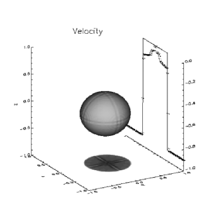
Figure 7: Three dimensional isosurfaces of density (top left), total velocity (top right), pressure (bottom left) and specific internal energy (bottom right) for the relativistic spherical shock reflection test problem (RSSR) at $t=2$. The inflow velocity for this case is $v_{in}=-0.9$. The intensity plots below each rendered surface show two-dimensional slices of the same quantity in the XY plane at at $z=0$. Finally, the numerical (diamonds) and analytic (solid line) solutions at $y,z=0$ are compared in the one dimensional plots projected on the YZ plane. The resolution adopted for this case is $101^{3}$ and integration has been carried with $CFL=0.4$.

Figure 7 shows the results for $v_{in}=-0.9$ on $101^{3}$ computational zones; the Courant number is $C_{a}=0.4$. The relative global errors (computed as in Aloy et al., 1999) for density, velocity and pressure are, respectively, $10.7\%$, $0.7\%$, $16.4\%$. Numerical symmetries (computed as $\max(\rho(x_{i},y_{j},0)-\rho(0,y_{k},z_{j})$) are retained to $10^{-7}$ for this case. From the same Figure we notice that our solver suffers from the wall-heating phenomenon, typical of such schemes.

We also investigated the ultra-relativistic regime by increasing the inflow velocity according to $v_{in}=\nu-1$, where $\nu=10^{-1},10^{-3},10^{-5},10^{-7}$, the latter corresponding to a Lorentz factor of $\gamma_{in}\approx 2236$. Following Aloy et al. (1999) we perform this set of simulations on $81^{3}$ zones. The relative global errors are given in Table 4.

4.4 Multi-dimensional Applications

Relativistic hydrodynamics is expected to play an important role in many phenomena typical in high energy astrophysics. In this Section we present the results of application of our new algorithm to the problem of propagation of relativistic jets. In the first problem we consider a highly supersonic pressure-matched light jet propagating in a constant density medium. In our second example we study the evolution of a light, high-Lorentz factor jet in a stratified medium, a situation frequently considered in the context of cosmological gamma-ray bursts.

4.4.1 Axisymmetric Jet

We consider the propagation of an axisymmetric relativistic jet in 2-D cylindrical coordinates. The computational domain covers the region $0<r<15$ and $0<z<45$ jet radii. At $t=0$ the jet is placed on the grid inside the region $z\leq 1$, $r\leq 1$ with velocity $v_{z}=0.995$ parallel to the symmetry axis and jet beam density $\rho_{b}=1$. The ambient medium has density $\rho_{m}=100$ and pressure is uniform everywhere, $p=0.005$.

We use the $TM$ equation of state, equation (96), which for the current conditions yields a relativistic beam Mach number of $\gamma v_{z}/(c_{s}\gamma_{c_{s}})\approx 110.5$ (corresponding to a classical Mach number $v_{b}/c_{s}\approx 11$). The computational domain is covered by $360\times 960$ equally spaced zones in the $\hat{\boldsymbol{n}}_{r}$ and $\hat{\boldsymbol{n}}_{z}$ direction respectively. At the symmetry axis we apply reflecting boundary conditions. Free outflow is allowed for at all other boundaries with the exception of the jet inlet ($z=0$, $r<1$) where $(\rho,\boldsymbol{v},p)$ are kept at their initial values. The integration is performed with $C_{a}=0.4$.

We follow the evolution until $t=80$ (in units of jet radius crossing time at the speed of light). By that time the jet has developed a rich and complex structure (Fig. 9). The morphology of the jet cocoon is determined by the interaction of the supersonic collimated beam (inside $r\lesssim 1$) with the shocked ambient gas. The beam is decelerated by the Mach disk and is terminated by the contact discontinuity where the beam material is deflected sideways feeding the cocoon. The interface between the jet backflowing material and the ambient shocked gas is Kelvin-Helmholtz unstable resulting in the formation of vortices and mixing. For the current conditions the jet cocoon shows a mix of turbulent regions close to the beam and relatively smooth outer sections traversed by a number of weak sound waves. The beam shows 3-4 internal shocks in its middle section and another strong internal shock about 10 jet radii behind the jet head.

Our results favorably compare to the previous study of Martí et al. (1997). Although in our simulation we do not use an ideal EoS, the equivalent adiabatic index, defined through equation (92) as $\Gamma_{eq}=(h-1)/(h-1-\Theta)$, always remains very close to $5/3$ making direct comparison with other studies possible. Specifically, our choice of parameters places the presented model between models $C2$ and $C3$ of Martí et al. (1997). Figure 8 shows the position of the jet head as a function of time. We find that during the early evolution ($t\lesssim 40$) the jet head velocity agrees very well with the one-dimensional theoretical estimate given by Martí et al. (1997). At later times, $40\lesssim t\lesssim 60$, the jet enters a deceleration stage after which ($t\gtrsim 60$) the velocity becomes again comparable with the theoretical prediction.

The propagation efficiency, defined as the ratio between the average head velocity and its one-dimensional estimate, is found to be $\approx 0.92$. This result is consistent with the previous results obtained for highly-supersonic light jets with large adiabatic index for which beam velocities tend to have propagation efficiency close to 1 (see Table 2 in Martí et al., 1997).

4.4.2 Gamma Ray Burst

We propose a simplified model for the propagation of a relativistic jet through a collapsing, non-rotating massive star. Such objects are believed to be sources of long-duration gamma ray bursts observed at cosmological distances (Frail et al., 2001; Woosley & MacFayden, 1999; Aloy et al., 2000). Our choice of parameters closely reflects that of model JB of Zhang et al. (2003).

We adopt spherical coordinates $(r,\theta)$. The domain has $320$ uniformly spaced zones between $1\leq r/r_{0}\leq 11$ and $500$ geometrically stretched zones in the range $11\leq r/r_{0}\leq 500$. Here $r_{0}=2\cdot 10^{8}$ cm is the inner grid boundary. The grid in the $\theta$ direction consists of $180$ uniformly-spaced zones for $0^{\circ}\leq\theta\leq 30^{\circ}$, while it is geometrically stretched with $100$ zones covering the region $30^{\circ}\leq\theta\leq 90^{\circ}$.

For the sake of simplicity, density and pressure distributions in the stellar progenitor are given by single power-laws,

$$\rho_{m}=\rho_{0}\left(\frac{r_{0}}{r}\right)^{a}\,,\quad p_{m}=p_{0}\left(\frac{r_{0}}{r}\right)^{b}\,,$$ (105)

while the velocity is zero everywhere. We adopted $a=1.77$, $b=2.6$, $\rho_{0}=10^{6}$ gr/cm³, and $p_{0}=8.33\cdot 10^{23}$ dyn/cm³ to match the progenitor model of Zhang et al. (2003). To account for gravity we included an external force corresponding to a $5M_{\odot}$ gravitational point mass placed at $r=0$. This is accounted for during the source step of our algorithm.

The jet is injected at $r=r_{0}$, $0\leq\theta\leq\theta_{0}$ where $\theta_{0}$ is the jet half-opening angle. The jet is characterized by its Lorentz factor $\gamma_{b}$, energy deposition rate (jet power)

$$\dot{E}_{b}=\rho_{b}\gamma_{b}(h_{b}\gamma_{b}-1)v_{b}2\pi r_{0}^{2}(1-\cos\theta_{0})\,,$$ (106)

and kinetic to total energy density ratio

$$f=\frac{\rho_{b}\gamma_{b}(\gamma_{b}-1)}{\rho_{b}\gamma_{b}(h_{b}\gamma_{b}-1)-p_{b}}\,,$$ (107)

where $\rho_{b}$, $h_{b}$ and $p_{b}$ are the proper density, specific enthalpy and pressure of the beam, respectively. Notice that the total energy density considered here does not include the rest mass energy. Equations (106) and (107) are used to express pressure and density as functions of the jet power, fractional kinetic energy density, Lorentz factor, and jet half-opening angle. For the present application we use $\dot{E}_{b}=10^{51}$ erg s^-1, $f=0.33$, $\gamma_{b}=50$ and $\theta_{0}=5^{\circ}$. The $TM$ equation of state is adopted and the CFL number is $C_{a}=0.6$. Reflecting boundary conditions are used at $\theta=0$ and $\theta=90^{\circ}$, while we allow for a free outflow at the outer grid boundary ($r/r_{0}=500$) and at the inner boundary outside the injection region. We follow the evolution until the jet has reached the outer boundary at $r=10^{11}$ cm.

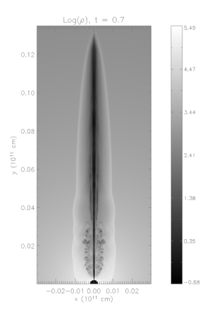
Figure 11: Density distribution at $t=0.7$ s (left panel) and $t=3.5$ s (right panel) for the gamma ray burst problem. The grid is unevenly spaced with a higher resolution close to the polar axis. The low density channel along the polar axis is evident at both times. The result can be compared to Zhang et al. (2003), Figure 2.

The results of our simulation are shown in Figure 11. During the early stages ($t\lesssim 1$ s, left panel in Fig. 11) the jet beam is quickly collimated by the high pressure of the near stellar environment, $p_{m}/p_{b}\approx 263.5$. By $t=3.5$ s (right panel in Fig. 11), the jet has cleared a low-density, high-velocity thin funnel along the polar axis and remains narrowly collimated with a very thin featureless cocoon. The latter property reflects the fact that ultra-relativistic jets are less prone to Kelvin-Helmholtz instabilities (Ferrari et al., 1978; Martí et al., 1997). This behavior is typical for supersonic light jets characterized by low Mach numbers ($M_{b}\approx 1.82$ and $\rho_{b}/\rho_{m}|_{r=r_{0}}\approx 1.85\cdot 10^{-5}$ for the present case). One should also be aware that our simulation includes a certain amount of numerical diffusion which limits the resolution of small scale structures in our model. This is specially true at large radii where the resolution of our mesh is coarser (the zone width increases geometrically with radius) and the geometry is diverging (spatial resolution decreases laterally).

Our results stay qualitative in agreement with the results of Zhang et al. (2003) with only minor differences. Specifically, the jet in our model propagates about 50% faster for $t<0.7$ s but reaches a similar distance by the final time ($t=3.5$ s). The morphological differences between the two models are small, with the current model having a slightly narrower beam and a less prominent cocoon. These discrepancies likely result from a combination of factors including differences of the numerical methods, initial conditions, and physics (we used simplified equation of state and neglect radiation effects). Overall, however, the evolution of the jet in both models is very similar.

5 CONCLUSIONS

We presented a high-resolution numerical scheme for special relativistic multidimensional hydrodynamics in general curvilinear coordinates. A finite volume, Godunov-type formulation is used, where volume averaged conserved quantities are evolved in time by solving Riemann problems at each time step. The solver takes into account non-vanishing tangential velocities at each zone interface and assumes that the two non-linear waves are shocks (i.e. “two-shock” approximation is used). This greatly reduces the computational cost and turns out to provide a reasonable approximation in the limit of weak rarefaction waves (as long as the time integration is done explicitly so that the time step is relatively small). The solution to the Riemann problem is found iteratively and a new method of incorporating a general EoS is presented.

We considered four different equations of state suitable for relativistic hydrodynamics. A novel simple analytic formulation for the relativistic perfect gas EoS has been presented. Our new equation of state recovers the exact solution (Synge, 1957) with accuracy better than 4%. This formulation is consistent with a special relativistic formulation of the kinetic theory of gases and shows the correct asymptotic behavior in the limit of very high and very low temperatures. Since our EoS is given by a simple analytic expression, the computational cost of the solution of the Riemann problem is significantly reduced.

Multidimensional integration is done with the fully coupled corner-transport upwind method (Colella, 1990; Saltzman, 1994; Miller & Colella, 2002). Preserving symmetries of the problem is often difficult especially when directionally split advection algorithm is used and may require applying special procedures (Aloy et al., 1999). Our choice of an unsplit integrator makes the presented method free of such problems and symmetries of the flow are perfectly preserved.

The calculation of the numerical fluxes requires solving 4 Riemann problems in two dimensions and 12 Riemann problems in three dimensions per cell per time step. This compares to 6 Riemann problems to be solved for the unsplit second-order Runge-Kutta schemes (in three dimensions) which in practice, however, usually require smaller time steps. Second-order accuracy in time is achieved by using characteristic projection operators.

Our implementation is verified in the case of strongly relativistic flows with Lorentz factor in excess of $2\cdot 10^{3}$. Purely one-dimensional test problems with non-vanishing tangential velocity are used to demonstrate the formal correctness of the method. The implementation is verified in two dimensions using a Riemann problem with two shocks and two contact discontinuities. Performance of the new method is illustrated using two astrophysical applications: a pressure-matched light relativistic jet with Mach number $\approx 11$ and $\Gamma\approx 10$ in 2-D cylindrical geometry and the propagation of a highly relativistic ($\Gamma>50$) jet through the stellar atmosphere in spherical geometry. The latter problem is motivated by studies of relativistic jets in collapsars (Zhang et al., 2003).

Appendix A ORTHOGONAL CURVILINEAR COORDINATES

In what follows we show how the geometrical source term $\boldsymbol{S}_{G}$ (eq. [30]) can be calculated for an arbitrary orthogonal system of coordinates. We also provide explicit expressions for the scale factors, face areas and zone volumes as required by the conservative finite volume formulation presented in §3. Expressions are given for the most commonly used coordinate systems: cartesian, cylindrical and spherical.

Consider the rank-two tensor, $\boldsymbol{T}=\sum_{a,b}T_{ab}\hat{\boldsymbol{n}}_{a}\hat{\boldsymbol{n}}_{b}$. The divergence of $\boldsymbol{T}$ is the vector

$$\nabla\cdot\boldsymbol{T}=\frac{1}{h_{1}h_{2}h_{3}}\sum_{d=1}^{3}\left(\frac{\partial(h_{2}h_{3}T_{1d})}{\partial x^{1}}+\frac{\partial(h_{1}h_{3}T_{2d})}{\partial x^{2}}+\frac{\partial(h_{1}h_{2}T_{3d})}{\partial x^{3}}\right)\hat{\boldsymbol{n}}_{d}+{\boldsymbol{S}_{G}}(\boldsymbol{T})\,,$$ (A1)

where ${\boldsymbol{S}_{G}}(\boldsymbol{T})$ is the source term contributed by those versors that do not have fixed orientation in space. The source term vector can be expressed as

$${\boldsymbol{S}_{G}}(\boldsymbol{T})=\sum_{d=1}^{3}\left(\frac{T_{1d}}{h_{1}}\frac{\partial\hat{\boldsymbol{n}}_{d}}{\partial x^{1}}+\frac{T_{2d}}{h_{2}}\frac{\partial\hat{\boldsymbol{n}}_{d}}{\partial x^{2}}+\frac{T_{3d}}{h_{3}}\frac{\partial\hat{\boldsymbol{n}}_{d}}{\partial x^{3}}\right)\,,$$ (A2)

with components

$$\hat{\boldsymbol{n}}_{d}\cdot{\boldsymbol{S}_{G}}(\boldsymbol{T})=\frac{1}{h_{d}}\sum_{a\neq d}\left(\frac{T_{da}}{h_{a}}\frac{\partial h_{d}}{\partial x^{a}}-T_{aa}\frac{\partial\log(h_{a})}{\partial x^{d}}\right)\,.$$ (A3)

The tensor $\boldsymbol{T}$ appears as the dyad $\boldsymbol{m}\boldsymbol{v}$ in equation (30).

First we consider Cartesian coordinates $(x^{1},x^{2},x^{3})=(x,y,z)$. The geometric scale factors are $h_{x}=h_{y}=h_{z}=1$ so that ${\boldsymbol{S}_{G}}(\boldsymbol{T})$ is identically zero. The cell volume is $\Delta\mathcal{V}_{ijk}=\Delta x_{i}\Delta y_{j}\Delta z_{k}$ and the surface areas of the six bounding cell faces are

$$A^{x}_{i\pm\frac{1}{2},j,k}=\Delta y_{j}\Delta z_{k}\,,\quad A^{y}_{i,j\pm\frac{1}{2},k}=\Delta x_{i}\Delta z_{k}\,,\quad A^{z}_{i,j,k\pm\frac{1}{2}}=\Delta x_{i}\Delta y_{j}\,.$$ (A4)

In cylindrical coordinates, $(x^{1},x^{2},x^{3})\equiv(r,\phi,z)$, the scale factors are

$$h_{r}=1\,,\quad h_{\phi}=r\,,\quad h_{z}=1\,.$$ (A5)

while the cell volume is

$$\Delta\mathcal{V}_{i,j,k}\equiv\int_{r_{i-\frac{1}{2}}}^{r_{i+\frac{1}{2}}}\int_{\phi_{j-\frac{1}{2}}}^{\phi_{j+\frac{1}{2}}}\int_{z_{k-\frac{1}{2}}}^{z_{k+\frac{1}{2}}}r\,drdzd\phi=\left(\frac{r^{2}_{i+\frac{1}{2}}-r^{2}_{i-\frac{1}{2}}}{2}\right)\Delta\phi_{j}\Delta z_{k}\,.$$ (A6)

The areas of cell faces are

$$A^{r}_{i\pm\frac{1}{2},j,k}=r_{i\pm\frac{1}{2}}\Delta\phi_{j}\Delta z_{k}\,,\quad A^{\phi}_{i,j\pm\frac{1}{2},k}=\Delta r_{i}\Delta z_{k}\,,\quad A^{z}_{i,j,k\pm\frac{1}{2}}=\left(\frac{r^{2}_{i+\frac{1}{2}}-r^{2}_{i-\frac{1}{2}}}{2}\right)\Delta\phi_{j}\,,$$ (A7)

and the geometrical source vector is

$${\boldsymbol{S}_{G}}(\boldsymbol{m}\boldsymbol{v})=-\frac{m_{\phi}v_{\phi}}{r}\hat{\boldsymbol{n}}_{r}+\frac{m_{\phi}v_{r}}{r}\hat{\boldsymbol{n}}_{\phi}\,.$$ (A8)

In spherical coordinates, $(x^{1},x^{2},x^{3})\equiv(r,\theta,\phi)$, the scale factors are

$$h_{r}=1\,,\quad h_{\theta}=r\,,\quad h_{\phi}=r\sin\theta\,,$$ (A9)

the cell volume is

$$\Delta\mathcal{V}_{i,j,k}\equiv\int_{r_{i-\frac{1}{2}}}^{r_{i+\frac{1}{2}}}\int_{\theta_{j-\frac{1}{2}}}^{\theta_{j+\frac{1}{2}}}\int_{\phi_{k-\frac{1}{2}}}^{\phi_{k+\frac{1}{2}}}r^{2}\sin\theta\,drd\theta d\phi=\left(\frac{r_{i+\frac{1}{2}}^{3}-r_{i-\frac{1}{2}}^{3}}{3}\right)\left(\cos\theta_{j-\frac{1}{2}}-\cos\theta_{j+\frac{1}{2}}\right)\Delta\phi_{k}\,,$$ (A10)

and surface areas are

$$A^{r}_{i\pm\frac{1}{2},j,k}=r^{2}_{i\pm\frac{1}{2}}\left(\cos\theta_{j-\frac{1}{2}}-\cos\theta_{j+\frac{1}{2}}\right)\Delta\phi_{k}\,,$$ (A11)

$$A^{\theta}_{i,j\pm\frac{1}{2},k}=\left(\frac{r^{2}_{i+\frac{1}{2}}-r^{2}_{i-\frac{1}{2}}}{2}\right)\sin\theta_{j\pm\frac{1}{2}}\Delta\phi_{k}\,,$$ (A12)

$$A^{\phi}_{i,j,k\pm\frac{1}{2}}=\left(\frac{r^{2}_{i+\frac{1}{2}}-r^{2}_{i-\frac{1}{2}}}{2}\right)\Delta\theta_{j}\,.$$ (A13)

In this case the geometrical source term is

$${\boldsymbol{S}_{G}}(\boldsymbol{m}\boldsymbol{v})=\left(-\frac{m_{\theta}v_{\theta}+m_{\phi}v_{\phi}}{r}\right)\hat{\boldsymbol{n}}_{r}+\left(\frac{m_{\theta}v_{r}-\cot\theta m_{\phi}v_{\phi}}{r}\right)\hat{\boldsymbol{n}}_{\theta}+\left(\frac{m_{\phi}v_{r}+\cot\theta m_{\phi}v_{\theta}}{r}\right)\hat{\boldsymbol{n}}_{\phi}\,.$$ (A14)

Appendix B RECONSTRUCTION PROCEDURE

In our parabolic reconstruction procedure we closely follow the prescription of CW84 with only minor modifications. The contact steepening algorithm, specific to PPM, has been used only for one-dimensional tests and will not be reported here (for details see Martí & Müller, 1996). We also note that, as it was pointed out by CW84, in order to preserve accuracy of the scheme the interpolation should be formally done using the conservative variables. Reconstruction based on primitive variables offers, however, some advantages (preserves pressure positivity and in case of relativistic hydrodynamics allows to satisfy kinematical and thermodynamic constraints) and is our method of choice.

Let $\bar{q}$ be the volume-average of some quantity $q$, $Q(\xi)=\int^{\xi}q(\xi^{\prime})\,d\xi^{\prime}$ its integral, where $\xi$ is a generic volume coordinate. Here we adopt the implied notation $q\leftrightarrow q_{i,j,k}$ whenever $i$, $j$ or $k$ are not present (the same convention is adopted also for other three-dimensional quantities). The reconstruction process begins with interpolating a quartic polynomial through $Q_{i\pm 2+\frac{1}{2}}$,$Q_{i\pm 1+\frac{1}{2}}$,$Q_{i+\frac{1}{2}}$. This polynomial is used to calculate the single-valued estimate

$$q_{i+\frac{1}{2}}=\left.\frac{dQ(\xi)}{d\xi}\right|_{\xi=\xi_{i+\frac{1}{2}}}\,,$$ (B1)

at the zone interfaces. The explicit result of this construction is (CW84)

$$q_{i+\frac{1}{2}}=\bar{q}_{i}+a_{i}\left(\bar{q}_{i+1}-\bar{q}_{i}\right)+b_{i}\overline{\delta q}_{i}-c_{i}\overline{\delta q}_{i+1}\,,$$ (B2)

with

$$a_{i}=\frac{\Delta\xi_{i}}{\Delta\xi_{i}+\Delta\xi_{i+1}}+\frac{2(\Delta\xi_{i+1}c_{i}-\Delta\xi_{i}b_{i})}{\Delta\xi_{i}+\Delta\xi_{i+1}}\,,$$ (B3)

$$b_{i}=\left(\frac{\Delta\xi_{i+1}}{\sum_{k=-1}^{k=2}\Delta\xi_{i+k}}\right)\frac{\Delta\xi_{i+1}+\Delta\xi_{i+2}}{\Delta\xi_{i}+2\Delta\xi_{i+1}}\,,\quad c_{i}=\left(\frac{\Delta\xi_{i}}{\sum_{k=-1}^{k=2}\Delta\xi_{i+k}}\right)\frac{\Delta\xi_{i-1}+\Delta\xi_{i}}{2\Delta\xi_{i}+\Delta\xi_{i+1}}\,.$$ (B4)

Monotonicity is enforced by limiting $q_{i+\frac{1}{2}}$ to lie between $\bar{q}_{i}$ and $\bar{q}_{i+1}$. This is achieved by using the limiter (VanLeer, 1997)

$$\overline{\delta q}_{i}=\left\{\begin{array}[]{ll}\min(|\delta q_{i}|,2|\bar{q}_{i}-\bar{q}_{i-1}|,2|\bar{q}_{i}-\bar{q}_{i+1}|)\textrm{sgn}(\delta q_{i})&\textrm{if}\;(\bar{q}_{i+1}-\bar{q}_{i})(\bar{q}_{i}-\bar{q}_{i-1})>0\,,\\ \vskip 6.0pt plus 2.0pt minus 2.0pt\cr 0&\textrm{otherwise}\,,\end{array}\right.$$ (B5)

where

$$\delta q_{i}=\frac{\Delta\xi_{i}}{\Delta\xi_{i-1}+\Delta\xi_{i}+\Delta\xi_{i+1}}\left[\frac{2\Delta\xi_{i-1}+\Delta\xi_{i}}{\Delta\xi_{i+1}+\Delta\xi_{i}}\left(\bar{q}_{i+1}-\bar{q}_{i}\right)+\frac{2\Delta\xi_{i+1}+\Delta\xi_{i}}{\Delta\xi_{i-1}+\Delta\xi_{i}}\left(\bar{q}_{i}-\bar{q}_{i-1}\right)\right]\,,$$ (B6)

is the average slope. At the end of this step we initialize

$$q_{i+\frac{1}{2},L}=q_{i+\frac{1}{2},R}=q_{i+\frac{1}{2}}\,,$$ (B7)

where $q_{i+\frac{1}{2},L}$ and $q_{i+\frac{1}{2},R}$ are the left and right limiting values of $q$ at the zone’s right interface.

Next, we constrain the interface values for zone $i,j,k$ to lie within the extreme values found among all neighboring cells (Barth, 1995). Construction for $q_{i+\frac{1}{2},L}$ (identical procedure is followed to limit $q_{i-\frac{1}{2},R}$) proceeds as follows. Let $\hat{q}^{\max}$ and $\hat{q}^{\min}$ be, respectively, the maximum and minimum value of $\bar{q}_{I,J,K}$ for $I=i-1,i,i+1$, $J=j-1,j,j+1$, $K=k-1,k,k+1$. Then

$$q_{i+\frac{1}{2},L}=\max\left(\hat{q}^{\min},\min\left(\hat{q}^{\max},q_{i+\frac{1}{2},L}\right)\right)\,.$$ (B8)

Notice that in two and three dimensions there is a total of 9 and 27 zones involved in the limiting step.

In the next step we limit the parabolic distribution of $q$ to ensure that its profile remains monotonic in each cell. A first case when monotonicity can be violated is when $\bar{q}$ is a local maximum or minimum. In this case we revert to first order interpolation:

$$q_{i+\frac{1}{2},L}\;\rightarrow\;\bar{q}\qquad\textrm{if}\quad(q_{i-\frac{1}{2},R}-\bar{q})(\bar{q}-q_{i+\frac{1}{2},L})\leq 0\,.$$ (B9)

Monotonicity can also be violated if the parabolic distribution (54) has an extremum inside the zone. In this case one of the interface values is adjusted so that the parabolic profile has an extremum at the other interface. The modified distribution also has to preserve the correct zone-average value. The final result is:

$$q_{i-\frac{1}{2},R}\;\rightarrow\;3\bar{q}-2q_{i+\frac{1}{2},L}\qquad\textrm{if}\quad\left(q_{i+\frac{1}{2},L}-q_{i-\frac{1}{2},R}\right)\left(\bar{q}-\frac{q_{i+\frac{1}{2},L}+q_{i-\frac{1}{2},R}}{2}\right)>\frac{\left(q_{i+\frac{1}{2},L}-q_{i-\frac{1}{2},R}\right)^{2}}{6}\,,$$ (B10)

$$q_{i+\frac{1}{2},L}\;\rightarrow\;3\bar{q}-2q_{i-\frac{1}{2},R}\qquad\textrm{if}\quad\left(q_{i+\frac{1}{2},L}-q_{i-\frac{1}{2},R}\right)\left(\bar{q}-\frac{q_{i+\frac{1}{2},L}+q_{i-\frac{1}{2},R}}{2}\right)<-\frac{\left(q_{i+\frac{1}{2},L}-q_{i-\frac{1}{2},R}\right)^{2}}{6}\,.$$ (B11)

It should also be mentioned that the reconstruction algorithm may occasionally fail to respect the condition $v_{1}^{2}+v_{2}^{2}+v_{3}^{2}<1$. To prevent this from happening, interpolation of the velocity components reverts to first order whenever the total velocity exceeds the bounds provided by the neighboring cells, in a way similar to equation (B8).

B.1 Dissipation Algorithm

Interpolation profiles are modified in presence of strong shocks to prevent unphysical oscillations. This is achieved by the flattening algorithm in which the interface values are modified as

$$q_{i+\frac{1}{2},L}=\chi q_{i+\frac{1}{2},L}+(1-\chi)\bar{q}\,,$$ (B12)

$$q_{i-\frac{1}{2},R}=\chi q_{i-\frac{1}{2},R}+(1-\chi)\bar{q}\,,$$ (B13)

where $\chi$ is a multi-dimensional flattening parameter, $0\leq\chi\leq 1$. Note that for $\chi=0$ the accuracy of the method reduces to first order. The flattening parameter is computed as (Miller & Colella, 2001, 2002)

$$\chi=\min_{I,J,K}\left(\tilde{\chi}_{1,I,j,k},\tilde{\chi}_{2,i,J,k},\tilde{\chi}_{3,i,j,K}\right)\,,$$ (B14)

where the minimum is taken over all $I,J,K$ in the range $i-1\leq I\leq i+1$, $j-1\leq J\leq j+1$, $k-1\leq K\leq k+1$. The coefficients $\tilde{\chi}_{1}$, $\tilde{\chi}_{2}$ and $\tilde{\chi}_{3}$ are one-dimensional. In what follows we describe the procedure only for $\tilde{\chi}_{1}$; the remaining two values are calculated in the same way. First, we introduce a measure of the shock width

$$\beta_{1}=\frac{|p_{i+1}-p_{i+1}|}{|p_{i+2}-p_{i+2}|}\,,$$ (B15)

and shock strength

$$Z_{1}=\frac{|p_{i+1}-p_{i-1}|}{\min(p_{i-1},p_{i+1})}\,.$$ (B16)

Next we define

$$\tilde{\chi}^{min}_{1}=\max\left(0,\min\left(1,\frac{\beta^{max}-\beta_{1}}{\beta^{max}-\beta^{min}}\right)\right)\,,$$ (B17)

so that flattening is not applied for $\beta<\beta^{min}$. The one-dimensional flattening parameter is then restricted only to the regions where the flow undergoes compression and its value depends on the shock strength:

$$\tilde{\chi}_{1}=\left\{\begin{array}[]{ll}\displaystyle\max\left(\tilde{\chi}^{\min}_{1},\min\left(1,\frac{Z^{max}-Z_{1}}{Z^{max}-Z^{min}}\right)\right)&\qquad\textrm{if}\quad v_{1,i+1}<v_{1,i}\,,\\ \vskip 6.0pt plus 2.0pt minus 2.0pt\cr 1&\qquad\textrm{otherwise}\,.\\ \end{array}\right.$$ (B18)

For the present study we follow recommendation of Miller & Colella (2002) and adopt $\beta^{max}=0.85$, $\beta^{min}=0.75$, $Z^{max}=0.75$, $Z^{min}=0.25$.

Slope flattening is combined with the introduction of an explicit diffusive flux, in order to further reduce spurious oscillations behind strong shocks. To this purpose, the numerical fluxes (eq. [36]) in the final conservative update are augmented as

$$\boldsymbol{F}_{i+\frac{1}{2}}\;\rightarrow\;\boldsymbol{F}_{i+\frac{1}{2}}+k_{\nu}\left(\boldsymbol{U}-\boldsymbol{U}_{i+1}\right)\,.$$ (B19)

Here

$$k_{\nu}=\alpha\max\left(-\mathcal{D}_{i+\frac{1}{2}},0\right)\,,$$ (B20)

where $\alpha$ is typically set to $0.1$. $\mathcal{D}_{i+\frac{1}{2}}$ is a measure of the convergence of the flow at the zone interface $i+\frac{1}{2}$. In cartesian coordinates with a uniform zone spacing ($\Delta x=\Delta y=\Delta z$), $\mathcal{D}_{i+\frac{1}{2}}$ is a discrete undivided difference approximation to the multidimensional divergence of $\boldsymbol{v}$. In order to compute $\mathcal{D}_{i+\frac{1}{2}}$, we define a measure of the convergence of the flow at the cell corners as

$$\begin{array}[]{cl}\mathcal{D}_{i+\frac{1}{2},j+\frac{1}{2},k+\frac{1}{2}}=\displaystyle\frac{1}{4}&\displaystyle\left[\sum_{J=j,j+1\atop K=k,k+1}\left(v_{1,i+1,J,K}-v_{1,i,J,K}\right)\right.\displaystyle+\left.\sum_{I=i,i+1\atop K=k,k+1}\left(v_{2,I,j+1,K}-v_{2,I,j,K}\right)\right.\\ &\displaystyle+\left.\sum_{I=i,i+1\atop J=j,j+1}\left(v_{3,I,J,k+1}-v_{3,I,I,k}\right)\right]\,,\end{array}$$ (B21)

so that $\mathcal{D}_{i+\frac{1}{2}}$ is obtained by a simple average procedure

$$\mathcal{D}_{i+\frac{1}{2}}=\frac{1}{4}\left(\mathcal{D}_{i+\frac{1}{2},j+\frac{1}{2},k+\frac{1}{2}}+\mathcal{D}_{i+\frac{1}{2},j-\frac{1}{2},k+\frac{1}{2}}+\mathcal{D}_{i+\frac{1}{2},j+\frac{1}{2},k-\frac{1}{2}}+\mathcal{D}_{i+\frac{1}{2},j-\frac{1}{2},k-\frac{1}{2}}\right)\,.$$ (B22)

Figure 1: Solution of the Riemann problem in the $\xi-t$ plane. The discontinuity between the two states $L$ and $R$ initially located at $\xi=0$ decays into a set of three waves. The emerging pattern divides the $\xi-t$ plane into the four distinct regions labeled by $L,L^{*},R^{*},R$. A contact discontinuity separates state $L^{*}$ from state $R^{*}$, while the $R^{*}R$ and $LL^{*}$ waves can be either shocks or rarefactions (in this picture the $LL^{*}$ and $R^{*}R$ wave are, respectively, a rarefaction wave and a shock).

Figure 2: Graphical solution in the $v-p$ plane of $v(p,R)$ and $v(p,L)$; the intersection between the two curves is the solution to the Riemann problem in the two-shock approximation.

Figure 3: Plots of the function $\Gamma_{r}(\Theta)$ vs. temperature logarithm ($\log\Theta$, $\Theta=p\tau$) for the four different EoS discussed in the text. The $TM$ EoS (solid line) marks the lower boundary of Taub’s inequality (93). The relativistic perfect gas EoS ($RP$, eq. [94]) always lies above the boundary line, and therefore satisfies Taub’s inequality for every $\Theta$. The interpolated EoS ($IP$, eq. [95]) approaches the correct limit only at high temperatures. The horizontal lines correspond to the ideal EoS plotted for $\Gamma=5/3$ and $\Gamma=4/3$, but only the second one satisfies Taub’s inequality for $0\leq\theta<\infty$.

Figure 4: The numerical solution (given by the symbols) compared to the exact analytical solution (solid line) for the relativistic shock tube (P1 in the text), at t=0.36 is shown. The wave structure is well described by our numerical scheme: both the shock and the contact wave are smeared out on $4-5$ and $2-3$ zones, respectively, in the density profile (asterisk marks). For this test problem $400$ equally spaced zones were used and $C_{a}=0.9$.

Figure 5: Relativistic shock tube (P2): analytical solution (solid lines) and numerical solutions on 400 zones are shown at $t=0.4$; from left to right $v_{yR}=0,0.9,0.99$, from top to bottom $v_{yL}=0,0.9,0.99$.

Figure 6: Initial condition for the 2-D riemann problem (on the left) and solution at t= 0.4 (right). In order to have simple shocks at the $(2\leftrightarrow 1)$, $(4\leftrightarrow 1)$ interfaces, the value of density and pressure in region $1$ are $\rho_{1}=5.477875\cdot 10^{-3}$, $p_{1}=2.762987\cdot 10^{-3}$.

Figure 8: Distance traveled by the jet head as a function of time. The triangles show the position of the head in our simulation at different times, while the solid line represents the relativistic one-dimensional estimate.

Figure 9: Density distribution, in logarithmic scale, for the axisymmetric relativistic jet at $t=80$. The jet is initially in pressure equilibrium with the ambient medium, which is $100$ times denser than the jet; the initial velocity is $v_{z}=0.995$. The resolution is 24 zones per beam radius.

Figure 10: Lorentz factor for the gamma ray burst problem at $t=3.5$ s. The reverse shock is located at $\log r\approx 8.9$.

Table 1: Expressions for the different EoS, square of sound speed and solutions to the Taub adiabat for the four different cases presented in the text; the coefficients $a$, $b$ and $c$ for the $ID$ and $TM$ EoS are given by equations (98) and (99). The $*$ case has to be solved numerically.

EoS	$h(\Theta)$	$c_{s}^{2}$	Taub adiabat
ID	$\displaystyle 1+\Gamma_{r}\Theta$	$\displaystyle\frac{\Gamma\Theta}{h}$	$\displaystyle h=\frac{-b+\sqrt{b^{2}-4ac}}{2a}$
RP	$\displaystyle\frac{K_{3}(1/\Theta)}{K_{2}(1/\Theta)}$	$\displaystyle\frac{\Theta}{h}\frac{1+5h\Theta-h^{2}}{1+5h\Theta-h^{2}-\Theta^{2}}$	*
IP	$\displaystyle 2\Theta+\sqrt{4\Theta^{2}+1}$	$\displaystyle\frac{2\Theta}{h+2\Theta}$	$\displaystyle h^{2}=h_{S}^{2}+\frac{4h_{S}\tau_{S}[p^{2}]}{3p+p_{S}}$
TM	$\displaystyle\frac{5}{2}\Theta+\sqrt{\frac{9}{4}\Theta^{2}+1}$	$\displaystyle\frac{\Theta}{3h}\frac{5h-8\Theta}{h-\Theta}$	$\displaystyle[h\tau]=\frac{2c}{|b|+\sqrt{b^{2}-4ac}}$

Table 2: Expressions for the mass flux $j$, and derivative $d(h\tau)/dp$ for the four different EoS presented in the text; here $w\equiv h\tau$. Notice that for all but the RP case, the expressions for $j^{2}$ is numerically well behaved for $[p]\to 0$.

EoS	$j^{2}$	$d(h\tau)/dp$
ID	$\displaystyle\frac{\Gamma_{r}p}{\Gamma_{r}w_{S}+(w+w_{S})\left(\frac{1}{h+h_{S}}-1\right)}$	$\displaystyle\frac{w+w_{S}-\frac{2h}{2h-1}\Gamma_{r}w}{\frac{2h}{2h-1}\Gamma_{r}p-[p]}$
RP	$\displaystyle-\frac{pp_{S}[p]}{p_{S}[h\Theta]-h_{S}\Theta_{S}[p]}$	$\displaystyle\frac{(w+w_{S})(h-\dot{h}\Theta-2h\dot{h}w)}{2\dot{h}hp-[p](h-\dot{h}\Theta)}$
IP	$\displaystyle\frac{4p}{3w_{S}-w}$	$\displaystyle\frac{w_{S}-3w}{3p+p_{S}}$
TM	$\displaystyle\frac{|b|+\sqrt{b^{2}-4ac}}{2w_{S}(h^{2}_{S}+2w_{S}p+2)}$	$\displaystyle\frac{w(3h^{2}-3h\Theta+1)-w_{S}(2h^{2}-1-5h\Theta)}{1+[p](1+5h\Theta-2h^{2})}$

Table 3: Discrete L-1 norms of the conserved quantities for the shock tube problem (P1).

$\Delta x^{-1}$	$\|\epsilon_{D}\|_{1}$	$\|\epsilon_{m}\|_{1}$	$\|\epsilon_{E}\|_{1}$
50	$0.1620$	$0.2160$	$0.1560$
100	$0.0920$	$0.1420$	$0.1000$
200	$0.0505$	$0.0792$	$0.0558$
400	$0.0298$	$0.0436$	$0.0319$
800	$0.0118$	$0.0264$	$0.0206$
1600	$0.0115$	$0.0149$	$0.0126$

Note. — Errors are computed according to $\|\epsilon_{q}\|_{1}=\sum_{i}\Delta x|q_{i}-Q(x_{i})|$ (as in Martí & Müller (1996)), where $q$ is one of $D$, $m$, $E$, and $Q(x_{i})$ is the exact solution at $x=x_{i}$.

Table 4: Relative global errors (computed as in Aloy et al., 1999) for the Relativistic Spherical Shock Reflection (RSSR) test problem for different inflow velocities at $t=2$. Computations have been performed on a $81^{3}$ grid.

$\nu$	$\gamma$	$\|\epsilon_{\rho}\|_{1}$	$\|\epsilon_{v}\|_{1}$	$\|\epsilon_{p}\|_{1}$
$10^{-1}$	$2.29$	$0.18$	$0.01$	$0.29$
$10^{-3}$	$22.37$	$0.20$	$0.03$	$0.17$
$10^{-5}$	$223.6$	$0.26$	$0.04$	$0.20$
$10^{-7}$	$2236.1$	$0.21$	$0.04$	$0.24$

Note. — The inflow velocity is given by $v_{in}=\nu-1$. The corresponding Lorentz factor is given in the second column. The first two cases have been run with CFL = $0.4$, while CFL = $0.1$ has been used for the last two cases.

References

• Ackermann et al. (2001) Ackermann, K. H., et al. 2001, PRL, 86, 402
• Aloy et al. (1999) Aloy, M. A., Ibáñez, J. M. & Martí, J. M. 1999, ApJS, 122, 151
• Aloy et al. (2000) Aloy, M. A., Müller, E., Ibáñez, J. M., Martí, J. M. & MacFadyen, A. 2000, ApJ, 531, L119
• Aloy et al. (2003) Aloy, M. A., et al. 2003, ApJ, 585, L109
• Anile (1989) Anile, A. M. 1989, Relativistic Fluids and Magneto-fluids (Cambridge: Cambridge University Press), 55
• Balsara (1994) Balsara, D. S. 1994, J. Comput. Phys., 114, 284
• Barth (1995) Barth, T. J. 1995, Aspects of Unstructured Grids and Finite-Volume Solvers for Euler and Navier-Stokes Equations, VKI/NASA/AGARD Special Course on Unstructured Grid Methods for Advection Dominated Flows (AGARD Publ. R-787) (Belgium: Von Karmen Inst. for Fluid Dynamics)
• Begelman et al. (1984) Begelman, M. C., Blandford, R. D. & Rees, M. J. 1984, Rev. Mod. Phys., 56, 255
• Blondin & Lufkin (1993) Blondin, J. M. & Lufkin, E. A. 1993, ApJS, 88, 589
• Bogovalov et al. (2005) Bogovalov, S. V., et al. 2005, MNRAS, 358, 705
• Calder et al. (2002) Calder, A. C., et al. 2002, ApJS, 143, 201
• Colella (1982) Colella, P. 1982, SIAM J. Sci. Stat. Comput., 3, 76
• Colella & Woodward (1984) Colella, P. & Woodward, P. R. 1984, J. Comput. Phys., 54, 174
• Colella (1985) Colella, P. 1985, SIAM J. Sci. Stat. Comput., 6, 104
• Colella & Glaz (1985) Colella, P. & Glaz, H.M. 1985, J. Comput. Phys., 59, 264
• Colella (1990) Colella, P. 1990, J. Comput. Phys., 87, 171
• Courant et al. (1928) Courant, R., Friedrichs, K. O. & Lewy, H. 1928, Math. Ann., 100, 32
• Dai & Woodward (1997) Dai, W. & Woodward, P. R. 1997, SIAM J. Sci. Comput., 18, 982
• Del Zanna & Bucciantini (2002) Del Zanna, L. & Bucciantini, N. 2002, A&A, 390, 1177
• Del Zanna et al. (2004) Del Zanna, L., Amato, E. & Bucciantini, N. 2004, A&A, 421, 1063
• Dolezal & Wong (1995) Dolezal, A. & Wong, S. M. 1995, J. Comput. Phys., 120, 266
• Donat et al. (1998) Donat, R., Font, J. A., Ibáñez, J. M. & Marquina, A. 1998, J. Comput. Phys., 146, 58
• Falle & Komissarov (1996) Falle, S. A. E. G & Komissarov, S. S. 1996, MNRAS, 278, 586
• Ferrari et al. (1978) Ferrari, A., Trussoni, E. & Zaninetti, L. 1978, A&A, 64, 43
• Frail et al. (2001) Frail, D. A., et al. 2001, ApJ, 562, L55
• Koide et al. (1999) Koide, S., Shibata, K. & Sakai, J. 1999, ApJ, ApJ, 522, 727
• Lax & Liu (1998) Lax, P. D. & Liu, X.-D. 1998, SIAM J. Sci. Comput., 19, 319
• Landau & Lifshitz (1959) Landau, L. D. & Lifshitz, E. M. 1959, Fluid Mechanics (New York: Pergamon)
• Marquina et al. (1992) Marquina, A., Martí, J.M., Ibáñez, J. M., Miralles, J. A. & Donat, R. 1992, A&A, 258, 566
• Martí & Müller (1994) Martí, J. M. & Müller, E. 1994, J. Fluid Mech., 258, 317
• Martí & Müller (1996) Martí, J. M. & Müller, E. 1996, J. Comput. Phys., 123, 1
• Martí et al. (1997) Martí, J. M., Müller, E., Font, J. A., Ibanez, J. M. A. & Marquina, A. 1997, ApJ, 479, 151
• Martí & Müller (2003) Martí, J. M. & Müller, E. 2003, Living Reviews in Relativity, 6, 7
• Meier et al. (2001) Meier, D. L., Koide, S. & Uchida, Y. 2001, Science, 291, 84
• Miller & Colella (2001) Miller, G. H. & Colella, P. 2001, J. Comput. Phys., 167, 131
• Miller & Colella (2002) Miller, G. H. & Colella, P. 2002, J. Comput. Phys., 183, 26
• Mizuno et al. (2004) Mizuno, Y., et al. 2004, ApJ, 615, 389
• Molnar & Huovinen (2004) Molnar, D. & Huovinen, P. 2004, Phys. Rev. Lett., 94, 012302
• Morita et al. (2002) Morita, K., Muroya, S., Nonaka, C. & Hirano, T. 2004, Phys. Rev. C, 66, 054904
• Norman & Winkler (1986) Norman, M. L. & Winkler, K.-H. 1986, in Astrophysical Radiation Hydrodynamics, ed. K.-H. Winkler & M. Norman (Dordrecht: Kluwer), 449
• Pons et al. (2000) Pons, J.A., Martí, J.M. & Müller, E. 2000, J. Fluid Mech., 42, 125
• Rezzolla et al. (2003) Rezzolla, L., Zanotti, O., Pons, J.A., 2003, J. Fluid Mech., 479, 199
• Saltzman (1994) Saltzman, J. 1994, J. Comput. Phys., 115, 153
• Schulz et al. (1993) Schulz-Rinne, C. W., Collins, J. P. & Glaz, H. M. 1993, SIAM J. Sci. Comp., 14, 1394
• Sokolov et al. (2001) Sokolov, I. V., Zhang, H.-M. & Sakai, J. I. 2001, J. Comput. Phys., 172, 209
• Strang (1968) Strang, G., 1968, SIAM J. Num. Anal., 5, 506
• Synge (1957) Synge, J. L. 1957, The relativistic Gas, North-Holland Publishing Company
• Taub (1948) Taub, A. H. 1948, Physical Review, 74, 328
• Toro (1997) Toro, E. F. 1997, Riemann Solvers and Numerical Methods for Fluid Dynamics, Springer-Verlag, Berlin
• VanLeer (1997) VanLeer, B. 1997, J. Comput. Phys., 135, 229
• Weinberg (1972) Weinberg, S. 1972, Gravitation and Cosmology, (New York: Wiley)
• Wilson (1972) Wilson, J. R. 1972, A&A, 173, 431
• Woodward & Colella (1984) Woodward, P. R. & Colella, P. 1984, J. Comput. Phys., 54, 115
• Woosley & MacFayden (1999) Woosley, S. E. & MacFayden, A. I. 1999, A&A, 138, 499
• Zhang et al. (2003) Zhang, W., Woosley, S. E. & MacFayden, A. I. 2003, ApJ, 586, 356
Refer to caption