Global MHD Modelling of the ISM - From large towards small scale turbulence

Abstract

Dealing numerically with the turbulent nature and non-linearity of the physical processes involved in the ISM requires the use of sophisticated numerical schemes coupled to HD and MHD mathematical models. SNe are the main drivers of the interstellar turbulence by transferring kinetic energy into the system. This energy is dissipated by shocks (which is more efficient) and by molecular viscosity. We carried out adaptive mesh refinement simulations (with a finest resolution of 0.625 pc) of the turbulent ISM embedded in a magnetic field with mean field components of 2 and 3 $\mu$G. The time scale of our run was 400 Myr, sufficiently long to avoid memory effects of the initial setup, and to allow for a global dynamical equilibrium to be reached in case of a constant energy input rate. It is found that the longitudinal and transverse turbulent length scales have a time averaged (over a period of 50 Myr) ratio of 0.52-0.6, almost similar to the one expected for isotropic homogeneous turbulence. The mean characteristic size of the larger eddies is found to be $\sim 75$ pc in both runs. In order to check the simulations against observations, we monitored the Ovi and Hi column densities within a superbubble created by the explosions of 19 SNe having masses and velocities of the stars that exploded in vicinity of the Sun generating the Local Bubble. The model reproduces the FUSE absorption measurements towards 25 white dwarfs of the Ovi column density as function of distance and of N(Hi) . In particular for lines of sight with lengths smaller than 120 pc it is found that there is no correlation between N(Ovi) and N(Hi) .

1 Introduction

The Reynolds number of the ISM is of the order of $10^{6}$ or even higher. Thus, the ISM is a turbulent medium that is regularly stirred by shock waves generated in supernova explosions. At least $10\%$ of energy from SN blast waves is injected into the interstellar gas (Thornton et al. 1998; however, for higher efficiencies see Avillez & Breitschwerdt 2005c). The energy injected into turbulence at the largest scale is transferred to smaller and smaller eddies until it reaches the Kolmogorov inner scale of the order of $10^{-3}$ pc, or even lower.

The interstellar turbulence, which is mainly due to shear flows of large scale streams and its associated increase of vorticity, decays without constant energy supply. Attempts have been made to understand the time scales of the turbulence decay within molecular clouds and it was found that the presence of magnetic fields would only delay this decay (Mac Low et al. 1998). These studies use a computational domain having the size of the turbulence outer scale (the scale at which energy is injected). However, although molecular clouds can have sizes of a few tens of parsecs, they are embedded in a large scale interstellar medium (ISM) that is swept up by shock waves from SNe, driving large scale streams that eventually generate shock compressed layers leading to the formation of molecular clouds. In addition, the occupation fraction of the hot gas in the Galactic disk is low (some 20%; Avillez & Breitschwerdt 2004, 2005a) because there are kpc-scale flows escaping into the thick disk or into the halo through chimneys. These flows enter the disk-halo-disk cycle becoming later a source of turbulence in the disk as the Hi clouds, generated in the fountain, strike the disk and enhance the vorticity.

Modelling the ISM in a self-consistent way requires an approach, that takes into account the relevant turbulent scales, which cover several orders of magnitude as well as the disk-halo-circulation. This is a difficult task that requires the use of sophisticated numerical codes, adequate computing power, and precision input data by observations. Only since very recently, by the rapid evolution of telescope and detector technology, as well as the availability of large numbers of parallel processors, we are in the fortunate situation to follow in detail the evolution of the ISM on the global scale taking into account the disk-halo-disk circulation in three dimensions.

The plan of the present paper is as follows. In Section 2 a brief overview of the developments carried out in the 3D supernova-driven ISM model of Avillez (2000) (in order to provide a self-consistent picture of the ISM) is presented. Some results on turbulence scales and tests to the present model are discussed in Sections 3 and 4, respectively. In Section 5 a few final remarks are presented.

2 Modelling of a Supernova-driven ISM

The supernova-driven model coupled to a 3D magneto-hydrodynamical block mesh refinement scheme used to study the properties of the ISM in general (e.g., Avillez & Berry 2001; Avillez & Mac Low 2001, 2002; Avillez & Breitschwerdt 2004, 2005a; Breitschwerdt & Avillez, these proceedings) and of the Local Bubble (for a review see Breitschwerdt 2001), in particular (Avillez & Breitschwerdt 2005b), is based on the Ph.D. thesis of Avillez (1998).

The present model evolved from a primitive 3D single grid code, that solved the Euler equations and included local heating by SNe types Ib+c and II and radiative cooling assuming collisional ionization equilibrium in an optically thin ISM. Soon it was realized that the lack of resolution affected the simulations, as small scale phenomena were inhibited, which in turn affected the cooling. Furthermore, the turbulence inner and outer scales differ by several orders of magnitude. Dealing simultaneously with such large differences in scales requires the use of high resolution grids. However, increasing the grid resolution would make the simulations impossible, unless grid refinement on the fly (in regions of the flow where pressure and/or density gradients occur) in a parallel fashion is used. The present code includes magnetic fields using the finite difference scheme of Dai & Woodward (1998) and a block refinement algorithm based on Berger & Collela (1989) and on Balsara (2001), assuring conservation of $\nabla\cdot\vec{B}=0$ during grid refinement. With this code 3D HD and MHD simulations of the ISM are capable of reaching resolutions as high as 0.625 pc (a couple of test runs were even carried out with a resolution of 0.3125 pc), while the coarse grid resolution is 10 pc.

At the time of writing the present paper, the code already incorporates self-gravity and cosmic rays. The latter setup is quite different from that described in Hanasz et al. (2003) and Ryu et al. (2003), as the wave field interaction with cosmic rays is taken into account, allowing for resonant wave generation by the cosmic ray streaming instability. Further developments are underway, such as the inclusion of non-equilibrium ionization, thermal conduction and differential rotation (see Figure 5 for a sketch of the time evolution of the model).

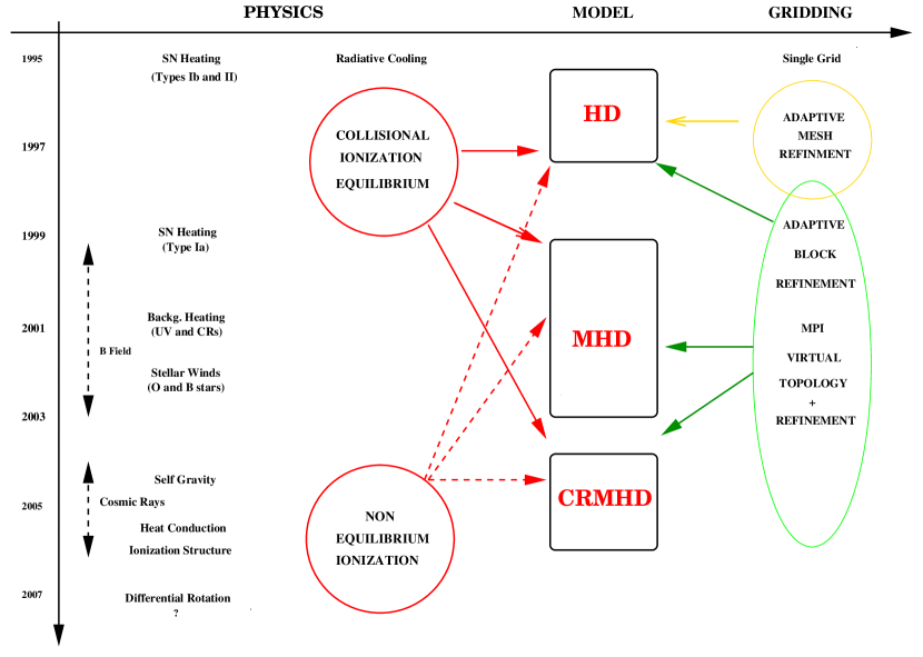
Figure 1: Structure and time schedule of the supernova-driven ISM model.

3 Characterizing Turbulence Scales in the ISM

The model can be used to characterize turbulence in the ISM and determine the integral scales at which the gas correlates both in time and space. The outer scale of the turbulent flow in the ISM is related to the scale at which the energy in blast waves is transferred to the interstellar gas. Such a scale can be determined by using the so-called two-point correlation function $R_{i,j}(\vec{r},t)=\langle u_{i}(\vec{x}+\vec{r},t)u_{j}(\vec{x},t)\rangle$, which in the case of isotropic turbulence can be written in terms of the scalar functions $f(r,t)$ and $g(r,t)$ as

$$R_{ij}(\vec{r},t)=\sigma^{2}(u)\left(g(r,t)\delta_{ij}+\left[f(r,t)-g(r,t)\right]\frac{r_{i}r_{j}}{r^{2}}\right),$$ (1)

where $\sigma^{2}(u)$ and $r_{i}$ are the variance of the velocity and the $i-$component of the displacement vector $\vec{r}$. If $\vec{r}$ is chosen to be oriented along the mean magnetic field ($x-$axis), $\vec{r}=r\vec{e}_{x}$, then

$$R_{11}/\sigma^{2}(u)=f(r,t),\quad R_{33}=R_{22}/\sigma^{2}(u)=g(r,t),~{}\mbox{and}~{}R_{ij}=0~{}\mbox{for}~{}i\neq j.$$ (2)

$R_{11}$ and $R_{22}=R_{33}$ are the longitudinal and transverse autocorrelation functions. The characteristic size of the larger eddies in the flow is given by the area under the curve of the autocorrelation function

$$L_{11}=\int_{0}^{+\infty}f(r,t)dr.$$ (3)

The left panel of Figure 2 shows the history of $L_{11}$ in the last 50 Myr of evolution of the magnetized ISM with mean field strengths of 2 (red) and 3 $\mu$G (black). The average integral length scales in both cases is 75 pc. There is a large scatter of $L_{11}$ around its mean as a result of oscillations in the momentary star formation rate, which is determined locally by density and temperature thresholds (note that in these simulations the mean SN rate is similar to the Galactic value), and on the formation of superbubbles, being responsible for the peaks observed in the two plots. The transverse integral length scale, $L_{22}$, given by

$$L_{22}=\int_{0}^{+\infty}g(r,t)dr=0.5L_{11}$$ (4)

in isotropic turbulence.

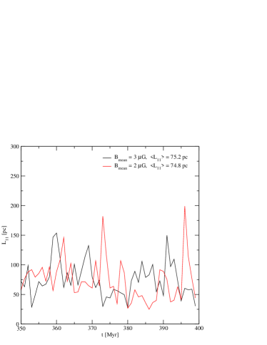
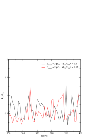
Figure 2: History of the characteristic size (given by $L_{11}$) of the larger eddies (left panel) and of the ratio $L_{22}/L_{11}$ (right panel) for the runs with mean field strengths of 2 (red) and 3 (black) $\mu$G.

However, in the present MHD simulations $0.2<L_{22}/L_{11}<1.3$ (right panel of Figure 2) for the two mean field strengths. In spite of the large scatter the time average of the $L_{22}/L_{11}$ over the 50 Myr period is 0.53 and 0.6 for $B_{mean}=2$ and $3~{}\mu$G, respectively, a value similar to the one predicted by (4). A similar behaviour is seen in the correlation functions calculated for the HD case, that is, there is a fluctuation of the ratio $L_{22}/L_{11}$ (Avillez & Breitschwerdt 2005c). In a statistical sense turbulence seems to be homogeneous and isotropic, but the history of the $L_{22}/L_{11}$ ratio indicates that this does not occur in general, and therefore, turbulence in the magnetized (and unmagnetized) ISM does not perfectly satisfy this.

It should be kept in mind that the relations (3) and (4) assume an isotropic and homogeneous (in the local sense) turbulent medium where energy is injected at the outer scales and transferred to the smallest scales, without any dissipation, until it reaches the Kolmogorov inner scale given by $R_{e}^{-3/4}l_{o}$ ($l_{o}$ is the injection scale), where it is dissipated by the molecular viscosity. Dissipation is a passive process as it proceeds at a rate determined by the inviscid inertial behaviour of the large eddies. Such an energy cascading corresponds to a divergence-free behaviour of the flow in the inertial range.

However, the ISM is a compressible medium swept up by shocks, which are in general more efficient in dissipating energy than molecular viscosity. Simulations of decaying sonic (Porter et al. 1998) and forced supersonic (Boldyrev et al. 2002) turbulence indicate that the ratio $\gamma=\langle u_{c}^{2}\rangle/\langle u_{s}^{2}\rangle$ that relates the compressional $u_{c}$ to the selenoidal $u_{s}$ component of the velocity field in the inertial range is smaller than 0.2. Thus, a small amount of energy is dissipated through shocks in the inertial range and the energy decay follows a quasi-Kolmogorov spectrum. The shock structures start to play an important rôle in energy transfer and dissipation near the dissipative range (Boldyrev 2002).

Jpeg image LB.jpg

Figure 3: Ovi contour map of a 3D Local Bubble simulation 14 Myr after the first explosion in the cluster. The LB is centred at (175, 400) pc and Loop I at (375, 400) pc.

4 Testing the Model

How much can the present SN driven ISM model setup be trusted? The answer to this question relies on the tests made with the numerical schemes and the physics approaches used in the ISM setup. The standard numerical tests carried out on the HD and MHD schemes showed that the code produces solutions, under different gas-dynamical conditions, that differ from the expected analytical and/or experimental solutions by at most $1\%$. Lately it has been claimed that a fundamental test of ISM models is the determination of the amount of Ovi column densities within a superbubble, similar to the Local Bubble (LB) (see Cox 2004; Breitschwerdt & Cox 2004). Observations along lines of sight near the disk within the Local Bubble and extending further away show that the Ovi column density (N(Ovi) ) has a mean value of $8\times 10^{12}$ cm^-2, with no values larger than $1.7\times 10^{13}$ cm^-2 according to FUSE observations (Oegerle et al. 2005). Therefore, in absorption, a fundamental test is the setup of the LB and the prediction of the Ovi and Hi column densities and the direct comparison with observed column densities.

Thus, we ran simulations following the evolution of the Local Bubble and Loop I as a result of clustered SN activity in an ISM disturbed by SN explosions at the Galactic rate. For this we took data cubes of previous runs with a finest adaptive mesh refinement resolution of 1.25 pc. We then picked up a site with enough mass to form the 81 stars, with masses, $M_{*}$, between 7 and 31 ${\rm M_{\odot}}$, that compose the Sco Cen cluster; 39 massive stars with $14\leq M_{*}\leq 31\,{\rm M_{\odot}}$ have already gone off, generating the Loop I cavity. Presently the Sco Cen cluster (here located at $(375,400)$ pc) has 42 stars to explode within the next 13 Myrs). We followed the trajectory of the moving subgroup B1 of Pleiades, whose SNe in the LB went off along a path crossing the solar neighbourhood (Figure 3). Periodic boundary conditions are applied along the four vertical boundary faces, while outflow boundary conditions are imposed at the top ($z=10$ kpc) and bottom ($z=-10$ kpc) boundaries. The simulation time of this run was 30 Myr, sufficiently long to cover the total evolution of both bubbles.

The locally enhanced SN rates produce coherent LB and Loop I structures (due to ongoing star formation) within a highly disturbed background medium. The successive explosions heat and pressurize the LB, which at first looks smooth, but develops internal temperature and density structure at later stages. After 14 Myr the LB cavity, bounded by an outer shell, which will start to fragment due to Rayleigh-Taylor instabilities in $\sim 3$ Myr from now, fills a volume roughly corresponding to the present day size (Fig. 3).

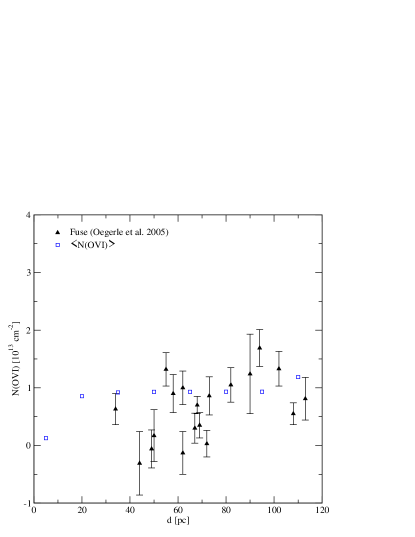
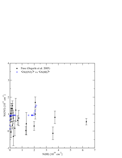
Figure 4: Variation of the calculated averaged Ovi column density with the distance (left panel) and with the calculated averaged Hi column density (right panel) within the Local Bubble for lines of sight with length $<120$ pc, and compared to FUSE observations.

The average Ovi and N(Hi) column densities, i.e., $\langle\mbox{{\rm N(O{\sc vi})\,}}\rangle$ and $\langle\mbox{{\rm N(H{\sc i})\,}}\rangle$, respectively, are calculated by averaging the column densities measured along 91 lines of sight (LOS) extending from the Sun and crossing Loop I from an angle of $-45^{\circ}$ to $+45^{\circ}$ (as shown in Figure 3) with angle increments of $1^{\circ}$. The left panel of Figure 4 shows $\langle\mbox{{\rm N(O{\sc vi})\,}}\rangle$ within the Local Bubble (i.e., for a LOS length $l_{LOS}<120$ pc) as function of distance (left panel) and of $\langle\mbox{{\rm N(H{\sc i})\,}}\rangle$ (right panel) at time 14.5 Myr of evolution after the first explosion and 0.5 Myr after the last explosion. Overlayed to both panels is the corresponding Ovi FUSE data taken from Oegerle et al. (2005). The clustered SN driven LB cavity simulated data shows that the averaged Ovi column density falls within the observed data and there is excellent agreement with respect to the observed distances. A similar result is found for the minimum and maximum column densities (see Breitschwerdt & Avillez 2005).

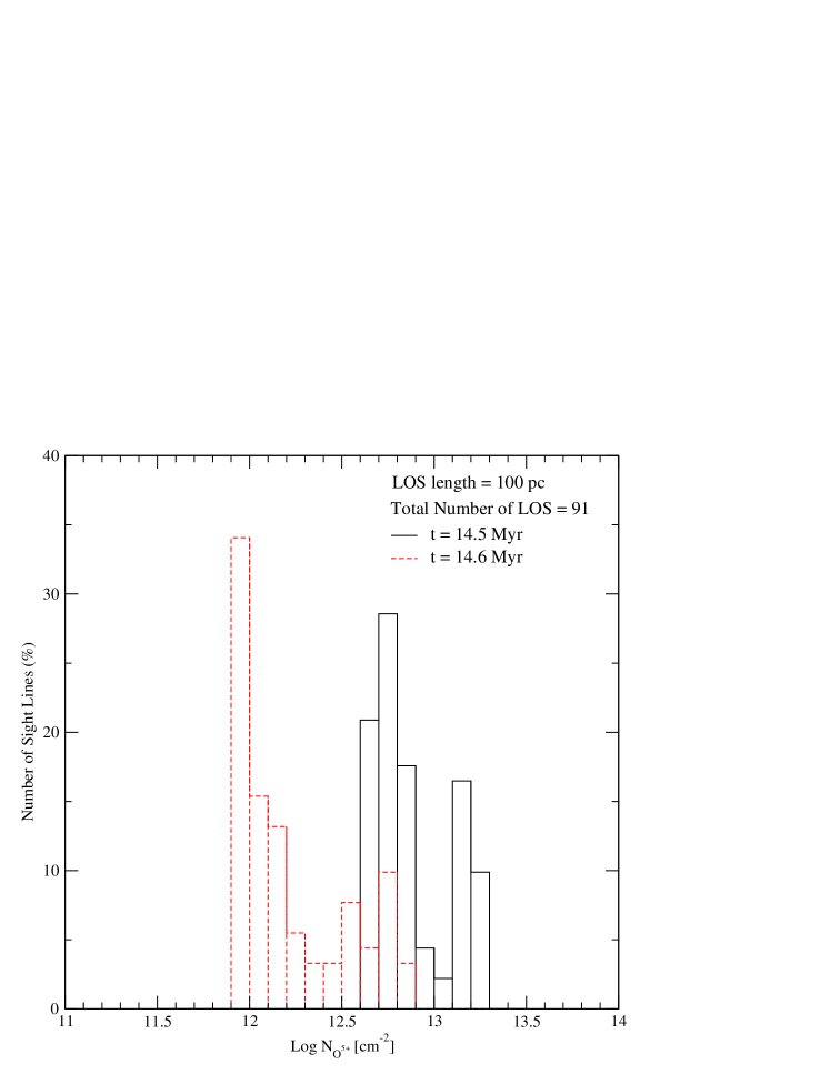
Figure 5: Histogram of the percentage of LOS with various ranges of observed N(O vi) within the LB at $t=14.5$ and $14.6$ Myr.

Histograms (Figure 5) of column densities obtained in the 91 LOS for $t=14.5$ show that 67% of the lines have column densities smaller than $10^{13}$ cm^-2 and in particular 49% of the lines have $\mbox{{\rm N(O{\sc vi})\,}}\leq 7.9\times 10^{12}$ cm^-2. There seems to be no correlation between the simulated N(Ovi) and N(Hi) , exactly like to what is observed (right panel of the figure), although the maximum averaged N(Hi) column density in the simulations is $2.1\times 10^{19}$ cm^-2, a value a little bit smaller than the observed one.

In the present model for $t\geq 14.5$ Myr the Ovi column densities are smaller than $1.7\times 10^{13}$ cm^-2 and $\langle\mbox{{\rm N(O{\sc vi})\,}}\rangle\leq 8.5\times 10^{12}$ cm^-2. These values are in excellent agreement with the mean column density of $7\times 10^{12}$ cm^-2 inferred from analysis of FUSE absorption line data in the Local ISM (Oegerle et al. 2005).

5 Final Remarks

The supernova-driven ISM model discussed here uses sophisticated numerical schemes and has proven to be a valuable tool in ISM studies. The results obtained with the ISM module in probing the evolution of the local ISM are in excellent agreement with those from recent observations by the FUSE satellite.

The present simulations still neglect an important component of the ISM, i.e., high energy particles, which are known to be in rough energy equipartition locally with the magnetic field, the thermal and the turbulent gas in the ISM. The presence of CRs and magnetic fields in galactic halos is well known and documented by many observations of synchrotron radiation generated by the electron component. The fraction of cosmic rays that dominates their total energy is of Galactic origin and can be generated in SN remnants via the diffusive shock acceleration mechanism to energies up to $10^{15}$ eV (for original papers see Krymsky et al. 1977, Axford et al. 1977, Bell 1978, Blandford & Ostriker 1978, for a review Drury 1983, for more recent calculations see Berezhko 1996). The propagation of these particles generates MHD waves due to the streaming instability (e.g. Kulsrud & Pearce 1969) and thereby enhances the turbulence in the ISM. In addition, self-excited MHD waves will lead to a dynamical coupling between the CRs and the outflowing fountain gas, which will enable part of it to leave the Galaxy as a wind (Breitschwerdt et al. 1991, 1993, Dorfi & Breitschwerdt 2005). Furthermore, as the CRs act as a weightless fluid, not subject to radiative cooling, they can bulge out magnetic field lines through buoyancy forces. Such an inflation of the field will inevitably lead to a Parker type instability, and once it becomes nonlinear, it will break up the field into a substantial component parallel to the flow (see Kamaya et al. 1996), thus facilitating gas outflow into the halo. We are currently performing ISM simulations including the CR and wave component.

References

- [2000] Avillez M. A., 2000, MNRAS, 315, 479
- [2001] Avillez M. A., & Berry, D. L. 2001, MNRAS, 328, 708
- [2004] Avillez M. A., & Breitschwerdt, D., 2004, A&A, 425, 899
- [2005] Avillez M. A., & Breitschwerdt, D., 2005a, A&A, in press [astro-ph/0502327]
- [2005] Avillez M. A., & Breitschwerdt, D., 2005b, in ”Astrophysics in the Far Ultraviolet - Five years of discovery with FUSE”, eds. G. Sonneborn, W. Moos, & B.-G. Andersson, ASP Conf. [astro-ph/0501466]
- [2005] Avillez M. A., & Breitschwerdt, D., 2005c, ApJ, in preparation
- [2001] Avillez M. A., & Mac Low, M.-M. 2001, ApJ, 551, L57
- [2002] Avillez M. A., & Mac Low, M.-M. 2002, ApJ, 581, 1047
- [1977] Axford, W.I., Leer, E., & Skadron, G. 1977, in Proc. 15th Int. Cosmic Ray Conf. (Plodiv) 11, 132
- [2001] Balsara, D. S. 2001, J. Comput. Phys., 174, 614
- [1978] Bell, A. R. 1978, MNRAS, 182, 147
- [1996] Berezhko, E. G. 1996, APh 5, 367
- [1989] Berger, M. J., & Colella, P. 1989, J. Comp Phys., 82, 64
- [2002] Berghöfer, T., & Breitschwerdt, D. 2002, A&A, 390, 299.
- [2002] Boldyrev, S. 2002, ApJ, 569, 841
- [2002] Boldyrev, S., Nordlund, Å, & Padoan, P. 2002, ApJ, 573, 678
- [2001] Breitschwerdt D. 2001, Ap&SS 276, 163
- [1991] Breitschwerdt, D., McKenzie, J.F., & Völk, H.J. 1991, A&A 245, 79
- [1993] Breitschwerdt, D., McKenzie, J.F., & Völk, H.J. 1993, A&A 269, 54
- [2004] Breitschwerdt, D., & Cox, D. P. 2004, in “How does the Galaxy Work?”, eds. E. Alfaro, E. Perez, & J. Franco, Kluwer (Dordrecht), p. 391
- [2005] Cox, D. P. 2004, Ap&SS, 289, 469
- [1998] Dai W., & Woodward, P. R. 1998, J. Comput. Phys., 142, 331
- [2005] Dorfi, E.A., Breitschwerdt, D. 2005, A&A, in preparation
- [1983] Drury, L. O’C. 1983, Rep. Prog. Phys. 46, 973
- [2003] Hanasz, M., & Lesch, H. 2003, A&A, 412, 331
- [1996] Kamaya, H., Mineshige, S., Shibata, K., & Matsumoto, R. 1996, ApJ, 458, L25
- [1977] Krymsky, G. F. 1977, Dokl. Nauk. SSR 234, 1306, (Engl. Trans. Sov. Phys. Dokl. 23, 327)
- [1969] Kulsrud, R. M., & Pearce, W. D. 1969, ApJ, 156, 445
- [1998] Mac Low, M.-M., Klessen, R. S., Burkert, A., & Smith, M. D. 1998, Phys. Rev. Lett., 80, 2754
- [2005] Oegerle, W. R., Jenkins, E. B., Shelton, R. L., Bowen, D. V., & Chayer, P. 2005, ApJ, 622, 3770
- [1998] Porter, D. H., Woodward, P. R., & Pouquet, A. 1998, Phys. Fluids, 10, 237
- [2003] Ryu, D., Kim, J., Hong, S. S., & Jones, T. W. 2003, ApJ, 589, 338
- [1998] Thornton, K., Gaudlitz, M., Janka, H.-Th. & Steinmetz, M. 1998, ApJ, 500, 95