On the nature of the X-ray source in GK Per

We report XMM-Newton observations of the intermediate polar (IP) GK Per on the rise to the 2002 outburst and compare them to Chandra observations during quiescence. The asymmetric spin light curve implies an asymmetric shape of a semi-transparent accretion curtain and we propose a model for its shape. A low Fe xvii ($\lambda\lambda$15.01/15.26 Å) line flux ratio confirms the need for an asymmetric geometry and significant effects of resonant line scattering.

Medium resolution PN spectra in outburst and ACIS-S spectra in quiescence can both be fitted with a leaky absorber model for the post shock hard X-ray emission, a black body (outburst) for the thermalized X-ray emission from the white dwarf and an optically thin spectrum. The difference in the leaky absorber emission between high and low spin as well as quasi-periodic oscillation (QPO) or flares states can be fully explained by a variation in the absorbing column density. For the explanation of the difference between outburst and quiescence a combination of the variation of the column density and the electron and ion densities is necessary. The Fe fluorescence at 6.4 keV with an equivalent width of 447 eV and a possible Compton scattering contribution in the red wing of the line is not significantly variable during spin cycle or on QPO periods, i.e. a significant portion of the line originates in the wide accretion curtains.

High-resolution RGS spectra reveal a number of emission lines from H-like and He-like elements. The lines are broader than the instrumental response with a roughly constant velocity dispersion for different lines, indicating identical origin. He-like emission lines are used to give values for the electron densities of $\log n_{e}\sim 12$. We do not detect any variation in the emission lines during the spin cycle, implying that the lines are not noticeably obscured or absorbed. We conclude that they originate in the accretion curtains and that accretion might take place from all azimuths.

1 Introduction

Cataclysmic variables (CVs) are interacting binaries consisting of a white dwarf that is accreting matter from a red dwarf star (often a main sequence star) due to Roche-lobe overflow (for an overview see Warner 1995). Intermediate polars are a subgroup of CVs, which typically have a non-synchronously spinning, magnetised white dwarf, and - if present at all - a truncated accretion disc. Thus, they fill the gap between the polars and non-magnetic dwarf novae. Accretion processes close to the white dwarf surface usually make them strong X-ray emitters.

GK Per turned into a nova in 1901 (Hale 1901, Pickering 1901) and is now observable as an intermediate polar (Watson et al. 1985). However, its nova shell is still visible at radio, optical, UV and X-ray wavelengths (Evans et al. 1992, Balman & Ögelman 1999, Anupama & Kantharia 2005). From a study of these shell ejecta Warner (1976) determined a distance to GK Per of 460 pc, confirming McLaughlin’s (1960) distance of 470 pc; only Duerbeck (1981) quotes an unpublished distance by McLaughlin of 525 pc. With an orbital period of about 2 days GK Per lies at the upper end in the period distribution of all known CVs. Thus, the geometrical dimensions are extremely large for a CV, noticeable mainly through the fact that the secondary has evolved to a K1 subgiant (e.g. Warner 1976, Morales Rueda et al. 2002).

GK Per shows dwarf nova type outbursts with a frequency of one in about 3 years, a typical duration of approximately 50 days (Šimon 2002) and an increase of 2.5 magnitudes in the optical. The slow rise to maximum light is probably caused by an inside-out outburst (Nogami et al. 2002) – in contrast to a more usual outside-in outburst – or a more complicated scenario, where the outburst starts at different distances from the disc centre (Šimon 2002).

Morales Rueda et al. (2002) investigated the absorption spectrum of GK Per’s companion star, deducing a mass ratio of $q=M_{K}/M_{wd}=0.55\pm 0.21$ and lower limits for the masses of the stars of $M_{K}\geq 0.48\pm 0.32$ M_⊙ and $M_{wd}\geq 0.87\pm 0.24$ M_⊙. The inclination angle is still uncertain, however, it must be smaller than 73^∘, since no eclipses are observed, and is probably larger than 50^∘ as can be deduced from models for GK Per’s accretion geometry (Hellier et al. 2004).

During the 1983 outburst Watson et al. (1985) discovered a clearly periodic signal attributed to the white dwarf spin. In quiescence, the spin light curve is double peaked (Patterson 1991, Ishida et al. 1992), while the outburst spin light curve typically shows a nearly sinusoidal behaviour (Hellier et al. 2004). Furthermore, during outburst the full amplitude of the variations is about 50% of the maximum value, while during quiescence it drops down to 20%.

In addition to the spin period, quasi-periodic oscillations (QPOs) have been discovered during outburst in the emission lines by Morales Rueda et al. (1996). Previously, Watson et al. (1985) reported a modulation of their EXOSAT (1.5-8.5 keV) data on a time scale of 2000 to $10\,000$ s. Subsequently, these QPOs have been observed also in the optical continuum (Morales Rueda et al. 1999, Nogami et al. 2002) and in the X-ray band by ASCA (0.7-10 keV, Ishida et al. 1996).

The QPO period varies between 4000 and 6000s, depending on the spectral range and on the time during the outburst. Hellier et al. (2004) suggest that the QPOs are caused by bulges travelling with an orbital period of about 5000s at the inner disc radius (instead of a bulge rotating with a period of 320 or 380s as suggested by Morales Rueda et al. 1999). Warner & Woudt (2002) already suggested such travelling waves that reach some height above the accretion disc allowing a temporary blockage of the view towards the white dwarf.

A few attempts have been made to fit the X-ray continuum spectrum ${\textstyle{\;\lower 3.01385pt\hbox{$>$}\;\atop\raise-0.3014pt\hbox{$\sim$}}}1$ keV of GK Per (EXOSAT, Watson et al. 1985; Norton et al. 1988; GINGA, Ishida et al. 1992) using power-law and bremsstrahlung components. The most convincing model appears to be that applied by Ishida et al. (1992) who fitted a leaky absorber model to the spectral emission in the range 2-30 keV. Even in early X-ray spectra and all subsequent observations a prominent Fe fluorescence at 6.4 keV has been detected (e.g. Watson et al 1985; Ishida et al. 1992; Hellier & Mukai 2004). Hellier & Mukai claim that the red wing of the line in their Chandra data is due to the movement of the in-falling material.

Wu et al. (1989) and Yi & Kenyon (1997) find a very flat UV spectrum ($\log$ Flux (erg cm^-2 s^-1 Å^-1) $\approx$ -11.75 over the range 1000 to 3500 Å) which they explain with a truncated accretion disc. Since a magnetic model is not successful, they suggest X-ray heating. However, as the increase in X-ray emission during outburst is insufficient, they suggest that most of the accretion energy is radiated at extreme UV wavelengths. Yi et al. (1992) further find that the observed X-ray flux varies only moderately in spite of large variations in the mass accretion rate $\dot{\cal M}$ during an outburst. They explain this observation by obscuration of the hard X-rays during outburst due to an increased disc thickness.

In this paper we re-examine the X-ray characteristics by analysing the XMM-Newton EPIC light curves and continuum spectra and investigate high-resolution RGS line spectra. Mauche (2004) mentioned these data briefly and confirm the strong Fe K-shell emission at 6.4 keV. Furthermore, they detect H- and He- like emission lines of N, O, Ne, Mg, Si and S and possibly He-like Al. Furthermore, we compare these outburst data to X-ray data during quiescence obtained with Chandra ACIS-S. Balman (2001) has analysed in particular the shell emission and found it to be a multi-temperature adiabatic shock region with enhanced abundances of Ne and N.

2 The observations

Table 1: Observations log. All observations were taken on 9 March 2002. Gaps are not listed, but are obvious from Fig. 2.

Instrument	Data Mode	Filter	Start UT	Stop UT
M1	Imaging	Medium C	14:49:13	23:38:53
M2	Imaging	Medium C	14:49:08	23:38:53
OM	Imaging & Fast	U	14:46:44	18:01:00
OM	Imaging & Fast	B	18:06:36	20:50:52
OM	Imaging & Fast	UVW1	20:56:30	23:06:46
PN	Imaging	Medium	15:22:30	23:34:10
R1	Spectroscopy		14:42:54	23:42:26
R2	Spectroscopy		14:42:54	23:42:26

GK Per was observed with XMM-Newton on 9 March 2002 during the early phase of the 2002 outburst, approximately 1.5 optical magnitudes below and 30 days before the maximum light. According to the AAVSO light curves the whole outburst lasted about 70 days. The data consist of 32 ks (9 $h$, i.e. only about 20% of a GK Per’s orbit) observing time using all instruments on board XMM-Newton (EPIC PN and MOS1+2, RGS1+2, OM). The OM data were taken consecutively in the filters U (7.5 ks), B (9.9 ks), UVW1 (7.8 ks). For the reduction we used the standard SAS software (version 6.0.0). Only for the OM data we used the pipeline products.

We checked the data for pile-up and found evidence for pile up for energies above $\sim 7$ keV. Thus, during extraction of the spectra we dismissed central pixels of the stellar image on the CCD chip until no sign of pile-up was present. Furthermore, at the beginning of the observing run and between 2 and 5 hours after the start of data taking the background on the PN CCD chip is unusually high, possibly due to a minor solar flare. To avoid a contamination of the object spectrum we only used times with a low background for the extraction of the spectra.

For the extraction of the light curves, the pile-up and high background is not a problem, as the flux is conserved and the light curves are background subtracted. However, the PN detector suffered failures on short timescales during the exposure run (at the times of the high background), leading to drops in the light curve as noticeable in Fig. 2 between 0 and 0.5$h$ and between 2 and 5$h$. We still used the full data set for the light curve extraction. Due to technical problems with the B filter (it has the highest count rate which lead to artifacts that could not satisfactorily be corrected) we did not use the B data for our analysis. No such problems affected the U and UVW1 data.

A high-resolution image of GK Per was taken with the ACIS-S detector aboard Chandra on 10 Feb 2000 for 96.55 ks. Apart from the point source the expanding shell can clearly be recognised in X-rays. We colour-coded the photon energies and produced a smoothed image (displayed in Fig. 1), demonstrating that the expanding shell is a much softer X-ray source than the central star. Contrary to Balman (2001) we calculated individual spectra for the nova and the shell by selecting the central source and those parts of the shell which are brightest in this image (banana shaped region in the south western quadrant outside a radius of 20 arcsec to avoid contamination/pile-up of the shell by the source), respectively.

In order to avoid pile-up of the quiescent source spectrum we chose an annular extraction region with an inner radius of 3 pixels ($\approx 1.5$″), thus excluding the innermost photons from the analysis which are suffering from pile-up. The effective areas calculated by the CIAO software account for the fact that the innermost region is excluded implying the known behaviour of the point spread function and spectral analyses can still be carried out with lower signal-to-noise. For a more detailed study of the pile-up problem in this particular data set see Balman (2005).

In order to check whether the emission in the shell was caused by a reflection effect from a previous outburst, we checked the long term light curve in the AAVSO Data base. However, the previous outburst took place nearly one year (March/April 1999) before the Chandra quiescent data were obtained (Feb 2000). With a maximal size of 50” and a distance of 460 pc the light travel time from the nova to the brighter parts of the shell would be maximally about 130 days which excludes any re-brightening effects.

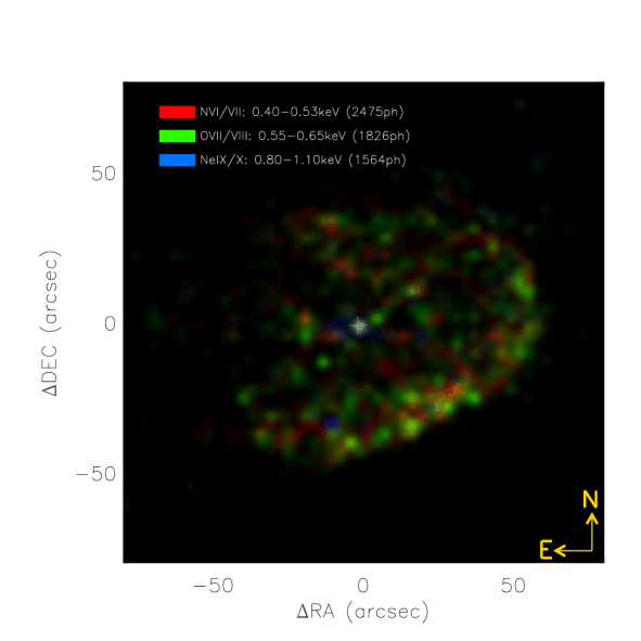
Figure 1: Smoothed ACIS-S image of GK Per. The colours represent different photon energies ranges as indicated in the plot.

3 Light curves

Figure 2: EPIC (PN, MOS1 and MOS2) and Optical Monitor (U, UVW1) light curves as indicated. All except the PN light curves are shifted upwards for clarity of the plot, the dashed lines indicate the zero level for the light curve immediately above (identical zero line for U and UVW1 light curve).

In Fig. 2 we show the XMM-Newton X-ray and UV light curves of GK Per; $t=0$ corresponds to the start time of the PN observation. The OM monitor observations consist of 4 stretches of data in each of the filters U, (B left out) and UVW1. The gaps are actual gaps in the data acquisition.

The PN light curve shows two prominent peaks - or flares - occurring at 1.5$h$ and 7$h$, which can also be identified in the MOS light curves. Note that the background at these times is particularly low, thus the flares must originate in the source. These X-ray flares appear to coincide with minima in the UV light curves and might be linked to the QPO cycle (see below). To check the spectral behaviour of the X-ray emission we split up the light curves into a hard and a soft X-ray component (soft: $<1$ keV, hard: $>1$ keV; Fig. 3). Clearly, the flares are dominant in the soft component, i.e. the flares must originate mainly from the thermalized emission on the white dwarf surface.

Figure 3: Light curve of the soft ($<1$ keV, black body, shifted upwards by 30 counts/s for clarity) and hard ($>1$ keV, bremsstrahlung) components. Notice that the flares are dominant in the soft component.

Figure 4: Power spectrum of the EPIC data. Clearly visible are the fundamental and the first harmonic of the spin period at 351.3s and 175.5s. The power spectra for the MOS light curve are shifted upwards by 50 units each for clarity of the plot.

Consider next the power spectrum of the PN light curve (shown in Fig. 4). The white dwarf spin period of 351 s is clearly visible, the wide width of the power spectrum peak is due to the short observing run and excludes further analyses of the evolution of the spin up (Mauche 2004). It is interesting, that the OM data do not show any significant peak at the spin period of the white dwarf.

Figure 5: EPIC light curve folded on the spin period of the white dwarf, 351.26 s. For clarity, two spin cycles are plotted.

Figure 6: EPIC and OM light curves folded on the 5000 s (QPO) period. Note that only the UVW1 light curve is shifted upwards by 10 counts/s, all other light curves are at their original values. Note also that the UV light curves only cover about one QPO cycle each. For clarity, two cycles are plotted.

Fig. 5 shows the EPIC light curves folded on the spin period. The full amplitude in the PN light curve is about 39% of the maximum value, slightly less than observed by Hellier et al. (2004) who report a variation of 50% at a comparable time during rise into outburst. During quiescence, the same variations lie between 15% and 20% (Norton et al. 1988). Our observed spin profile clearly appears asymmetric: the rise to the spin light curve maximum is significantly longer than the sudden drop from maximum to minimum. This shape is obvious in all three EPIC light curves. While Hellier et al. still find a nearly sinusoidal shape, their spin light curves show a similar tendency. Also the quiescent X-ray spin light curve shows the slow rise and sudden drop (Norton et al. 1988).

Figure 7: Light curves of the soft ($<1$ keV) and hard ($>1$ keV) component folded on the Spin period of the white dwarf, 351.26 s. For clarity, two spin cycles are plotted.

In order to check for any difference between the soft and hard components (see next Section), we calculated the light curve for the soft and hard spectral range. As Fig. 7 implies, the relative difference between the two components in terms of the variation of the spin period is nearly identical and thus identical to the amplitude of the total variation of 39%.

Figure 8: Light curves of the soft ($<1$ keV) and hard ($>1$ keV) component folded on the 5000 s (QPO) period. For clarity, two cycles are plotted.

Our XMM-Newton data are compatible with the 5000 s QPOs found before (e.g. Morales Rueda et al. 1999, Fig.4), with again a broad peak in the power spectrum due to the short observing run. It is interesting to note that the UV light curves seem to show an anti-correlated behaviour regarding the QPOs. However, the UV data sets each cover only one QPO cycle and therefore cannot serve for a rigorous period analysis. It might be that the anti-correlated behaviour only appears at the same time as flares appear.

Fig. 8 shows the soft and hard X-ray light curves folded on the 5000 s (QPO) period. The variation on this period is clearly much stronger in the soft component, where we measure an amplitude of 58% of the maximum, than in the hard component, where the amplitude is only about half (30%) as large.

Figure 9: PN light curve. Over-plotted is the light curve phased on the 5000 s (QPO) period. It is obvious that the flares coincide with the maxima in the 5000 s cycle and thus dominate the variation.

Reexamining the flares shows a correlation with a maximum in the 5000 s (QPO) variation (Fig. 9), and thus dominate the signal. Removing the flares from the light curves reduces the 5000 s (QPO) signal in the power spectrum significantly by a factor of 4 (comparable in strength to the minor peak at 2000 s) and shifts it to approximately 5500 s. However, the power spectrum for periods $<1000$ s is unchanged.

4 Medium resolution spectroscopy

Fig. 10 shows the EPIC-PN spectrum of GK Per together with a fit to the data. Following the approach by Ishida et al. (1992) we chose a leaky absorber model for the hard X-ray spectrum, and added a blackbody spectrum for the soft X-ray emission representing the thermalized emission from the white dwarf and a mekal spectrum for the optically thin emission. The leaky absorber consists of two bremsstrahlung components with identical temperatures but different column densities to allow for structured absorption, thus representing a simple model of a possibly much more complex situation with a range of column densities due to inhomogeneous in-falling material. However, this two-component approach represents a simple blobby accretion model. On top of these continuum spectra we added a simple Gaussian to account for the Fe fluorescence line at 6.4 keV. The resulting fit has a reduced $\chi^{2}$ of 0.91.

Our model fits the data well, but not perfectly. The fit residuals (also shown in Fig. 10) are most prominent in the region 0.5 to 0.6 keV. This happens to be the spectral region covered by the RGS instruments and, as shown in Section 5, we see line emission (in particular H-like N vii at $\sim$ 0.9 keV) that is not appropriately described by the models used. Also, the single temperature black body is only a simple approximation of a possibly far more complex temperature structure.

The flux over the total observed range in PN (0.17 to 15 keV, corrected for the missing central pixel) is $F_{total}=2.82\times 10^{-10}$ erg cm^-2 s^-1; for comparison with Hellier et al. (2004) we also compute the flux in the energy range 2 to 15 keV as $F_{2-15keV}$ = $2.73\times 10^{-10}$ erg cm^-2 s^-1, i.e., the soft component contributes very little to the total X-ray flux. Due to the pile-up correction an error of approximately 10% is introduced in the flux estimates (Robrade 2005, private communication). Hellier et al. observed a mean flux during rise and maximum of the 1996 outburst of $F_{2-15keV;H}=5.0\pm 0.8\times 10^{-10}$ erg cm^-2 s^-1, similar to Ishida et al.’s (1992) value for the 1989 outburst of $F_{2-20keV;I}=4.8\pm 1.7\times 10^{-10}$ erg cm^-2 s^-1. Using a distance of 460pc our flux value leads to a luminosity of $L_{2-15keV}=6.91\times 10^{33}$ erg s^-1 ($L_{total}=7.14\times 10^{33}$ erg s^-1).

Our column densities of the leaky absorber of $(2.20\pm 0.14)\times 10^{23}$ cm^-2 and $(3.67\pm 0.23)\times 10^{22}$ cm^-2 are almost an order of magnitude smaller than those determined by Ishida et al. (1992) who caught GK Per on early decline from outburst (approximately 0.5 mag below maximum light).

The leaky absorber model is certainly not the only possible model that one could fit to the data. Instead of the leaky absorber model we also tried a warm absorber (single bremsstrahlung component) without success (unacceptable fit with a $\chi^{2}=12$), a single black body ($\chi^{2}=5.4$) and a single black body plus an optically thin component (raymond). The latter fit is better but not acceptable ($\chi^{2}=1.75$). Furthermore, physically we expect bremsstrahlung to originate in the post shock portion of the accretion column as the material cools while it settles onto the white dwarf (see e.g. King 1995).

The addition of the mekal model improved the fit slightly with a $\chi^{2}$ of 0.906 in comparison to the simpler model with a $\chi^{2}$ of 0.973. An exchange of the mekal model with a raymond model yields no difference ($\chi^{2}=0.914$) and the parameter values are identical within the error ranges. In particular, the parameters of the raymond model lie within the error range of the mekal parameters (raymond: $n_{H}=1.317\pm 0.072$; $kT=0.807\pm 0.029$; $norm=0.0107\pm 0.0015$).

On the other hand, a more complicated model allowing for a range of temperatures in the black body component does not seem necessary regarding the good fits to the data. However, a realistic accretion column will certainly show a range of temperatures between the shock and the white dwarf’s surface.

Figure 10: The PN continuum spectrum with a leaky absorber (hard X-rays), a blackbody component (soft X-rays), a mekal component and a Gaussian (Fe fluorescence at 6.4 keV) spectral fit ($\chi^{2}=0.91$).

Table 2: Fit parameters of the continuum fit (model: wabs(blackbody) + wabs(bremsstrahlung) + wabs(bremsstrahlung) + wabs(mekal) + gauss), $\chi^{2}=0.906$.

Parameter	Type of model	Unit	value	error
$n_{H}$		$10^{22}$cm-2	21.98	1.37
kT	bremsstrahlung	keV	10.56	0.81
norm1	bremsstrahlung		0.0801	0.0052
$n_{H}$		$10^{22}$cm-2	3.67	0.23
kT	bremsstrahlung	keV	10.56∗	0.81∗
norm1	bremsstrahlung		0.0240	0.0018
$n_{H}$		$10^{22}$cm-2	0.315	0.019
kT	black body	keV	0.05961	0.00027
norm2	black body		0.0119	0.0048
$n_{H}$		$10^{22}$cm-2	1.306	0.068
kT	mekal	keV	0.761	0.038
norm3	mekal		0.0112	0.0017
$E$	Gaussian	keV	6.475	0.015
$\sigma$	Gaussian	keV	0.274	0.020
norm4	Gaussian		0.00121	0.00014

^∗ value set equal to value of other bremsstrahlung component.

¹ norm(brems) = $3.02\times 10^{-15}/(4\pi D^{2})\int n_{e}n_{I}dV$, where $D$ is the distance to the source (in cm) and $n_{e}$, $n_{I}$ are the electron and ion densities (in cm^-3).

² norm(bbody) = $L_{39}/D_{10}^{2}$, where $L_{39}$ is the source luminosity in units of $10^{39}$ erg s^-1 and $D_{10}$ is the distance to the source in units of 10 kpc. With a distance of 460 pc this yields a luminosity for the black body component $L=1.7\times 10^{33}$ erg s^-1.

³ norm(mekal) = $(10^{-14}/(4\pi(D_{A}(1+z))^{2}))\int n_{e}n_{H}dV$ , where $D_{A}$ is the angular size distance to the source (cm), $n_{e}$ and $n_{H}$ are the electron and H densities (cm^-3)

⁴ norm(gaussian) = total photons cm^-2 s^-1 in the line.

Figure 11: Fe fluorescence line with the model fit (upper panel) and the residuals (bottom panel).

The line flux in the Fe fluorescence line is measured as $1.25\times 10^{-11}$ erg cm^-2 s^-1 ($1.21\times 10^{-3}$ photons cm^-2 s^-1), a factor two less than determined by Ishida et al. (1992) during the 1989 moderate outburst. The line has an equivalent width of 447 eV, considerably more than in Hellier & Mukai’s (2004) observations who measure an equivalent width of 260 eV. Closer inspection of Fig. 11 suggests that our value might be overestimated as the single Gaussian fit to the Fe fluorescent line is not satisfactory: the center of the line seems narrower than the fitted Gaussian and there seems to exist a broad underlying component, especially redwards of the line. This emission in the red wing of the fluorescence line might be Compton scattering due to K-shell fluorescence in the white dwarf atmosphere as discussed by van Teeseling et al. (1996). In this case, fluorescence in the accretion column would be less significant. However, Hellier & Mukai (2004) attribute this emission to infalling pre-shock material with velocities up to 3700 km s^-1.

Interestingly, the variation of the Fe fluorescence line on the spin cycle is relatively weak. While the total PN light curve shows a variation of 39%, the Fe fluorescence line light curve (including continuum) shows a variation of only 28% (Fig. 5). Considering the strong continuum at this wavelength (about 2/3 of the total flux at this wavelength) this amounts to a negligible variation of the fluorescence line. On the 5000 s (QPO) period the variation is also negligible.

In order to verify a change in the amount of absorbing material as a function of spin cycle we extracted PN-data for high and low spin phases and fitted both spectra with the leaky absorber plus black body model, keeping all parameters fixed except the column densities. The resulting fits with $\chi^{2}$ values of 0.86 and 0.81 are better than the original fit to the spin cycle averaged data ($\chi^{2}=0.91$). The column densities change significantly and are much better defined in the separate fits – as implied by the smaller errors (see Table 3).

Table 3: Fitted column densities (in units $10^{22}$cm^-2) and equivalent width (EW) of the fluorescence line (in eV) for the averaged spectrum (see Table 2) as well as for the spin and 5000 s (QPO) cycle high and low states. The given flux is in units of $10^{10}$ erg cm^-2 s^-1.

model	average	$\sigma$	high state	$\sigma$	low state	$\sigma$	QPO high state	$\sigma$	QPO low state	$\sigma$
brems	21.98	1.37	17.54	0.29	32.54	0.61	19.69	0.33	26.31	0.48
brems	3.67	0.23	3.049	0.055	5.180	0.104	2.720	0.047	5.93	0.13
bbody	0.315	0.019	0.2954	0.0013	0.3435	0.0018	0.2809	0.0012	0.3746	0.0021
mekal	1.306	0.068	1.295	0.026	1.432	0.029	1.231	0.023	1.581	0.037
$\chi^{2}$	0.91		0.86		0.81		0.80		0.80
Flux	2.82		3.03		2.45		2.98		2.57
EW	447		417		523		430		483

Similarly, we extracted the spectra during high (flare) and low phase of the 5000 s (QPO) variation. These changes between (QPO) high and low state can also solely be explained by a variation in the column density. The column densities are listed in Table 3. It is interesting to note that the variation in the column density during the spin cycle is strongest in the bremsstrahlung component and during the 5000 s (QPO) cycle (the flares) strongest in the black body component.

5 High-resolution spectroscopy

Figure 12: O viii, N vii (H-like) and O vii, N vi (He-like) emission lines in RGS1 (left) and RGS2 (right). The FWHM values are denoted by $\sigma$ in the figures.

Figure 13: Fe xvii emission line. Note, that the 15.26  Å intersystem line is stronger than the 15.01  Å resonance line.

5.1 H-like and He-like emission lines

The XMM-Newton reflection grating spectrometers cover the energy range between 0.3 - 2 keV, where the overall X-ray flux in the medium resolution spectrum is lowest. Despite the overall rather low signal-to-noise ratio of the RGS data, a multitude of emission lines can be detected. The line features can be identified as O viii, N vii (both H-like) as well as O vii and N vi (both He-like); in order to give an impression of the RGS data we plot the most prominent emission lines in the RGS1 and RGS2 spectra in Fig.12.

In Table 4 we list the line counts, line widths and identifications of other He-like and H-like lines found in the spectra. The line fluxes were obtained with the CORA program (Ness & Wichmann 2002). The line profiles were approximated by analytical profile functions, where the Full Width at Half Maximum (FWHM) can be iterated. We found that all lines are significantly broader than the instrumental broadening profiles (FWHM$=0.06$ Å), so physical line broadening mechanisms are required. The instrumental broadening can roughly be described by a Lorentzian profile. However, for the broadened lines of O viii, O vii and N vi we found Gaussian profiles to fit the RGS data much better than Lorentzians. The FWHM values increase with increasing wavelength indicating similar velocities for these lines ($\sim 1600-1800$ km s^-1). The N vii line at 24.8 Å shows a totally different profile with three obvious components (upper right in Fig.12. We approximated these by Lorentzian profiles (since they are more affected by the instrumental line broadening).

5.2 Fe xvii emission lines

Let us focus next on the Fe xvii lines at 15.01 Å and 15.26 Å, shown in Fig.13. These lines are fitted best with Lorentzian profiles. The line at 15.26 Å is clearly stronger than the 15.01-Å line, an interesting finding since the 15.01-Å line is the strongest resonance line of the Fe xvii species (2p^6 1S₀–2p⁵ 3d ¹P₁) involving high transition probabilities, while the 15.26-Å line is an intersystem line (2p${}^{6}\,{}^{1}$S₀–2p⁵3d ³D₁) with correspondingly lower transition probabilities. Of course, the identification might be incorrect and we are actually dealing with the O viii Ly_γ-line expected at 15.17Å. However, the interpretation as O viii Ly_γ implies a red shift, which we do not see in the other lines of the O viii Ly series nor in any other line. We therefore conclude that the line measured with 44 counts must be attributed to the 15.26-Å line of Fe xvii, while the 15.01-Å line is only measured with at most 25 counts. The errors are quite large, but the ratio of $\lambda 15.01/\lambda 15.26$ is, within the errors, less than unity.

Since both lines originate from the same ionization stage of the same element, this cannot be attributed to temperature or abundance effects. At any temperature capable of producing the ionization stage of Fe xvii the ratio is expected to be of order 3-4. The only scenario explaining the measured line ratio is resonant scattering, i.e., reabsorption of photons emitted from transitions with high radiative absorption probabilities and reemission into any other direction. In symmetrical emission regions the effect balances out by some photons being scattered out of the line of sight and others being scattered into the line of sight. However, in asymmetric geometries like accretion discs and curtains, resonant line scattering can lead to an effective loss of resonance line photons. Lines with low oscillator strengths (like the 15.26-Å line) are much less affected by resonance scattering.

We tested this scenario by searching for other lines of Fe xvii with low oscillator strength, and found another line at 16.78 Å (2p${}^{6}\,{}^{1}$S₀–2p⁵3s³P₁) to be suspiciously strong compared to the 15.01-Å line. This supports the above explanation and we therefore conclude that the regions emitting Fe xvii come from asymmetric plasma with high densities or long path lengths. We further note that the oxygen emission cannot originate from the same regions, because the same effect would have to be observed in an absence of the Ly_α-line and a stronger presence of the Ly_β-line, which is not the case. One could argue that the Ly_α and the Ly_β-lines are affected by resonant scattering while the Ly_γ-line is not (and it would be the true interpretation of the 15.26 Å feature). However, this also requires resonant scattering to be at work (only for oxygen instead of iron), but would still not explain the red shift and the relative strength of the 16.78-Å line. We thus consider it most likely that iron is emitted in a different geometry (where resonance photons are lost) than oxygen (regions which are either optically thin or are more symmetric).

5.3 Densities

He-like triplets can be used for plasma density diagnostics using the density-sensitive f/i line flux ratios. This technique was originally developed by Gabriel & Jordan (1969) for solar X-ray data and has recently been applied by, e.g., Ness et al. (2004) to analyze a large number of stellar coronal emission line spectra. In the bottom left of Fig. 12 we show the O vii triplet with the triplet lines marked by r (resonance line), i (intercombination line) and f (forbidden line). The forbidden line is quite faint, while the intercombination line has almost the same flux as the resonance line (within the errors). In plasma with an electron density below $10^{11}$ cm^-3 the line flux ratio f/i is greater than one. From the measured ratio f/i$\sim 0.3$ we formally derive a density of $\log n_{e}\sim 11.6\,\pm\,0.1$ cm^-3. This number assumes negligible radiative deexcitations of the forbidden line level. However, in the presence of UV radiation fields, the transition from f to i can also be triggered by photons and thus mimic high densities. We have performed a crude estimate of these effects using the UV flux measurements by Wu et al. (1989) and Yi & Kenyon (1997), who find a very flat UV spectrum with $\log$ Flux (erg cm^-2 s^-1 Å^-1) $\approx$ -11.75 over the range 1000 to 3500 Å . As in Ness et al. (2001) we convert this flux to a black-body temperature, which can be used to predict a correction term in the density determination. We find a corresponding black-body temperature of $<2000$ K assuming a wavelength for the transition f to i of 1636 Å. With such a low temperature any effects from the UV radiation field can be neglected for all He-like ions. We additionally use the N vi and Ne ix He-like triplets and find $\log n_{e}=11.57\pm 0.1$ for N vi and $\log n_{e}=12.1\,\pm\,0.3$ for Ne ix.

The densities and the line flux ratio $\lambda 15.01/\lambda 15.26$ can be explored with a few assumptions to estimate the path length $\ell$. First we assume a simple ”escape factor” model (escape factor $P(\tau)\approx[1+0.43\tau]^{-1}$ for a homogeneous mixture of emitters and absorber in a slab geometry; e.g., Kaastra & Mewe 1995, Mewe et al. 2001). The escape factor can be calculated from the measured line flux ratio and the line flux ratio in an optically thin plasma (i.e., the unabsorbed line flux ratio). The unabsorbed ratio is somewhat uncertain with values up to four (from theoretical calculations; e.g., Brown et al. 1998, Bhatia & Doschek 1993) and values in the range 2.8-3.2 (from laboratory measurements in the Livermore Electron Beam Ion Trap EBIT). Systematic measurements of the $\lambda 15.01/\lambda 15.26$ ratios have been carried for a large sample of stellar coronae by Ness et al. (2003) yielding an average value of $\sim 3$, which we use here. The formal measured ratio is $\lambda 15.01/\lambda 15.26\approx 0.6$ and the escape factor $P(\tau)\approx 0.2$. The escape factor model allows us to calculate an optical depth $\tau\approx 10$.

The equation

$$\tau=1.2\ 10^{-14}\left(\frac{n_{i}}{n_{el}}\right)A_{z}\left(\frac{n_{H}}{n_{e}}\right)\lambda\ f\sqrt{\frac{M}{T}}{n_{e}}\ell$$ (1)

(e.g., Mewe et al. 2001) describes the optical depth $\tau$ as a function of some ion-specific parameters and the product of electron density $n_{e}$ (cm^-3) and path length $\ell$ (cm). Further, $n_{i}/n_{el}$ is the fractional ionisation, $A_{z}=n_{\rm el}/n_{\rm H}$ is the elemental abundance, $n_{H}/n_{e}=0.85$ is the ratio of hydrogen to electron density, $f$ is the oscillator strength, $M$ is the atomic number, $\lambda$ is the wavelength of the resonance line (Å) and $T$ is the temperature (K). From the optical depth $\tau\approx 10$, derived from $\lambda 15.01/\lambda 15.26$ line ratio, a characteristic plasma dimension $\ell$ can be estimated for the $\lambda=15.01$-Å line. Using $M=26$ (for iron), $f=2.6$ (for the ¹S₀–¹P₁ transition at 15.01 Å), $T=7\times 10^{6}$ K. We further assume an ionisation fraction $n_{i}/n_{el}=0.25$ in Fe xvii (Arnaud & Raymond 1992) and cosmic Fe abundance. With these parameters we compute from Eq. 1 and the measured value $\tau\approx 10$ the product $n_{e}\ell=1.3\times 10^{21}$ cm^-2. The electron density $n_{e}$ can only be roughly estimated from the He-like triplet diagnostics, which consistently yields values $\log n_{e}\sim 11.8$. Note, however, that the iron lines might originate from totally different regions than the He-like lines and these density estimates might not be valid. With this value we find a formal path length of $\ell=2\times 10^{9}$ cm with considerable uncertainty.

5.4 Variation of emission lines?

An extraction of line profiles of O viii, N vii and N vi for high and low, pole approaching or pole receding spin phases shows no significant variation (no detectable line strength variation or line shifts) with spin cycle. These emission lines also show no significant variation on the 5000 s (QPO) cycle (or rather with the flares) with the given quality of the RGS spectra.

Table 4: Lines identified in RGS spectra.

$$\begin{array}[]{llcrclrcl}\vskip 3.0pt plus 1.0pt minus 1.0pt\cr\hline\cr\vskip 3.0pt plus 1.0pt minus 1.0pt\cr Line}{&{\hskip 8.61108pt}\lambda_{0}\leavevmode\nobreak\ (\AA)}{&RGS&{\hskip 8.61108pt}Counts&&FWHM&{\hskip 8.61108pt}\lambda\leavevmode\nobreak\ (\AA)&{\hskip 4.30554pt}T_{max}\\ \vskip 3.0pt plus 1.0pt minus 1.0pt\cr\hline\cr\vskip 3.0pt plus 1.0pt minus 1.0pt\cr\lx@intercol\rm\bf H-like\ ions\hfil\lx@intercol&&(\AA)&\\ \hline\cr{\mathrm{SiXIV}}&6.180&2&48\,\pm\,11&&0.047^{a}&6.1800&7.11\\ \hline\cr{\mathrm{NeX}}&12.132&2&73\,\pm\,12&&0.08^{a}&12.16&6.76\\ \hline\cr{\mathrm{OVIII}}&16.003&1&25\,\pm\,\ 7&&0.05^{a}&16.003&6.50\\ {\mathrm{OVIII}}&&2&30\,\pm\,\ 8&&0.05^{a}&16.003&\\ \hline\cr{\mathrm{OVIII}}&18.971/&1&127\,\pm\,13&&0.12^{b}&19.003&6.48/9\\ &\ \ 18.977&2&186\,\pm\,17&&0.12^{b}&19.0019&&\\ \hline\cr{\mathrm{NVII}}&24.779/&2&85\,\pm\,16&&0.06^{a}&24.7431&6.32\\ {\mathrm{NVII}}&\ \ 24.785&2&211\,\pm\,21&&0.06^{a}&24.8294&\\ {\mathrm{NVII}}&&2&128\,\pm\,20&&0.06^{a}&24.9544&\\ \hline\cr{\mathrm{NVII}}&total&2&424\,\pm\,31&&&24.8423&\\ \hline\cr\hline\cr\lx@intercol\rm\bf He-like\ ions\hfil\lx@intercol\\ \hline\cr{\mathrm{SiXIII}}&6.648&2&43\,\pm\,13&&0.047^{a}&6.6500&7.01\\ {\mathrm{SiXIII}}&6.688&2&2\,\pm\,\ 2&&0.047^{a}&6.6900&6.99\\ {\mathrm{SiXIII}}&6.740&2&21\,\pm\,10&&0.047^{a}&6.7400&7.00\\ \hline\cr{\mathrm{SiXIII}}&total&2&66\,\pm\,19&&&&7.03\\ \hline\cr{\mathrm{MgXI}}&9.170&2&15\,\pm\,\ 8&&0.047^{a}&9.1700&6.81\\ {\mathrm{MgXI}}&9.232&2&9\,\pm\,\ 7&&0.047^{a}&9.2300&6.80\\ {\mathrm{MgXI}}&9.315&2&27\,\pm\,\ 8&&0.047^{a}&9.3200&6.81\\ \hline\cr{\mathrm{MgXI}}&total&2&50\,\pm\,13&&&&6.81\\ \hline\cr{\mathrm{NeIX}}&13.448&2&42\,\pm\,\ 9&&0.04^{a}&13.4500&6.59\\ {\mathrm{NeIX}}&13.553&2&51\,\pm\,10&&0.04^{a}&13.5500&6.58\\ {\mathrm{NeIX}}&13.700&2&53\,\pm\,10&&0.04^{a}&13.7000&6.59\\ \hline\cr{\mathrm{NeIX}}&total&2&146\,\pm\,17&&&&6.59\\ \hline\cr{\mathrm{OVII}}&18.628&1&62\,\pm\,10&&0.12^{b}&18.6318&6.34\\ {\mathrm{OVII}}&18.628&2&71\,\pm\,11&&0.12^{b}&18.6318&&\\ \hline\cr{\mathrm{OVII}}&21.602&1&186\,\pm\,15&&0.13^{b}&21.600&6.33\\ {\mathrm{OVII}}&21.800&1&170\,\pm\,14&&0.13^{b}&21.800&6.32\\ {\mathrm{OVII}}&22.100&1&50\,\pm\,\ 9&&0.13^{b}&22.100&6.32\\ \hline\cr{\mathrm{OVII}}&total&1&406\,\pm\,22&&&&6.32\\ \hline\cr{\mathrm{NVI}}&28.790&1&178\,\pm\,16&&0.15^{b}&28.8500&6.17\\ {\mathrm{NVI}}&29.090&1&120\,\pm\,13&&0.15^{b}&29.1145&6.16\\ {\mathrm{NVI}}&29.530&1&27\,\pm\,\ 8&&0.15^{b}&29.5545&6.16\\ \hline\cr{\mathrm{NVI}}&total&1&325\,\pm\,37&&&&6.16\\ \hline\cr{\mathrm{NVI}}&28.790&2&202\,\pm\,16&&0.15^{b}&28.7993&6.17\\ {\mathrm{NVI}}&29.090&2&197\,\pm\,15&&0.15^{b}&29.0766&6.16\\ {\mathrm{NVI}}&29.530&2&46\,\pm\,\ 9&&0.15^{b}&29.5545&6.16\\ \hline\cr{\mathrm{NVI}}&total&2&455\,\pm\,40&&&&6.16\\ \hline\cr\hline\cr{\mathrm{FeXVII}}&15.014&2&25\,\pm\,\ 8&&0.047^{a}&15.01&6.72\\ {\mathrm{FeXVII}}&15.265&2&44\,\pm\,\ 9&&0.047^{a}&15.26&6.72\\ \hline\cr{\mathrm{FeXVII}}&total&2&69\,\pm\,12&&0.047^{a}&15.26&6.72\\ \hline\cr\hline\cr\lx@intercol{}^{a}{\rm Lorentzian\,\,profile}\hskip 28.45274pt^{b}{\rm Gaussian\,\,profile}\hfil\lx@intercol\end{array}$$

6 The quiescent data

Fig. 1 shows the nova shell clearly visible at X-ray wavelengths predominantly at soft X-ray wavelengths (up to 0.9 keV). In comparison to Balman & Ögelman (1999)’s ROSAT data (0.1-2.4 keV) the shell in our image appears somewhat more extended and the south western arc is more homogeneous while still showing structured emission. Also the radio images obtained in 2002 and 2003 follow this pattern (Anupama & Kantharia 2005). In contrast Anupama & Kantharia’s optical images taken in 2003 show a nearly radially symmetric shell structure. The X-ray emission coincides with the (south western) outer edge of the optical shell and Anupama & Kantharia deduce that the shell is in shock interaction with the ambient medium, in particular in the south western direction. Balman (2002a,b) and Balman (2005) report detailed studies of the same Chandra observations of this nova shell, in particular they find significant enhancement of Neon and Nitrogen in the shell in comparison to solar values.

Figure 14: ACIS-S nova shell spectrum of GK Per for the emission shocked material (in the south western direction from the central object). The fitted model (solid line) includes only pure line emission (see Table 5).

Fig. 14 shows the Chandra ACIS-S shell spectrum of GK Per. At energies above 1.5 keV there is no significant shell emission. The shell spectrum can be satisfactorily fit (reduced $\chi^{2}=1.13$) with a pure emission line spectrum, e.g. with the He-like emission line series from N vi (420-532 keV), O vii (561-713 keV) and Ne ix (904-922 keV) (Tab. 5) although the photon energies are very uncertain. For example, Ne ix could be replaced by Fe xix as these lines could not be resolved with ACIS-S. However, the lower temperature necessary for Ne ix makes its lines more plausible.

Similarly to the outburst spectra, the quiescent spectrum of GK Per can be fitted with a leaky absorber model in addition to an optically thin raymond model (instead of the black body spectrum). Using two instead of one bremsstrahlung component significantly improved the fit (the $\chi^{2}$ reduced from 1.27 to 1.12), especially in the soft X-ray region. The formally best fit ($\chi^{2}=1.09$) to the ACIS-S data is obtained with a bremsstrahlung temperature of 197 keV, which we consider unrealistically high; therefore we fixed the bremsstrahlung temperature to the same value as in the outburst spectra.

The strongest of the shell emission lines (O vii 573.95 keV) was included for an improved fit of the soft end of the X-ray spectrum, it might be contamination from the shell spectrum in in the line of sight. As in the outburst data we had to fix the bremsstrahlung temperature. A comparison to Norton et al.’s (1988) fit to their quiescent spectra shows that they also find a very high, not well constrained bremsstrahlung temperature of $33^{+95}_{-11}$ keV in one of their data sets. A comparison of Table 6 with Table 2 shows that the main difference between the two leaky absorber models lies in the column density of the more strongly absorbed portion of the bremsstrahlung components and the $norm$ value. As noted below the table, the $norm$ value depends on the electron and ion densities $n_{e}$ and $n_{I}$ as well as the volume of the emitting material.

Figure 15: ACIS-S quiescent spectrum of GK Per with a leaky absorber plus raymond fit and additional OVII emission.

Table 5: Fitted emission lines to the quiescent shell spectrum (ACIS-S).

Ion	Energy (keV)	Wavelength (Å)	Total photons (cm-2 s${}^{-1})$	Error
N vi	0.430650	28.790	$1.77\times 10^{-5}$	$25.50\times 10^{-5}$
N vi	0.497930	24.900	$1.03\times 10^{-5}$	$10.11\times 10^{-5}$
O vii	0.573950	21.602	$3.44\times 10^{-5}$	$15.81\times 10^{-5}$
O vii	0.665580	18.628	$7.60\times 10^{-7}$	$112.20\times 10^{-7}$
O vii	0.697720	17.770	$1.78\times 10^{-6}$	$15.36\times 10^{-6}$
O vii	0.713370	17.380	$1.32\times 10^{-6}$	$7.65\times 10^{-6}$
Ne ix	0.904990	13.700	$1.31\times 10^{-6}$	$25.25\times 10^{-6}$
Ne ix	0.914810	13.553	$2.48\times 10^{-6}$	$48.58\times 10^{-6}$
Ne ix	0.921950	13.448	$2.10\times 10^{-7}$	$241.06\times 10^{-7}$

Table 6: Fit parameters of the continuum fit to the quiescent source spectrum (ACIS-S) (model: wabs(raymond) + 2 * wabs(bremsstrahlung) + 2*gauss), $\chi^{2}=3.02$. Bremsstrahlung temperature held fixed at value derived for the outburst spectra.

Parameter	Type of model	Unit	value	error
$n_{H}$		$10^{22}$cm-2	60.6	10.0
kT	bremsstrahlung	keV	10.56	frozen
norm1	bremsstrahlung		$6.7\times 10^{-4}$	$2.8\times 10^{-4}$
$n_{H}$		$10^{22}$cm-2	1.409	0.070
kT	bremsstrahlung	keV	10.56	frozen
norm1	bremsstrahlung		$2.02\times 10^{-4}$	$0.13\times 10^{-4}$
$n_{H}$		$10^{22}$cm-2	0.000	0.069
kT	raymond	keV	1.072	0.049
norm2	raymond		$6.6\times 10^{-6}$	$3.6\times 10^{-6}$
$E$	Gaussian	keV	0.573950	frozen
norm3	Gaussian		$1.5\times 10^{-6}$	$0.8\times 10^{-6}$

¹ norm(brems) = $3.02\times 10^{-15}/(4\pi D^{2})\int n_{e}n_{I}dV$, where $D$ is the distance to the source (in cm) and $n_{e}$, $n_{I}$ are the electron and ion densities (in cm^-3).

² $(10^{-14}/(4\pi(D_{A}(1+z))^{2}))\int n_{e}n_{H}dV$ where $D_{A}$ is the angular size distance to the source (cm), $n_{e}$ and $n_{H}$ are the electron and H densities (cm^-3).

norm(bbody) = $L_{39}/D_{10}^{2}$, where $L_{39}$ is the source luminosity in units of $10^{39}$ erg s^-1 and $D_{10}$ is the distance to the source in units of 10 kpc. With a distance of 460 pc this yields a luminosity for the black body component $L=1.7\times 10^{33}$ erg s^-1.

³ norm (gaussian) = total photons cm^-2 s^-1 in the line.

7 Discussion

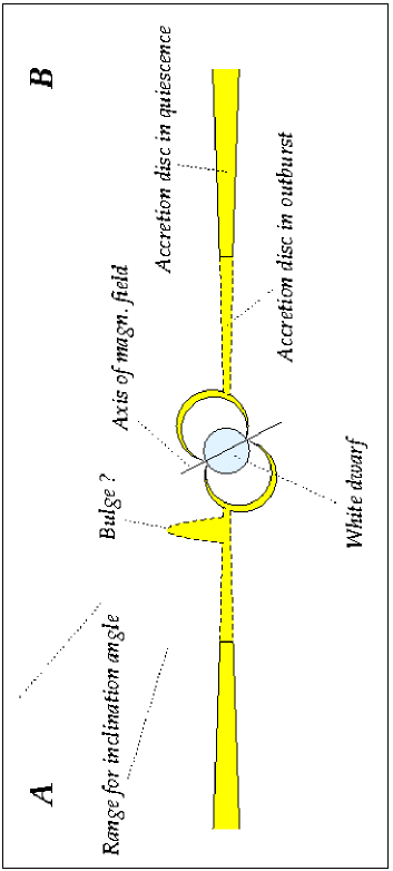
Figure 16: Sketch of GK Per during outburst with cut through the white dwarf, the accretion curtains and the accretion disc.

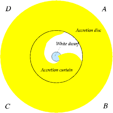
Figure 17: Sketch of the accretion disc and proposed shape of the accretion curtain during outburst in GK Per with accretion disc seen face-on.

7.1 The model

Fig. 16 illustrates our model for GK Per, similar to that proposed by Hellier et al. (2004). During an outburst the inner disc radius shrinks to a few white dwarf radii leading to much shorter accretion curtains. With an inclination angle of $50^{\circ}$ to $73^{\circ}$, the lower pole becomes obscured, reflected in the change from a double peaked spin light curve during quiescence to a single peaked one during outburst. The bulge rotating at the inner disc edge does not only obscure and absorb the X-ray from the accretion region on the white dwarf (Hellier et al. 2004), but also reprocesses the radiation and emits it at UV wavelengths leading to maxima in UV at times the bulge rotates into view (Fig. 6). The optical emission follows probably the UV (QPO) light curve (as Mauche & Robinson 2001 find correlated UV and optical DNOs for SS Cyg).

7.2 Asymmetry of accretion curtains

The variation in the X-ray spin light curve is caused by absorption effects alone (Hellier et al. 2004), i.e., during low phase the pole is pointing towards the observer, causing absorption of the X-ray flux in the accretion column. Thus, a reappearance slower than disappearance of the accretion column indicates that the curtains are asymmetric, spread out and semi-transparent to the X-ray emission from the foot point of the accretion column (see Fig. 16). The fact that the difference in X-ray spectra during spin high and low phase can be solely explained by a variation in the column density supports this model.

Fig. 17 shows a sketch of the model as seen from the ‘north’ pole (accretion disc face-on) and where the southern accretion curtain is left out for clarity of the sketch. During the orbit, the observer views the system clockwise from positions A to D. The shape of the accretion curtain is inspired by the asymmetric spin light curve with a sudden drop (leading bow of the accretion curtain at phase 0.6 in Fig. 5, with observer being at a position between A and B) and slow rise (feathered out accretion curtain wrapped nearly around the white dwarf, phase 0.9 to 1.3, position B to D) and a short maximum (phase 0.3 to 0.5, position D to A) during which we have an essentially undisturbed view of the accretion region and the post-shock part of the accretion column. The shape is caused by the spinning white dwarf dragging material from the inner edge of the accretion disc. Thus, accretion takes place from nearly all azimuths as proposed by Hellier et al. (2004).

7.3 Blobby accretion

The flares are interpreted as an indirect indication of blobby accretion. A somewhat larger accumulation of material (a blob) does not change the light curve if the total amount of accreted material is constant in time. However, if such a large blob enters the photosphere of the white dwarf it leads to enhanced thermal emission at this spot compared to more homogeneously accreted material, as it will penetrate into deeper layers causing a larger surface area of the white dwarf to be affected.

The fact that the flares seem to occur at times when the 5000 s (QPO) cycle shows a maximum is not coincidence if one considers that not only the continous emission from the accretion column but also the flared emission underlies the cyclic variation in the strength of the absorbtion by the rotating bulge.

7.4 The leaky absorber

The simple leaky absorber model describes the hard X-ray part of the observed medium-resolution X-ray emission of the accretion region very well both in quiescence and outburst. The main difference between the outburst and quiescent state is the increased absorption due to larger column densities during quiescence as well as steeply decreased electron $n_{e}$ and ion densities $n_{I}$ due to the enlarged curtains in quiescence. In reality, we are likely to face a more complex physical situation with a range of column densities or variable covering factors (Hellier et al. 1996) due to inhomogeneous in-falling material that would leave too many free parameters to fit for the currently available data.

7.5 Origin of emission lines

The constancy of the emission lines including the Fe fluorescence line with spin period implies that the emission site of these lines are visible at all times and from all viewing angles during an orbit, i.e., it ought to be in the accretion curtain. The Fe fluorescence will also have a contribution from the white dwarf as it possibly shows Compton scattering in the red line wing. Since we do not observe any noticeable line shifts, the accretion curtains must be broad (due to the assumed geometry with a spinning white dwarf and a small inner disc radius) or accretion takes place from all azimuths because during outburst the accretion flow overwhelms the magnetosphere as suggested already by Hellier et al. (2004) or due to the above mentioned scenario.

The fact that the emission lines do also show no variation during the 5000 s (QPO) cycle (flares) implies that their emission site cannot be obscured by the bulge. This is in accordance with the finding that the hard X-ray component shows less variation than the soft component, i.e., they originate in the broad accretion curtains, and with the model of accretion from all azimuths. This again is supported by the width of the emission lines, which are significantly broader than the instrumental broadening (Section 5.1). The increasing width of the lines with wavelength indicates a roughly constant velocity dispersion for all lines, i.e., all lines originate from all parts of the accretion curtain. However, the accretion curtains may be structured and asymmetric as the multi-peaked emission line profiles (especially N vii) suggest.

The shell emission can be fully explained by line emission from ions of, e.g., O, N and Ne. We confirm Balman’s (2001) suggestion that the line emission is produced in the clumped ejecta in the post-shock region, as the shell velocity of $\sim$ 1100 km s^-1 (shell extension of 50″ 99 years after the nova outburst at a distance of 460 pc) results in a too high shock temperature to produce the observed lines.

- (1) Anupama, G.C., Kantharia, N.G. 2005, A&A, in press, astro-ph/0502009
- (2) Arnaud, M. & Raymond, J. 1992, ApJ, 398, 394
- (3) Balman, Ş. 2001, in X-ray Astronomy 2000, ed. R. Giacconi, S. Serio, L. Stella, ASP Conf. Ser., Vol. 234, p.269
- (4) Balman, Ş. 2002a, in The Physics of Cataclysmic Variables and Related Objects, ed. B.T. Gänsicke, K. Beuermann, K. Reinsch, ASP Conf. Ser., 261, 617
- (5) Balman, Ş. 2002b, in The High Energy Universe at Sharp Focus: Chandra Science, ed. by E.M. Schlegel, S.D. Vrtilek, ASP Conf. Ser., 262, 253
- (6) Balman, Ş. 2005, ApJ, in press, astro-ph/0503131
- (7) Balman, Ş. & Ögelman, H.B. 1999, ApJ, 518, L111
- (8) Bhatia, A.K. & Doschek, G.A. 1992, At. Data Nucl. Data Tables, 52, 1
- (9) Brown, G.V., Beiersdorfer, P., Liedahl, D.A., et al. 1998, ApJ, 502, 1015
- (10) Dougherty, S.M., Waters, L.B.F.M., Bode, M.F., Lloyd, H.M., Kester, D.J.M., Bontekoe, Tj.R. 1996, A&A, 306, 547
- (11) Duerbeck, H.W. 1981, PASP, 93, 165
- (12) Evans, A., Bode, M. F., Duerbeck, H. W., Seitter, W. C. 1992, MNRAS, 258, 7
- (13) Frank, J., King, A., Raine D. 1992, Accretion Power in Astrophysics, Cambridge Astrophysics Series, Cambridge University Press
- (14) Hale, G.E. 1901, ApJ, 13, 173
- (15) Hellier, C., Mukai, K. 2004, MNRAS, 352, 1037
- (16) Hellier, C., Harmer, S., Beadmore, A.P. 2004, MNRAS, 349, 710
- (17) Hellier, C., Mukai, K., Ishida, M., Fujimoto, R. 1996, MNRAS, 280, 877
- (18) Gabriel, A.H. & Jordan, C. 1969, MNRAS, 145, 241
- (19) Ishida, M., Sakao, T., Makishima, K., Ohashi, T., Watson, M.G., Norton, A.J., Kawada, M., Koyama, K. 1992, MNRAS, 254, 647
- (20) Kaastra, J. & Mewe, R. 1995, A&AL, 302, L13
- (21) King, A.R. 1995, in Cape Workshop on Magnetic Cataclysmic Variables, ed. D.A.H. Buckley, B. Warner, ASP Conf. Ser., 85, 21
- (22) Mauche, C.W. 2004, in Magnetic Cataclysmic Variables, IAU Coll. 190, ed. S. Vrielmann, M. Cropper, ASP Conf. Ser., 315, 120
- (23) Mauche, C.W., Robinson, E.L. 2001, ApJ, 562, 508
- (24) Mewe, R., Raassen, A.J.J., Drake, J.J., et al. 2001, A&A, 368, 888
- (25) Ness, J.-U., Mewe, R., Schmitt, J.H.M.M., et al. 2001, A&A, 367, 282
- (26) Ness, J.-U. & Wichmann, R. 2002, AN, 323, 129
- (27) Ness, J.-U., Güdel, M., Schmitt, J.H.M.M., et al. 2004, A&A, 427, 667
- (28) McLaughlin, D.B. 1960, in “Stars and Stellar Systems”, Vol. 6 “Stellar Atmospheres”, ed- J.L. Greenstein, Univ. of Chicago Press, Chicago, p. 585
- (29) Morales Rueda, L., Still, M.D., Roche, P. 1996, MNRAS, 283, L58
- (30) Morales Rueda, L., Still, M.D., Roche, P. 1999, MNRAS, 306, 753
- (31) Morales Rueda, L., Still, M.D., Roche, P., Wood, J.H., Lockley, J.J. 2002, MNRAS, 329, 597
- (32) Nogami, D., Kato, T., Baba, H. 2002, PASJ, 54, 987
- (33) Norton, A.J., Watson, M.G., King, A.R. 1988, MNRAS, 231, 783
- (34) Patterson, J. 1991, PASP, 103, 1149
- (35) Pickering, E.C. 1901, ApJ, 13, 170
- (36) Šimon, V. 2002, A&A, 382, 910
- (37) van Teeseling, A., Kaastra, J.S., Heise, J. 1996, A&A, 312, 186
- (38) Warner, B. 1995, “Cataclysmic variable stars”, Cambridge Astrophysics Series, Cambridge University Press, p. 207
- (39) Warner, B., Woudt, P.A. 2002, MNRAS, 335, 84
- (40) Warner, B. 1976, in IAU Symp. 73, “Structure and Evolution of Close Binary Stars”, ed. P. Eggelton, S. Mitton, J. Whelan, Reidel Publishing, Dordrecht), p. 85
- (41) Watson, M.G., King, A.R., Osborne, J. 1985, MNRAS, 212, 917
- (42) Wu, C.-C., Panek, R.J., Holm, A.V., Raymond, J.C., Hartmann, L.W., Swank, J.H. 1989, ApJ, 339, 443
- (43) Yi, I., Kenyon, S.J. 1997, ApJ, 477, 379
- (44) Yi, I., Kim, S.-W., Vishniac, E.T., Wheeler, J.C. 1992, ApJ, 391, L25