Similarity theory of stellar models and structure of very massive stars

Abstract

The similarity theory of stellar structure is used to study the properties of very massive stars when one can neglect all the sources of opacity except for the Thomson scattering. The dimensionless internal structure of such stars is practically independent of the energy generation law. It is shown that the mass-luminosity relation can be approximated by an analytical expression which is virtually universal regarding the chemical composition and energy generation law. A detailed comparison with the Eddington standard model is given. The application of the obtained results to the observations of massive stars is briefly discussed.

¹Max-Planck-Institut für Astrophysik, Garching, Germany
²A.I. Alikhanov Institute for Theoretical and Experimental Physics, Moscow, Russia

1 Introduction

The similarity theory of stellar structure was a powerful tool to understand the properties of stellar models during the pre-computer era of their study. Suffice it to mention a theoretical explanation of the mass-luminosity and mass-radius relations (Biermann, 1931; Strömgren, 1936; Sedov, 1959). For years the similarity theory remains to be useful for the interpretation of various aspects of stellar structure (Schwarzschild, 1958; Chiu, 1968; Cox, Guili, 1968; Dibai, Kaplan, 1976; Kippenhahn, Weigert, 1990).

Here, first we describe the similarity theory of stellar structure as a boundary-value problem formulated by Imshennik and Nadyozhin (1968). Then we discuss the structure of chemically homogeneous stars of so large a mass that the opacity can be considered as being due to the Thomson scattering alone. Such an approximation is believed to be adequate for still hypothetical Pop III stars and for a number of observed luminous stars — e.g., massive O-stars, Wolf-Rayet stars, and some specific stars like $\eta\,$Car, and the Pistol star. A special consideration is given to the comparison with the Eddington standard model.

2 Similarity theory of stellar models

Let us consider a spherical star in hydrostatic and thermal equilibrium. If the pressure $P$ is contributed by perfect gas $P_{\mathrm{g}}$ and black body radiation $P_{\mathrm{r}}$ and the rate of energy generation $\varepsilon$ and opacity $\kappa$ are the power functions of the temperature $T$ and density $\rho$ then the structure of the star is described by the following set of differential equations:

$$\frac{dP}{dr}=-\rho\,\frac{Gm}{r^{2}}\,,$$ (1)

$$\frac{dm}{dr}=4\pi r^{2}\rho\,,$$ (2)

$$\frac{dL}{dr}=4\pi r^{2}\rho\,\varepsilon\,,$$ (3)

$$\frac{dT}{dr}=\left\{\parbox{284.52756pt}{ $-\mbox{$\frac{\raisebox{0.60275pt}{$\textstyle\rho\,T$}}{\raisebox{-2.1097pt}{$\textstyle P$}}$}\mbox{$\frac{\raisebox{0.60275pt}{$\textstyle Gm$}}{\raisebox{-2.1097pt}{$\textstyle r^{2}$}}$}\,\nabla_{A}\,$, \quad$\nabla_{r}\geqslant\nabla_{A}\,,\quad\nabla_{A}=\left(\mbox{$\frac{\raisebox{0.60275pt}{$\textstyle\partial\log T$}}{\raisebox{-2.1097pt}{$\textstyle\partial\log P$}}$}\right)_{S}$ ,\\ $-\mbox{$\frac{\raisebox{0.60275pt}{$\textstyle\rho\,T$}}{\raisebox{-2.1097pt}{$\textstyle P$}}$}\mbox{$\frac{\raisebox{0.60275pt}{$\textstyle Gm$}}{\raisebox{-2.1097pt}{$\textstyle r^{2}$}}$}\,\nabla_{r}\,$, \quad$\nabla_{r}\leqslant\nabla_{A}\,,\quad\nabla_{r}=\mbox{$\frac{\raisebox{0.60275pt}{$\textstyle 3\kappa LP$}}{\raisebox{-2.1097pt}{$\textstyle 16\pi c\,aT^{4}\,Gm$}}$}$\, ,}\right.$$ (4)

$$P=P_{\mathrm{g}}+P_{\mathrm{r}}=\frac{k}{\mbox{$m_{\mathrm{u}}$}}\frac{1}{\mu}\,\rho\,T+\frac{1}{3}\,aT^{4}\,,$$ (5)

$$\beta=\frac{P_{\mathrm{g}}}{P}\,,\qquad\beta^{-1}=1+\mu\,\frac{a\mbox{$m_{\mathrm{u}}$}}{3k}\,\frac{T^{3}}{\rho},\qquad\nabla_{A}=\frac{2(4-3\beta)}{32-24\beta-3\beta^{2}}\,,$$ (6)

$$\kappa=\kappa_{0}\,\rho^{\alpha}\,T^{-\nu}\,,\quad\varepsilon=\varepsilon_{0}\,\rho^{\delta}\,T^{\eta}\,,$$ (7)

where $\beta$ is the ratio of the gas pressure to the total one; $G$, $k$, and $a$ are the gravitational, Boltzmann, and radiation density constants, respectively; $m_{\mathrm{u}}$ is the atomic mass unit and $c$ is the speed of light. The mean molecular mass $\mu$ and the coefficients $\kappa_{0}$ and $\varepsilon_{0}$ depend on composition.

The above equations should meet the boundary conditions:

$$\mbox{Center}\,\quad r=0\,: \qquad m=0\,,\;\;L=0\,,$$ (8)

$$\mbox{Surface}\quad r=R: \qquad P=0\,,\;\;\rho=0\,,\;\;m=M\,.$$ (9)

The conditions (8) tell that there is neither point mass nor point source of energy in the center of the star. The conditions (9) at stellar surface state that both the pressure and density vanish there and the mass $m$ must be equal to the total mass $M$ specified for the star. The stellar radius $R$ is to be obtained as a result of the solution of Eqs. (1)–(7), i.e. $R$ is an eigenvalue of the problem. Simultaneously, the solution gives the luminosity of the star $L_{0}\equiv L(R)$.

Assuming that the chemical composition and, consequently, $\mu$, $\kappa_{0}$, and $\varepsilon_{0}$ are constant throughout the star, one can reduce the above equations to a dimensionless form by measuring the physical quantities in the following set of units (Schwarzschild, 1958):

$$r\;\rightarrow\;R\,,\qquad m\;\rightarrow\;M\,,\qquad L\;\rightarrow\;L_{0}\,,$$

(10)

$$T\,\rightarrow\,\mu\frac{\mbox{$m_{\mathrm{u}}$}}{k}\frac{GM}{R}\equiv T_{0}\,,\quad P\,\rightarrow\,\frac{GM^{2}}{4\pi R^{4}}\equiv P_{0}\,,\quad\rho\,\rightarrow\,\frac{M}{4\pi R^{3}}\equiv\rho_{0}\,.$$

Introducing the following dimensionless variables

$$\mbox{$\!\!\!$}x=r/R,\quad\!q=m/M,\quad\!l=L/L_{0},\quad\!p=P/P_{0},\quad\!\sigma=\rho/\rho_{0},\quad\!t=T/T_{0}\,,$$ (11)

one can rewrite Eqs. (1)–(9) in the form (Imshennik, Nadyozhin, 1968):

$$\frac{dp}{dx}=-\frac{\sigma q}{x^{2}}\,,$$ (12)

$$\frac{dq}{dx}=x^{2}\sigma\,,$$ (13)

$$\frac{dl}{dx}=C_{1}\,x^{2}\sigma^{1+\delta}t^{\eta}\,,$$ (14)

$$\frac{dt}{dx}=\left\{\parbox{284.52756pt}{$-\mbox{$\frac{\raisebox{0.60275pt}{$\textstyle q\sigma t$}}{\raisebox{-2.1097pt}{$\textstyle x^{2}p$}}$}\,\nabla_{A}\,$, \quad$\nabla_{r}\geqslant\nabla_{A}\,$ ,\quad$\nabla_{A}(\beta)=\mbox{$\frac{\raisebox{0.60275pt}{$\textstyle 2(4-3\beta)$}}{\raisebox{-2.1097pt}{$\textstyle 32-24\beta-3\beta^{2}$}}$}\,$,\\ $-\mbox{$\frac{\raisebox{0.60275pt}{$\textstyle q\sigma t$}}{\raisebox{-2.1097pt}{$\textstyle x^{2}p$}}$}\,\nabla_{r}\,$, \quad$\nabla_{r}\leqslant\nabla_{A}\,$, \quad$\nabla_{r}=C_{2}\,\mbox{$\frac{\raisebox{0.60275pt}{$\textstyle p\,l\,\sigma^{\alpha}$}}{\raisebox{-2.1097pt}{$\textstyle q\,t^{4+\nu}$}}$}\,$, }\right.$$ (15)

$$p=\sigma t+B\,t^{4}\,,\qquad\beta^{-1}=1+B\,\frac{t^{3}}{\sigma}\,,$$ (16)

where all the parameters are gathered in the three dimensionless constants:

$$C_{1} = \frac{1}{(4\pi)^{\delta}}\left(\frac{G\mbox{$m_{\mathrm{u}}$}}{k}\right)^{\eta}\mu^{\eta}M^{1+\delta+\eta}\;\frac{\varepsilon_{0}}{L_{0}R^{3\delta+\eta}}\,,$$ (17)

$$C_{2} = \frac{3\,(4\pi)^{-\alpha}}{64\pi^{2}\,ac}\left(\frac{k}{G\mbox{$m_{\mathrm{u}}$}}\right)^{4+\nu}\mu^{-4-\nu}M^{\alpha-3-\nu}\frac{\kappa_{0}L_{0}}{R^{3\alpha-\nu}}\,,$$ (18)

$$B = \frac{4\pi a}{3G}\left(\frac{G\mbox{$m_{\mathrm{u}}$}}{k}\right)^{4}\left(\mu^{2}M\right)^{2}\,=\,0.78096\left(\mu^{2}M/\mbox{$M_{\textstyle\odot}\,$}\right)^{2}.$$ (19)

The dimensionless boundary conditions become:

$$\mbox{Center $\;x=0$}:\quad q=0\,,\;\;l=0\,,$$ (20)

$$\mbox{Surface $x=1$}:\quad p=0\,,\;\;t=0\,,\;\;l=1\,,\;\;q=1\,.$$ (21)

Thus, we have now six boundary conditions for four first order differential equations (12)–(15). This means that for every given $B$ (or $\mu^{2}M$) the constants $C_{1}$ and $C_{2}$ can have only quite certain values (eigenvalues) in order that the solution of four differential equations would satisfy to six boundary conditions. The solution itself as well as $C_{1}$ and $C_{2}$ depend only on $\mu^{2}M$ and the exponents $\alpha$, $\nu$, $\delta$, $\eta$: $C_{1,2}=C_{1,2}(\mu^{2}M,\alpha,\nu,\delta,\eta)$.

Equations (12)–(16) can be solved by standard methods. For the calculations described in the next section, we have used the following approach. Having chosen some trial values of $C_{1}$ and $C_{2}$ and integrating Eqs. (12)–(16) numerically from the surface [$x=1$, boundary conditions (21)] inward to some value $x=x_{f}$ $(0<x_{f}<1)$, one obtains a set of four quantities $\left\{p(x_{f}),q(x_{f}),l(x_{f}),t(x_{f})\right\}$ as functions of $C_{1}$ and $C_{2}$. Then integrating these equations again from the center [$x=0$, boundary conditions (20)] with the same $C_{1}$ and $C_{2}$ and trial values $p(0)=p_{c}$ and $t(0)=t_{c}$ outward to $x_{f}$ one obtains a similar set of quantities that depends now on $C_{1}$, $C_{2}$, $p_{c}$, and $t_{c}$. Since $p(x)$, $q(x)$, $l(x)$, and $t(x)$ must be continuous throughout the star, both the sets have to coincide at $x=x_{f}$. One can organize an iterative process for four unknown parameters $C_{1}$, $C_{2}$, $p_{c}$, and $t_{c}$ to find such their values that would ensure the desired continuity of four variables $p$, $q$, $l$, and $t$ at $x=x_{f}$. Of course, the result does not depend on $x_{f}$ but the convergence domain of the iterations does.

As soon as $C_{1}$ and $C_{2}$ are found, one can easily derive the luminosity $L_{0}$ and radius $R$ from Eqs.  (17) and (18) which represent the mass-radius and mass-luminosity relation, respectively.

3 Structure of very massive stars

In this section, the above similarity theory is employed to describe the structure of very massive stars. In this case the opacity is dominated by the Thomson scattering and one can assume $\alpha=0$, $\nu=0$, and $\kappa=\kappa_{0}=0.2(1+\mathrm{X})\;$cm²/g (X is the mass fraction of hydrogen).

The mass-luminosity relation [Eq. (18)] can be converted into the form

$$L_{0}\,=\,\frac{64\pi^{2}\,ac}{3\,\kappa_{0}}\left(\frac{G\mbox{$m_{\mathrm{u}}$}}{k}\right)^{4}\mu^{4}\,M^{3}\,C_{2}(\mu^{2}M,\delta,\eta)\,.$$ (22)

All the models with physically reasonable values of the energy generation temperature exponent (i.e., $\eta\geqslant 4$) considered below have convective cores and radiative outer envelopes. Using Eqs. (12) and (15) and boundary conditions (21), one can find that $C_{2}$ is simply connected with $\beta_{\mathrm{s}}(\mu^{2}M,\delta,\eta)$ — the value of the parameter $\beta$ at stellar surface:

$$1-\beta_{\mathrm{s}}\,=\,4\,B\,C_{2}\,.$$ (23)

Now the mass-luminosity relation can be reduced to

$$L_{0}\,=\,L_{\mathrm{Ed}}(1-\beta_{\mathrm{s}})\,,$$ (24)

where the Eddington critical luminosity $L_{\mathrm{Ed}}$ is given by

$$L_{\mathrm{Ed}}\,\equiv\,\frac{4\pi cGM}{\kappa_{0}}\,=\,\frac{\mbox{$6.483\!\times\!10^{4}\,$}}{1+\mbox{X}}\frac{M}{\mbox{$M_{\textstyle\odot}\,$}}\,\mbox{$L_{\textstyle\odot}$}\,.$$ (25)

Using the Runge–Kutta method with automatic control of accuracy for solving Eqs. (12)–(16) from stellar surface down to $x_{f}$ and from center up to $x_{f}$, we have calculated a large number of models for a wide interval of the parameter $\mu^{2}M$ $(0\leqslant\mu^{2}M\leqslant\mbox{$4,000\,M_{\textstyle\odot}$})$. Typically, the values $x_{f}\approx 0.1-0.3$ are the best for the iterations to converge. The convergence domain, however, turned out to be rather narrow at least for the Newton–Raphson iteration scheme used in our calculations. So, when calculating a sequence of such models one has to change $\mu^{2}M$ at most by a few percents in order to ensure the convergence.

Table 1 presents the most important properties of several selected models. Note that for the sake of a better perception we use hereafter for dimensionless quantities the same designations as for dimensional ones. The first row of Table 1 gives $\mu^{2}M$ with M measured in $M_{\textstyle\odot}\,$. The next three rows are the $C_{1}$-values for three modes of energy generation: the CNO-cycle, $3\alpha$-reaction, and pp-chain. The fifth row gives the $C_{2}$-values. The next six rows relate to the central dimensionless values of density $\rho_{\mathrm{c}}$, pressure $P_{\mathrm{c}}$, temperature $T_{\mathrm{c}}$, radiative temperature gradient $\nabla_{r\mathrm{c}}$, gravitational potential $\varphi_{\mathrm{c}}$ (in the units $GM/R$), and ratio $\beta_{\mathrm{c}}$ of the gas pressure to the total one. The next two rows contain $\beta_{\mathrm{conv}}$ and $\beta_{\mathrm{s}}$ at the convective core boundary and at stellar surface, respectively. Finally, the last six rows present the dimensionless values of radius, mass, luminosity, density, pressure, and temperature at the convective core boundary.

Table 1: Structural properties of selected models

$\mu^{2}M$	0	10	30	100	300	1000	4000
$\log_{10}C_{1}\,^{\star}$	1.6347	3.4318	5.8102	8.8083	11.768	15.281	19.622
$\log_{10}C_{1}\,^{\dagger}$	2.1212	5.8346	10.615	16.602	22.509	29.523	38.199
$\log_{10}C_{1}\,^{\spadesuit}$	-0.4145	0.0220	0.5988	1.2961	1.9789	2.8051	3.8511
$\log_{10}C_{2}$	-3.2981	-3.5181	-3.9842	-4.7533	-5.5839	-6.5626	-7.7304
$\rho_{\mathrm{c}}$	59.34	60.20	65.05	79.97	98.95	119.4	137.5
$P_{\mathrm{c}}$	45.55	43.95	46.43	58.41	75.32	94.78	112.8
$T_{\mathrm{c}}$	0.7677	0.5816	0.4097	0.2630	0.1699	0.1014	0.0539
$\nabla_{r\mathrm{c}}\,^{\star}$	2.459	3.249	4.525	5.806	6.588	6.992	7.266
$\varphi_{\mathrm{c}}$	-3.428	-3.389	-3.421	-3.602	-3.821	-4.034	-4.204
$\beta_{\mathrm{c}}$	1	0.7967	0.5739	0.3601	0.2232	0.1278	0.0657
$\beta_{\mathrm{conv}}$	1	0.8671	0.6689	0.4294	0.2600	0.1429	0.0704
$\beta_{\mathrm{s}}$	1	0.9053	0.7085	0.4489	0.2673	0.1451	0.0709
$r_{\mathrm{conv}}$	0.2832	0.3903	0.5107	0.6264	0.7077	0.7771	0.8380
$m_{\mathrm{conv}}$	0.3120	0.5691	0.8063	0.9412	0.9823	0.99531	0.99895
${L_{\mathrm{conv}}}^{\spadesuit}$	0.7810	0.9799	0.9991	1.0000	1.0000	1.0000	1.0000
$\rho_{\mathrm{conv}}$	31.39	16.02	5.985	1.661	0.5056	0.1429	0.0379
$P_{\mathrm{conv}}$	15.76	5.830	1.446	0.2540	0.05324	0.01049	0.00184
$T_{\mathrm{conv}}$	0.5022	0.3157	0.1616	0.06564	0.02736	0.01036	0.00342
${}^{\star}\,$CNO-cycle $(\delta=1,\,\eta=16)$,  ${}^{\dagger}\,$$3\alpha$-reaction $(\delta=2,\,\eta=30)$,  ${}^{\spadesuit}\,$pp-chain $(\delta=1,\,\eta=4)$

The calculated sequences of one-parametric (depending on $\mu^{2}M$) dimensionless models have so large convective cores that the major part of thermonuclear energy turns out to be released within the core. Therefore, $L(r)$ becomes almost equal to the luminosity $L_{0}$ everywhere outside the convective core. For such a strong dependence of the energy generation on temperature as in the CNO-cycle $(\eta=16)$ and in $3\alpha$-reaction $(\eta=30)$, one can with a high accuracy assume $l(x)=1$ in Eq. (15). Consequently, Eq. (14) for $l(x)$ proves to be disentangled from other equations (12), (13), (15), and (16). Now one can calculate the overall stellar structure by solving a truncated eigenvalue problem that pays no attention to the law of energy generation and considers the constant $C_{2}$ as a single eigenvalue parameter involved. In particular, the resulting $C_{2}$-eigenvalue, and consequently $L_{0}$ [Eq. (22)], as well as the dimensionless stellar structure do not depend on the exponents $\delta$ and $\eta$. Such a truncated model is actually the point-source model with the Thomson opacity and allowance for the radiation pressure that was first calculated by Henrich (1943) within a limited range of stellar mass $(0\leqslant\mu^{2}M\leqslant 119)$. Our numerical results are in excellent agreement with his $\sim 1$% accurate calculations.

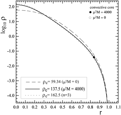
Figure 1: Density versus radius in the units defined by Eqs. (10) for $\mu^{2}M=0$ (dashed line), 4000 (full line) and for a polytropic model ($n=3$, dotted line). The boundaries of the convective core are indicated for $\mu^{2}M=0\mbox{ and }4000$.

When $C_{2}$ and the dimensionless functions $\sigma(x)$ and $t(x)$ are already known from the solution of the truncated problem one can find the constant $C_{1}$ and spatial distribution of the dimensionless luminosity $l(x)$:

$$C_{1}=\left[\int_{0}^{1}\!x^{2}\,\sigma^{1+\delta}\,t^{\eta}\,{\mathrm{d}}x\right]^{-1},\qquad l(x)=C_{1}\int_{0}^{x}\!x^{2}\,\sigma^{1+\delta}\,t^{\eta}\,{\mathrm{d}}x\,.$$ (26)

If the energy generation is an arbitrary (but still strongly varying with temperature) function: $\varepsilon=\varepsilon(\rho,T)$, then instead of $C_{1}$ one has to consider the stellar radius $R$ as an eigenvalue that can be found from the equation

$$L_{0}\,=\,M\int_{0}^{1}\!x^{2}\,\sigma(x)\;\varepsilon\!\left[\frac{M}{4\pi R^{3}}\sigma(x),\,\mu\frac{\mbox{$m_{\mathrm{u}}$}}{k}\frac{GM}{R}t(x)\right]{\mathrm{d}}x\,,$$ (27)

where for given $M$ and composition the luminosity $L_{0}$ is determined by the $C_{2}$-value obtained for the truncated model.

The structural properties of the models presented in Table 1 correspond to three modes of energy generation: the CNO-cycle, $3\alpha$-reaction, and pp-chain. For the CNO-cycle and $3\alpha$-reaction, the dimensionless luminosity $L_{\mathrm{conv}}$ at the convective core boundary is equal to 1.0000 for all the values of $\mu^{2}M$. The same is true for the pp-chain when $\mu^{2}M\gtrsim 30$. All other parameters in Tables 1 and 2, except for $C_{1}$ and $\nabla_{r\mathrm{c}}$, prove to be the same for the CNO-cycle and $3\alpha$-reaction, and at $\mu^{2}M\gtrsim 30$ for the pp-chain as well. Practically, one can consider only the interval $0\leqslant\mu^{2}M\lesssim 10$ as exhibiting slight differences for the pp-chain shown in Figures 4, 5, 6 below. This concerns also the mass-luminosity relation. More specifically, for $\eta=4$: $\log_{10}C_{2}=-3.516$ and $-3.285$ at $\mu^{2}M=10$ and $0$, respectively.

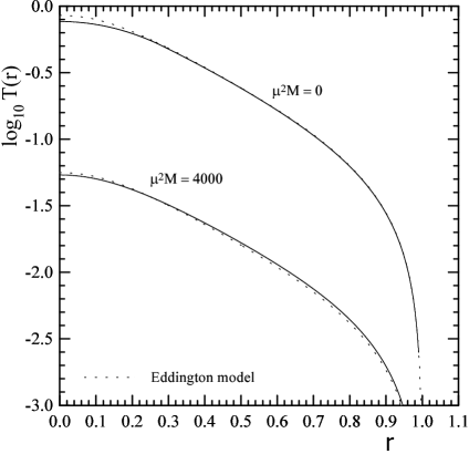
Figure 2: Temperature versus radius in the units defined by Eqs. (10) for $\mu^{2}M=0$ and 4000. The Eddington model is shown by the dotted lines.

The constant $C_{1}$ and central value of the logarithmic radiative temperature gradient $\nabla_{r\mathrm{c}}=C_{1}C_{2}\,p_{\mathrm{c}\,}\sigma_{\mathrm{c}}^{\delta\,}t_{\mathrm{c}}^{\eta-4}$ strongly depend on the energy generation law. The $\nabla_{r\mathrm{c}}$ values for the CNO-cycle in Table 1 demonstrate that even for low masses $(\mu^{2}M\lesssim 1)$ when one can neglect the radiation pressure, there is still a good excess of $\nabla_{r\mathrm{c}}$ over $\nabla_{A}$ $(0.25\leqslant\nabla_{A}\leqslant 0.4)$ to drive the adiabatic convection along stellar core. For the $3\alpha$-reaction, the excess is much larger: $\nabla_{r\mathrm{c}}=11.05$ for $\mu^{2}M=0$. However for the pp-chain we have $\nabla_{r\mathrm{c}}=0.594$ — the value exceeding the adiabatic gradient only by a factor of 1.5 $(\nabla_{A\mathrm{c}}=0.4$ for $\mu^{2}M\approx 0)$. This happens because the exponent $\eta=4$ is not very far from a critical value of $\eta\approx 2-3$ necessary to ensure the existence of the convective core (Cowling, 1934; Naur, Osterbrock, 1953).

Figures 1 and 2 show the density and temperature versus radius for two extreme values of $\mu^{2}M$ in the case of the CNO-cycle and $3\alpha$-reaction. With a high accuracy these two modes of energy generation result in only one model for every given $\mu^{2}M$ (see the discussion above).

It is instructive to compare the results with the Eddington standard model (Eddington, 1926) that at constant opacity corresponds to a constant rate of energy generation: $\varepsilon=\varepsilon_{0}$ $(\eta=0,\,\delta=0)$. In this case $C_{1}=1$ as it immediately follows from Eq. (26). Then, it is easy to make sure that $\beta$ is to be constant inside such a model. As a result, the pressure turns out to be connected with density along the radius by a power law:

$$P\,=\,K\>\rho^{4/3},\qquad K\equiv\frac{k}{m_{{\mbox{\scriptsize u}}}\mu}\left[\frac{3k}{am_{{\mbox{\scriptsize u}}}\mu}\,\frac{1-\beta}{\beta^{4}}\right]^{1/3}=\mbox{ const}\,.$$ (28)

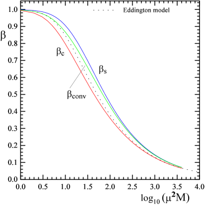
Figure 3: The ratios of the gas pressure to the total one, $\beta$, at the center $\beta_{\mathrm{c}}$, the convective core boundary $\beta_{\mathrm{conv}}$, and the surface $\beta_{\mathrm{s}}$ as functions of $\mu^{2}M$ ($M$ is in $M_{\textstyle\odot}\,$). A dotted curve corresponds to the Eddington standard model [Eq. (29)].

Thus, the standard model is nothing else than a polytropic gas sphere of index $n=3$. The value of $\beta$ proves to be uniquely connected with the mass $M$ by the following equation (Chandrasekhar, 1939):

$$\frac{1-\beta}{\beta^{4}}\,=\,0.01607\,G^{3}\left(\frac{m_{{\mbox{\scriptsize u}}}}{k}\right)^{4}\left(\mu^{2}M\right)^{2}\,=\,\mbox{$2.994\!\times\!10^{-3}\,$}\left(\mu^{2}\frac{M}{\mbox{$M_{\textstyle\odot}\,$}}\right)^{2}\,.$$ (29)

The constant $C_{2}$ as a function of $\mu^{2}M$ and the mass-luminosity relation for the standard model are determined by Eqs. (23) and (24) with $\beta_{\mathrm{s}}$ being substituted for $\beta$ from Eq. (29). It is easy to verify that the Eddington standard model has no convective core at all — it is convectively stable for any $\mu^{2}M$.

According to Fig. 3, $\beta$ increases from the stellar center up to the surface: $\beta_{\mathrm{c}}<\beta_{\mathrm{conv}}<\beta_{\mathrm{s}}$, the Eddington $\beta$ always remaining between $\beta_{\mathrm{c}}$ and $\beta_{\mathrm{conv}}$.

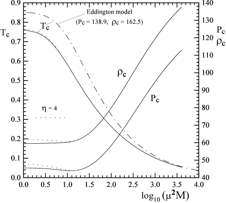
Figure 4: The dimensionless central pressure $P_{\mathrm{c}}$, density $\rho_{\mathrm{c}}$ (right vertical axis), and temperature $T_{\mathrm{c}}$ (left vertical axis) as functions of $\mu^{2}M$ ($M$ is in $M_{\textstyle\odot}\,$).

Figure 4 shows the central pressure $P_{\mathrm{c}}$, density $\rho_{\mathrm{c}}$ and temperature $T_{\mathrm{c}}$ as functions of $\mu^{2}M$. At $\mu^{2}M\lesssim 10$, these quantities for the pp-chain (dotted lines) only slightly differ from those for the CNO-cycle and $3\alpha$-reaction (solid lines). The broken line represents $T_{\mathrm{c}}$ for the Eddington model for which $P_{\mathrm{c}}$ and $\rho_{\mathrm{c}}$ are independent of $\mu^{2}M$: $P_{\mathrm{c}}=138.9$, $\rho_{\mathrm{c}}=162.5$ (polytrope $n=3\,$!).

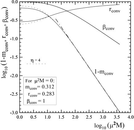
Figure 5: The convective core boundary characteristics as functions of $\mu^{2}M$ for the CNO-cycle and $3\alpha$-reaction (solid lines) and pp-chain (dotted lines). The values for the CNO-cycle and $3\alpha$-reaction at $\mu^{2}M=0$ are shown explicitly.

Figure 5 shows how the dimensionless radius of the convective core $r_{\mathrm{conv}}$, the value of $\beta$ at the convective core boundary $\beta_{\mathrm{conv}}$, and the mass above the convective core $(1-m_{\mathrm{conv}})$ depend on $\mu^{2}M$. At $\mu^{2}M\gtrsim 40$, the convective core contains more than 85% of stellar mass. One can approximate $m_{\mathrm{conv}}$ (for all the three energy generation modes!) by the following asymptotic relation (a straight broken line in Fig. 5):

$$m_{\mathrm{conv}}\,=\,1-9.075\left(\mu^{2}M\right)^{-1.095}\,,\quad\mu^{2}M\gtrsim 40\,.$$ (30)

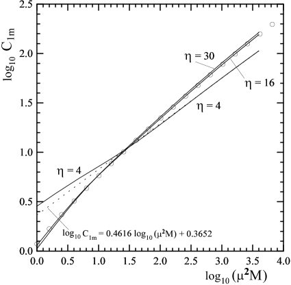
Figure 6: The modified constant $C_{1\mathrm{m}}$ as a function of $\mu^{2}M$ for the CNO-cycle, $3\alpha$-reaction and pp-chain. The open circles and dashed line show polynomial fits.

Since the constant $C_{1}$ strongly depends on the energy generation mode (Table 1), it is useful to introduce a modified constant $C_{1\mathrm{m}}$:

$$C_{1\mathrm{m}}(\mu^{2}M)\,\equiv\,(\mu^{2}M)^{\frac{\delta+\eta}{3\delta+\eta}}\,{\left[\left(1-\beta_{\mathrm{s}}\right)C_{1}\right]^{-\frac{1}{3\delta+\eta}}}\,,\qquad(M\mbox{ in }\mbox{$M_{\textstyle\odot}\,$})\,.$$ (31)

Now, using Eq. (24) for $L_{0}$ we can obtain the following expression for stellar radius as a function of $\mu^{2}M$ and composition:

$$\log R\,=\,\log C_{1\mathrm{m}}\,+\,\log D\,+\,\log S\,,\quad(R\mbox{ in }\mbox{$R_{\textstyle\odot}\,$})\,,$$ (32)

where

$$\log D = \frac{1}{3\delta+\eta}\log[0.2\,(1+X)\,\xi]-\frac{2\delta+\eta}{3\delta+\eta}\log\mu\,,$$

$$\log S = \frac{\eta}{3\delta+\eta}\log\left(\frac{G\mbox{$m_{\mathrm{u}}$}}{k}\right)-\frac{\delta+1}{3\delta+\eta}\log(4\pi)$$

$$+\frac{1}{3\delta+\eta}\log\left(\frac{\varepsilon_{00}}{c\,G}\right)+\frac{\delta+\eta}{3\delta+\eta}\log\mbox{$M_{\textstyle\odot}\,$}\!-\log\mbox{$R_{\textstyle\odot}\,$}\,,$$

$$\xi \equiv \mathrm{X}^{2}\mbox{ \footnotesize(pp-chain), }\;\mathrm{X}\,\mathrm{X}_{\mathrm{CNO}}\mbox{ \footnotesize(CNO-cycle), }\;\mathrm{Y}^{3}\mbox{\footnotesize(3$\alpha$-reaction)}\,.$$

Here, the dependences of $\varepsilon_{0}$ on the mass fractions of hydrogen $X$, the CNO-isotopes $\mathrm{X}_{\mathrm{CNO}}$, and helium $Y$ are shown explicitly $(\varepsilon_{0}=\varepsilon_{00}\;\xi)$. For large values of $\eta$, $C_{1\mathrm{m}}$ becomes independent of the energy generation mode — compare the CNO $(\eta=16)$ and $3\alpha$ $(\eta=30)$ curves in Fig. 6. Both the $C_{1\mathrm{m}}$ can be approximated by a single polynomial shown by open circles in Fig. 6:

$$y=0.0720052+0.782547x-0.120854x^{2}+0.0295923x^{3}-0.0030574x^{4}\,,$$ (33)

where $y\equiv\log_{10}C_{1\mathrm{m}}$ and $x\equiv\log_{10}\left(\mu^{2}M\right)$. A fit for the pp-chain $(\eta=4)$ is shown in Fig. 6 by a dashed line that gives a good accuracy for $\mu^{2}M\gtrsim 10$.

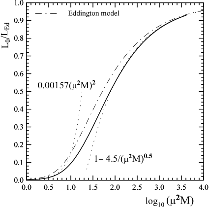
Figure 7: The normalized mass-luminosity relation [Eq. (24)]. Dotted curves indicate asymptotics for small and large $\mu^{2}M$-values. The Eddington model is shown by a broken line.

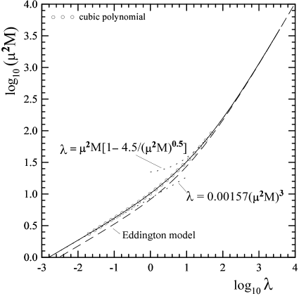
Figure 8: The mass-luminosity relation ($M$ in $M_{\textstyle\odot}\,$, see text).

Figure 7 shows luminosity $L_{0}$ in terms of $L_{\mathrm{Ed}}$ as a function of $\mu^{2}M$ [solid curve specified by Eq. (24)]. The curve virtually holds for all the three energy generation modes — a small difference for the pp-chain at $\mu^{2}M<10$ is indistinguishable on the scale of the figure. For given $\mu^{2}M$, the Eddington model is always over-luminous (by a factor of two at $\mu^{2}M<10$).

For the sake of practical use, it is worth to rewrite the mass-luminosity relation in terms of variable $\lambda$:

$$\lambda\,\equiv\,\mu^{2}\frac{M}{\mbox{$M_{\textstyle\odot}\,$}}\,\frac{L_{0}}{L_{\mathrm{Ed}}}\,=\,\frac{\mu^{2}\kappa_{0}L_{0}}{4\pi cG\mbox{$M_{\textstyle\odot}\,$}}=\mbox{$1.5426\!\times\!10^{-5}\,$}\mu^{2}(1+\mbox{X})\frac{L_{0}}{\mbox{$L_{\textstyle\odot}$}}\,,$$ (34)

Connecting the asymptotics for small and large $\mu^{2}M$-values by a cubic spline that ensures the continuity of the function and its first derivatives (open circles in Fig. 8) one obtains the following analytical approximation:

$$\lg(\mu^{2}M) \!\!\!\!=\!\!\!\! 0.9347\,+\,\frac{1}{3}\lg\lambda\,,\qquad\qquad\qquad\qquad\qquad\quad(\lg\lambda\leqslant-1.7),$$

$$\lg(\mu^{2}M) \!\!\!\!=\!\!\!\! 1.015209+0.449843\lg\lambda+0.0534969\lg^{2}\lambda$$

$$+\,0.00754094\lg^{3}\lambda\,,\!\qquad\qquad\qquad\quad\;\;(-1.7<\lg\lambda<1.7),$$

$$\mu^{2}M \!\!\!\!=\!\!\!\! 10.125\left(1+0.0987654\lambda+\sqrt{1+0.1975\lambda}\right),\;\;\;(\lg\lambda\geqslant 1.7).$$

Table 2: Integral properties of selected models

$\mu^{2}M$​​	0	10	30	100	300	1000	4000	Edd
$E_{\mathrm{g}}\,^{\ast}$​​	-1.227	-1.206	-1.205	-1.254	-1.318	-1.383	-1.435	-1.5
$E_{\mathrm{T}}$​​	0.6137	0.6969	0.8350	1.016	1.166	1.292	1.387	1.450
$I\,^{\dagger}$​​	0.1561	0.1616	0.1630	0.1536	0.1412	0.1302	0.1222	0.113
$I_{\mathrm{conv}}$​​	0.0139	0.0439	0.0908	0.1247	0.1309	0.1271	0.1214	—
$t_{\mathrm{s}}$​​	2.438	2.517	2.580	2.624	2.649	2.665	2.677	2.723
$t_{\mathrm{conv}}$​​	0.269	0.433	0.619	0.843	1.044	1.251	1.472	—
$\tau_{\mathrm{c}}$​​	1.441	1.426	1.475	1.664	1.896	2.132	2.329	2.587
$\langle\gamma\rangle$​​	5/3	1.532	1.453	1.401	1.3733	1.3555	1.3445	1.345
$\omega$​​	2.804	2.109	1.629	1.288	1.058	0.840	0.627	0.667
∗ $E_{\mathrm{g}}$ attains a maximum $-1.2005$ at $\mu^{2}M=18.5$
† $I$ attains a maximum $0.1636$ at $\mu^{2}M=21$

Equation (3) allows to estimate $M$ when the luminosity $L_{0}$ and the representatives of composition ($\mu$ and $X$) are known. On the contrary, in order to estimate $L_{0}$ for given $M$ and composition one can either solve Eq. (3) for $\lambda$ or use the following accurate approximation:

$$\lambda \!\!\!\!=\!\!\!\! 0.00157\left(\mu^{2}M\right)^{3},\qquad\qquad\qquad\qquad\qquad\quad\quad\left(\mu^{2}M\leqslant 2.4\right),$$

$$\lg\lambda \!\!\!\!=\!\!\!\! -2.907029+3.552793\lg\left(\mu^{2}M\right)-0.7717945\lg^{2}\left(\mu^{2}M\right)$$

$$+\,0.078623\lg^{3}\left(\mu^{2}M\right),\!\qquad\qquad\qquad\quad\left(2.4<\mu^{2}M<100\right),$$

$$\lambda \!\!\!\!=\!\!\!\! \mu^{2}M\left(1-\frac{4.5}{\sqrt{\mu^{2}M}}\right),\;\;\;\qquad\qquad\qquad\qquad\quad\left(\mu^{2}M\geqslant 100\right).$$

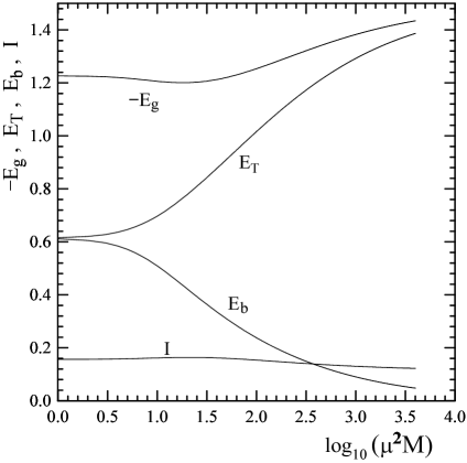
Figure 9: Dimensionless gravitational $E_{\mathrm{g}}$ and thermal $E_{\mathrm{T}}$ energies, central moment of inertia $I$, and gravitational binding energy $E_{\mathrm{b}}$ versus $\mu^{2}M$.

Concluding this section we present in Table 2 a number of integral properties of stellar models such as gravitational $E_{\mathrm{g}}$ and thermal $E_{T}$ energies (in units $GM^{2}/R$), central moment of inertia of the whole star $I=\int^{M}_{0}\!r^{2}\,\mathrm{d}m$ and that of the convective core $I_{\mathrm{conv}}$ (in units $MR^{2}$), the time sound takes to propagate from the center up to the surface $t_{\mathrm{s}}=\int^{R}_{0}\!\frac{\mathrm{d}r}{\sqrt{\gamma P/\rho}}$ and to the convective core boundary $t_{\mathrm{conv}}$ (in units $\sqrt{R^{3}/(GM)}\,$), column density of the star $\tau_{\mathrm{c}}=\int^{R}_{0}\!\rho\,\mathrm{d}r$ (in units $M/R^{2}$), average adiabatic index $\langle\gamma\rangle=\frac{\int^{M}_{0}\!\gamma\,(P/\rho)\,\mathrm{d}m}{\int^{M}_{0}\!(P/\rho)\,\mathrm{d}m}$, and an estimate of fundamental angular frequency $\omega=\sqrt{(3\langle\gamma\rangle-4)|E_{\mathrm{g}}|/I}$ of radial pulsations (in units $\sqrt{GM/R^{3}}\,$).

The last column in Table 2 presents the properties of the Eddington standard model at $\mu^{2}M=4000$. Note that for the standard model the dimensionless $E_{\mathrm{g}}$, $I$ and $\tau_{\mathrm{c}}$ are determined by the polytrope $n=3$ structure and do not depend on $\mu^{2}M$.

Figure 9 shows $E_{\mathrm{g}}$, $E_{\mathrm{T}}$, $I$, and gravitational binding energy $E_{\mathrm{b}}=-E_{\mathrm{tot}}=-(E_{\mathrm{g}}+E_{\mathrm{T}})$ as functions of $\mu^{2}M$.

4 Comparison with detailed models

In order to demonstrate potentialities of the similarity theory we compare our results with detailed models of massive main sequence stars calculated by Schaller et al. (1992) and the models of helium and carbon-oxygen stars (Wolf-Rayet stars) studied by Langer (1989) and Deinzer and Salpeter (1964). Figures 10–13 display such a comparison.

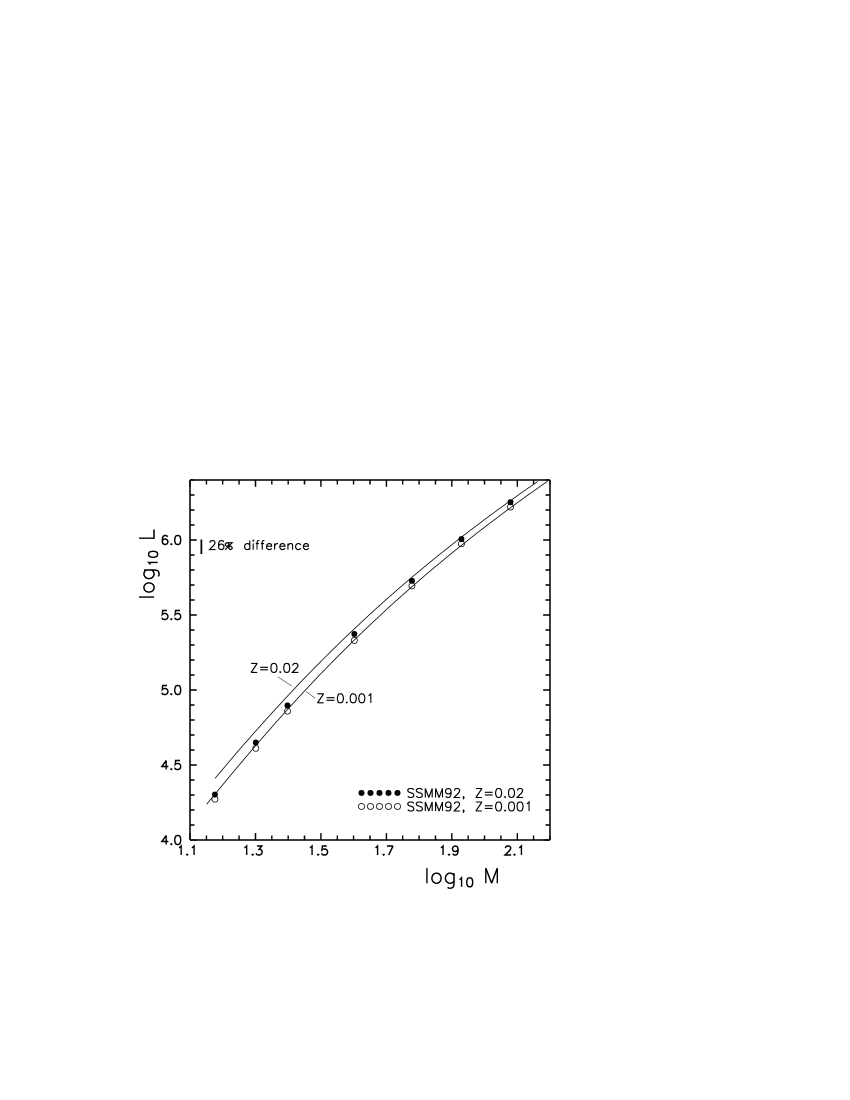
Figure 10: The mass-luminosity relation (solid lines) in comparison with the detailed models of Schaller et al. (1992) (filled and open circles). $M$ and $L$ are in solar units.

Solid curves in Fig. 10 are obtained with the aid of Eq. (3) for two specified by Schaller et al. (1992) compositions: X=0.680, Y=0.300, Z=0.020 (upper curve) and X=0.756, Y=0.243, Z=0.001 (lower curve). One can observe an excellent agreement for low metallicity $(Z=0.001)$ and a fairly good coincidence for $Z=0.02$. In the latter case our models are slightly over-luminous (by 25% at $M=\mbox{$15\,M_{\textstyle\odot}$}$). This natural result can be interpreted as on average a 25% contribution to the opacity coming from sources other than the electron scattering.

Figure 11: The mass-radius relation (solid lines) in comparison with the detailed models of Schaller et al. (1992) (filled and open circles). $M$ and $R$ are in solar units.

The mass-radius relation for the same models is shown in Fig. 11. The detailed models have systematically larger radii (typically by $\sim 5\%$ for Z=0.02) as compared with our models (solid lines). This can be explained by a noticeable increase in opacity in stellar envelope owing to the absorption in atomic spectral lines (Imshennik, Nadyozhin, 1967). The solid lines were calculated with the aid of Eqs. (32) and (33) assuming the CNO-cycle as the main energy source with the energy generation law taken from Caughlan, Fowler (1988) and approximated by

$$\varepsilon_{\mathrm{CNO}}\,=\,\mbox{$8.43\!\times\!10^{-3}\,$}X_{\mathrm{CNO}}X\rho\,T^{16}_{7}\;\mbox{erg$\,$g${}^{-1}$s${}^{-1}$},\quad(2.2\leqslant T_{7}\leqslant 3.6)\,,$$ (37)

where $T_{7}\equiv T/10^{7}\mathrm{K}$ and $\rho$ is in g cm^-3. Within the indicated limits for $T_{7}$, the accuracy of Eq. (37) is better than 10%.

Figure 12: Dimensionless mass of the convective core $m_{\mathrm{conv}}$ and central value of $\beta$ (solid and dashed lines) in comparison with Schaller et al. (1992) (filled and open circles and squares). Solid and dashed lines are for $Z=0.001$ and $Z=0.02$, respectively; $M$ is in $M_{\textstyle\odot}\,$.

Similar approximation for the $3\alpha$-reaction is given by the following power law

$$\varepsilon_{3\alpha}\,=\,\mbox{$4.95\!\times\!10^{-38}\,$}\mathrm{Y}^{3}\rho^{2}\,T^{30}_{7}\;\mbox{erg$\,$g${}^{-1}$s${}^{-1}$},\quad(T_{7}>8)\,.$$ (38)

The accuracy of the approximation is better than 10% at $T_{7}>8$.

The structural properties of our models are also in a good agreement with the detailed models as it is exemplified in Fig. 12 for central value of $\beta$ and the convective core mass fraction $m_{\mathrm{conv}}$.

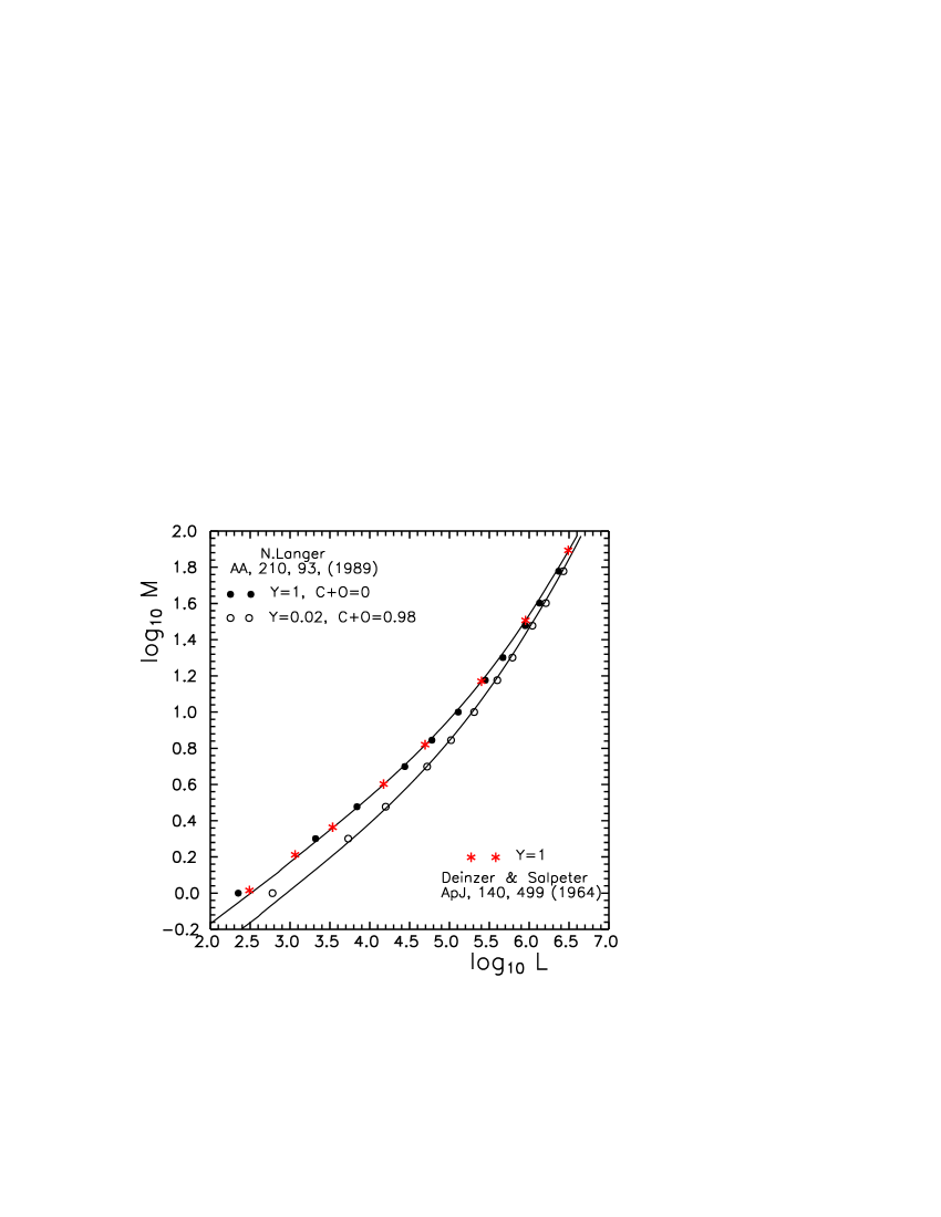
Figure 13: The mass-luminosity relation for the helium and carbon-oxygen Wolf-Rayet stars (solid lines) in comparison with the detailed models of Langer (1989) (filled and open circles) and Deinzer and Salpeter (1964) (asterisks). $M$ and $L$ are in solar units.

Figure 13 shows the mass-luminosity relation for pure helium stars (Y=1) calculated by Deinzer and Salpeter (1964) and Langer (1989), and for carbon-oxygen Wolf-Rayet stars, with the mass fractions of carbon, oxygen, and helium X_C=0.113, X_O=0.867, Y=0.02, respectively (Langer, 1989), in comparison with the mass-luminosity relation for our models determined by Eq. (3) (solid lines). One has to specify the hydrogen mass fraction X=0 in Eq. (34) for $\lambda$ and make use of the following expression for the mean molecular mass $\mu$:

$$\mu\,=\,\frac{48}{36\mathrm{Y}+28\mathrm{X}_{\mathrm{C}}+27\mathrm{X}_{\mathrm{O}}}\,,\qquad(\mathrm{Y}+\mathrm{X}_{\mathrm{C}}+\mathrm{X}_{\mathrm{O}}=1)\,.$$ (39)

Our results are in a very good agreement with the detailed models even for such a small mass as $1\,M_{\textstyle\odot}$.

5 Discussion and conclusions

It is interesting to apply the mass-luminosity relation given by Eqs. (3) and (3) to the very massive stars observed in the Milky Way, in Magellanic Clouds and in a number of nearby resolved galaxies. There exist comprehensive observational data for several dozens of such stars (see, for instance, Figer et al., 1998; Puls et al., 1996; Humphreys, Davidson, 1994; Sandage, Tammann, 1974). A detailed analysis of the efficiency of the similarity theory in deriving the properties of such stars from observations is in need of a special paper. Here as an example we consider the Pistol star studied in detail by Figer et al. (1998). Assuming that the star was initially of solar composition (X$=$0.707, Y$=$0.274, Z$=$0.019; Anders, Grevesse, 1989) and had the luminosity $L_{0}=10^{6.7\pm 0.5}\mbox{$L_{\textstyle\odot}$}$ (Najarro, Figer, 1999), one can estimate from Eq. (3) its initial mass to be $M=116$, $246$, and $595\,M_{\textstyle\odot}$ for $L_{0}=10^{6.2}$, $10^{6.7}$, and $10^{7.2}\,L_{\textstyle\odot}$, respectively. The corresponding initial radii derived from Eqs. (32) and (33) turn out to be $R=14$, $22$, and $36\,R_{\textstyle\odot}$ for the CNO energy generation rate given by Eq. (37). The range of masses $(116-595)\,M_{\textstyle\odot}$ corresponds to the range $(44-230)$ in the parameter $\mu^{2}M$ since $\mu=0.618$ for the solar composition. Such stars have luminosity of $(0.4-0.7)L_{\mathrm{Ed}}$ (Fig. 7) and very large convective cores: $m_{\mathrm{conv}}=0.86-0.976$ [Eq. (30) or Fig. 5]. Estimating the Pistol star initial mass we have implied that its luminosity has not changed appreciably during the evolution. The star seems to be in a state close to the exhaustion of hydrogen in the convective core — i.e., it is about to leave the Main Sequence. According to Schaller et al. (1992), an increment in the luminosity $\Delta L_{0}$ within the Main Sequence strip decreases with increasing mass $M$. Since for $M=\mbox{$120\,M_{\textstyle\odot}$}$ (solar metallicity) $\Delta L_{0}\approx 25\%$, initially the Pistol star might have been by $\sim 10\%$ less massive than the estimates stated above.

The properties of stellar structure obtained here are in a fair agreement also with the detailed models of the very massive, $(100-250)\,M_{\textstyle\odot}$, initially zero-metallicity Pop III stars calculated in the UCSC astrophysical group (Woosley, 2005), especially when the stars are definitely settled at their Main Sequence in the state of thermal equilibrium.

The similarity theory of the structure of very massive stars formulated here allows to obtain the following important results:

1. A simple approximation formula for the mass-luminosity relation, given by Eqs. (34), (3), and (3), is valid for different chemical compositions and virtually does not depend on the energy generation mode (pp-chain, CNO-cycle, or $3\alpha$-reaction).

2. The overall structure of very massive stars, described in dimensionless variables listed in Eq. (11), depends only on the parameter $\mu^{2}M$ where $\mu$ is the mean molecular mass. Practically, this structure turns out to be independent of the energy generation mode — be it the CNO-cycle, $3\alpha$-reaction, or pp-chain.

3. Although with increasing $\mu^{2}M$ the stellar structure approaches that of the Eddington standard model, the convergence proves to be rather slow. Even for $\mu^{2}M=4000$ there are still noticeable discrepancies in some stellar parameters. For instance, the central dimensionless pressure and density are respectively by about 20% and 15% lower than for the Eddington model (Fig. 4).

Acknowledgements

One of us (DKN) has a pleasure to thank the Max-Planck-Institut für Astrophysik for financial support and hospitality. The work was partly supported by the Russian Foundation for Basic Research (project no. 04-02-16793-a).

References

• Anders E., Grevesse N.
  Geochim. Cosmochim. Acta 1989, 53, 197.

• Biermann L. Zs. für Astrophysik 1931, 3, 116.

• Caughlan, G.R., Fowler, W.A.
  Atomic Data Nucl. Data Tables 1988, 40, 283.

• Chandrasekhar S. An Introduction to the Study of Stellar Structure, Chicago: Univ. of Chicago Press, 1939.

• Chiu H.–Y. Stellar Physics, vol. 1, Blaisdell Pub.,
  Massachusetts-Toronto-London, 1968.

• Cowling T.G. Mon. Not. RAS 1934, 94, 768.

• Cox J.P., Guili R.T. Principles of stellar structure, vol. 2,
  Gordon and Breach, New York, 1968.

• Deinzer W., Salpeter E.E. Astrophys. J. 1964, 140, 499.

• Dibai E.A., Kaplan S.A., Razmernosti i podobie astrofizicheskikh velichin (Dimensions and similarity of astrophysical quantities),
  Nauka Pub., Moscow, 1976 (in Russian).

• Eddington A.S. The Internal Constitution of the Stars,
  Cambridge, 1926.

• Figer D.F., Najarro F., Morris M., McLean I.S., Geralle T.R.,
  Ghez A.M., Langer N. Astrophys. J. 1998, 506, 384.

• Henrich L.R. Astrophys. J. 1943, 98, 192.

• Humphreys R.M., Davidson K.
  Publ. Astron. Soc. Pacific 1994, 106, 1025.

• Imshennik V.S., Nadyozhin D.K. Astron. Zh. 1967, 44, 377.
  (Sov. Astr. 1967, 11, 297).

• Imshennik V.S., Nadyozhin D.K. Astron. Zh. 1968, 45, 81.
  (Sov. Astr. 1968, 12, 63).

• Kippenhahn R., Weigert A. Stellar structure and evolution,
  Springer-Verlag, Berlin-Heidelberg, 1990.

• Langer N. Astron. Astrophys. 1989, 210, 93.

• Najarro F., Figer D.F.
  Astrophys. Space Sci. 1999, 263, 251.

• Naur P., Osterbrock D.E. Astrophys. J. 1953, 117, 306.

• Puls J., Kudritzki R.-P., Herrero A., et al.
  Astron. Astrophys. 1996, 305, 171.

• Sandage A., Tammann G.A. Astrophys. J. 19474, 191, 603.

• Schaller G., Schaerer D., Meynet G., Maeder A.
  Astron. Astrophys. Suppl. 1992, 96, 269.

• Schwarzschild M. Structure and Evolution of Stars,
  Princeton Univ. Press, Princeton, New Jersey, 1958.

• Sedov L.I. Similarity and dimensional methods in mechanics
  Academic Press, New York, 1959 (4th Russian ed.). See also
  the 8th revised edition, Nauka Pub., Moscow, 1977 (in Russian).

• Strömgren B. Handbuch der Astrophysik 1936, 7, 121.

• Woosley S.E. 2005, private communication.