Modeling complete distributions with incomplete observations:
The velocity ellipsoid from Hipparcos data.

Abstract

An algorithm is developed to model the three-dimensional velocity distribution function of a sample of stars using only measurements of each star’s two-dimensional tangential velocity. The algorithm works with “missing data”: it reconstructs the three-dimensional distribution from data (velocity measurements) every one of which has one dimension unmeasured (the radial direction). It also accounts for covariant measurement uncertainties on the tangential velocity components. The algorithm is applied to tangential velocities measured in a kinematically unbiased sample of 11,865 stars taken from the Hipparcos catalog, chosen to lie on the main sequence and have well-measured parallaxes. The local stellar velocity distribution function of each of a set of 20 color-selected subsamples is modeled as a mixture of two three-dimensional Gaussian ellipsoids of arbitrary relative responsibility. In the fitting, one Gaussian (the “halo”) is fixed at the known mean velocity and velocity variance tensor of the Galaxy halo, and the other (the “disk”) is allowed to take arbitrary mean and arbitrary variance tensor. The mean and variance tensor (commonly the “velocity ellipsoid”) of the disk velocity distribution are both found to be strong functions of stellar color, with long-lived populations showing larger velocity dispersion, slower mean rotation velocity, and smaller vertex deviation than short-lived populations. The local standard of rest (LSR) is inferred in the usual way and the Sun’s motion relative to the LSR is found to be $(U,V,W)_{\odot}=(10.1,4.0,6.7)\pm(0.5,0.8,0.2)~{}\mathrm{km\,s^{-1}}$. Artificial data sets are made and analyzed, with the same error properties as the Hipparcos data, to demonstrate that the analysis is unbiased. The results are shown to be insensitive to the assumption that the velocity distributions are Gaussian.

1 Introduction

The classical picture of the evolution of the velocity structure in the Galactic disk is that stars are born within low-dispersion clusters from cool gas on near-circular orbits. These clusters evaporate and the stellar orbit distribution is heated through gravitational perturbations to the smooth disk potential. Over time a stellar population’s velocity dispersion grows and its mean motion lags behind that of pure circular orbits at the same Galactocentric radius. Thus, the velocity distribution of stars in the Solar Neighborhood has been characterized as an ellipsoid whose centroid, size and orientation varies systematically with the lifetimes (and hence colors) of the stars under investigation (e.g., Dehnen & Binney, 1998).

This field has undergone a recent renaissance with the release of the Hipparcos data set of proper motions and parallaxes, measured with accuracies of a few milliarcseconds. Studies using these data to analyze the local velocity distribution of stars can be broadly split into two categories:

First, there are determinations of the moments of the velocity distribution as a function of color assuming (as above) that it can be described by a mean velocity and a single velocity dispersion tensor (Dehnen & Binney, 1998; Bienaymé, 1999). These have led to more stringent limits on the Solar Motion relative to a (hypothetical) zero-dispersion population (the Local Standard of Rest), the age of the Galactic disk and rate of heating of stellar populations (Binney et al., 2000).

Secondly, there are non-parametric derivations of the full three dimensional velocity distribution function (Dehnen, 1998; Skuljan et al., 1999; Chereul et al., 1998). These have revealed that the velocity distribution is poorly described by a single ellipsoid; in fact it contains significant structures on smaller velocity scales. Importantly, the structures do not seem to be dominated by short-lived stars. These structures can be variously interpreted as trails from evaporating clusters (Chereul et al., 1999), or overdensities induced by resonances in the disk associated with the bar (Dehnen, 2000; Fux, 2001) and/or spiral arms (Quillen, 2003).

Our long-term goal is to pursue the latter category of project; i.e., to develop algorithms to locate, understand the significance of, and characterize, nontrivial structures in the velocity distribution, not just in the local Galaxy but in the Galaxy halo. These projects will require new space-based astrometry data (e.g., what we expect from the upcoming GAIA mission) in combination with large ground-based surveys (e.g., Sloan Digital Sky Survey, York et al. 2000; Two-Micron All-Sky Survey, Skrutskie et al. 1997; Grid Giant Star Survey, Majewski et al. 2000). In the short term, we have begun by analyzing the Hipparcos data set with a very general algorithm for fitting distribution functions to data measured with nontrivial error covariances and missing information.

From a computer science or nonlinear statistics perspective, these problems fall into the category of “missing data” problems, in which one constructs a model of an object (here the velocity distribution function) using data points (here tangential velocities) every one of which is incomplete (because, in this case, it has no radial information). We present a framework for a large set of algorithms for solving such problems, and the details of the specific restriction to the velocity distribution function as measured with velocities projected onto the sphere.

In this paper we further restrict our attention on the trial problem of re-deriving the properties of the velocity ellipsoid near the Sun. In what follows, it is assumed that any color-selected, kinematically unbiased sample of stars has a velocity distribution function which can be modeled (for the purposes of measuring its velocity variance) by a sum of two Gaussan ellipsoids, one for “halo stars” and one for “disk stars”, and later, by a sum or mixture of $K>2$ Gaussian ellipsoids. Model parameters are chosen to maximize the total likelihood of the Hipparcos measurements (which, in this case, are two-dimensional tangential velocity vectors), given their uncertainties (which are two-dimensional covariance tensors); i.e., the results presented here represent the optimization of an explicit, justified, scalar objective function. Our work differs from previous work in several respects: we have the scalar objective function, we present tests of the algorithm with relatively realistic artificial data, and we relax the Gaussian assumption (i.e., expand the space of allowed distribution functions).

In later papers in this series, we intend to generalize our parameterization (to multi-modal disk distributions), locate velocity-space structures, measure their statistical significance, and characterize their properties. This phenomenology will be essential for distinguishing the various pictures for the origin of the velocity sub-structure in the Galaxy disk.

2 Model and algorithm

In what follows the standard Galactic velocity coordinate system is used, with directions $x$, $y$, and $z$ (and associated unit vectors $\mathbf{\hat{x}}$, $\mathbf{\hat{y}}$, and $\mathbf{\hat{z}}$) pointing towards the Galactic center, pointing in the direction of circular orbital motion, and pointing towards the north Galactic pole, respectively. Vectors will be implicitly defined to be column matrices, so $\mathbf{a}^{\scriptscriptstyle\top}\,\mathbf{b}$ is the scalar product and $\mathbf{a}\,\mathbf{b}^{\scriptscriptstyle\top}$ is a rank-2 tensor. The components $\mathbf{\hat{x}}^{\scriptscriptstyle\top}\,\mathbf{v}$, $\mathbf{\hat{y}}^{\scriptscriptstyle\top}\,\mathbf{v}$, and $\mathbf{\hat{z}}^{\scriptscriptstyle\top}\,\mathbf{v}$ of a velocity $\mathbf{v}$ are conventionally named “$U$”, “$V$”, and “$W$”.

We treat any color-selected population of stars from Hipparcos as being composed of two kinematically distinct populations of stars, a “halo” population with velocity distribution described by a Gaussian ellipsoid in velocity space with a mean velocity $\mathbf{v}_{\mathrm{halo}}$ with respect to the Sun and velocity dispersion (variance) tensor $\mathbf{V}_{\mathrm{\!halo}}$, with these parameters fixed at

$$\displaystyle\mathbf{v}_{\mathrm{halo}} = [-220~{}\mathrm{km\,s^{-1}}]\,\mathbf{\hat{y}}$$

$$\mathbf{V}_{\mathrm{\!halo}} = [100~{}\mathrm{km\,s^{-1}}]^{2}\,[\mathbf{\hat{x}}\,\mathbf{\hat{x}}^{\scriptscriptstyle\top}+\mathbf{\hat{y}}\,\mathbf{\hat{y}}^{\scriptscriptstyle\top}+\mathbf{\hat{z}}\,\mathbf{\hat{z}}^{\scriptscriptstyle\top}]$$ (1)

(Sirko et al., 2004), plus a “disk” population described by another Gaussian ellipsoid with mean $\mathbf{v}_{\mathrm{disk}}$ and dispersion tensor $\mathbf{V}_{\mathrm{\!disk}}$, both of which are allowed to vary arbitrarily. The relative amplitude $\alpha_{\mathrm{halo}}$ of the halo Gaussian (i.e., the fraction of stars in the halo) is also allowed to vary arbitrarily. Sensitivity of the results to the assumed halo velocity dispersion of $100~{}\mathrm{km\,s^{-1}}$ is discussed below.

The vast majority ($\sim 99$ percent) of the sample is expected to be members of the disk population. However, the inclusion of a halo Gaussian prevents halo stars from distorting the measurement of the disk velocity variance. In effect, the halo Gaussian “clips out” velocity outliers in a responsible way.

Almost all the difficulty in inferring the parameters of this model, i.e., $\mathbf{v}_{\mathrm{disk}}$ (three parameters), $\mathbf{V}_{\mathrm{\!disk}}$ (six parameters), and the relative responsibility of the halo Gaussian (one parameter), comes from the fact that Hipparcos does not measure the total three-space velocity $\mathbf{v}$ of each star, but only its two-dimensional tangential projection.

2.1 Model generalities

The approach developed here is extremely general and can be applied to many different density estimation tasks in the presence of partially observed data. The assumption is that there are low-dimension observations $\mathbf{w}_{i}$, which are noisy projections of higher-dimension “true values” $\mathbf{v}_{i}$:

$$\mathbf{w}_{i}=\mathbf{R}_{i}\,\mathbf{v}_{i}+\mathrm{noise}\;\;\;,$$ (2)

where the $\mathbf{R}_{i}$ are known, non-square (or zero-determinant) projection matrices, and the noise is drawn from a Gaussian with zero mean and known (low-dimension) covariance tensor $\SS_{i}$. It is also assumed that the $\mathbf{v}_{i}$ are drawn independently and identically distributed from a probability distribution function $p(\mathbf{v})$ in the higher-dimension space. The goal is to fit a model for $p(\mathbf{v})$ using only the incomplete observations $\{\mathbf{w}_{i}\}$, their covariances $\{\SS_{i}\}$ and the projection matrices $\{\mathbf{R}_{i}\}$.

Note that there is no assumption that all data points have similar non-square projection matrices; in fact the projection matrices (and thus the observations) may have different dimensionalities.

The density model $p(\mathbf{v})$ is parameterized as a mixture of $K$ Gaussians:

$$\displaystyle p(\mathbf{v}) = \sum_{j=1}^{K}\alpha_{j}\,{\cal N}(\mathbf{v}|\mathbf{m}_{j},\mathbf{V}_{\!j})\;\;\;,$$ (3)

where the amplitudes or “rates” $\alpha_{j}$ sum to unity and the function ${\cal N}(\mathbf{v}|\mathbf{m},\mathbf{V})$ is the normal (Gaussian) distribution with mean $\mathbf{m}$ and variance tensor $\mathbf{V}$.

For a known projection matrix $\mathbf{R}_{i}$ and noise covariance $\SS_{i}$ in $\mathbf{w}$ space (the lower-dimensional space of the observations) each component of the mixture marginalizes to a lower-dimensional Gaussian, and so the induced density is a conditional mixture of Gaussians on $\mathbf{w}$:

$$\displaystyle p(\mathbf{w},\mathbf{v},j) = p(\mathbf{w}|\mathbf{v})\,p(\mathbf{v}|j)\,p(j)$$

$$p(\mathbf{w}|\mathbf{R},\SS) = \sum_{j}\int_{\mathbf{v}}p(\mathbf{w}|\mathbf{v})\,p(\mathbf{v}|j)\,p(j)\,\mathrm{d}\mathbf{v}$$

$$p(\mathbf{w}|\mathbf{v},\mathbf{R},\SS) = {\cal N}(\mathbf{w}|\mathbf{R}\,\mathbf{v},\SS)$$

$$p(\mathbf{w}_{i}|\mathbf{R}_{i},\SS_{i}) = \sum_{j=1}^{K}\alpha_{j}\,{\cal N}(\mathbf{w}_{i}|\mathbf{R}_{i}\,\mathbf{m}_{j},\mathbf{T}_{ij})$$

$$\mathbf{T}_{ij} = \mathbf{R}_{i}\,\mathbf{V}_{\!j}\,\mathbf{R}_{i}^{\scriptscriptstyle\top}+\SS_{i}\;\;\;,$$ (4)

where functions like $p(x,y,z)$ are joint probability distribution functions of $x$, $y$, and $z$, and functions like $p(x|y)$ are probability distribution functions of $x$ given (or at a specific value of) $y$. All other symbols are described above, except $\mathbf{T}_{ij}$, which is the combined variance for each measurement $i$ under the assumption that it is drawn from Gaussian $j$, with part of the variance coming from the (projected) variance $\mathbf{V}_{\!j}$ of the Gaussian, and part coming from the measurement uncertainty variance $\SS_{i}$.

This model will be called the “projected mixture of Gaussians” model hereafter.

The objective of the fitting procedure is to maximize the conditional likelihood of the entire set of low-dimensional projected observations given the nonsquare matrices and the error covariances. In particular, we are fitting for the means $\{\mathbf{m}_{j}\}$, variance tensors $\{\mathbf{V}_{\!j}\}$ and amplitudes $\{\alpha_{j}\}$ of the mixture of Gaussians in the high-dimensional (unobserved) space. Assuming the noise on each observation is independent of other observation noises this (log) likelihood is

$$\phi=\sum_{i}\ln p(\mathbf{w}_{i}|\mathbf{R}_{i},\SS_{i})=\sum_{i}\ln\sum_{j=1}^{K}\alpha_{j}\,{\cal N}(\mathbf{w}_{i}|\mathbf{R}_{i}\,\mathbf{m}_{j},\mathbf{T}_{ij})\;\;\;.$$ (5)

The model parameters can be optimized in several ways. One approach is to directly compute gradients and use a generic optmizer to ascend the objective; this is complicated by restrictions on the parameters (e.g. the variances must be symmetric and positive-definite, the amplitudes must be non-negative and sum to unity). Another approach is to view the high-dimensional quantities as hidden variables and use the expectation-maximization (EM) algorithm (Dempster et al., 1977) to iteratively maximize the likelihood function. We take the latter approach; for details see the appendix.

2.2 Hipparcos measurements and their uncertainties

The sample used in this study is a kinematically unbiased sample of 11,865 nearby main-sequence stars (Dehnen & Binney, 1998) from the Hipparcos catalog (ESA, 1997), all chosen to have parallaxes measured at $S/N=\pi/\sigma_{\pi}>10$. We made no corrections for Galactic rotation (since this study is simply of stellar velocities relative to the Sun); indeed we did no processing or correction of the Hipparcos data beyond making the sample cut.

The “low dimension” data $\mathbf{w}_{i}$ referred to above are the measured tangential components of each star’s “high dimension” true three-dimensional velocity $\mathbf{v}_{i}$, with

$$\displaystyle\mathbf{w}_{i} = \mathbf{R}_{i}\,\mathbf{v}_{i}$$

$$\mathbf{R}_{i} = [\mathbf{\hat{l}}_{i}\,\mathbf{\hat{l}}_{i}^{\scriptscriptstyle\top}+\mathbf{\hat{b}}_{i}\,\mathbf{\hat{b}}_{i}^{\scriptscriptstyle\top}]\;\;\;,$$ (6)

where the $\mathbf{R}_{i}$ are non-square or zero-determinant matrices, and $\mathbf{\hat{l}}_{i}$ and $\mathbf{\hat{b}}_{i}$ are the tangential unit vectors pointing in the Galactic latitude and longitude directions for each star.

The $\mathbf{w}_{i}$ are constructed from the Hipparcos measurements (parallax and proper motion) as

$$\mathbf{w}_{i}=\frac{r_{0}}{\pi_{i}}\,\left[\cos b_{i}\,\frac{\mathrm{d}l_{i}}{\mathrm{d}t}\,\mathbf{\hat{l}}_{i}+\frac{\mathrm{d}b_{i}}{\mathrm{d}t}\,\mathbf{\hat{b}}_{i}\right]\;\;\;,$$ (7)

where $r_{0}$ is the radius of the Earth’s orbit, $\pi_{i}$ is the star’s parallax, and $l_{i}$ and $b_{i}$ are its Galactic latitude and longitude, and the $\cos b_{i}$ factor takes into account the spherical geometry. This calculation ignores the Lutz-Kelker bias (Lutz & Kelker, 1973), but this is small for the sample used here. Since the Hipparcos catalog reports proper motions in equatorial rather than Galactic coordinates, the above requires a rotation depending on each star’s angular position on the sky and the epoch (1991.25) of the catalog positions.

The Hipparcos catalog entries, which can be represented by some vector $\mathbf{c}_{i}$ for each star, come with single-star uncertainty covariance matrices $\mathbf{C}_{i}$. If we can represent the derivative of the $\mathbf{w}_{i}$ with respect to the catalog entries $\mathbf{c}_{i}$ by a matrix $\mathbf{Q}_{i}$

$$\mathrm{d}\mathbf{w}_{i}=\mathbf{Q}_{i}\,\mathrm{d}\mathbf{c}_{i}\;\;\;,$$ (8)

then the measurement uncertainty covariances $\SS_{i}$ for the $\mathbf{w}_{i}$ are given by

$$\SS_{i}=\mathbf{Q}_{i}\,\mathbf{C}_{i}\,\mathbf{Q}_{i}^{\scriptscriptstyle\top}\;\;\;.$$ (9)

This is accurate only in the limit of small parallax errors, which is fine for this sample. In addition, this whole procedure ignores star-to-star covariances, which could be significant, but which are not reported in the Hipparcos catalog.

3 Results

Following the general approach of Dehnen & Binney (1998), 20 color-selected subsamples of stars ($\approx 594$ stars each) were made by cutting the color-sorted star list into equal-sized pieces (as closely as possible), and, for each subsample, the 10 parameters $\mathbf{v}_{\mathrm{disk}}$, $\mathbf{V}_{\mathrm{\!disk}}$, and $\alpha_{\mathrm{halo}}$ were found by the optimization described above. Figure 1 shows the 10 parameters for each of the 20 subsamples. The vertical error-bars on the points indicate uncertainties computed with 20 independent bootstrap resamplings of the data in each of the subsamples. Redder (and therefore longer-lived) stellar populations have larger velocity dispersions.

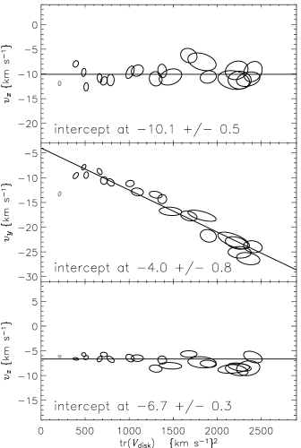
Figure 2: The mean velocity $\mathbf{v}_{\mathrm{disk}}$ as a function of total velocity variance $\mathrm{tr}(\mathbf{V}_{\mathrm{\!disk}})$ for the determination of the local standard of rest (LSR). In each panel, the ellipses indicate the one-sigma uncertainty regions (from bootstrap resampling—see text) of the measurements. The linear fit of $V$ vs. $S^{2}$ was performed with the projected Gaussian mixtures algorithm because it accounts correctly for the finite errors in both dimensions (see text). The point shown in grey was excluded from the fit because the stars in that subsample are very short-lived (see text). The reported uncertatinties on the intercepts are from 20 bootstrap resamplings of the ellipsoidal points shown.

Table 1 gives the 10 parameters, uncertainties, and uncertainty correlation matrix, for one of the subsamples. Figure 2 shows the mean $\mathbf{v}_{\mathrm{disk}}$ of the disk velocity distribution as a function of the trace $\mathrm{tr}(\mathbf{V}_{\mathrm{\!disk}})$ of its variance tensor $\mathbf{V}_{\mathrm{\!disk}}$. The mean velocity in the $\mathbf{\hat{y}}$ direction is a strong function of velocity dispersion; this linear dependence justifies the standard methodology for determination of the local standard of rest (LSR).

Operationally, the LSR is defined to be the mean velocity for a hypothetical population of stars with zero velocity distribution, i.e., the extrapolation to $\mathrm{tr}(\mathbf{V}_{\mathrm{\!disk}})=0$ of the trend shown in Figure 2. The points in Figure 2 have significant uncertainties in both dimensions, so fitting a line responsibly is not trivial. For this purpose we use again the projected mixtures of Gaussians procedure described above, but now there are 19 2-dimensional data points $\mathbf{w}_{i}$, the $\mathbf{w}_{i}$ and $\mathbf{v}_{i}$ are the same (i.e., the $\mathbf{R}_{i}$ are the identity matrices), and we only fit a single Gaussian ellipsoid. The straight line shown in the $\mathbf{\hat{y}}^{\scriptscriptstyle\top}\,\mathbf{v}_{\mathrm{disk}}$ ($v_{y}$) panel of Figure 2 is the principal eigenvector of the best-fit Gaussian. The $\mathbf{\hat{x}}^{\scriptscriptstyle\top}\,\mathbf{v}_{\mathrm{disk}}$ and $\mathbf{\hat{z}}^{\scriptscriptstyle\top}\,\mathbf{v}_{\mathrm{disk}}$ ($v_{x}$ and $v_{z}$) panels show simply weighted averages. The errors in the fit are computed by bootstrap resampling the 19 samples themselves.

The fits shown in Figure 2 provide an intercept corresponding to the estimated velocity relative to the Sun of a hypothetical population with vanishing velocity dispersion. The velocity of the Sun relative to this LSR is therefore

$$\mathbf{v}_{\odot}=-\mathbf{v}_{\mathrm{LSR}}$$ (10)

$$\mathbf{v}_{\odot}=[10.1\pm 0.5~{}\mathrm{km\,s^{-1}}]\,\mathbf{\hat{x}}+[4.0\pm 0.8~{}\mathrm{km\,s^{-1}}]\,\mathbf{\hat{y}}+[6.7\pm 0.2~{}\mathrm{km\,s^{-1}}]\,\mathbf{\hat{z}}\;\;\;.$$ (11)

Recall that rejection of halo stars was accomplished by fitting the velocity field with two Gaussians, one of which was fixed at the halo parameters given in equation (1). Re-fitting with the halo velocity dispersion increased to $150~{}\mathrm{km\,s^{-1}}$ changes the inferred LSR by much less than the magnitude of its uncertainty.

The vertex deviation is defined to be the angle between the $x$ axis and the projection onto the $x$–$y$ plane of the eigenvector corresponding to the largest eigenvalue of the velocity variance tensor $\mathbf{V}_{\mathrm{\!disk}}$. The vertex deviation is shown as a function of stellar color for the 20 subsamples in Figure 3.

4 Algorithm tests

To test the algorithm, 20 subsamples of artificial 3-dimensional stellar velocities $\mathbf{v}_{i}$ were generated with a mixtures of Gaussians random sample generator. The distribution was made with two Gaussians, one for the halo, with parameters as assumed above, and one for the disk, with mean $\mathbf{v}_{\mathrm{disk}}$ and variance tensor $\mathbf{V}_{\mathrm{\!disk}}$ different for each subsample. The artificial $\mathbf{v}_{i}$ were projected into artificial measurements $\mathbf{w}_{i}$ using the same $\mathbf{R}_{i}$ as in the real 20 subsamples, and errors were added, drawn from two-dimensional Gaussian ellipsoids with the same variances as the measurement uncertainty covariance tensors $\SS_{i}$. I.e., the artificial data were given all of the observational properties of the real data (modulo the assumptions of this study).

For subsamples with mean color $(B-V)<0.1~{}\mathrm{mag}$, the artificial variance tensor $\mathbf{V}_{\mathrm{\!disk}}$ was set to the measured value (shown in Figure 1) for the subsample with $(B-V)\approx 0.05~{}\mathrm{mag}$, and for subsamples with mean $(B-V)>0.6~{}\mathrm{mag}$, the artificial tensor $\mathbf{V}_{\mathrm{\!disk}}$ was set to the measured value for the subsample with $(B-V)\approx 0.67~{}\mathrm{mag}$. In between, i.e., for artificial subsamples with mean color $0.1<(B-V)<0.6~{}\mathrm{mag}$, the variance tensor was made to vary quadratically with color, so as to approximate the appearance of the true observations (and span the range of observed variance tensors. The artificial mean $\mathbf{v}_{\mathrm{disk}}$ was set to a linear function of the trace $\mathrm{tr}(\mathbf{V}_{\mathrm{\!disk}})$ of the variance.

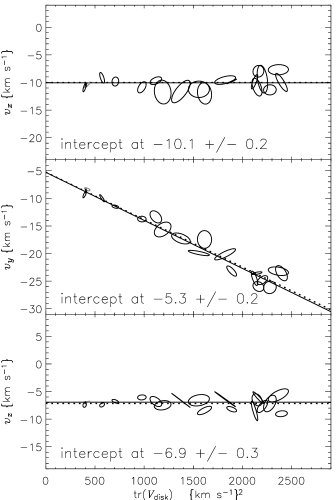
Figure 5: Same as Figure 2, but for the artificial data (see text). In each panel there is a dotted line indicating the input values used to make the artificial data.

Exactly the same fitting code and bootstrap analysis was applied to the artificial data as was applied to the real data. The results are shown in Figures 4 and 5, along with the input values used to make the artificial data. The best-fit parameters are, except for a couple of samples, within one standard deviation of the input paramters. More importantly for present purposes, the LSR is very well determined; the algorithm returns the correct LSR velocity to well within one standard deviation. We conclude that the algorithm is not significantly biased.

5 Generalized multi-Gaussian disk

Perhaps the biggest limitation of LSR measurements like this one is that the disk velocity distribution function is far from Gaussian; it is not even unimodal (Dehnen, 1998; Skuljan et al., 1999; Chereul et al., 1998); one of the primary goals of our future work is to explore the complexities of disk star velocities. As a baby step towards checking the influence of disk velocity non-Gaussianity on the LSR determination, the model was generalized to allow for not just one Gaussian ellipsoid to fit the each color subsample’s disk velocity distribution function but $K_{\mathrm{disk}}>1$ Gaussians, all constrained to have the same mean. Models with $K_{\mathrm{disk}}>1$ have the freedom to have larger “tails” to the velocity distribution, and for those tails to be rotated or twisted in velocity space relative to the core of the velocity distribution.

The generalized model is optimized by an algorithm constructed exactly parallel to that of the $K_{\mathrm{disk}}=1$ model, but now there are $4+6\,K_{\mathrm{disk}}$ free parameters for each subsample.

Increasing $K_{\mathrm{disk}}$ increases the goodness-of-fit (of course), but at very large $K_{\mathrm{disk}}$, the data will be “overfit”. To determine the optimal value of $K_{\mathrm{disk}}$ for each of the 20 stellar subsamples (the optimal $K_{\mathrm{disk}}$ will, in general, be different for different subsamples, of course), a “jackknife likelihood” was computed: For each of 5 iterations, a randomly selected 10 percent of each subsample was removed and put aside as a “test set.” Fitting (i.e., parameter determination by maximum likelihood) was performed on the remaining 90 percent, and the likelihood of the test set was tested within the context of the best-fit model. The logarithms of the jackknife likelihoods for the five iterations were averaged and the $K_{\mathrm{disk}}$ with the best jackknife likelihood was chosen for each subsample.

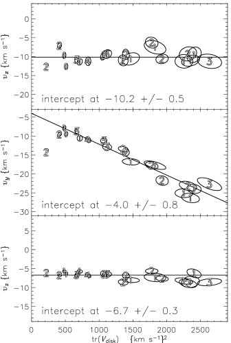
Figure 6: Same as Figure 2, but for the generalized model in which the disk velocity distribution is fit with a mixture of $K_{\mathrm{disk}}$ Gaussian ellipsoids with common mean. Each datapoint shows the result for that subsample for the optimal jackknife value of $K_{\mathrm{disk}}$ (see text), and is labeled by that value of $K_{\mathrm{disk}}$.

Figure 6 shows the LSR determination when the generalized model is used and each sample is fit with the optimal jackknife likelihood value of $K_{\mathrm{disk}}$. The velocity of the Sun relative to the LSR we find when using the optimal $K_{\mathrm{disk}}$ values is

$$\mathbf{v}_{\odot}=[10.2\pm 0.5~{}\mathrm{km\,s^{-1}}]\,\mathbf{\hat{x}}+[4.0\pm 0.8~{}\mathrm{km\,s^{-1}}]\,\mathbf{\hat{y}}+[6.7\pm 0.2~{}\mathrm{km\,s^{-1}}]\,\mathbf{\hat{z}}\;\;\;.$$ (12)

This is extremely similar to (much closer than 1 standard deviation away from) that found using $K_{\mathrm{disk}}=1$ (Figure 2). This suggests that that the assumption of Gaussianity is not strongly affecting the results.

6 Discussion

In the above, we developed and used a novel algorithm to infer the three-dimensional velocity distribution from a kinematically unbiased sample of Hipparcos stars.

The local velocity dispersion is a strong function of stellar color, and the mean velocity of a color-selected stellar population is a linear function of its velocity variance; this confirms previous results (e.g., Dehnen & Binney, 1998). The extrapolation of this relation to zero velocity dispersion provides an estimate of the local standard of rest (LSR), which is found to be

$$\mathbf{v}_{\odot}=[10.1\pm 0.5~{}\mathrm{km\,s^{-1}}]\,\mathbf{\hat{x}}+[4.0\pm 0.8~{}\mathrm{km\,s^{-1}}]\,\mathbf{\hat{y}}+[6.7\pm 0.2~{}\mathrm{km\,s^{-1}}]\,\mathbf{\hat{z}}\;\;\;,$$ (13)

where $\mathbf{\hat{x}}$, $\mathbf{\hat{y}}$, and $\mathbf{\hat{z}}$ are unit vectors pointing in the directions of the standard Galactic velocity components $U$, $V$, and $W$. This result is similar to previouw LSR determinations; we compare this result to one previous study below. Our answer did not change much when we relaxed the assumption that the disk star velocity distributions can be modeled as Gaussians.

We also showed that it is possible to robustly and reliably solve a missing data problem in astrophysics: the reconstruction of aspects of the three-dimensional velocity distribution function from individual velocity measurements every one of which is missing data in the radial direction.

Dehnen & Binney (1998), using the same subsample of the same data set, find a somewhat different Solar velocity relative to the LSR; they find

$$\mathbf{v}_{\odot}=[10.00\pm 0.36~{}\mathrm{km\,s^{-1}}]\,\mathbf{\hat{x}}+[5.25\pm 0.62~{}\mathrm{km\,s^{-1}}]\,\mathbf{\hat{y}}+[7.17\pm 0.38~{}\mathrm{km\,s^{-1}}]\,\mathbf{\hat{z}}\;\;\;,$$ (14)

They also find a lower mean velocity variance for the long-lived disk stars. These two differences are probably related, since the LSR is determined by fitting the relationship between velocity and velocity variance. Although the studies agree to within about one standard deviation, better agreement might be expected since both studies are using identical data subsets of the same data set. Both studies have made the incorrect assumption that the stellar velocity distribution is Gaussian; Dehnen & Binney (1998) did so in subtracting a measurement uncertainty variance from the measured velocity variance. The method presented here has been shown (using the generalized multi-Gaussian disk model) to be insensitive to the Gaussianity of the velocity distribution. The incorrect assumption of Gaussianity, entering differently in the Dehnen & Binney (1998) investigation, may account for the difference between the results. Because our method involves the optimization of a well-defined objective, because we have tested our method successfully with artificial data, and because we have been able to relax the Gaussian assumption, we prefer our result. Certainly the differences show that stellar velocity studies have become precise enough that algorithms matter. However, it must be emphasized that the true velocity distribution is far from a unimodal Gaussian (Dehnen, 1998; Skuljan et al., 1999; Chereul et al., 1998), so it is not clear that it is possible to make a “correct” LSR determination at all.

Appendix A Fitting Mixtures with Incomplete Data using the EM algorithm

The EM algorithm (Dempster et al., 1977) can be used to optimize the likelihood function of a probabilistic model involving incomplete observation data (hidden variables). Starting from user-supplied starting parameters, its iterations generate a sequence of parameters which monotonically increase the likelihood of a fixed data set under the model; thus it finds locally maximum likelihood parameters.

EM proceeds by optimizing, at each point in parameter space, a new function which is a strict lower bound on the data likelihood. This new functions depends on the original model parameters as well as on some extra auxiliary quantities introduced by EM. The EM algorithm iteratively increases the lower bound by coordinate ascent: first (the “M step”) the original model parameters are optimized (holding the auxiliary quantities fixed) and then (the “E step”) the auxiliary quantities are optimized (with the parameters fixed). After the optimization of the auxiliary quantities, the new function actually becomes equal to the true model likelihood (the bound becomes tight); thus at each iteration this true likelihood is nondecreasing. The M and E steps are iterated to convergence, which, here as usually, is identified by extremely small incremental improvement in the logarithm of the likelihood per iteration.

In particular, for any auxiliary distribution $q(\mathbf{v},j|\mathbf{w})$ we can lower bound the model likelihood $\ln p(\mathbf{w})$ by a functional $F(q)$. (In what follows, we slightly abuse notation by using $j$ both as an index and as a random variable representing the identity of the mixture component responsible for generating a particular data point.)

$$\displaystyle\ln p(\mathbf{w}|\theta) = \ln\sum_{j}\int_{\mathbf{v}}p(\mathbf{w},\mathbf{v},j|\theta)\,\mathrm{d}\mathbf{v}$$

$$\geq \sum_{j}\int_{\mathbf{v}}q\,\ln\frac{p(\mathbf{w},\mathbf{v},j|\theta)}{q}\,\mathrm{d}\mathbf{v}=F(\mathbf{w}|q,\theta)$$

$$\geq F(\mathbf{w}|q,\theta)=\sum_{j}\int_{\mathbf{v}}q(\mathbf{v},j|\mathbf{w})\,\left[\ln p(\mathbf{w},\mathbf{v},j|\theta)-\ln q(\mathbf{v},j|\mathbf{w})\right]\,\mathrm{d}\mathbf{v}$$

$$\ln p(\mathbf{w}|\theta) \geq F(\mathbf{w}|q,\theta)=\left\langle\ln p(\mathbf{w},\mathbf{v},j|\theta)\right\rangle_{q}+{\cal H}(q)\;\;\;,$$ (A1)

where $\theta$ represents the set of model parameters, and ${\cal H}$ is the entropy of the distribution $q$.

Our strategy is now coordinate maximization of $F$.

In the E step we maximize $F$ with respect to the auxiliary distribution $q$. It is easy to show (for example by checking that it saturates the bound on $F$) that the maximizing distribution $q$ is the conditional distribution of $\mathbf{v}$ and $j$ given the observations $\mathbf{w}$ and the current parameters:

$$\mbox{{E~{}step:}}\;\;\;q(\mathbf{v},j)\leftarrow\mathrm{argmax}_{q}F(\mathbf{w}|q,\theta)=p(\mathbf{v},j|\mathbf{w},\theta)\;\;\;.$$ (A2)

In the M step we maximize $F$ with respect to the parameters $\theta$. This maximization reduces to maximization of the expected complete log likelihood under the current variational distribution (since the entropy of $q$ does not depend on $\theta$):

$$\mbox{{M~{}step:}}\;\;\;\theta\leftarrow\mathrm{argmax}_{\theta}F(\mathbf{w}|q,\theta)=\mathrm{argmax}_{\theta}\sum_{j}\int_{\mathbf{v}}q(\mathbf{v},j)\,\ln p(\mathbf{w},\mathbf{v},j|\theta)\,\mathrm{d}\mathbf{v}\;\;\;.$$ (A3)

A.1 EM algorithm for projected mixtures

For the projected mixtures model the parameters consist of the mixture component amplitudes $\alpha_{j}$, means $\mathbf{m}_{j}$, and variances $\mathbf{V}_{\!j}$. The auxiliaries are posterior distributions for each star $i$: $q(j|\mathbf{w}_{i})$ over mixture components and $q(\mathbf{v}|j,\mathbf{w}_{i})$ over the true velocity (given the observed projected velocity, assuming it came from a specific component). In the terninology of this Appendix, the parameters of the probability distribution for the true 3-space velocity $\mathbf{v}$ of each star, including especially the probabilities that the star was drawn from each of the gaussian velocity components $j$, are the “auxiliary quantities,” and the parameters (amplitudes, means, and velocity variance tensors) of the velocity components $j$ are the “model parameters.”

First we consider the E step, in which the auxiliary distributions $q(\mathbf{v},j|\mathbf{w}_{i},\theta)$ are optimized. In the case of projected mixtures, the posterior over $\mathbf{v},j$ given $\mathbf{w}$ and the model parameters $\theta$ is itself a conditional mixture of Gaussians:

$$\displaystyle\mbox{{E~{}step:}}\;\;\;p(\mathbf{v},j|\mathbf{w}) = p(j|\mathbf{w})\,p(\mathbf{v}|j,\mathbf{w})$$

$$p(j|\mathbf{w}_{i}) = \frac{\alpha_{j}\,{\cal N}(\mathbf{w}|\mathbf{R}\,\mathbf{m}_{j},\mathbf{T}_{j})}{\displaystyle\sum_{k}\alpha_{k}\,{\cal N}(\mathbf{w}|\mathbf{R}\,\mathbf{m}_{k},\mathbf{T}_{k})}$$

$$p(\mathbf{v}|\mathbf{w}_{i},j) = {\cal N}(\mathbf{v}|\mathbf{b}_{ij},\mathbf{B}_{ij})$$

$$\mathbf{b}_{ij} = \mathbf{m}_{j}+\mathbf{V}_{\!j}\,\mathbf{R}_{i}^{\scriptscriptstyle\top}\,\mathbf{T}_{ij}^{-1}\,(\mathbf{w}-\mathbf{R}_{i}\,\mathbf{m}_{j})$$

$$\mathbf{B}_{ij} = \mathbf{V}_{\!j}-\mathbf{V}_{\!j}\,\mathbf{R}_{i}^{\scriptscriptstyle\top}\,\mathbf{T}_{ij}^{-1}\,\mathbf{R}_{i}\,\mathbf{V}_{\!j}^{\scriptscriptstyle\top}\;\;\;;$$ (A4)

Thus, the optimal choice for $q(\mathbf{v},j|\mathbf{w}_{i},\theta)$ is:

$$\displaystyle q(\mathbf{v},j|\mathbf{w}_{i}) = q(j|\mathbf{w}_{i})\,q(\mathbf{v}|j,\mathbf{w}_{i})$$

$$q(j|\mathbf{w}_{i}) = q_{ij}=p(j|\mathbf{w}_{i})$$

$$q(\mathbf{v}|\mathbf{w}_{i},j) = {\cal N}(\mathbf{v}|\mathbf{b}_{ij},\mathbf{B}_{ij})$$ (A5)

For the M step updates, we must explicitly write out the form of the functional $F$ and take its partial derivatives with respect to each set of model parameters:

$$\displaystyle F = \sum_{i}\left\langle\ln p(\mathbf{w}_{i}|\mathbf{v}_{i})+\ln p(\mathbf{v}_{i}|j)+\ln p(j)\right\rangle_{q_{i}}+{\cal H}(q_{i})$$ (A6)

$$= -\frac{1}{2}\sum_{i}\sum_{j}q_{ij}\left[\left\langle(\mathbf{w}_{i}-\mathbf{R}_{i}\mathbf{v})^{\scriptscriptstyle\top}\SS_{i}^{-1}(\mathbf{w}_{i}-\mathbf{R}_{i}\mathbf{v})(\mathbf{v}-\mathbf{m}_{j})^{\scriptscriptstyle\top}\mathbf{V}_{\!j}^{-1}(\mathbf{v}-\mathbf{m}_{j})\right\rangle_{q(\mathbf{v}|\mathbf{w}_{i},j)}\rule[-4.30554pt]{0.0pt}{12.91663pt}\right.$$

$$\quad\quad\quad\quad\quad\quad\left.\rule[-4.30554pt]{0.0pt}{12.91663pt}+\ln\det\SS_{i}+\ln\det\mathbf{V}_{\!j}+\log\alpha_{i}\right]$$

$$= -\frac{1}{2}\sum_{i}\sum_{j}q_{ij}\left[\mathbf{w}_{i}^{\scriptscriptstyle\top}\SS_{i}^{-1}\mathbf{w}_{i}+\mathbf{m}_{j}^{\scriptscriptstyle\top}\mathbf{V}_{\!j}^{-1}\mathbf{m}_{j}-2\mathbf{w}_{i}^{\scriptscriptstyle\top}\SS_{i}^{-1}\mathbf{R}_{i}\mathbf{b}_{ij}-2\mathbf{m}_{j}^{\scriptscriptstyle\top}\mathbf{V}_{\!j}^{-1}\mathbf{b}_{ij}\rule[-4.30554pt]{0.0pt}{12.91663pt}\right.$$

$$\quad\quad\quad\quad\quad\quad\left.\rule[-4.30554pt]{0.0pt}{12.91663pt}+\mathrm{Trace}\left[(\mathbf{R}_{i}^{\scriptscriptstyle\top}\SS_{i}^{-1}\mathbf{R}_{i}+\mathbf{V}_{\!j}^{-1})(\mathbf{b}_{ij}\mathbf{b}_{ij}^{\scriptscriptstyle\top}+\mathbf{B}_{ij})\right]\rule[-4.30554pt]{0.0pt}{12.91663pt}\right.$$

$$\quad\quad\quad\quad\quad\quad\left.\rule[-4.30554pt]{0.0pt}{12.91663pt}+\ln\det\SS_{i}+\ln\det\mathbf{V}_{\!j}+\log\alpha_{i}\right]$$

Deriving the E step and M step for the particular projected mixtures model given above leads to the following update equations:

$$\displaystyle\mbox{{M~{}step:}}\;\;\;\alpha_{j} \leftarrow \frac{1}{N}\,\sum_{i}q_{ij}$$

$$\mathbf{m}_{j} \leftarrow \frac{1}{q_{j}}\,\sum_{i}q_{ij}\,\mathbf{b}_{ij}$$

$$\mathbf{V}_{\!j} \leftarrow \frac{1}{q_{j}}\,\sum_{i}q_{ij}\left[(\mathbf{m}_{j}-\mathbf{b}_{ij})\,(\mathbf{m}_{j}-\mathbf{b}_{ij})^{\scriptscriptstyle\top}+\mathbf{B}_{ij}\right]$$

$$\mathbf{T}_{ij} \leftarrow \mathbf{R}_{i}\,\mathbf{V}_{\!j}\,\mathbf{R}_{i}^{\scriptscriptstyle\top}+\SS_{i}\;\;\;.$$ (A7)

Some care must be taken to implement these equations in a numerically stable way. In particular, care should be taken to avoid underflow when computing the ratio of a small probability over the sum of other small probabilities. Notice that we don’t have to explicitly enforce constraints on parameters, e.g., keeping covariances symmetric and positive definite, since this is taken care of by the updates. For example, the update equation for $\mathbf{V}_{\!j}$ is guaranteed by its form to produce a symmetric nonnegative definite matrix.

Figure 1: The best-fit parameters of the model as a function of stellar color for the 20 color-selected subsamples. The off-diagonal elements of the velocity variance tensor $\mathbf{V}_{\mathrm{\!disk}}$ have been scaled by square-roots of products of the diagonal elements.

Table 1: example parameter set for the subsample with $0.654<(B-V)<0.685$

parameter	value	units	correlation matrix of the (squared) uncertainties
$\mathbf{\hat{x}}^{\scriptscriptstyle\top}\,\mathbf{v}_{\mathrm{disk}}$	$-9.3\pm 1.9$	$\mathrm{km\,s^{-1}}$	$1.00$	$0.20$	$0.05$	$0.10$	$-0.14$	$0.38$	$-0.49$	$-0.30$	$0.16$	$-0.53$
$\mathbf{\hat{y}}^{\scriptscriptstyle\top}\,\mathbf{v}_{\mathrm{disk}}$	$-23.2\pm 1.3$	$\mathrm{km\,s^{-1}}$	$0.20$	$1.00$	$0.39$	$-0.23$	$-0.37$	$-0.08$	$0.12$	$0.18$	$-0.07$	$0.24$
$\mathbf{\hat{z}}^{\scriptscriptstyle\top}\,\mathbf{v}_{\mathrm{disk}}$	$-8.9\pm 1.1$	$\mathrm{km\,s^{-1}}$	$0.05$	$0.39$	$1.00$	$-0.42$	$-0.17$	$0.03$	$0.09$	$0.28$	$-0.30$	$-0.02$
$\mathbf{\hat{x}}^{\scriptscriptstyle\top}\,\mathbf{V}_{\mathrm{\!disk}}\,\mathbf{\hat{x}}$	$1329.\pm 95.$	$\mathrm{km^{2}\,s^{-2}}$	$0.10$	$-0.23$	$-0.42$	$1.00$	$0.37$	$-0.04$	$-0.10$	$-0.19$	$0.36$	$-0.24$
$\mathbf{\hat{y}}^{\scriptscriptstyle\top}\,\mathbf{V}_{\mathrm{\!disk}}\,\mathbf{\hat{y}}$	$474.\pm 58.$	$\mathrm{km^{2}\,s^{-2}}$	$-0.14$	$-0.37$	$-0.17$	$0.37$	$1.00$	$-0.30$	$0.21$	$0.07$	$0.53$	$-0.02$
$\mathbf{\hat{z}}^{\scriptscriptstyle\top}\,\mathbf{V}_{\mathrm{\!disk}}\,\mathbf{\hat{z}}$	$418.\pm 47.$	$\mathrm{km^{2}\,s^{-2}}$	$0.38$	$-0.08$	$0.03$	$-0.04$	$-0.30$	$1.00$	$0.04$	$0.02$	$-0.05$	$-0.47$
$\mathbf{\hat{x}}^{\scriptscriptstyle\top}\,\mathbf{V}_{\mathrm{\!disk}}\,\mathbf{\hat{y}}$	$95.\pm 46.$	$\mathrm{km^{2}\,s^{-2}}$	$-0.49$	$0.12$	$0.09$	$-0.10$	$0.21$	$0.04$	$1.00$	$0.27$	$0.00$	$0.15$
$\mathbf{\hat{x}}^{\scriptscriptstyle\top}\,\mathbf{V}_{\mathrm{\!disk}}\,\mathbf{\hat{z}}$	$11.\pm 56.$	$\mathrm{km^{2}\,s^{-2}}$	$-0.30$	$0.18$	$0.28$	$-0.19$	$0.07$	$0.02$	$0.27$	$1.00$	$-0.54$	$0.19$
$\mathbf{\hat{y}}^{\scriptscriptstyle\top}\,\mathbf{V}_{\mathrm{\!disk}}\,\mathbf{\hat{z}}$	$32.\pm 44.$	$\mathrm{km^{2}\,s^{-2}}$	$0.16$	$-0.07$	$-0.30$	$0.36$	$0.53$	$-0.05$	$0.00$	$-0.54$	$1.00$	$0.05$
$\alpha_{\mathrm{halo}}$	$0.0081\pm 0.0052$		$-0.53$	$0.24$	$-0.02$	$-0.24$	$-0.02$	$-0.47$	$0.15$	$0.19$	$0.05$	$1.00$

Figure 3: The vertex deviation (see text for definition) as a function of color.

Figure 4: Same as Figure 1, but for the artificial data (see text). The dotted lines indicate the input values used to make the artificial data.

References

- Bienaymé (1999) Bienaymé, O. 1999, A&A, 341, 86
- Binney et al. (2000) Binney, J., Dehnen, W., & Bertelli, G. 2000, MNRAS, 318, 658
- Chereul et al. (1998) Chereul, E., Crézé, M., & Bienaymé, O. 1998, A&A, 340, 384
- Chereul et al. (1999) Chereul, E., Crézé, M., & Bienaymé, O. 1999, A&AS, 135, 5
- Dehnen (1998) Dehnen, W. 1998, AJ, 115, 2384
- Dehnen (2000) Dehnen, W. 2000, AJ, 119, 800
- Dehnen & Binney (1998) Dehnen, W. & Binney, J. J. 1998, MNRAS, 298, 387
- Dempster et al. (1977) Dempster, A. P., Laird, N. M., & Rubin, D. B. 1977, Journal of the Royal Statistical Society series B, 39, 1
- ESA (1997) ESA. 1997, The Hipparcos Catalogue (ESA SP-1136)
- Fux (2001) Fux, R. 2001, A&A, 373, 511
- Lutz & Kelker (1973) Lutz, T. E. & Kelker, D. H. 1973, PASP, 85, 573
- Majewski et al. (2000) Majewski, S. R., Ostheimer, J. C., Kunkel, W. E., & Patterson, R. J. 2000, AJ, 120, 2550
- Quillen (2003) Quillen, A. C. 2003, AJ, 125, 785
- Sirko et al. (2004) Sirko, E., Goodman, J., Knapp, G. R., Brinkmann, J., Ivezić, Ž., Knerr, E. J., Schlegel, D., Schneider, D. P., & York, D. G. 2004, AJ, 127, 914
- Skrutskie et al. (1997) Skrutskie, M. F., Schneider, S. E., Stiening, R., Strom, S. E., Weinberg, M. D., Beichman, C., Chester, T., Cutri, R., Lonsdale, C., Elias, J., Elston, R., Capps, R., Carpenter, J., Huchra, J., Liebert, J., Monet, D., Price, S., & Seitzer, P. 1997, in ASSL Vol. 210: The Impact of Large Scale Near-IR Sky Surveys, 25–+
- Skuljan et al. (1999) Skuljan, J., Hearnshaw, J. B., & Cottrell, P. L. 1999, MNRAS, 308, 731
- York et al. (2000) York, D. et al. 2000, AJ, 120, 1579