On the excitation of PG1159-type pulsations

Stability properties are presented of dipole and quadrupole nonradial oscillation modes of model stars that experienced a late helium shell flash on their way to the white-dwarf cooling domain. The computed instability domains are compared with the observed hot variable central stars of planetary nebulae and the GW Vir pulsators.

1 Introduction

The family of pre-white dwarfs (PWDs) referred to as PG$1159$ stars is spectroscopically defined by the dominance of He II, C IV, and O VI (and sometimes N V) lines and a strong H deficiency. Surface mass abundances of about $33\%$ He, $50\%$ C and $17\%$ O are reported as typical. Currently, 32 stars are members of the PG$1159$ family, the effective temperatures range from about $170\,000$ to $80\,000$ K. Roughly half of the PG$1159$ stars are embedded in a planetary nebula.

Until recently, a hydrogen-deficient composition of the PG$1159$ kind could not be reconciled with stellar evolution scenarios. Only the introduction of appropriate overshooting and mixing procedures in modeling post-AGB stars undergoing a very late thermal pulse (VLTP) led to PWDs with H-deficient surface layers that are in agreement with PG$1159$ spectroscopy (Herwig, 2001, and references therein).

Ten of the PG$1159$ stars are pulsating variables (also baptized as GW Vir variables, after the variable-star designation of the prototype PG$1159$-035; we will use both names synonymously throughout the text). Four of the ten variable stars have high surface gravities ($\log g>7$) and low luminosities, i.e. they are essentially on the corresponding white-dwarf cooling track and have hence evolved around the “evolutionary knee” (cf. Fig. 1). The rest of the GW Vir stars has low $\log g$ (i.e. $\log g<7$), in four cases associated planetary nebulae are known. The observed periods range from about $5$ to some $17$ minutes on the high-$\log g$ branch and they can exceed one hour in the low-$\log g$ PG$1159$ variables. Based on these time-scales, the pulsations must be attributed to intermediate to high-order g modes.

The excitation physics of the PG$1159$-type oscillations is still a matter of debate; this, despite the relative simplicity of the microphysics in the destabilization region as compared with e.g. classical pulsating variables. Most of all, in the case of the PWD pulsations, the stability analyses are not discredited by the insufficiently understood rôle of convection which is usually present when the $\kappa$-mechanism is at work. Nonetheless, no general agreement exists regarding in particular the chemical composition in the driving zone (e.g. Starrfield et al., 1983; Saio, 1996; Bradley & Dziembowski, 1996; Gautschy, 1997; Cox, 2003; Quirion et al., 2004).

Saio (1996) and Gautschy (1997) studied qualitatively the influence of the new generation of opacity data, specifically of the OPAL opacities, on the excitation of GW Vir pulsations. Due to the lack of evolutionary models with realistic histories that led them through the thermally pulsing AGB phase, the authors performed their explorative computations on model stars that evolved off the helium main sequence. The evolutionary phases before the knee differed significantly from post-AGB tracks. The post-knee epochs though, converged surprisingly well towards the loci of full evolutionary computations. The PG$1159$-type instability regions deduced from the simplified models agreed decently well with observations. The computed period separations, however, differed sufficiently from the observed ones to arouse considerable criticism (O’Brien, 2000; Cox, 2003). However, it seems to have largely gone unrecognized that usually the excitation physics is much more robust than the asteroseismic signatures and that the studies of Saio (1996) and Gautschy (1997) served a useful purpose nonetheless.

In the following paper we return to the excitation physics of PG$1159$ stars. We set out to show that the Saio and Gautschy results are robust, as it has also been shown recently in an independent approach by Quirion et al. (2004). This time, we go beyond the use of simplified evolutionary models or the use of envelope models to describe GW Vir pulsations. Numerical stability analyses were performed on state-of-the-art model stars that evolved through a late helium shell flash after they evolved through the thermally pulsing AGB, starting originally from the main sequence. Hence, this paper closes the credibility gap left open by the earlier work. Section 2 introduces the stellar models and reiterates on the computational tools used for the stability analyses. Section 3 presents the results of the stability computations for dipole and quadrupole modes; in particular the instability domains are described. The results are discussed and compared with earlier work in Sect. 4; the conclusions in Sect. 5 point out further steps that need to be taken.

2 Models and Tools

Figure 1: Evolutionary track of the initially $2.7\mathrm{M}_{\odot}$ star passing through the AGB, a very late thermal pulse (VLTP), and entering the final cooling phase as a hydrogen-deficient white dwarf with $0.59\mathrm{M}_{\odot}$. Pulsation computations were performed at late epochs along the locus tracing the terminal departure from the red-giant domain.

The model stars on which stability analyses were performed were extracted from the computations described in Althaus et al. (2005); they followed an initially $2.7\mathrm{M}_{\odot}$ star with solar composition from the zero-age main sequence, through the AGB and a VLTP, to the final cooling sequence as a hydrogen-deficient white dwarf. Except for the final white-dwarf cooling phase, the admixture of heavy elements in the star’s envelope was assumed to be solar; the OPAL opacity tables that entered the computations are described in Althaus et al. (2005). The abundance evolution of $16$ chemical elements was included via a time-dependent numerical scheme that simultaneously treated nuclear evolution and mixing processes due to convection and overshooting. Such a treatment is particularly important during the short-lived phase of the VLTP and the born-again episode for which the assumption of instantaneous mixing is inadequate. In the course of the VLTP phase, most of the residual hydrogen envelope is engulfed by the deep helium-flash induced convection zone and is completely burned. The star is then forced to evolve rapidly back to the red-giant region and eventually into the domain of the central stars of planetary nebulae at high effective temperatures but this time as a hydrogen-deficient, quiescent helium-burning object. We note that the inclusion of overshooting below the helium-flash convection zone leads naturally to surface abundances in agreement with those observed in PG$1159$ stars (see Fig. 2). In particular, also the N abundance is compatible with the range of observed ones (of the order of 0.01 in mass) in pulsating PG$1159$ stars (e.g. Dreizler & Heber, 1998; Werner, 2001).

Four model-star sequences, with $0.53$, $0.55$, $0.59$, and $0.64\mathrm{M}_{\odot}$, were analyzed in this paper. The $0.59\mathrm{M}_{\odot}$ sequence derived directly from the evolution computations of Althaus et al. (2005). Figure 1 displays the evolutionary track of the model with $2.7\mathrm{M}_{\odot}$ on the zero-age main sequence and $0.59\mathrm{M}_{\odot}$ at the end on the white-dwarf cooling track. The stellar models with $0.53$, $0.55$, and $0.64\mathrm{M}_{\odot}$ were derived from the $0.59\mathrm{M}_{\odot}$ sequence by changing the stellar mass to the appropriate value shortly after the termination of the born-again red-giant phase of the VLTP (i.e. at $\log T_{\rm eff}\approx 4.2$). Upon restarting the evolution of the models with the abruptly changed mass, the efficiency of the helium-burning shell did not match the model structure. For all three stellar masses, the transition phase during which nuclear burning and the internal structure re-adapted lasted to about $\log T_{\rm eff}=5.1$ on the locus of the last descent from the red-giant domain.

Furthermore, the evolutionary phase along the white-dwarf cooling track (when $\log T_{\rm eff}<5.0$) included elemental diffusion which is important for the occurrence of a red edge of the pulsations as discussed in Sect. 3.2.

Figure 2: Representative spatial abundance profiles for selected nuclear species for a $0.59\mathrm{M}_{\odot}$ model at $\log T_{\rm eff}=5.15$ and $\log L/\mathrm{L}_{\odot}=2.377$. The outermost $10^{-5}M_{\ast}$ are not shown as the compositions do not change there anymore; this applies to the evolutionary phases prior to $\log T_{\rm eff}=5.0$ along the white dwarf cooling track. Overshoot episodes during core helium burning and the AGB evolution left clear signatures in the abundance profiles: the step at $-0.3$ and the mountain-like feature at around $-1$ of the abscissa.

The nonradial stability analyses of dipole and quadrupole g modes were performed with the Riccati integration method of the linear nonadiabatic oscillation equations as used in the PG$1159$ study of Gautschy (1997); the approach was described for example in Gautschy et al. (1996). Again, we retained the nuclear terms in the stability equations to detect potentially existent $\epsilon$-driven instabilities. Convective energy transport is not important in the envelopes of the PG$1159$ stars. Hence, the stability computations neglected convection effects completely. The Riccati method was described on various occasions in the past; nevertheless, elementary misjudgments continue to prevail (e.g. Cox, 2003) and it seems necessary to emphasize once more that the Riccati approach is a shooting method. The spatial resolution that can be achieved in the pulsation computations is not limited by the number of spatial gridpoints approximating the stellar background model. All that is required is that the stellar model must resolve all the relevant physical quantities sufficiently well. The physical quantities that must be accessible to the pulsation integration at arbitrary spatial coordinates are then interpolated in the stellar background via a monotonized cubic polynomial (Steffen, 1992). The limitation of the radial mode order that was computed in this project (and any other before) was inflicted by the computing time that had to be invested per mode rather than by any numerical spatial resolution issue.

In this project, the Brunt-Väisälä (BV) data had to be spatially smoothed. Very crisp composition steps in the stellar interior, be they imposed by elaborate treatments of convective boundaries or artificially produced by the finite-difference methodology, cause spikes in the BV frequency. Shooting methods are particularly sensitive to spikes in the coefficients of the differential equations as they usually entail very short integration steps to spatially resolve such rapid changes. Arguing that such discontinuities are somewhat smeared out in a real star, we smoothed the BV frequency numerically to iron out the spikes but maintaining at the same time its broader features. The simple algorithm that was invoked computed the BV frequency iteratively at any point in the star as the average over its nearest neighbors and consequently removed narrow spikes efficiently.

3 Results

Figure 3: The boundaries of the instability domains on the $\log T_{\rm eff}$ – period domain. The left panel shows the dipole modes, the right panel contains the results for the quadrupole modes. The loci traced out by the four model sequences are plotted with different line types. For the $0.59\mathrm{M}_{\odot}$ sequence, the results obtained on models with suppressed diffusion are shown in addition with a thin dot-dot-dashed line in the left panel. The boxes delineate the observational situation for dipole modes. Details are given in the text.

This section describes the numerical results obtained from the nonadiabatic eigenanalyses of $\ell=1$ and $2$ modes, performed on the four model-star sequences with $0.53,0.55,0.59$, and $0.64\mathrm{M}_{\odot}$.

Figure 3 displays the instability boundaries on the $\log T_{\rm eff}$ – period plane for $\ell=1$ (left panel) and $\ell=2$ modes (right panel). Eigenmodes with periods up to $1800$ s were considered. For the dipole modes, the observed domains which are occupied by GW Vir variables are overlaid for comparison. The observed dipole-mode period ranges were adopted from Tab. 1 of Nagel & Werner (2004); the horizontal sizes of the boxes reflect the canonical 10 % uncertainty in the spectroscopic $T_{\rm eff}$ determinations.

The $\log T_{\rm eff}$ – period diagram for dipole modes shows that the instability regions are separated into a low-$\log g$ (high luminosity) and a high-$\log g$ (low luminosity) domain for each mass. For all stellar masses considered, the tip of the evolutionary knee is pulsationally stable. The low-$\log g$ instability domains are roughly compatible with observed periods in variable planetary-nebulae nuclei (PNNV). One exception is the star Lo4 with its short periods. The Lo4 observations could possibly be reconciled by adopting $M_{\ast}<0.53\mathrm{M}_{\odot}$.

No red edge was encountered in the low-$\log g$ instability domains. Due to our restriction of the computations on the long-period side, we could not follow overstable modes to temperatures below $125\,000$ K on the high-luminosity branch of the evolutionary tracks. At these longest periods that were computed, we did see no signs yet of a decline of the strength of the instabilities.

The high-$\log g$ instability domains start at $\log T_{\rm eff}=5.12$ for the $0.53\mathrm{M}_{\odot}$ model and at successively lower $T_{\rm eff}$s for higher masses. If elemental diffusion was included, all instability domains showed a sharply defined red edge on the $\log T_{\rm eff}$ – period plane. The $0.59\mathrm{M}_{\odot}$ model sequence was evolved once with diffusion at $\log T_{\rm eff}<5.0$ and once without diffusion. The resulting instability boundaries are displayed as dot-dot-dashed lines in the left panel of Fig. 3. For $\log T_{\rm eff}>4.98$ both instability domains are indistinguishable. The diffusive models encounter a red edge at $\log T_{\rm eff}\approx 4.97$. The instability domain of the diffusion-free sequence (thin dot-dot-dashed line), on the other hand, continues to grow towards lower $T_{\rm eff}$s without a sign of a weakening at $\log T_{\rm eff}=4.70$, the location of the coolest model analyzed.

The position of the red edge is not realistic; its location depends on the epoch when diffusion is switched on during the evolution computations. All that is important here is that diffusion causes a red edge; this point is further elaborated on in Sect. 3.2.

The maximal period-widths of the high-$\log g$ instability domains range from $290$ to $480$ s with no clear mass dependence. On the other hand, the magnitude of the shortest and the longest overstable periods are a function of mass. The $0.53\mathrm{M}_{\odot}$ models have the longest-period overstable modes; the magnitude of the upper period boundary decrease with increasing mass. For the $0.64\mathrm{M}_{\odot}$ sequence, the longest overstable period is as short as $500$ s. On the other side, the shortest-period overstable modes have periods as low as $192$ s for the $0.64\mathrm{M}_{\odot}$ sequence. This is shorter than the shortest observed periods in any GW Vir star.

The most obvious problem is evidently the prototype of the class, PG$1159$-035 itself. PG$1159$-035 lies so close to the evolutionary knee of the model tracks that it falls mostly between the low- and high-$\log g$ $\ell=1$ instability domains. The observational box on the $\log T_{\rm eff}$ – period plane overlaps only marginally with the instability domains of the $0.53\mathrm{M}_{\odot}$ sequences. Such a low mass must be rejected, however, based on the computed period separations (see also Sect. 4).

The right-hand panel of Fig. 3 shows the boundaries of the instability domains traced out by the quadrupole g modes. For the two most massive sequences, the instability topology looks the same as for the dipole modes. The main difference is that considerably shorter-period modes are overstable. For the $0.55$ and $0.53\mathrm{M}_{\odot}$ sequences, the instability domains are uninterrupted, they extend around the knee from the low- to the high-$\log g$ domain. The effective temperatures of the red edges of the dipole and quadrupole instability domains coincide. The growth rates of the overstable $\ell=2$ modes reach comparable magnitudes as those of the $\ell=1$ modes.

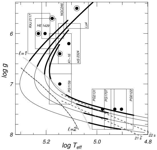
Figure 4: The GW Vir instability domains on the $\log T_{\rm eff}-\log g$ plane. The dots represent observed variable PG$1159$ stars. Encircled dots indicate the pulsators that are embedded in a planetary nebula. The boxes around the observational data mark the canonical uncertainties. The dotted line indicates the dipole-mode and the dash-dotted line the quadrupole blue edge. Along the evolutionary tracks, the epochs with overstable g modes are plotted with heavy lines. In the lower right of the figure, the two grey dashed lines mark the loci of constant period separation ($21$ s and $22$ s) as derived from the nonadiabatic stability computations.

For comparison with spectroscopically calibrated PG$1159$ stars, Fig. 4 plots the evolutionary tracks and the overstable regions on the $\log T_{\rm eff}$ – $\log g$ plane. Observed GW Vir stars and the associated error boxes are superimposed. PNNVs are indicated by encircled dots. The loci of the blue edges of $\ell=1$ and $2$ modes are given as dotted and dash-dotted lines, respectively. The evolutionary phases harboring overstable dipole g modes are marked with a heavier line on top of the evolutionary track. The general agreement between observations and models is reasonably good. Note again, the red edge position is not trustworthy. Important is, however, the existence of a red edge.

Figure 5: The loci of all model sequences in the PG$1159$ region of the HR plane. The heavy lines delineate the domains of unstable $\ell=1$ g modes. The blue edges for dipole and quadrupole modes, respectively, are indicated with broken lines. For $\log T_{\rm eff}>5.1$ at high luminosities of the $0.59\mathrm{M}_{\odot}$ models, no instability is indicated; most probably, however, overstable g-modes exist there. However, the computations were stopped because the shortest unstable periods exceeded $1800$ s.

Finally, Fig. 5 shows the evolutionary tracks of the model stars on the HR plane; thereon, the blue edges can be approximated by straight lines. The dipole-mode blue edge obeys the relation

$$\log L/\mathrm{L}_{\odot}=9.289\cdot\log T_{\rm eff}-45.186\,.$$ (1)

The dash-dotted line in Fig. 5, delineating the quadrupole-mode blue edge, is less steep than the $\ell=1$ blue edge and follows the relation

$$\log L/\mathrm{L}_{\odot}=9.0372\cdot\log T_{\rm eff}-44.158\,.$$ (2)

The above parameterizations of the blue edges imply a mass dependence of the GW Vir instability domains as it is already evident in Fig. 3. In Sect. 4, we return to the observation that the orientation of the blue edge on the HR plane differs from that of the classical instability strip, in particular the slope as the opposite sign.

3.1 The excitation mechanism

The g modes that are found overstable in our models are all driven by the $\kappa$-mechanism induced by the opacity bump peaking around $\log T=6.2$. Partial ionization of K-shell electrons in C and O cause the peak. As the matter of the stellar envelopes also contains heavy elements before the onset of diffusion, the high-temperature Z-bump enhances the opacity peak around $\log T=6$. Hence, the pulsation driving is the same as in all hitherto stability studies of PG$1159$ variables.

The abundance profile shown in Fig. 2 is representative of all models before the occurrence of diffusion-induced helium gradients in the outer envelopes (see Fig. 6). For the diffusion-less models, the abundances remain on the level as at the left border in Fig. 2 out to the photosphere. Note that in Fig. 2, the temperature reached already $1.6\cdot 10^{7}$ K at $\log(1-m/M_{\ast})=-5$. Hence, all model stars have at least $30.6\%$ of helium (in mass units) in the driving region. In particular, all oscillating PG$1159$ models with $\log T_{\rm eff}>5.0$ (on the white-dwarf cooling tracks) have no composition gradient between photosphere and the pulsations’ driving region. Therefore, the excitation physics remains the same as discussed by Saio (1996), Gautschy (1997), and more recently by Quirion et al. (2004).

3.2 The red edge

Figure 6: Top panel: Spatial variation of the He profile (Y) as a function of depth, measured in $\log T$, for four $0.55\mathrm{M}_{\odot}$ model stars as the red edge of the g-mode instability is approached. Bottom panel: Differential work, $w\equiv{\mathrm{d}}W/{\mathrm{d}}r$, of the $\ell=1,k=19$ mode for the same models. The eigenmode belonging to the thinnest line is pulsationally stable.

As mentioned before, all model sequences were evolved with switching on elemental diffusion after they passed $\log T_{\rm eff}=5.0$ on the white-dwarf cooling track. The choice of the epoch of the switch-on of diffusion was arbitrary. If diffusion alone, without competing counteracting physical transport processes, is considered, sedimentation is very effective. The top panel of Fig. 6 shows the helium profiles close to the g-mode driving region at several epochs of the $0.55\mathrm{M}_{\odot}$ model sequence. It took the star to evolve only from $\log T_{\rm eff}=5.0$ to $4.951$ for the superficial He abundance to rise from $0.306$ to $0.77$. The superficial flattening of the He profile is an artifact of the modeling procedure: the diffusion equations are solved only in the Henyey part of the stellar interior but not in the stellar envelopes that are computed in full equilibrium. Hence our results probably underestimate the diffusion effects.

As mentioned in Sect. 3, we computed also the stability properties of $0.59\mathrm{M}_{\odot}$ model stars devoid of diffusion. The corresponding stability analyses were hence performed on models with a constant He mass abundance of $0.306$ from the surface to the nuclear-active deep interior. Neglecting diffusion altogther for the whole evolutionary history, no damping of the g-mode pulsations was found along the white-dwarf cooling track.

On the other hand, if diffusion was accounted for, the g mode instabilities literally starved when the He abundance exceeded a critical level. The microphysics of elemental transport is such that the He that is going to float on top of the heavier elements starts to separate from these other elements at a temperature depth of about $10^{7}$ K. The steepest abundance gradients are found between $\log T=6.7$ and $6.3$, this region also dominates the damping and driving of the g-modes for the PG$1159$ variables. Hence, it is understandable that superseding the main driving elements of that region with “pulsationally inert” stellar material reduces the efficiency of the pulsational driving. Looking at the differential work curves in the lower panel of Fig. 6 shows indeed that the curves are essentially self-similar. The higher the helium abundance in the driving region the less efficient is the driving contribution to the pulsations. Finally, with Y$=0.77$ in the superficial layers in Fig. 6, the driving cannot compensate the damping anymore and the g modes turn stable. The critical level of helium above the driving region for the red edge varies between $0.77$ and about $0.82$ for the different masses of the model stars considered here.

The differential-work curves are very similar in form as the He abundance rises towards the surface; the compositional gradient does not distort the eigenfunctions (the spatial kinetic energy distribution is essentially unaffected by the diffusion process). Therefore, one can say that diffusion lets the pulsations “starve”. In the present computations, diffusion destroys the pulsations rather quickly after sedimentation is “switched on” at $T_{\rm eff}=100\,000$ K. The red edges of the different mass sequences were then encountered between $70\,800$ and $89\,100$ K. Approaching the red edge, the long-period modes died away earlier than the short-period ones. Therefore, close to the red edge, the mean period of the range of excited modes

4 Discussion

The splitting of the PG$1159$ pulsation domains (see Fig.  3) into two regions – a long-period, low-$\log g$ domain and a short-period, high-$\log g$ part – agrees with the results of Saio (1996) and Gautschy (1997). In the current computations, no continuous instability domain connecting low- and high-$\log g$ regions was found for dipole modes. In the two older studies just mentioned, the $0.56$ and $0.57\mathrm{M}_{\odot}$ sequences had continuous instability domains, however. The reason is connected with the different loci of the evolutionary tracks on the $T_{\rm eff}$ – $\log g$ plane, the present models reach higher $\log g$ values earlier in their evolution than in the old simplified ones of Saio and Gautschy.

Regarding the comparison with observations, there is essentially one problem case: PG$1159-0354$ itself. As mentioned before, on the $T_{\rm eff}$ – period plane, the observational box overlaps only slightly with the computed instability domains of the $0.53\mathrm{M}_{\odot}$ model sequence. Comparing the associated computed mean period-separation ($\overline{\Delta\Pi_{\ell=1}}=22.46$ s) with the observed one ($21.62$ s) makes it clear that the $0.53\mathrm{M}_{\odot}$ model is no acceptable solution. With regard to the period-separation, the best agreement was found with the $0.55\mathrm{M}_{\odot}$ model having $\overline{\Delta\Pi_{\ell=1}}=21.50$ s at $T_{\rm eff}=138\,000$ K. This, however, means that the $\ell=1$ blue edge is at least $6000$ K to cool there to be compatible with the observed situation. Our preferred mass for PG$1159-0354$ is closer to the spectroscopic calibration of Dreizler & Heber (1998) ($0.54\mathrm{M}_{\odot}$) than to the $0.59\mathrm{M}_{\odot}$ of Kawaler & Bradley (1994). The latter value is frequently regarded as kind of a canonical mass for PG$1159-0354$; it should, though, be kept in mind that the asteroseismic calibrations rely on fits to some evolutionary models with all their shortcomings and uncertainties.

According to the current models, regions of exclusively $\ell=2$ overstable modes were encountered for lower-mass (i.e. about $0.53<M_{\ast}<0.57\mathrm{M}_{\odot}$) PWDs when they pass along the low-luminosity side of the evolutionary knee.

As mentioned hitherto for DBVs (Gautschy & Althaus, 2002), also for the pulsating PG$1159$ models we found the shortest-period overstable modes to be quadrupole ones and the longest-period overstable modes to be dipole ones. Even if the latest RXJ$2117$ observations (Vauclair et al., 2002) do not clearly reveal quadrupole modes, the most likely $\ell=2$ candidates in the data are at the short-period boundary of the observed set. Also for PG$1159$ (Winget et al., 1991), the positively identified $\ell=2$ mode has a short period at $425$ s. However, one multiplet, the one associated with longest-period mode, is possibly due to an $\ell=2$ mode; if true, this would clearly contradict our computations. Another potential problem case is PG$0122$; its $465$ s mode – the third-longest period mode reported in O’Brien et al. (1996) – is suggested to be a quadrupole mode. The identification was not without debate, however.

With regard to mode excitation, we saw that neither the use of overly simplified full stellar models nor the use of envelope models only are the reason for overstable g modes in envelopes with helium mass abundances of about 0.3. Additionally, we have now three different numerical methods (finite-difference relaxation, finite-element solver, and a nonlinear shooting method) that agree on the g-mode excitation. The disagreeing results (e.g. Starrfield et al., 1983; Bradley & Dziembowski, 1996; Cox, 2003) were obtained with finite-difference relaxation methods which resemble the method of Saio (1996). We hypothesize therefore that the origin of the disagreement is linked to particularities of the computational realizations. We found the previously proclaimed “helium poisoning” to become effective only at higher mass abundances such as they are encountered when elemental diffusion was at work. If the relative mass abundance of helium exceeded about $0.77$, the g modes were found to “starve” so that a red edge occurred.

With respect to pulsational driving, the only qualitative difference to the results of Saio (1996) and Gautschy (1997) is the absence in the current model stars of $\epsilon$-driven instabilities with periods of around $100$ s.

How can the bimodal period distribution on the $T_{\rm eff}$ – period plane (cf. Fig. 3) be understood? At a chosen $T_{\rm eff}$, the periods differ by at least a factor of three, whereas the luminosities differ by factor of $15$ or more. In contrast to the expectations, the short periods are excited at low and long periods at high luminosities. To understand this, we resort to the classical time-scale argument (e.g. in Cox & Giuli, 1968)

$$\int_{\Delta M}\!\!\!c_{V}T\,{\mathrm{d}}m/L_{\ast}={\cal O}(\Pi/2\pi)\,.$$ (3)

The integral extends over the mass of the envelope, $\Delta M$, overlying driving region of the pulsations. Relation (3) defines the pulsation period, $\Pi$, for which the thermo-mechanical coupling in the stellar material is optimal for pulsational driving. We compared two $0.59\mathrm{M}_{\odot}$ models at $\log T_{\rm eff}=5.06$, one at high and the other at low luminosity. For both models, we evaluate the left-hand side in eq. (3). We approximate the integral, as usual, by adopting the values at the driving region for the quantities $c_{V}$ and $T$ (indicated by a tilde) and write it hence as $\tilde{c_{V}}\,\tilde{T}\,\Delta M$. Based on the full stability computations, we assumed the driving to occur at around $\log\tilde{T}=6.3$ in all cases. Therefore, we compute the ratios of $\tilde{c_{V}},\Delta M$, and $L_{\ast}$; all three quantities are considerably larger than unity as the evolution proceeds past the knee (always measured at the same $T_{\rm eff}$). It turns out that the product in the numerator of Eq. (3) over-compensates the change in $L_{\ast}$ in the denominator. Therefore, the high-luminosity phase of evolution prefers longer periods for pulsation than the low-luminosity one. The overcompensation is mainly due to the considerable decrease of the envelope mass, overlying the driving region, as the stars evolve towards to white-dwarf cooling track. At $\log T_{\rm eff}=5.06$ for example, $\Delta M$ at high $L_{\ast}$ is 630 times larger than at low $L_{\ast}$. The influence of this number is further enhanced by the fact that radiation pressure constitutes a considerable fraction of the total pressure, $P$, in the high-luminosity stage. Since $c_{V}\propto 1/\beta^{2}$, with $\beta=1-P_{\mathrm{rad}}/P$, $c_{V}$ can rise considerably when radiation pressure gains importance. Again, for the models at $\log T_{\rm eff}=5.06$ we found $\tilde{\beta}\approx 0.4$ at the high luminosity and $\tilde{\beta}\approx 0.9$ at the low-luminosity epoch.

To understand the slope/orientation of the blue edge in the post-knee domain in the HR diagram, we follow the reasoning of Cox & Hansen (1979). We approximate eq. (3) the same way as to understand the period bimodality. We approximate the hydrostatic equilibrium as

$$\frac{4\pi\tilde{P}R^{4}}{GM}\approx\Delta M\,.$$

The Stefan-Boltzmann relation allows to rewrite eq. (3) as

$$\frac{\tilde{c_{V}}\tilde{T}\tilde{P}L}{\Pi\,T_{\rm eff}^{8}\,M}\approx\text{const.}$$

The envelope $P-T$ structure of PWDs is decently approximated by a radiative-zero one using a Kramers-type opacity. Eliminate $\tilde{P}$ in the last equation with the chosen $P-T$ relation to get

$$\frac{\tilde{c_{V}}\tilde{T}^{5.25}}{\Pi\,T_{\rm eff}^{8}}\cdot\sqrt{\frac{L}{M}}\approx\text{const.}$$ (4)

For the period $\Pi$, we adopt the relation $\Pi\propto T_{m}^{-\frac{1}{2}}R$ from Winget et al. (1983). Using a very simple white-dwarf model from Kippenhahn & Weigert (1994) (their section 35.3): $T_{m}\propto\left({L}/{M}\right)^{{2}/{7}}$ to estimate the maximum temperature, $T_{m}$, leads to

$$\Pi\propto R\,\left(\frac{L}{M}\right)^{-\frac{1}{7}}\,.$$

Eliminating $R$ again via Stefan-Boltzmann’s law gives

$$\frac{\tilde{c_{V}}\tilde{T}^{5.25}}{T_{\rm eff}^{6}}\cdot\frac{L^{\frac{1}{7}}}{M^{\frac{9}{14}}}\approx\text{const.}$$ (5)

Assume the temperature at the top of the driving region, $\tilde{T}$, to remain constant within the instability domain of the PG$1159$ variables and neglect the mass dependence of the derived relation, as the range of stellar masses assigned to PG$1159$ variables is small. From fits to the evolutionary computations we derive ${\mathrm{d}}\ln\tilde{c_{V}}/{\mathrm{d}}\ln L|_{T_{\rm eff}}\approx 0.5$ and we neglect any additional $T_{\rm eff}$ dependence. All things considered, we finally arrive at:

$$\frac{{\mathrm{d}}\ln L}{{\mathrm{d}}\ln T_{\rm eff}}=\frac{28}{3}\approx 9.3\,.$$ (6)

According to eq. (1), the slope of the blue edge as obtained from the fit to the full nonadiabatic computations is $9.3$ for $\ell=1$ and $9.0$ for $\ell=2$. Regarding the simplicity of the model and the coarseness of the approximations, the result is astonishing. We attribute the dominant contribution to the slope of the blue edge to the term ${\mathrm{d}}\ln c_{V}/{\mathrm{d}}\ln L$. Hence, it is the growing importance of radiation pressure as the luminosity increases in the PG$1159$ envelopes that tilts the blue edge to the left on the HR- and the $\log T_{\rm eff}-\log g$ diagrams.

We found elemental diffusion to quench g-mode instability on the high-$\log g$ branch of evolution when the helium abundance exceeds a critical level in the driving region. A helium mass abundance of about $0.77$ was found to be sufficient for the overstable g modes to starve. Hence, as conjectured by Dreizler & Heber (1998), a depletion of C and O, which can be regarded complementarily as an enhancement of He, due to sedimentation in the driving region enforces a red edge.

Diffusion is a very efficient process to turn PG$1159$ stars into DO stars. If only diffusion – without counteracting processes – is included in stellar modeling, DO stars would show up at too high effective temperatures to be compatible with observations. In the current modeling, diffusion was switched on ad hoc at $100\,000$ K on the white-dwarf cooling track. Therefore, the location of the red edge of the PG$1159$ variables in the various diagrams shown in this paper is not trustworthy.

The quantitative non-equilibrium computations of Unglaub & Bues (2000) to model the counteracting processes of diffusion and mass loss suggest that a unique red edge for the PG$1159$ variables as a class cannot be expected. As compositions and rotational velocities (which tend to homogenize composition gradients) vary from star to star, also the epoch (and hence the corresponding $T_{\rm eff},L$, or $g$) will vary when the critical contamination of the driving region is reached. Therefore, it is not inconceivable that close to the red edge of the PG$1159$ variables, these are intermixed with stable DO stars and even with non-pulsating PG$1159$ stars. The closer one gets to the red edge, the shorter should the mean period of the excited modes be; this occurs since, according to our computations, the long-period modes starve earlier than the short-period ones.

The position of the theoretical instability domains is only part of the game to understand the GW Vir pulsators. Pertinent information is obtained from period-spacing data. We used the results from $\ell=1$ computations to compare them with the observed period separations for three stars. In the case of RXJ$2117+3412$, only tracks of $0.64$ and $0.59\mathrm{M}_{\odot}$ models pass on the $\log T_{\rm eff}-\log g$ plane within the observational error box. Inspecting the period separations revealed that the 0.64 models have too small a mean period separation. Even the $0.59\mathrm{M}_{\odot}$ objects with the arithmetic-mean period separation $\overline{\Delta\Pi_{\ell=1}}\approx 20.0$ s were below the mean observed separation of $21.62$ s (Vauclair et al., 2002). Hence, only a mass below $0.59\mathrm{M}_{\odot}$ can fit the observation. However, the corresponding current evolutionary tracks pass outside the error box. PG$1159-035$’s observed $\overline{\Delta\Pi_{\ell=1}}=21.62$ s period spacing (Winget et al., 1991) is best reproduced with our $0.55\mathrm{M}_{\odot}$ models. As mentioned before, the problem with the $0.55\mathrm{M}_{\odot}$ model stars is that none of the involved dipole modes is pulsationally overstable in the vicinity of the position of PG$1159-035$ on the $\log T_{\rm eff}-\log g$ plane. Again, evolutionary models that arrive at the lower side of the knee with higher luminosity than what we get currently might resolve the dilemma. Finally in PG$2131+066$, $\overline{\Delta\Pi_{\ell=1}}=21.65$ s is observed (Kawaler et al., 1995). From our current modeling, we conclude that the best fitting stellar mass lies between $0.55$ and $0.59\mathrm{M}_{\odot}$; the observed pulsation modes fall then well within the computed range of overstable dipole g modes (cf. Fig. 3).

Figure 4 has inscribed lines of constant period separations. The loci of $21$ s and $22$ s, interpolated from the nonadiabatic computations, are shown. Note that the observed period separations for RXJ$2117$, PG$1159-035$, PG$2131$, and (according to O’Brien, 2000) PG$0122$ all lie between $21$ and $22$ s. If PG$1707+427$’s period separation of $18.37$ s (Fontaine et al., 1991) holds then the apparent confinement to $21-22$ s of the other four GW Vir variables is an observational bias. However, in case the period separations of GW Vir stars are indeed narrowly confined, then they populate only a fraction of the instability region as computed by linear theory. It appears worthwhile to point out that the loci of constant period separation depend also on the trapping amplitude of the modes. Our mean period separations were computed as simple arithmetic means over many successive radial orders. The larger the trapping amplitudes are, i.e. the sharper the composition gradients in the stellar interior, the bigger the difference between $\overline{\Delta\Pi}$ and the asymptotic value. If mass-dependent diffusion efficiencies are capable to increase the distance between the, say $21$ and $22$ s, period-separation lines in Fig. 4 remains to be seen. On the observational side, the number of asteroseismically studied PG$1159$ is so low, that every additional well-resolved oscillation-frequency spectrum that becomes available makes an important contribution to solve this conundrum.

In addition to the period-separation information, we can also compute the lengths of the trapping cycles. The two comparisons with observations that are currently possible revealed the modeled trapping-cycle lengths to be always shorter than the observed ones: RXJ$2117+3412$, $83.9$ s observed and $56-60$ s computed. For PG$1159-035$: $80.5$ s observed and $52.6-68.4$ s computed. Based on mode-trapping theory as developed in Brassard et al. (1992), the current model stars have seemingly too thick helium layers to be compatible with observations. As there is ample evidence for mass loss before and during the PG$1159$ episodes of evolution (Werner, 2001), we are positive that the mass of the helium-rich model envelopes can be sufficiently reduced via a hot stellar wind to improve the agreement with observations.

5 Conclusions

The excitation physics as scraped out from simplified model stars by Saio (1996) and Gautschy (1997) is corroborated using now complex stellar-evolution models that went through a very late thermal flash. In particular, we found again that modes can be excited with considerable He abundance in the driving region, supporting the view that abundance gradients between the spectroscopically accessible stellar surface and the driving region of g modes do not have to be invoked to explain PG$1159$-type oscillations (e.g. Bradley & Dziembowski, 1996).

A blue edge was encountered for dipole and quadrupole modes; its slope is a manifestation of a mass dependence of the pulsational instability of PG$1159$ stars. On the high-luminosity branch of the evolutionary track, the hottest variables are the most massive ones. The situation reverses on the low-luminosity branch (below the evolutionary knee), where the bluest variables are the least massive ones.

Model-star sequences including diffusion led to a red edge of the PG$1159$ instability domain. Much in agreement with the predictions of Dreizler & Heber (1998), the oscillations of the PG$1159$ stars starve once the He abundance in the driving region exceeds a critical magnitude. It is therefore likely that the red edge is close to the transition from PG$1159$ to hot DO- or possibly DA-type white dwarfs. It is furthermore conceivable that the red edge of the GW Vir stars is not sharply defined but rather frayed. The counteracting effects of rotation, stellar wind, radiative levitation and gravitational settling determine for each star individually when the g-mode pulsations die out. A significant step ahead would be parameter studies of the competition of mass-loss and/or diffusion on the efficiency of pulsational driving. Currently, diffusion is still switched on ad-hoc.

In contrast to the models of Saio (1996) and Gautschy (1997), the stability analyses of the current stellar model sequences did not reveal any overstable $\epsilon$-mechanism driven g modes at short periods.

We gathered some evidence, when comparing the theoretical with the observed period-separation data, that the current evolutionary tracks evolve at too low luminosity on the HR diagram and hence on the $\log T_{\rm eff}-\log g$ plane. Furthermore, based on the magnitudes of the trapping-cycle lengths, the helium-rich envelopes of the current PG$1159$ models seem to be too massive to agree with observations. It appears therefore worthwhile to look again into the microphysics and the numerics of evolutionary computations to try to resolve the persisting discrepancies.