Weak Gravitational Flexion

Abstract

Flexion is the significant third-order weak gravitational lensing effect responsible for the weakly skewed and arc-like appearance of lensed galaxies. Here we demonstrate how flexion measurements can be used to measure galaxy halo density profiles and large-scale structure on non-linear scales, via galaxy-galaxy lensing, dark matter mapping and cosmic flexion correlation functions. We describe the origin of gravitational flexion, and discuss its four components, two of which are first described here. We also introduce an efficient complex formalism for all orders of lensing distortion. We proceed to examine the flexion predictions for galaxy-galaxy lensing, examining isothermal sphere and Navarro, Frenk & White (NFW) profiles and both circularly symmetric and elliptical cases. We show that in combination with shear we can precisely measure galaxy masses and NFW halo concentrations. We also show how flexion measurements can be used to reconstruct mass maps in 2-D projection on the sky, and in 3-D in combination with redshift data. Finally, we examine the predictions for cosmic flexion, including convergence-flexion cross-correlations, and find that the signal is an effective probe of structure on non-linear scales.

1 Introduction

Weak gravitational lensing is a rapidly developing subject, with great progress being made in many related observational areas. The mass and density profiles of galaxies have been carefully explored using galaxy-galaxy shear studies (e.g. Hoekstra et al 2004), while large-scale structure can be traced using cosmic shear (see e.g. van Waerbeke & Mellier 2003, Refregier 2003 for reviews). This has led to significant constraints on cosmological parameters, such as the fluctuation of the matter distribution, the density of matter, and the growth rate of matter fluctuations in the Universe.

Gravitational lensing has received so much interest partially because it allows us to measure the mass of structures with very few physical assumptions. The distortion of background galaxies depends only on the geometry of the lens system, the mass, and the use of the weak-field limit of General Relativity. As such, lensing presents us with a method for measuring mass which is free of dynamical uncertainties associated with questions as to whether the system is relaxed. It is a direct measure of the mass present, whether in visible or dark form.

Weak gravitational lensing is typically studied by examining the ellipticities of source galaxies, seeking a coherent alignment of these ellipticities (or other combinations of weighted second-order moments of galaxy light) induced by mass along the line of sight (e.g. Kaiser, Squires & Broadhurst, 1995, Kaiser 2000, Bernstein & Jarvis 2002, Refregier & Bacon 2003, Hirata & Seljak 2003). However, Goldberg & Natarajan (2002) have shown that significant further information is available from the skewedness and arciness of the light distribution for source galaxies; we have further developed this approach in Goldberg & Bacon (2005) where we have labelled this third order effect as the “flexion” of these images. A related approach using ‘sextupole lensing’ has recently been explored by Irwin & Shmakova (2005).

In our previous paper (Goldberg & Bacon 2005), we described the theory of flexion, and demonstrated how this effect can be measured using the Shapelet formalism (Bernstein & Jarvis 2002, Refregier 2003, Refregier & Bacon 2003). We also demonstrated that the flexion signal is present in Deep Lens Survey data (Wittman et al 2002).

In this paper, we explore and describe what flexion is able to teach us in the context of several cosmological applications: how flexion can contribute to our understanding of galaxy mass and density profiles; its usefulness in creating maps of the dark matter distribution; and its value for measuring large-scale structure in the non-linear regime.

In Section 2, we will give a brief introduction to the flexion formalism, and will revise the process by which flexion is measured using shapelets. Section 3 introduces two forms of flexion, one of which was was not discussed in our previous work; we find that both forms of flexion are a high-pass filter for projected density fluctuations, with one form of flexion measuring local information about density, and the other measuring non-local information. Here we also discuss whether flexion as presented so far is an efficient description of arced galaxy shapes.

Section 4 examines flexion predictions for galaxy-galaxy lensing, concentrating on averaged circular profiles; we discuss how flexion can be used to provide more information about galaxy profiles, and how combination of the flexion with shear can break mass-sheet degeneracies. Section 5 extends this analysis to elliptical density profiles.

In Section 6 we show how flexion can be used for mass reconstruction, and note the utility of flexion for measuring substructure in clusters. Section 7 discusses the use of flexion for measurements of large-scale structure; we find that the cosmic flexion signal is measurable exclusively on non-linear scales, which are nevertheless of great interest. We conclude in Section 8.

2 Flexion Formalism

We begin by briefly reviewing the flexion formalism as developed by Goldberg & Bacon (2005), examining how flexion is defined and how it can be measured using shapelets.

2.1 Flexion

It is useful to start by noting the importance in lensing of the dimensionless surface density of matter, the convergence $\kappa$. This is defined for a set of source objects at angular diameter distance $D_{s}$, which have been lensed by a mass at angular diameter distance $D_{l}$. Then

$$\kappa({{\mn@boldsymbol{\theta}}})\equiv\frac{D_{ls}D_{l}}{D_{s}}\frac{4\pi G\Sigma({\mn@boldsymbol{\theta}})}{c^{2}}\ ,$$ (1)

with ${\mn@boldsymbol{\theta}}$ the image coordinates for the observer, and $\Sigma$ the projected surface density of the lens.

The relationship between unlensed coordinates and lensed, observed coordinates is given by

$$A_{ij}({{\bf\theta}}) \equiv \frac{\partial{{\bf\theta}_{i}^{\prime}}}{\partial{{\bf\theta}_{j}}}=\left(\delta_{ij}-\partial_{i}\partial_{j}\psi({{\bf\theta}})\right),$$ (2)

$$\ {\bf A} = \left(\begin{array}[]{cc}1-\kappa-\gamma_{1}&-\gamma_{2}\\ -\gamma_{2}&1-\kappa+\gamma_{1}\end{array}\right)\$$ (5)

where $\partial_{i}\equiv\partial/\partial\theta_{i}$, and ${\bf\theta}^{\prime}$ are the unlensed coordinates; the origins of the measured, lensed coordinates and the unlensed source coordinates are taken to be the centres of light for the lensed and unlensed images respectively. Here $\psi$ is the lensing potential, i.e. a projected gravitational potential along the line of sight.

If convergence and shear are effectively constant within a source galaxy image, the galaxy’s transformation can simply be described as:

$$\theta^{\prime}_{i}=A_{ij}\theta_{j}\ .$$ (6)

Flexion arises from the fact that the shear and convergence are actually not constant within the image, and so we have to expand to second order:

$$\theta^{\prime}_{i}\simeq A_{ij}\theta_{j}+\frac{1}{2}D_{ijk}\theta_{j}\theta_{k},$$ (7)

with

$$D_{ijk}=\partial_{k}A_{ij}.$$ (8)

Using results from Kaiser (1995), we find that

$$D_{ij1} = \left(\begin{array}[]{cc}-2\gamma_{1,1}-\gamma_{2,2}&\ \ -\gamma_{2,1}\\ -\gamma_{2,1}&\ \ -\gamma_{2,2}\end{array}\right),$$ (11)

$$D_{ij2} = \left(\begin{array}[]{cc}-\gamma_{2,1}&\ \ -\gamma_{2,2}\\ -\gamma_{2,2}&\ \ 2\gamma_{1,2}-\gamma_{2,1}\end{array}\right).$$ (14)

By expanding the surface brightness as a Taylor series and using the relations above, we find that we can approximate the lensed surface brightness of a galaxy in the weak lensing regime as

$$f({\bf\theta})\simeq\left\{1+\left[(A-I)_{ij}\theta_{j}+\frac{1}{2}D_{ijk}\theta_{j}\theta_{k}\right]\partial_{i}\right\}f^{\prime}({\bf\theta})\ .$$ (15)

This shows that the flexion lensing effects are in terms of derivatives of the shear field. We define the flexion in terms of these shear derivatives, using the combination which is shown by Kaiser (1995) to give the gradient of the convergence:

$${\bf{\cal F}} \equiv (\gamma_{1,1}+\gamma_{2,2}){\bf i}+(\gamma_{2,1}-\gamma_{1,2}){\bf j}$$ (16)

$$= \nabla\kappa$$

$$= |{\cal F}|e^{i\phi}.$$

Since the flexion is in terms of derivatives of the shear field, we therefore require a means of measuring these derivatives, $\gamma_{i,j}$.

2.2 Shapelet Measurement

We have found (Goldberg & Bacon 2005) that we can measure derivatives of the shear, and hence obtain measurements of the flexion, using the shapelet formalism of Refregier (2003) and Bernstein & Jarvis (2002), as applied to lensing by Refregier & Bacon (2003).

We decompose galaxy images into shapelet coefficients, corresponding to prefactors for reduced Hermite polynomials:

$$f({\bf\theta})=\sum_{n,m}f_{nm}B_{nm}({\bf\theta})\$$ (17)

where

$$B_{nm}({\bf\theta};\beta)=\beta^{-1}\phi_{n}(\beta^{-1}\theta_{1})\phi_{m}(\beta^{-1}\theta_{2})\ .$$ (18)

Here $\beta$ is a scale factor chosen for the galaxy, and $\phi_{n}$ are reduced Hermite polynomials.

Since these functions are eigenfunctions for the quantum harmonic oscillator, we can define ladder operators as in quantum mechanics:

$$\hat{a}_{1}\left|\phi_{n\ m}\right> = \sqrt{n}\left|\phi_{n-1\ m}\right>$$

$$\hat{a}^{\dagger}_{1}\left|\phi_{n\ m}\right> = \sqrt{n+1}\left|\phi_{n+1\ m}\right>$$ (19)

and describe lensing distortions in terms of these operators. Explicitly, we find that the lensed image intensity is given by:

$$f({\bf\theta})\simeq(1+\kappa\hat{K}+\gamma_{i}\hat{S}^{(1)}_{i}+\gamma_{i,j}\hat{S}^{(2)}_{ij})f({\bf\theta}^{\prime})$$ (20)

where each lensing operator, including the $S_{ij}$ second order lensing effect, is given in terms of $a$ and $a^{\dagger}$. The explicit forms are somewhat complex, and are given in full in Goldberg & Bacon (2005). We also show in that paper that the second-order lensing induces a shift in the centroid of an object, and give explicit forms for this shift.

We measure $\gamma_{i,j}$ by $\chi^{2}$ fitting to a version of equation (20), simplified by the lack of cross-talk between odd and even shapelet coefficients (see Goldberg & Bacon 2005 for details). Then from the estimated shear derivatives, we can calculate the flexion according to equation (16).

In addition, Goldberg & Bacon (2005) have measured the shapelet coefficients and derive flexion and shear for 4833 pairs of galaxies in the Deep Lens Survey. We find that using flexion alone, the averaged lens galaxy may be fit by an isothermal sphere with a characteristic velocity width of 220 km/s. Having established in that paper that the flexion signal is indeed measurable, we devote this work to developing new flexion analysis techniques.

3 Complex Representation and Second Flexion

In this section we develop a compact and straightforward complex formalism for flexion, which is of much wider applicability to all weak gravitational lensing. In addition we show that weakly lensed arcs can be uniquely decomposed into the spin-1 first flexion of Section 2, and a new component which has not previously been considered, the second flexion which we show has spin-3 properties. We begin by re-deriving the shear in complex notation.

We define a complex gradient operator:

$$\partial=\partial_{1}+i\partial_{2},$$ (21)

which we can think of as a derivative with an amplitude and a direction down the slope of a surface at any point. It transforms under rotations as a vector, $\partial^{\prime}=\partial e^{i\phi}$, where $\phi$ is the angle of rotation. This operator can be compared with the covariant derivative formalism of Castro et al (2005) for weak lensing on the curved sky. Applying the operator to the lensing scalar potential, $\psi$, we can generate the spin-1 (i.e. vector) lensing displacement field,

$$\alpha=\alpha_{1}+i\alpha_{2}=\partial\psi.$$ (22)

This correspondence allows us to interpret the complex gradient, $\partial$, as a spin-raising operator, raising the function it acts on by one spin value. Similarly the spin of a quantity can be lowered by applying the complex conjugate gradient, $\partial^{*}$. Applying one after the other yields the spin-zero 2-D Laplacian,

$$\partial\partial^{*}=\partial^{*}\partial,$$ (23)

where we have noted that $\partial$ and $\partial^{*}$ commute. Applying the complex conjugate derivative to the displacement field we find the spin is lowered to the spin-0 convergence field

$$\kappa=\frac{1}{2}\partial^{*}\alpha=\frac{1}{2}\partial^{*}\partial\psi.$$ (24)

Applying the spin-raising operation to the displacement field raises us to a spin-2 field, the complex shear:

$$\gamma=\gamma_{1}+i\gamma_{2}=\frac{1}{2}\partial\partial\psi.$$ (25)

From these expressions it is easy to recover the general, complex Kaiser-Squires (1993) relation between the shear and convergence fields,

$$\kappa+iB=\partial^{-2}\partial^{*}\partial^{*}\gamma,$$ (26)

where $\partial^{-2}$ is the 2-dimensional inverse Laplacian, and the non-lensing, curl/odd-parity $B$-field is automatically included as the complex part of the recovered field. We can also see from this relation that a $B$-field can be generated from a convergence field by a $\pi/4$ rotation of the shear field, equivalent to multiplying the complex shear by $i$. In equation (26) we have omitted an arbitrary constant, due to the sheet-mass degeneracy.

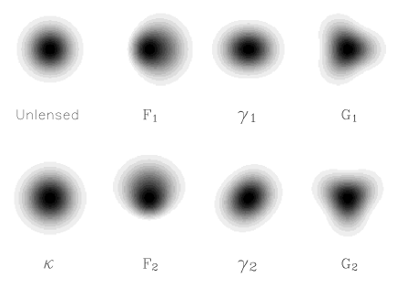
Figure 1: Weak lensing distortions with increasing spin values. Here an unlensed Gaussian galaxy with radius 1 arcsec has been distorted with 10% convergence/shear, and 0.28 arcsec^-1 flexion. Convergence is a spin-0 quantity; first flexion is spin-1; shear is spin-2; and second flexion is spin-3.

The complex formalism provides a neat way to generalize the analysis of distortions to higher orders. Taking the third derivative of the lensing potential we have the unique combinations

$${\cal F} = |{\cal F}|e^{i\phi}=\frac{1}{2}\partial\partial^{*}\partial\psi=\partial\kappa=\partial^{*}\gamma,$$

$${\cal G} = |{\cal G}|e^{i3\phi}=\frac{1}{2}\partial\partial\partial\psi=\partial\gamma,$$ (27)

where the first flexion, ${\cal F}$, is a spin-1 field and the new second flexion, ${\cal G}$, is seen to be a spin-3 field. Here $\phi$ represents the position angle determining the direction of the vector or spin-3 component. Expanding the flexions in terms of the gradients of the shear field we find

$${\cal F} = (\partial_{1}\gamma_{1}+\partial_{2}\gamma_{2})+i(\partial_{1}\gamma_{2}-\partial_{2}\gamma_{1})$$

$${\cal G} = (\partial_{1}\gamma_{1}-\partial_{2}\gamma_{2})+i(\partial_{1}\gamma_{2}+\partial_{2}\gamma_{1}),$$ (28)

where the definition of the first flexion agrees with our previous results in Section 2. These two independent fields specify the weak “arciness” of the lensed image.

The complex representation allows us to find a consistency relation between the two flexion fields,

$$\partial^{*}\partial{\cal G}=\partial\partial{\cal F},$$ (29)

which can be used as a check on measurements of ${\cal F}$ and ${\cal G}$.

We are also able to obtain a direct description of the third order lensing tensor $D_{ijk}$. Defining $\mbox{$\mathcal{F}$}=\mbox{$\mathcal{F}$}_{1}+\mathrm{i}\mbox{$\mathcal{F}$}_{2}$ and $\mbox{$\mathcal{G}$}=\mbox{$\mathcal{G}$}_{1}+\mathrm{i}\mbox{$\mathcal{G}$}_{2}$ we can then re-express $D_{ijk}$ as the sum of two terms $D_{ijk}=\mbox{$\mathcal{F}$}_{ijk}+\mbox{$\mathcal{G}$}_{ijk}$, where the first (spin-1) term is

$$\mbox{$\mathcal{F}$}_{ij1} = -\frac{1}{2}\left(\begin{array}[]{cc}3\mbox{$\mathcal{F}$}_{1}&\ \ \mbox{$\mathcal{F}$}_{2}\\ \mbox{$\mathcal{F}$}_{2}&\ \ \mbox{$\mathcal{F}$}_{1}\end{array}\right)$$ (32)

$$\mbox{$\mathcal{F}$}_{ij2} = -\frac{1}{2}\left(\begin{array}[]{cc}\mbox{$\mathcal{F}$}_{2}&\ \ \mbox{$\mathcal{F}$}_{1}\\ \mbox{$\mathcal{F}$}_{1}&\ \ 3\mbox{$\mathcal{F}$}_{2}\end{array}\right)$$ (35)

and the second (spin-3) term is

$$\mbox{$\mathcal{G}$}_{ij1} = -\frac{1}{2}\left(\begin{array}[]{cc}\mbox{$\mathcal{G}$}_{1}&\ \ \mbox{$\mathcal{G}$}_{2}\\ \mbox{$\mathcal{G}$}_{2}&\ \ -\mbox{$\mathcal{G}$}_{1}\end{array}\right)$$ (38)

$$\mbox{$\mathcal{G}$}_{ij2} = -\frac{1}{2}\left(\begin{array}[]{cc}\mbox{$\mathcal{G}$}_{2}&\ \ -\mbox{$\mathcal{G}$}_{1}\\ -\mbox{$\mathcal{G}$}_{1}&\ \ -\mbox{$\mathcal{G}$}_{2}\end{array}\right).$$ (41)

In order to obtain a visual understanding of the flexion quantities, we have used these forms for the $D_{ijk}$ matrix in terms of $\mathcal{F}$ and $\mathcal{G}$ in order to calculate how a Gaussian image is transformed by the various operations of weak lensing, according to equation (15). The results are shown in Figure 1, which displays the lensing operations in order of their spin properties. The Gaussian galaxy is given a radius (standard deviation) of 1 arcsec; while the convergence and shear imposed on the galaxy are realistic (10% in each case), the flexion is deliberately chosen to be extraordinarily large for visualisation purposes (0.28 arcsec^-1, c.f. 0.04 arcsec^-1 intrinsic rms flexion on galaxies). We immediately see the shapes induced by flexion: the first flexion leads to a (vectorial, spin-1) skewness, while the second flexion leads to a three-fold (spin-3) shape.

While the first flexion probes the local density via the gradient of the shear field, the spin-3 second flexion probes the nonlocal part of the gradient of the shear field. For example, consider a Schwarzschild lens: the first flexion is by definition zero everywhere except at the origin, as the gradient of the convergence is zero everywhere except at the origin. However, there is certainly “arciness” generated by such a lens; this is described by the second flexion. We will provide explicit expressions for the first and second flexion generated by simple mass distributions in Sections 4 and 5.

The series of lensing distortions can clearly be continued to arbitrary order by taking permutations of additional spin-raising and lowering derivatives. For instance the next order of distortion can be decomposed into three fields; a spin-4 field, $\partial\partial\partial\partial\psi$, a spin-2 field, $\partial^{*}\partial\partial\partial\psi$, and a spin-0 field, $\partial^{*}\partial^{*}\partial\partial\psi$. The $n^{th}$ order term can be decomposed into Int$(1+n/2)$ independent spin fields with spins $s=n$, $n-2$, $n-4$, $\cdots$, $0$ if $n$ is even or $\cdots 1$ if odd. Consistency relations similar to those for ${\cal F}$ and ${\cal G}$ can be found for all the higher spin fields, which can also be used to estimate the convergence field via Kaiser-Squires like relations (see Section 7).

However, in this paper we restrict ourselves to exploring the possibilities given by the first and second flexion. We will now proceed to calculate analytic expressions for both of the flexion terms for simple lens models.

4 Galaxy Halos: Circular Profiles

In this section we present flexion predictions for galaxy-galaxy lensing under the assumption of a circularly symmetric lens. This is valid for a galaxy-galaxy lensing approach where we do not reorient lens galaxies, resulting in a circularly averaged mean lens; in the following section we will consider the impact of having elliptical lenses. We consider a variety of different lens models, and show how flexion can be used to constrain them.

4.1 Flexion for the Singular Isothermal Sphere

The approximately flat rotation curves observed in galaxies can be most simply reproduced by a model density profile which scales as $\rho\propto r^{-2}$. Such a profile can be obtained by assuming a constant velocity dispersion for the dark matter throughout the halo, and so is known as the singular isothermal sphere (see e.g. Binney & Tremaine 1987). The projected surface mass density of the singular isothermal sphere (SIS) is

$$\Sigma(\xi)=\frac{\sigma^{2}_{v}}{2G\xi},$$ (42)

where $\xi$ is the distance from the centre of the lens in the projected lens plane and where $\sigma_{v}$ is the one-dimensional velocity dispersion of ‘particles’ within the gravitational potential of the mass distribution, such as stars. The dimensionless surface mass density or convergence is defined as $\kappa=\Sigma/\Sigma_{c}$, where $\Sigma_{c}$ (or the critical density) is defined as

$$\Sigma_{c}=\frac{c^{2}}{4\pi G}\frac{D_{s}}{D_{l}D_{ls}},$$ (43)

where $D_{s}$ and $D_{l}$ are the angular diameter distance to the source and lens, respectively, and $D_{ls}$ is the angular diameter distance between lens and source. Thus for the case of the simple isothermal sphere we have

$$\kappa(\theta)=\frac{\theta_{E}}{2\theta},$$ (44)

where $\theta=\xi/D_{l}$ is the angular distance from lens centre in the sky plane and where $\theta_{E}$ is the Einstein deflection angle, defined as

$$\theta_{E}=4\pi\left(\frac{\sigma_{v}}{c}\right)^{2}\frac{D_{ls}}{D_{s}}.$$ (45)

The flexion, $\mathcal{F}$, caused by the SIS at an angular vector displacement, $\theta$, from the lens centre on the sky plane is thus simply

$${\bf{\cal F}}=-\left[\frac{\theta_{E}}{2\theta^{2}}\right]e^{i\phi},$$ (46)

where $\phi$ is the position angle around the lens, and in this case also gives the direction of the flexion. The first flexion for this profile is therefore circularly symmetric and (expressed as a vector) directed radially inwards towards the lens centre, as would be expected.

Similarly, the second flexion is:

$${\cal G}=\frac{3\theta_{E}}{2\theta^{2}}e^{3i\phi}\ .$$ (47)

This has a larger maximum amplitude than the first flexion for this lens profile, fades off with the same power law index away from the lens, and oscillates around the lens as a spin-3 quantity rather than a spin-1 quantity.

4.2 Flexion and Shear Derivatives

Having considered the specific case of an isothermal sphere, we can continue more generally with power law representations of the shear around a lens:

$$\gamma=-A\theta^{-n}\ ,$$ (48)

where $A$ is a constant, $n=1$ corresponds to an isothermal sphere, $n=2$ corresponds to a point mass, and so on. In particular, one can ask whether one can better describe the arced nature of lensed objects by the flexion we have defined, or the shear derivatives themselves.

In order to answer this question, for simplicity we rotate the system such that the source lies along the $+x$ axis from the lens. We then consider what the second-order lensing amplitudes would be in a “derivative-space,” composed of the two non-zero shear derivatives:

$$\psi_{D}\equiv\left(\begin{array}[]{c}\gamma_{1,1}\\ \gamma_{2,2}\end{array}\right)=\left(\begin{array}[]{c}nA\theta^{1-n}\\ -2A\theta^{1-n}\end{array}\right).$$ (49)

In “flexion-space,” where the components are the first and second flexions, the second-order lensing amplitudes are:

$$\psi_{\mbox{$\mathcal{F}$}}\equiv\left(\begin{array}[]{c}\mbox{$\mathcal{F}$}\\ {\bf\cal G}\end{array}\right)=\left(\begin{array}[]{c}(n-2)A\theta^{1-n}\\ (n+2)A\theta^{1-n}\end{array}\right).$$ (50)

We wish to find out which is the most compact basis space. For any given distribution, this will be the one for which only one eigenstate is non-zero.

Figure 2: Second order lensing amplitudes as a function of shear power law index. The solid line shows the amplitude of the flexion coefficients, and the dashed line shows the amplitude of the derivative coefficients.

Figure 2 shows the amplitudes in each of these two spaces as a function of the shear power law index. We see that, for point sources, flexion space is the most compact approach; the signal is a pure second flexion state. For a galaxy profile with $n\simeq 1$, both spaces are almost equally efficient in describing the second order lensing. Additionally, both the flexion and derivative notations can be shown to produce 4 statistically independent terms, which, taken over an ensemble of images will all have mean zero. Moreover, within a representation, the standard deviations of the two terms due to both intrinsic variation and photon noise will be identical.

We conclude that flexion is an efficient means of describing third order lensing. For point masses it is optimal; for SIS galaxies it is as good as considering shear derivatives; and in addition the division between local and non-local components which it exclusively affords is very valuable. It also describes correctly the spin properties of the lensing.

4.3 Flexion for the Softened Isothermal Sphere

The SIS mass distribution can be modified so as to remove one feature which may not be a good physical description of dark matter halos, the divergence of $\Sigma$ for $\theta\longrightarrow 0$. One simple modification is to cut off the distribution at small distances as follows:

$$\kappa(\theta)=\frac{\theta_{E}}{2\sqrt{\theta^{2}+\theta_{c}^{2}}},$$ (51)

where $\theta_{c}$ is a core radius within which the surface mass density flattens off to a value $\kappa_{0}=\theta_{E}/2\theta_{c}$; it can be seen that the projected mass distribution behaves like the SIS for $\theta\gg\theta_{c}$. The flexion due to this distribution is

$${\cal F}=-\left[\frac{\theta_{E}}{2(\theta^{2}+\theta^{2}_{c})^{3/2}}\right]\theta e^{i\phi}\ .$$ (52)

For $\theta\gg\theta_{c}$ the flexion is approximately equal to that of the SIS. However, at small separations the flexion goes to zero, as should be expected as the convergence is tending to a maximum.

The second flexion is more complicated:

$${\cal G}=\frac{\theta_{E}}{2\theta^{3}}\left(-8\theta_{c}+\frac{3\theta^{4}+12\theta^{2}\theta_{c}^{2}+8\theta_{c}^{4}}{(\theta^{2}+\theta_{c}^{2})^{3/2}}\right)e^{3i\phi}\ ,$$ (53)

but may readily be fit to observed data, and can again be seen to reduce to the SIS second flexion when $\theta\gg\theta_{c}$ and goes to zero at the centre of the lens.

4.4 Flexion for the Navarro-Frenk-White (NFW) Density Profile

Using N-body simulations, Navarro, Frenk & White (1995, 1996, 1997) have shown that the equilibrium density profiles of cold dark matter (CDM) halos can be well fitted over two orders of magnitude in radius by the formula

$$\frac{\rho(x)}{\rho_{crit}(z)}=\frac{\Delta_{c}}{x(1+x)^{2}},$$ (54)

where the radial coordinate $x$ is the radius in units of a scaling radius $r_{s}$ such that $x\equiv r/r_{s}$, $\rho_{crit}(z)$ is the critical density for closure at the epoch of the halo, and $\Delta_{c}$ is a dimensionless scaling density. This profile describes the simulation halos accurately over a broad mass range $3\times 10^{11}<M_{200}/M_{\odot}<3\times 10^{15}$, $M_{200}$ being the total mass of the halo contained within the sphere encompassing a mean overdensity of 200 times the critical density $\rho_{crit}(z)$. The radius of this sphere, designated by $r_{200}$, is used to define a second dimensionless scaling parameter for the NFW profile, namely the concentration $c=r_{200}/r_{s}$. However, the details of the NFW definitions have been implemented in several ways in the literature; Appendix A presents further discussion of the various definitions.

A procedure for finding values of $\Delta_{c}$ and $c$ which agree with the numerical simulations is detailed by Navarro et al. (Appendix, 1997): the parameters are somewhat complicated functions of the halo redshift and $M_{200}$, along with the background cosmology. A routine (charden.f) which carries out these calculations and outputs values for these scaling parameters has been made available by Julio Navarro at http://pinot.phys.uvic.ca/j̃fn/charden.

The NFW density profile implies the following form for the dimensionless surface mass density (Bartelmann 1996):

$$\kappa(y)=2\kappa_{s}\frac{f(y)}{y^{2}-1},$$ (55)

where we define $\kappa_{s}=\rho_{crit}(z)\Delta_{c}r_{s}/\Sigma_{crit}$ and $y\equiv\xi/r_{s}$, with $\xi$ defined as for equation (42). The function $f(y)$ is given by

$$f(y)=\left\{\begin{array}[]{ll}1-\frac{2}{\sqrt{1-y^{2}}}\mathrm{arctanh}\sqrt{\frac{1-y}{1+y}}&y<1\\ 1-\frac{2}{\sqrt{y^{2}-1}}\arctan\sqrt{\frac{y-1}{y+1}}&y>1.\end{array}\right.$$ (56)

The flexion for the NFW density profile is then given by

$$\mbox{$\mathcal{F}$}\equiv\mbox{\boldmath$\nabla$}_{\theta}\kappa=\frac{\partial y}{\partial\theta}\mbox{\boldmath$\nabla$}_{y}\kappa.$$ (57)

Defining $\mathcal{F}\it_{s}\equiv\kappa_{s}D_{l}/r_{s}$ we then have

$$\mbox{$\mathcal{F}$}=-\frac{2\mathcal{F}\it_{s}}{(y^{2}-1)^{2}}\left[2yf(y)-h(y)\right]e^{i\phi}$$ (58)

with $y=\theta D_{l}/r_{s}=\theta/\theta_{s}$, and where, from equation (56),

$$h(y)=\left\{\begin{array}[]{ll}\frac{2y}{\sqrt{1-y^{2}}}\mathrm{arctanh}\sqrt{\frac{1-y}{1+y}}-\frac{1}{y}&y<1\\ \frac{2y}{\sqrt{y^{2}-1}}\arctan\sqrt{\frac{y-1}{y+1}}-\frac{1}{y}&y>1.\end{array}\right.$$ (59)

The analytical form of the second flexion can also be found, using the fact that for axially symmetric projected mass profiles the magnitude of the shear can be calculated from $|\gamma(\theta)|=\bar{\kappa}(\theta)-\kappa(\theta)$, where $\bar{\kappa}(\theta)$ is the mean surface mass density within a circle of radius $\theta$ from the lens centre (see e.g. Bartelmann & Schneider 2001). Wright & Brainerd (2000) used this method to find an expression for the magnitude of shear due to an NFW halo, and their result can be used to find the derivatives of shear $\gamma_{1,1}$, $\gamma_{1,2}$ etc. Combining these derivatives as directed by equation (28) we see that the second flexion takes the form

$$\mbox{$\mathcal{G}$}=2\mbox{$\mathcal{F}$}_{s}\left[\frac{8}{y^{3}}\ln{\frac{y}{2}}+\frac{\left(\frac{3}{y}(1-2y^{2})+g(y)\right)}{(y^{2}-1)^{2}}\right]e^{3i\phi},$$ (60)

where

$$g(y)=\left\{\begin{array}[]{ll}\left(\frac{8}{y^{3}}-\frac{20}{y}+15y\right)\frac{2}{\sqrt{1-y^{2}}}\mbox{$\mathrm{arctanh}$}\sqrt{\frac{1-y}{1+y}}&y<1\\ \left(\frac{8}{y^{3}}-\frac{20}{y}+15y\right)\frac{2}{\sqrt{y^{2}-1}}\arctan\sqrt{\frac{y-1}{y+1}}&y>1.\end{array}\right.$$ (61)

To illustrate these results, we calculate the first and second flexion signals we might expect to measure for a galaxy-sized halo with an NFW profile. We choose a lens redshift $z_{l}=0.35$ and the halo $M_{200}=1\times 10^{12}h^{-1}M_{\odot}$, this lens redshift being the median of the lens galaxy sample used by Hoekstra et al. (2004), and the mass having been found to be roughly typical for galaxy halos in weak lensing analyses by Brainerd et al. (1996) and Hoekstra et al. (2004). We also choose $D_{ls}/D_{s}=0.5$ (corresponding to a source redshift of $z_{s}\approx 0.8$) and model the lensing within a standard, flat $\Lambda$CDM cosmology, setting the present-day matter density parameter $\Omega_{m,0}=0.3$, $\Omega_{\Lambda}=0.7$, the Hubble parameter $h=0.72$ and $\sigma_{8}=0.8$.

Figure 3: Top: Logarithmic surface plot of the magnitude of first flexion due to an NFW halo of $M_{200}=1\times 10^{12}h^{-1}M_{\odot}$ at redshift $z_{lens}=0.35$. Bottom: Logarithmic surface plot of the magnitude of second flexion for the same halo.

Using these values and Navarro’s charden.f we find a concentration of $c=7.20$ and a corresponding dimensionless characteristic density $\Delta_{c}=2.03\times 10^{4}$. These values for the NFW parameters are again in good agreement with those found by Hoekstra et al. (2004) who measured $\Delta_{c}=2.4^{+1.4}_{-0.8}\times 10^{4}$ as the best fit to their sample of $\sim 10^{5}$ lenses. The resulting flexion profiles are shown in Figure 3; both flexion signals reaches a 1% effect on a $\sim 4^{\prime\prime}$ scale. We will now compare these flexion profiles with those resulting from the SIS density profile, and will then discuss the measurability of this signal with realistic survey models.

4.5 A Comparison of the NFW and SIS Flexion Results

Here we use the results from Sections 4.3 and 4.4 to compare the flexion we would expect to measure for typical galaxy-galaxy lensing observations, for the SIS and NFW cases.

Figure 4: Top: Comparison of the magnitude of first flexion due to an NFW and an SIS halo of $M_{200}=1\times 10^{12}h^{-1}M_{\odot}$ at redshift $z_{lens}=0.35$. Middle: A similar $\mathcal{F}$ comparison but this time the SIS halo has $M_{200}=1.8\times 10^{12}h^{-1}M_{\odot}$. Bottom: The magnitude of $\mathcal{G}$ for an NFW and an SIS halo of $M_{200}=1\times 10^{12}h^{-1}M_{\odot}$, where the doubling in scale of the angular separation axis highlights the larger range and amplitude of the second flexion.

The SIS scaling is very straightforward in comparison to that of the NFW halo; the Einstein radius for the SIS lens is given in terms of $M_{200}$ and the halo redshift $z_{l}$ as

$$\theta_{E}=\frac{2\pi G}{c^{2}}\frac{D_{ls}}{D_{s}}\left(\frac{800\pi\rho_{crit}(z_{l})}{3}\right)^{1/3}M^{2/3}_{200}.$$ (62)

For this comparison we use the same values for $z_{l}$, $M_{200}$ and the cosmological parameters as were used in Section 4.4, giving an Einstein radius for the SIS halo of $\theta_{E}=0.215$ arcsec.

The predicted magnitudes of $\mbox{$\mathcal{F}$}_{\rm NFW}$, $\mbox{$\mathcal{G}$}_{\rm NFW}$, $\mbox{$\mathcal{F}$}_{\rm SIS}$ and $\mbox{$\mathcal{G}$}_{\rm SIS}$, as a function of angular separation from the lensing halo on the sky, are shown in Figure 4. As could be expected the profiles show a good deal of similarity, but it is apparent that both the first and second flexions due to the SIS profile are stronger than those due to the NFW at very small separations. Since one of the important features of the NFW profile is that the density in the extreme interior of the halo varies as $\propto r^{-1}$ compared to the steeper $\propto r^{-2}$ for the SIS, this is not a surprising result.

It can be seen by comparing the lower plot of Figure 4, for which the $\theta$ axis is doubled in scale, with the upper plot, that $\mbox{$\mathcal{G}$}_{\rm NFW}$ is both stronger and longer range than $\mbox{$\mathcal{F}$}_{\rm NFW}$. Interestingly, we also note that the angular separation at which the SIS halo flexion exceeds that for the NFW halo is larger by about 5 arcsec for second flexion in relation to the first flexion. These two effects are a consequence of the non-locality of $\mathcal{G}$ as a lensing measurement when compared to the directly local $\mbox{\boldmath$\nabla$}\kappa$ measurement given by $\mathcal{F}$; for the NFW profile, $\mathcal{G}$ tends to be less steep than $\mathcal{F}$ at small $\theta$ and to die away less rapidly at larger separations.

The middle plot of Figure 4 shows another feature of the comparison between the two profiles: an SIS halo of $M_{200}=1.8\times 10^{12}h^{-1}M_{\odot}$ is practically indistinguishable from an NFW halo with $M_{200}=1\times 10^{12}h^{-1}M_{\odot}$ for first flexion measurements over galaxy-galaxy separations greater than about 5 arcsec. This is a very similar property to one found by Wright & Brainerd (2000) in a comparison of the shear profiles of SIS and NFW halos. They found that the assumption of an SIS halo profile produced systematic overestimations (by factors of up to 1.5) of the mass of NFW halos. Further work will be required to determine the dependence of this effect upon $c$ for flexion measurements as Wright & Brainerd usefully did for the case of shear.

4.6 Combined Shear and Flexion - Improving NFW Halo Parameter Constraints

Previous studies of galaxy-galaxy lensing which have aimed to constrain values of halo parameters such as $M_{200}$ or $c$ for the NFW profile (see for example Brainerd et al. 1996; Hoekstra et al. 2004, hereafter HYG04 in this section; Kleinheinrich et al. 2005) have used measurements of shear exclusively. Recently Goldberg & Bacon (2005) have shown that in many lensing scenarios the signal-to-noise ratio will be larger for the flexion than for the shear at small (but still easily measurable) angular separations between source and lens. It is therefore worthwhile considering whether combining measurements of shear and flexion might improve constraints for the halo parameters such as $c$ or $M_{200}$ derived from measurements of shear alone.

In order to do this we construct a simplified but illustrative model. We can generate mock data for a sample of lens and source galaxies such as might be available using current or forthcoming galaxy imaging surveys. We model lens halos as NFW profiles, and (as in HYG04) we assume we can scale each lensing measurement in the sample to a fiducial mass $M_{200}$ or corresponding rest-frame B-band luminosity $L_{B}$ using an observationally motivated scaling relation between the two, such as that proposed by Guzil & Seljak (2002).

In order to estimate the confidence limits we might reasonably expect from weak lensing measurements, we must consider the effect of intrinsic ellipticity and flexion of unlensed galaxies. We use values of $\gamma_{int}=0.2$ and $\mbox{$\mathcal{F}$}_{int}=0.04$ for the intrinsic shear and flexion in this model (c.f. the intrinsic flexion measured by Goldberg & Bacon 2005). Redshift errors must also be considered; we assume for this simulation that we have access to photometric redshifts for each galaxy, with an uncertainty of $\Delta z$ on each individual redshift measurement (with values assigned below for broad-band and medium-band photometric redshift surveys).

Figure 5: Estimated confidence limits on NFW halo parameters available using (dotted line) shear measurements alone, (dashed line) flexion measurements alone and (solid line) combined measurements of shear and flexion. Top: a 42 sq deg ground-based survey such as that used by Hoekstra et al. (2004). Middle: a 1700 sq deg ground-based survey. Bottom: a 0.5 sq deg space based survey.

We note (e.g. Wright & Brainerd 2000) that the strength of the shear signal due to an NFW halo varies as $\gamma_{\rm NFW}\propto D_{l}D_{ls}/D_{s}$, whereas we found in Section 4.4 that the strength of the flexion varies as $\mbox{$\mathcal{F}$}_{\rm NFW}\propto D^{2}_{l}D_{ls}/D_{s}$. We thus model the error on measurements of the shear and flexion due to redshift uncertainties by calculating errors on $D_{l}D_{ls}/D_{s}$ and $D_{l}^{2}D_{ls}/D_{s}$ by numerical integration of terms such as

$$\left\langle\left(\frac{D_{l}D_{ls}}{D_{s}}\right)^{2}\right\rangle=\int^{\infty}_{0}\mbox{$\mathrm{d}$}z_{s}^{\prime}P(z_{s}^{\prime}|z_{s})\int^{\infty}_{0}\mbox{$\mathrm{d}$}z_{l}^{\prime}P(z_{l}^{\prime}|z_{l})\frac{D^{2}_{l^{\prime}}D^{2}_{l^{\prime}s^{\prime}}}{D^{2}_{s^{\prime}}}$$ (63)

where $P(z_{l}^{\prime}|z_{l})$ and $P(z_{s}^{\prime}|z_{s})$ are the probability of measuring a redshift $z_{l}^{\prime}$ or $z_{s}^{\prime}$ for a lens or source galaxy respectively, given that its true redshift is $z_{l}$ or $z_{s}$. We model these probability distributions as Gaussians with standard deviation $\Delta z$, and assume a standard $\Lambda$CDM cosmology (as in Section 4.4). We therefore estimate the fractional error in a single measurement of shear and flexion due to redshift uncertainties (given an underlying $z_{l}$ and $z_{s}$). While the size of these fractional errors depends upon each specific lens and source redshift, for the purpose of this example we set them equal to the median lens and source redshifts for each mock sample we consider. Note that while, if we had no redshift information, there would be a large scatter in the signal caused by not knowing the geometry of the lensing, this is drastically reduced with accurate photometric redshifts and is assumed to be subdominant here.

For the fiducial virial halo mass we choose $M_{200}=1\times 10^{12}h^{-1}M_{\odot}$ (corresponding to a rest-frame L-band luminosity of $L_{B}\approx 1.2\times 10^{10}h^{-2}L_{B,\odot}$ according to the results of HYG04). We choose to model confidence limits for two ground-based surveys; one similar in size to that used by HYG04, and one covering a substantially larger area of 1700 square degrees. We also consider a deeper space-based imaging survey with far smaller area of 0.5 square degrees.

The sample of galaxies used by HYG04 was taken from $R_{c}$ band imaging of the the Red-Sequence Cluster Survey (Yee & Gladders 2002) and contained $N_{l}\sim 1.2\times 10^{5}$ lens galaxies and $N_{s}\sim 1.5\times 10^{6}$ source galaxies over a sky area of 42 sq deg. This corresponds to sky number densities of $n_{l}\approx 0.8$ arcmin^-2 for the lenses and $n_{s}\approx 10$ arcmin^-2 for the source galaxies. For the larger ground-based survey we assume the same depth, but increase the survey area to 1700 sq deg. We assume a redshift uncertainty of $\Delta z=0.1$ for each galaxy in either sample, and use the median lens and source redshifts found by HYG04 of $z_{l}=0.35$ and $z_{s}=0.53$ for both ground-based mock datasets. We set the underlying NFW lens halo concentration to $c=7.20$ as in Section 4.4.

For the mock space-based dataset we set the survey area to $0.5$ sq deg, with number densities of $n_{l}=10$ arcmin^-2 and $n_{s}=30$ arcmin^-2 due to the increased depth and quality of imaging expected for space-based results. For the redshift uncertainties we use a value of $\Delta z=0.05$ (c.f. Bacon et al. 2004 for the COMBO-17 photometric redshift survey in relation to weak lensing; Wolf et al 2001), and set $z_{l}=0.5$ and $z_{s}=1.0$. Following the predictions of Navarro et al. (1997) we model each lens halo as having a slightly smaller concentration of $c=7.02$ at this deeper redshift.

We then generate a set of mock results for the tangential shear and radial flexion, averaged over annuli around the lensing galaxies (at increasing angular separations between lens and source) for the whole ensemble of galaxies in any given survey. These mock results are made by taking the theoretical (NFW) prediction for the average shear or flexion over each annulus of angular separation and offsetting it by a Gaussian random deviate scaled to the estimated overall error for that bin.

We combine the error due to redshift errors and the intrinsic signal for a single measurement, multiplied by a factor of $1/\sqrt{N_{bin}}$ where $N_{bin}$ is the number of lens-source pairs within the annulus over which we are averaging our lensing measurements.

All that remains is to choose at what angular separations to impose the divides between annuli for averaging shear and flexion measurements. Since flexion is at its most useful on small scales, while shear signals remain strong at scales large enough for the flexion to become noise dominated, we divide up the angular scales for measurement according to a geometric binning scheme. We choose 10 annuli such that the centre of the $i$th annulus lies at an angular radius

$$r_{i}=af^{(i-1)}$$ (64)

where $a=2$ arcsec and the geometric factor $f=1.5$. In this way we describe annuli which usefully cover both small (down to 2 arcsec) and larger (up to 77 arcsec) scales of angular separation.

The resulting 68%, 90% and 95%, 2-parameter confidence intervals for NFW parameters from a maximum likelihood analysis of the three mock datasets generated using this simple model can be seen in Figure 5; it is immediately apparent that measurements of flexion may have a lot to offer galaxy-galaxy lensing studies. It is especially interesting to note that the confidence-contours derived from measurements of shear and flexion appear to be oriented at different angles in the plane, allowing the two measurables to significantly complement each other. This should perhaps not come as a surprise; whereas shear is a measure related to the projected mass density $\kappa$, the first flexion directly probes the local gradient of $\kappa$, or in this case the slope of the halo profile. We should expect therefore that flexion has the potential to significantly improve constraints on the halo concentration $c$.

It is reassuring to note from Figure 5 that the size of the 68% confidence interval we derive on the fiducial $M_{200}$ for the HYG04-like survey is in good agreement with the mass constraints found by those authors for galaxies scaled to a (slightly smaller) fiducial $L_{B}=10^{10}h^{-2}L_{B,\odot}$, namely $M_{200}=(8.4\pm 0.7\pm 0.4)\times 10^{11}h^{-1}M_{\odot}$. The second error estimate corresponds to a systematic uncertainty due to the fact that HYG04 had no actual measured redshift information from the Red-Sequence Cluster Survey (see HYG04 for details); we note that even despite this fact, their errors due to intrinsic galaxy ellipticity dominate over redshift uncertainties in their investigation of galaxy-galaxy shear, and will therefore be even less dominant for surveys with measured redshifts.

5 Galaxy Halos: Elliptical Profiles

We now discuss the more general prospect of using flexion to measure the ellipticity of lenses. When describing elliptically flattened halo mass distributions, it is often simplest to work with elliptical lens potentials, $\psi(\mbox{\boldmath$\theta$})$. Unfortunately these descriptions have some severe limitations, most notably that they produce dumbbell-shaped isodensity contours for large ellipticities and can even produce negative surface-mass densities (see Kassiola & Kovner 1993).

It is thus best to consider models where the isodensity contours of the mass distribution are elliptical, despite the increased complexity of the lens potential. The simplest generalisation of the softened isothermal sphere to an elliptical density profile can be written

$$\kappa(\theta_{1},\theta_{2})=\frac{\theta_{E}}{\displaystyle 2\sqrt{\theta^{2}_{c}+\frac{\theta^{2}_{1}}{(1+\epsilon)^{2}}+\frac{\theta^{2}_{2}}{(1-\epsilon)^{2}}}},$$ (65)

where the major axis of the elliptical isodensity contours lie along the $\theta_{1}$ axis in the sky plane, and the ellipticity $\epsilon$ is defined by the ratio of minor-to-major axes ($b$ and $a$ respectively):

$$\frac{b}{a}=\frac{1-\epsilon}{1+\epsilon}.$$ (66)

The flexion vector at $(\theta_{1},\theta_{2})$ in the sky plane is then

$$\mathcal{F} = -\frac{\theta_{E}}{\displaystyle 2\left[\theta^{2}_{c}+\frac{\theta^{2}_{1}}{(1+\epsilon)^{2}}+\frac{\theta^{2}_{2}}{(1-\epsilon)^{2}}\right]^{3/2}}$$ (67)

$$\times \left(\frac{\theta_{1}}{(1+\epsilon)^{2}}+\frac{i\theta_{2}}{(1-\epsilon)^{2}}\right).$$

We note that interestingly, $\mathcal{F}$ is no longer directed towards the centre of the lens for all $(\theta_{1},\theta_{2})$; it will in fact be centrally directed only when either $\theta_{1}$ or $\theta_{2}$ are equal to zero.

It is simple to show that the flexion vector at a point $(\theta_{1},\theta_{2})$ will be directed towards a point on the major axis of the ellipse with coordinates $(a_{int},0)$ where

$$a_{int}=\left[1-\left(\frac{1-\epsilon}{1+\epsilon}\right)^{2}\right]\theta_{1}=\left[1-\left(\frac{b}{a}\right)^{2}\right]\theta_{1}.$$ (68)

Due to the $(b/a)^{2}$ term, even relatively modest ellipticities in the density distribution cause $a_{int}$ to represent a significant fraction of $\theta_{1}$. This tendency for the flexion vector to be aimed at a point significantly off lens-centre can also be seen in Figure 6, drawn for an axis ratio of $0.67$ which may be typical of galaxy halos (see e.g. Hoekstra et al. 2004). This implies that measurements of the direction of flexion in galaxy-galaxy lensing may be able to give good further constraints on the ellipticity of dark-matter halos.

Figure 6: Flexion vector field for an elliptical isothermal density distribution with minor-to-major axis ratio of 0.67. Points in the extreme interior of the diagram have been omitted for clarity and the elliptical contours follow the logarithm of $|\mbox{$\mathcal{F}$}|$.

In order to find the second flexion, we can rewrite this elliptical isothermal profile (without softening) as follows. We begin by defining a radial term:

$$\rho\equiv\sqrt{\theta_{1}^{2}+f^{2}\theta_{2}^{2}},$$ (69)

where

$$f^{2}=(a/b)^{2},$$ (70)

with $a$ the semi-major axis and $b$ the semi-minor axis. The density profile can then be defined as:

$$\kappa=\frac{A}{\rho}.$$ (71)

For this distribution, the shear can be shown to have a very simple form:

$$\gamma_{1} =-A\frac{\cos(2\phi)}{\rho} =-A\frac{\theta_{1}^{2}-\theta_{2}^{2}}{\rho\theta^{2}},$$

$$\gamma_{2} =-A\frac{\sin(2\phi)}{\rho} =-A\frac{2\theta_{1}\theta_{2}}{\rho\theta^{2}}.$$ (72)

We may compute the derivatives of these terms in a straightforward way, and hence find the corresponding complex first and second flexion:

$$\mbox{$\mathcal{F}$}=\left(-\frac{A\theta_{1}}{\rho^{3}}\right)+i\left(-\frac{Af^{2}\theta_{2}}{\rho^{3}}\right)$$ (73)

and

$$\mbox{$\mathcal{G}$}=A\left(\frac{3\theta_{1}^{5}-\theta_{1}\theta_{2}^{4}-6\theta_{1}^{3}\theta_{2}^{2}-8f^{2}\theta_{1}\theta_{2}^{4}}{\rho^{3}\theta^{4}}\right)+$$

$$iA\left(\frac{8\theta_{1}^{4}\theta_{2}+6\theta_{1}^{2}f^{2}\theta_{2}^{3}+f^{2}\theta_{1}^{4}t-3f^{2}\theta_{2}^{5}}{\rho^{3}\theta^{4}}\right).$$ (74)

The analysis becomes simpler if we only examine the angle-averaged radial terms:

$${\cal F}_{N}=\langle-\exp(-i\phi){\cal F}\rangle=-\frac{A}{\rho\theta}$$

$${\cal G}_{N}=\langle-\exp(-3i\phi){\cal G}\rangle=\frac{3A}{\rho\theta}\ .$$ (75)

A means of measuring the ellipticity of the lens is to follow Bartelmann & Schneider (2001) and measure the quadrupole moment of the flexion field over some aperture. That is:

$$Q_{\{{\cal F},{\cal G}\}}=\int_{0}^{2\pi}d\phi\{{\cal F},{\cal G}\}\exp(2i\phi)\ .$$ (76)

Despite the other advantages in simplicity of our mass model, the evaluation of the the quadrupole moment here involves an elliptic integral. However, for relatively small ellipticities, we can expand this out as a series:

$$Q_{\cal F}=-\frac{Ae}{8\theta^{2}}\simeq\frac{e}{8}\mbox{$\mathcal{F}$}_{N}$$

$$Q_{\cal G}=\frac{3Ae}{8\theta^{2}}\simeq\frac{e}{8}\mbox{$\mathcal{G}$}_{N},$$ (77)

where $e$ is the lens ellipticity. Thus the lens ellipticity measurement from flexion incurs an $e/8$ “penalty” compared to the simple measurement of the flexion itself. Taking a typical ellipticity of $0.2$, the quadrupole estimate is $0.025$ times the S/N of the flexion, and thus we need approximately 1600 times as many pairs in order to measure the lens ellipticity effectively than to measure the convergence field. Nevertheless, flexion can clearly contribute to the question of the shape of dark matter halos around galaxies.

This concludes our examination of galaxy-galaxy flexion prospects. We will now turn to another area in which flexion can contribute significantly to studies of the dark matter distribution: that of mapping the dark matter density.

6 Mass reconstruction and substructure

In this section, we discuss how flexion can be used to reconstruct the density field of matter in order to obtain a spatial map of the matter distribution. This is clearly a valuable aspect of lensing, and is already routinely achieved using weak shear. In addition, we can obtain matter maps from flexion, which as we will see can significantly improve the signal-to-noise of the density map. We will first examine how to use flexion to obtain 2-D surface density maps of matter; we will then examine how flexion can also be used for 3-D mapping of density.

6.1 2-D Mapping

For 2-D mapping, we are able to generate maps of the projected matter density (i.e. the convergence) from both $\mathcal{F}$ and $\mathcal{G}$, following the ideology of Kaiser and Squires (1993). Starting with $\mathcal{F}$, we take the Fourier transform of the relation $\mbox{$\mathcal{F}$}_{i}=\partial_{i}\kappa$ to obtain

$$\tilde{\mbox{$\mathcal{F}$}_{1}} = -ik_{1}\tilde{\kappa}({\mn@boldsymbol{k}})$$

$$\tilde{\mbox{$\mathcal{F}$}_{2}} = -ik_{2}\tilde{\kappa}({\mn@boldsymbol{k}}).$$ (78)

We can invert both of these terms to obtain an estimate for $\tilde{\kappa}$. We add these two estimates in an optimal fashion, parameterised by the variable $a$:

$$\tilde{\kappa}=\frac{ia\tilde{\mbox{$\mathcal{F}$}_{1}}}{k_{1}}+\frac{i(1-a)\tilde{\mbox{$\mathcal{F}$}_{2}}}{k_{2}}.$$ (79)

In order to optimise the estimate, we take the mean square of this equation, which in the absence of a lensing signal will have a value determined by constant noise from intrinsic flexion. We then minimise with respect to $a$, in order to find a measurement of the $\kappa$ field with minimal noise. As a result we find the following inversion:

$$\tilde{\kappa}=\frac{ik_{1}}{k_{1}^{2}+k_{2}^{2}}\tilde{\mbox{$\mathcal{F}$}_{1}}+\frac{ik_{2}}{k_{1}^{2}+k_{2}^{2}}\tilde{\mbox{$\mathcal{F}$}_{2}}.$$ (80)

This gives us a prescription for finding the surface density of matter: we measure the flexion field, take the Fourier transform, calculate $\tilde{\kappa}$ according to this equation, and then take the inverse Fourier transform to find $\kappa$.

We can perform the same calculation for the inversion from $\mathcal{G}$ to $\kappa$. We note that the components of $\mathcal{G}$ can be written in terms of the lensing potential, $\psi$ (c.f. equation 28) as

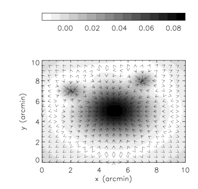
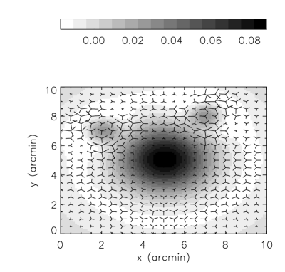
Figure 7: Shear (upper), flexion (middle) and second flexion (lower) for simulated cluster; the cluster’s convergence map is shown underlying the other weak lensing fields. Note that shear does not respond well to substructure, while the flexions respond very significantly to these regions.

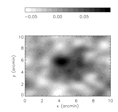
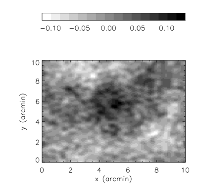
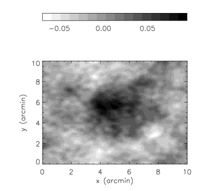
Figure 8: Recovered convergence maps from the shear alone (upper), the two flexion fields (middle) and shear and flexion combined (lower) for simulated cluster, with noise properties appropriate for a deep space-based set of observations.

$$\mbox{$\mathcal{G}$}_{1}=(\partial_{1}^{3}-3\partial_{1}\partial_{2}^{2})\psi$$

$$\mbox{$\mathcal{G}$}_{2}=(3\partial_{1}^{2}\partial_{2}-\partial_{2}^{3})\psi.$$ (81)

Hence the Fourier transform

$$\tilde{\mbox{$\mathcal{G}$}_{1}} = i(k_{1}^{3}-3k_{1}k_{2}^{2})\tilde{\psi}$$

$$\tilde{\mbox{$\mathcal{G}$}_{2}} = i(3k_{1}^{2}k_{2}-k_{2}^{3})\tilde{\psi}.$$ (82)

Again, we add these estimates of $\tilde{\psi}$ in some optimal fashion parameterised by $a$:

$$\tilde{\psi}=-\frac{ia\tilde{\mbox{$\mathcal{G}$}_{1}}}{k_{1}^{3}-3k_{1}k_{2}^{2}}-\frac{i(1-a)\tilde{\mbox{$\mathcal{G}$}_{2}}}{3k_{1}^{2}k_{2}-k_{2}^{3}}.$$ (83)

Calculating the mean square of this field and minimising with respect to $a$, we find that the optimal estimate of $\kappa$ is given by:

$$\tilde{\kappa}=i\frac{k_{1}^{3}-3k_{1}k_{2}^{2}}{(k_{1}^{2}+k_{2}^{2})^{2}}\tilde{\mbox{$\mathcal{G}$}_{1}}+i\frac{k_{2}^{3}-3k_{1}^{2}k_{2}}{(k_{1}^{2}+k_{2}^{2})^{2}}\tilde{\mbox{$\mathcal{G}$}_{2}}.$$ (84)

This provides us with the mass-mapping equations we have been seeking. We can now obtain mass maps with independent noise for $\gamma$, $\mathcal{F}$ and $\mathcal{G}$, and combine these with minimum variance weighting (with respect to noise) in order to obtain a best mass map.

These mapping relations can be efficiently expressed and trivially derived in the complex notation of Section 3 using equation (27):

$$(\kappa+iB)_{\cal F} = \partial^{-2}\partial^{*}{\cal F},$$

$$(\kappa+iB)_{\cal G} = \partial^{-4}\partial^{*}\partial^{*}\partial^{*}{\cal G}$$ (85)

where the complex part is again seen to give us the B-field component which can be used as a test of systematics. Comparing these two derivations of the mapping equations, we see that (85) gives the solution in the case of no noise, while (80) and (84) show that this is still optimal in the presence of noise due to intrinsic flexion.

The mapping process is illustrated in Figures 7 and 8. Here we have simulated a projected surface density for a toy cluster of galaxies, using a Gaussian cluster gravitational potential profile with width $\sigma=3^{\prime}$ and mean $\kappa$ within this radius of $\kappa=0.06$. We have laid down three substructure Gaussians containing 10% of the mass, with width $\sigma=1^{\prime}$ (one at the centre of the cluster). The associated shear and flexion fields shown in Figure 7 were calculated directly from equations (25) and (28). Note from this figure that the shear does not respond significantly to the small-scale structure, while flexion is most affected at these scales; this is in line with our results for galaxy-galaxy flexion, and will be explored more in the following section. We also note from the figure that the first flexion responds locally to the density gradient, whereas the second flexion responds non-locally while still giving large signals near substructure.

Shot noise is added to these fields with $\sigma_{\gamma}=0.2$, $\sigma_{\mbox{$\mathcal{F}$}}=\sigma_{\mbox{$\mathcal{G}$}}=0.04$ and projected number density $n=60$ as appropriate for a space-based survey such as GEMS (e.g. Rix et al 2004).

We have then used our inversion procedure (equations 80 and 84) together with the Kaiser-Squires inversion for shear, to obtain maps of $\kappa$ from these fields, which are displayed in Figure 8 together with a combined convergence map from all fields added with minimum variance weighting. The shear field has been smoothed with a Gaussian of radius 0.5’ as it suffers from large fluctuations on small scales, while the flexion is smoothed with radius 0.1’ as does not suffer from this problem. We note that the surface density is reconstructed well from all three fields, with maximum signal-to-noise of 3.6 for the shear reconstruction and 3.5 for the two flexion reconstructions combined. It is gratifying that the signal-to-noise for the two approaches are so similar, and strongly emphasises the value of measuring flexion as well as shear. We also note that flexion does indeed measure the substructure concentrations at the 1.4-2.6$\sigma$ level, whereas shear is not able to detect these subhalos. Future lensing maps of density will therefore benefit significantly from the inclusion of the flexion signal, especially for the purpose of charting the substructure.

6.2 3-D Mapping

We will now briefly note how to extend this method in order to map the density of matter in three dimensions with flexion, following the concepts of Taylor (2001) and Bacon & Taylor (2003). For this, we need to know what gravitational flexion we would measure upon a galaxy at any 3-D point in the Universe. We will see in the next section that the effective flexion along a line of sight over cosmological distances is given by

$$\mbox{$\mathcal{F}$}=\frac{3H_{0}^{2}\Omega_{m}^{2}}{2c^{2}}\int_{0}^{w}dw^{\prime}\frac{w^{\prime 2}(w-w^{\prime})}{a(w^{\prime})w}\frac{\partial\delta}{\partial x}$$ (86)

where $H_{0}$ is the Hubble constant, $\Omega_{m}$ is the matter density at the present epoch, $c$ is the speed of light, $w$ is comoving distance, $a$ is the expansion factor, $\delta$ is the overdensity of matter and $x$ is the transverse physical distance.

Now for a function $A(w)$ that can be written as the integral of a function $B(w^{\prime},w)$,

$$A(w)\equiv\int_{0}^{w}dw^{\prime}B(w^{\prime},w),$$ (87)

we can write the rate of change of $A$ with respect to $w$ as

$$\frac{\partial A(w)}{\partial w}=\int_{0}^{w}dw^{\prime}\frac{\partial B(w,w^{\prime})}{\partial w}+B(w,w).$$ (88)

Now $\mathcal{F}$ is in a suitable form for $A$, with $B$ given in equation (86). We can therefore use equation (88) to invert the integral for $\mathcal{F}$, and find that the transverse gradient of the matter overdensity, $\delta^{\prime}$ can be calculated in terms of the measured 3-D flexion:

$$\delta^{\prime}(w)=\frac{2c^{2}}{3H_{0}^{2}\Omega_{m}}\frac{a(w)}{w^{2}}\frac{\partial^{2}}{\partial w^{2}}(w\mbox{$\mathcal{F}$}).$$ (89)

Thus we can obtain estimates of the density gradient along a line of sight, if we have measurements of $\mbox{$\mathcal{F}$}(w)$ along that line of sight, improving signal-to-noise from 3-D maps measured using weak shear alone (Taylor et al 2004).

7 Cosmic Flexion

We now turn our attention from dark matter mapping to the overall matter distribution in the Universe. Can we use flexion to probe the distribution of large-scale structure? In order to answer this question, we carry out an analysis which is analogical to the theory of cosmic shear; here, we are trying to calculate the ‘cosmic flexion’, the flexion correlation function whose signal originates from the large-scale structure. In this section we will closely follow the analysis of Bartelmann & Schneider (2001).

7.1 Flexion Power Spectrum

If we are to find the flexion correlation function from large-scale structure, then from the definition of flexion as the gradient of the convergence, it is valuable to begin with the cosmological effective convergence, given by Bartelmann & Schneider (2001) as:

$$\kappa({\bf\theta},w)=\frac{1}{c^{2}}\int_{0}^{w}dw^{\prime}\frac{(w-w^{\prime})w^{\prime}}{w}\frac{\partial^{2}}{\partial x_{i}\partial x_{i}}\Phi[w^{\prime}{\bf\theta},w^{\prime}]$$ (90)

where ${\bf\theta}$ is the position on the sky, $w$ represents comoving distances, $x$ represents physical distances, and $\Phi$ is the gravitational potential. For simplicity, we are restricting ourselves throughout this section to a flat Universe and a flat sky approximation; for a curved sky the calculation can be extended using the formalism of Castro et al (2005). The equation above for convergence can be put into terms of the overdensity of matter using the Poisson equation

$$\frac{\partial^{2}}{\partial x_{i}\partial x_{i}}\Phi\simeq\frac{3H_{0}^{2}\Omega_{m}\delta}{2a}$$ (91)

which gives:

$$\kappa({\bf\theta},w)=\frac{3H_{0}^{2}\Omega_{m}}{2c^{2}}\int_{0}^{w}dw^{\prime}\frac{(w-w^{\prime})w^{\prime}}{w}\frac{\delta[w^{\prime}{\bf\theta},w^{\prime}]}{a(w^{\prime})}.$$ (92)

Now we wish to differentiate this to obtain a form for the effective cosmological flexion. In order to do this, we note the relationship between the required gradient with respect to angle on the sky, and the gradient of physical distances:

$$\partial_{i}=w\frac{\partial}{\partial x_{i}}.$$ (93)

Using this, we obtain for the first flexion

$$\mbox{$\mathcal{F}$}=\partial_{i}\kappa = \frac{3H_{0}^{2}\Omega_{m}}{2c^{2}}\int_{0}^{w}dw^{\prime}\frac{(w-w^{\prime})w^{\prime 2}}{a(w^{\prime})w}\frac{\partial}{\partial x_{i}}\delta[w^{\prime}{\bf\theta},w^{\prime}]$$ (94)

$$= \frac{3H_{0}^{2}\Omega_{m}}{2c^{2}}\int_{0}^{w_{H}}dw\frac{\bar{W}w^{2}}{a(w)}\delta^{\prime}[w{\bf\theta},w].$$

Here, $\delta^{\prime}$ is the transverse gradient of the overdensity, and we have defined

$$\bar{W}=\int_{w}^{w_{H}}dw^{\prime}G(w^{\prime})\frac{(w^{\prime}-w)}{w^{\prime}}$$ (95)

where $G$ is the distribution of galaxies as a function of radial distance.

Figure 9: The cosmic flexion power spectrum. Top: power spectrum as a function of angular wavenumber $l$; bottom: power spectrum per log interval in angular scale. Solid line: $(\Omega_{m}=0.3,\Omega_{\Lambda}=0.7,\sigma_{8}=0.7)$; dotted line: $(\Omega_{m}=0.3,\Omega_{\Lambda}=0.7,\sigma_{8}=0.9)$; dashed line: $(\Omega_{m}=0.2,\Omega_{\Lambda}=0.8,\sigma_{8}=0.7)$; dash-dotted line: $(\Omega_{m}=0.2,\Omega_{\Lambda}=0.8,\sigma_{8}=0.9)$.

Figure 10: Cosmic flexion correlation function for the cosmological models shown in Figure 9. Also plotted is the error on cosmic flexion for a 100 square degree ground-based survey.

In order to find the power spectrum of cosmic flexion, we will use a form of Limber’s equation, which states that if one can find two quantities $g_{1}$ and $g_{2}$ written in terms of some other quantities $q_{i}$ as

$$g_{i}=\int dw^{\prime}q_{i}(w^{\prime})G(w^{\prime})\delta^{\prime}[w^{\prime}{\bf\theta},w^{\prime}]$$ (96)

then the cross-power spectrum of $g_{1}$ and $g_{2}$ is

$$P_{12}(\ell)=\int dw^{\prime}\frac{q_{1}(w^{\prime})q_{2}(w^{\prime})}{w^{\prime 2}}P_{\delta^{\prime}}(k,w^{\prime}),$$ (97)

where $\ell$ is the angular wavenumber and $P_{\delta^{\prime}}$ is the power spectrum of the transverse gradient of the density fluctuations. We note that we can write the flexion in equation (94) in this way, with $q$ given by

$$q=\frac{3H_{0}^{2}\Omega_{m}}{2c^{2}}\frac{\bar{W}(w)w^{2}}{a(w)}.$$ (98)

Therefore we can write the flexion power spectrum as

$$P_{\mbox{$\mathcal{F}$}}(\ell)=\frac{9H_{0}^{4}\Omega_{m}^{2}}{4c^{4}}\int dw\frac{\bar{W}^{2}(w)w^{2}}{a^{2}(w)}P_{\delta^{\prime}}\left(\frac{\ell}{w},w\right).$$ (99)

Because flexion is the derivative of convergence, this power spectrum is in terms of the derivative of the overdensity. In order to describe the flexion power spectrum in terms of the more familiar overdensity itself, we note that

$$|\delta_{k}^{\prime}|^{2}=|\delta_{k}|^{2}k_{1}^{2}.$$ (100)

This implies that

$$P_{\delta^{\prime}}\left(\frac{\ell}{w},w\right)=P_{\delta}\left(\frac{\ell}{w},w\right)\frac{\ell^{2}}{w^{2}}.$$ (101)

Finally, then, we can describe the flexion power spectrum as

$$P_{\mbox{$\mathcal{F}$}}(\ell)=\frac{9H_{0}^{4}\Omega_{m}^{2}}{4c^{4}}\ell^{2}\int dw\frac{\bar{W}^{2}(w)}{a^{2}(w)}P_{\delta}\left(\frac{\ell}{w},w\right).$$ (102)

We note that this has a very similar form to the convergence power spectrum, differing only by a factor of $\ell^{2}$. Thus flexion power will be dominated by high $\ell$ components; again we see that flexion takes the form of a high-bandpass filter for density fluctuations.

One can easily show that the two-point statistics of $\mathcal{F}$ and $\mathcal{G}$ are identical; hence the first flexion power spectrum which we have calculated here is identical to the second flexion power spectrum.

From this power spectrum, we can find the flexion correlation function, as these are related by:

$$\xi_{\mbox{$\mathcal{F}$}}(\theta)=\int_{0}^{\infty}\frac{d^{2}\ell}{(2\pi)^{2}}P_{\mbox{$\mathcal{F}$}}(\ell)e^{-i{\bf\ell.\theta}}$$

$$=\int_{0}^{\infty}\frac{\ell d\ell}{2\pi}P_{\mbox{$\mathcal{F}$}}(\ell)J_{0}(\ell\theta).$$ (103)

Thus

$$\xi_{\mbox{$\mathcal{F}$}}(\theta)=\frac{9H_{0}^{4}\Omega_{m}^{2}}{4c^{4}}\int_{0}^{w_{H}}dw\frac{\bar{W}^{2}(w)w^{4}}{a^{2}(w)}$$

$$\times\int_{0}^{\infty}\frac{kdk}{2\pi}P_{\delta}(k,w)k^{2}J_{0}(kw\theta).$$ (104)

We can now examine what these predictions provide in practice. We numerically calculate the flexion power spectrum from equation (102) using the matter power spectrum prescription used in Bacon et al. (2004). This uses an initial Harrison-Zel’dovich power spectrum with non-linear evolution following Smith et al. (2003).

Figure 9 shows the flexion power spectrum in two forms. In the top panel, we present the power spectrum as a function of angular wavenumber $l$, for median redshift $z=1$. It is clear that the flexion power predictions are significantly dependent on the cosmological model; we will discuss whether this affords measurement of cosmological parameters in the context of correlation functions below. We note that the flexion power peaks at smaller angular scales than the shear power spectrum, i.e. $\sim 1$ arcmin as opposed to a few 100 arc min (c.f. Bartelmann & Schneider 2001, Figure 16). We also note that the flexion power spectrum has a very familiar shape; since the shear power spectrum is often shown premultiplied by $\ell^{2}$, the flexion power spectrum (without premultiplication by $\ell^{2}$) is identical in shape to the premultiplied shear power spectrum.

The bottom panel shows the flexion power per logarithmic interval in angular wavenumber. This shows that, for reasonable cosmological models, the power per log interval increases without limit for Smith et al (2003) density spectra. This is in contrast to the shear power spectrum, where one finds a broad maximum in power per log interval below $\simeq 1^{\prime}$ (c.f. Bartelmann & Schneider Figure 16). This again illustrates that cosmic flexion is increasingly sensitive to dark matter concentrations on small scales.

Figure 10 shows predictions for the cosmic flexion correlation function for median redshift $z=1$, where we plot flexion in units rad^-1. Note again the significantly different predictions for different cosmologies. However, we also plot errors in measuring the cosmic flexion, for a 100 square degree ground-based survey with galaxy number density of 20 arcmin^-2. Note that these error bars will have significant covariance between angular scales. We see that, while on small scales we can obtain a clear measurement of the small-scale structure, we cannot obtain measurements of the flexion in the linear density regime. This makes cosmological parameter prediction unfeasible, as it is difficult to predict amplitudes for structure on very nonlinear scales from cosmological models. Nevertheless, cosmic flexion is useful in probing these scales in order to understand them on their own terms, describing substructure and the cuspiness of halos; cosmic flexion is also complementary to cosmic shear, probing small scales in an isolated fashion, whereas cosmic shear has a broad window function for power. The cosmic flexion signal will be a useful means of testing theories of stable clustering or stable merging (c.f. Smith et al 2003).

It should be noted that in this analysis we have neglected the power that might exist from intrinsic, physical flexion correlations between galaxies. The analogous intrinsic ellipticity correlation between galaxies has been shown (e.g. Heymans et al 2004) to be small; however, further work will be necessary to measure the level of contamination of cosmic flexion due to intrinsic flexion alignments.

7.2 Convergence-Flexion Cross Power Spectrum

Figure 11: The cosmic convergence-flexion cross-power spectrum. Top: power spectrum as a function of angular wavenumber $l$; bottom: power spectrum per log interval in angular scale. The lines represent the same cosmological models as in Figure 9.

Figure 12: Cosmic convergence-flexion cross-correlation function for the cosmological models shown in Figure 9. Also plotted is the error on cosmic flexion-convergence cross-correlation for a 100 square degree ground-based survey.

In addition to the flexion power spectrum, we are also able to calculate the convergence-flexion cross power spectrum, which can easily be related to the shear-flexion cross power spectrum. We note that to do this we can again use Limber’s equation (97), but this time using $P_{\delta}$ from the outset rather than $P_{\delta^{\prime}}$. In this case, from our final power spectrum for flexion (equation 102) we see that the relevant choice of $q$ for flexion in Limber’s equation is

$$q_{\cal F}=\frac{3H_{0}^{2}\Omega_{m}\bar{W}(w)w\ell}{2c^{2}a(w)}.$$ (105)

In addition, from equation (92), we see that the choice of $q$ suitable for convergence is

$$q_{\kappa}=\frac{3H_{0}^{2}\Omega_{m}\bar{W}(w)w}{2c^{2}a(w)}.$$ (106)

Hence the cross-power spectrum between convergence and flexion can be written as

$$P_{{\cal F}\kappa}(\ell)=\frac{9H_{0}^{4}\Omega_{m}^{2}}{4c^{4}}\int dw\frac{\bar{W}^{2}(w)}{a^{2}(w)}P_{\delta}\left(\frac{\ell}{w},w\right)\ell.$$ (107)

This is shown in Figure 11, together with the associated convergence-flexion cross-correlation function in Figure 12 with appropriate errors for a 100 square degree survey. We see that this quantity has a measurement limit on an intermediate scale to shear and flexion limits ($\simeq 2^{\prime}$). It is a valuable quantity to measure, as it gives a stronger signal-to-noise than cosmic flexion, and offers a stringent check on systematic errors between the shear or convergence and flexion signals.

8 Conclusions

In this paper, we have examined how flexion can be applied to obtain both astrophysical and cosmological information. We have explored the use of galaxy-galaxy flexion to measure the mass and profile of galaxy dark matter halos; we have shown how flexion can generate maps of dark matter; and we have calculated the cosmic flexion correlation signal.

We have presented a flexion formalism, showing how the effect arises from the variation of the shear field over an object, and giving a brief discussion of how the effect can be measured using shapelets. A second flexion which was not considered in previous work has also been presented; this second flexion contains non-local information which generates arcs from point mass lenses, while the first flexion contains local information about the gradient of the density.

We have examined the efficiency of flexion as a description of second-order lensing information, in comparison with simply describing this in terms of gradients of shear. Flexion is found to be an optimal description for point mass lensing, and is about as efficient as shear gradients for singular isothermal spheres.

We have calculated flexion predictions for galaxy-galaxy lensing, for a variety of galaxy halo profiles including the singular isothermal sphere, with or without softening, the elliptical isothermal, and the NFW profile. It is found that galaxy mass can be measured well with flexion, as the mass-sheet degeneracy which plagues shear does not exist for flexion. Also, we find that by combining shear and flexion galaxy-galaxy lensing, we are able to produce powerful constraints on the halo profile.

Flexion can be used to reconstruct mass profiles directly, using a similar process to the Kaiser-Squires (1993) and Taylor (2001) inversions in 2 and 3 dimensions respectively. We have noted how flexion can act as an excellent tool for measuring substructure.

We have also calculated predictions for cosmic flexion, the flexion arising from large-scale structure. It is found that this signal is only measurable on small scales; it is useful for measuring small-scale structure and halo profiles, but will not yield independent cosmological parameters, as predictions for structure amplitudes are difficult in this highly non-linear regime.

We have seen from these applications of flexion that this quantity is a highly useful tool for a variety of methods of measuring mass fluctuations in the Universe. Flexion constitutes a valuable complement to shear, as it is sensitive where shear is not, and vice versa. With upcoming surveys from ground and space, flexion will provide a useful addition to the armoury of those who seek to understand mass in the Universe.

Appendix A NFW halo parameter conventions

We will follow the lead of Kleinheinrich et al. (2005) and briefly discuss the differing conventions used to describe NFW halos in the literature. In this comparison, and in the section above, we have adopted the convention used by Navarro et al. (1996, 1997) and by Hoekstra et al. (2004) of defining a radius $r_{200}$ from the centre of a CDM halo within which the mean density is 200 times the critical density for closure of the universe in that epoch. The mass of the halo can then be quantified via $M_{200}$, the mass contained within $r_{200}$ such that

$$M_{200}=\frac{800\pi}{3}\rho_{crit}(z)r^{3}_{200}.$$ (108)

The scaling radius $r_{s}$ of equation (54) is then expressed by Navarro et al. (1997) in terms of $r_{200}$ and another dimensionless scaling parameter, the concentration $c$, as $r_{s}=r_{200}/c$. From the definition of $M_{200}$, the parameters $c$ and $\Delta_{c}$ are linked by the relation

$$\Delta_{c}=\frac{200}{3}\frac{c^{3}}{[\ln(1+c)-c/(1+c)]}.$$ (109)

The convention outlined above is not used by all authors, with Kleinheinrich et al. (2005) choosing to define $r_{200}$ as the radius from the halo centre within which the mean density is 200 times the overall mean matter density of the universe at that epoch. This convention, which we will hereafter denote via the use of primes, thus relates $M_{200}^{\prime}$ to $r_{200}^{\prime}$ through

$$M_{200}^{\prime}=\frac{800\pi}{3}\Omega_{m}(z)\rho_{crit}(z)r_{200}^{\prime 3}$$ (110)

where $\Omega_{m}(z)$ is the matter density parameter at the epoch of the halo in question. For any given halo at a redshift $z$ we can hence define a concentration $c^{\prime}$ such that $r_{s}=r_{200}^{\prime}/c^{\prime}$ and a characteristic density related to the concentration as follows:

$$\Delta_{c}^{\prime}=\frac{200\,\Omega_{m}(z)}{3}\frac{c^{\prime 3}}{[\ln(1+c^{\prime})-c^{\prime}/(1+c^{\prime})]}.$$ (111)

We note that while $M_{200}^{\prime}$, $r_{200}^{\prime}$ and $c^{\prime}$ take different values to their unprimed counterparts, $r_{s}$ must not change and we must have $\Delta_{c}=\Delta_{c}^{\prime}$, as both these parameters describe the real physical density profile of the halo.

Given the potential for confusion of having two differing NFW conventions in the literature, it is worthwhile to describe the conversion between the two. If we have a halo of concentration $c$, defined as by Navarro et al. (1997), at a redshift $z$, then it can be quickly seen that the corresponding concentration for the primed convention is found by solving

$$\frac{\Omega_{m}(z)\,c^{\prime 3}}{[\ln(1+c^{\prime})-c^{\prime}/(1+c^{\prime})]}=\frac{c^{3}}{[\ln(1+c)-c/(1+c)]}.$$ (112)

Once $c^{\prime}$ is determined, the conversion relations for $r_{200}^{\prime}$ and $M_{200}^{\prime}$ follow trivially:

$$\frac{r_{200}^{\prime}}{r_{200}}=\frac{c^{\prime}}{c},\;\;\;\;\;\;\;\;\frac{M_{200}^{\prime}}{M_{200}}=\Omega_{m}(z)\left(\frac{c^{\prime}}{c}\right)^{3}.$$ (113)

Finally we note that in practice the primed values of $c^{\prime}$, $M_{200}^{\prime}$ and $r_{200}^{\prime}$ are somewhat larger than their unprimed counterparts.

References

- [1] Bacon D. J., Taylor A. N., 2003, MNRAS, 344, 1307.
- [2] Bacon D. J., Taylor A. N., Brown M. L., Gray M. E., Wolf C., Meisenheimer K., Dye S., Wisotzki L., Borch A., Kleinheinrich M., 2004, submitted to MNRAS, astro-ph/0403384.
- [3] Bartelmann M., 1996, A&A, 313, 697.
- [4] Bartelmann M., Schneider P., 2001, Phys. Rep., 340, 291.
- [5] Bernstein G. M., Jarvis M., 2002, AJ, 123, 583.
- [6] Binney J., Tremaine S., 1987, Galactic Dynamics. Princeton University Press, Princeton, NJ.
- [7] Brainerd T. G., Blandford R. D., Smail I., 1996, ApJ, 466, 623.
- [8] Castro P. G., Heavens A. F., Kitching T. D., 2005, submitted to Phys.Rev.D, astro-ph/0503479.
- [9] Goldberg D. M., Bacon D. J., 2005, ApJ, 619, 741.
- [10] Goldberg, D.M., Natarajan, P., 2002, ApJ, 564, 65.
- [11] Guzil J., Seljak U., 2002, MNRAS, 335, 311.
- [12] Heymans C., Brown M., Heavens A., Meisenheimer K., Taylor A., Wolf C., 2004, MNRAS, 347, 895.
- [13] Hirata C., Seljak U., 2003, MNRAS, 343, 459.
- [14] Hoekstra H., Yee H., Gladders M., 2004, ApJ, 606, 67.
- [15] Irwin J., Shmakova M., 2005, astro-ph/0504200.
- [16] Kaiser N., 2000, ApJ, 537, 555.
- [17] Kaiser N., 1995, ApJ, 439, 1.
- [18] Kaiser N., Squires G., 1993, ApJ, 404, 441.
- [19] Kaiser N., Squires G., Broadhurst T., 1995, ApJ, 449, 460.
- [20] Kassiola A., Kovner I., 1993, ApJ, 417, 450.
- [21] Kleinheinrich M., Schneider P., Rix H.-W., Erben T., Wolf C., Schirmer M., Meisenheimer K., Borch A. et al, 2004, submitted to A&A, astro-ph/0412615.
- [22] Navarro J. F., Frenk C. S., White S. D. M., 1995, MNRAS, 275, 720.
- [23] Navarro J. F., Frenk C. S., White S. D. M., 1996, ApJ, 462, 563.
- [24] Navarro J. F., Frenk C. S., White S. D. M., 1997, ApJ, 490, 493.
- [25] Refregier R., 2003, ARA&A, 41, 645.
- [26] Refregier R., 2003, MNRAS, 338, 35.
- [27] Refregier R., Bacon D., 2003, MNRAS, 338, 48.
- [28] Rix H-W., Barden M., Beckwith S. V. W., Bell E. F., Borch A., Caldwell J. A. R., Haussler B., Jahnke K. et al, 2004, ApJS, 152, 163.
- [29] Smith R. E., Peacock J. A., Jenkins A., White S. D. M., Frenk C. S., Pearce F. R., Thomas P. A., Efstathiou G., Couchman H. M. P., 2003, MNRAS, 341, 1311.
- [30] Taylor A. N., 2001, web note, astro-ph/0111605.
- [31] Taylor A. N., Bacon D. J., Gray M. E., Wolf C., Meisenheimer K., Dye S., Borch A., Kleinheinrich M., Kovacs Z., Wisotzki L., 2004, MNRAS, 353, 1176.
- [32] Van Waerbeke L., Mellier Y., astro-ph/0305089.
- [33] Wittman, D., et al. 2002, SPIE 4836, 73.
- [34] Wolf C., Meisenheimer K. & Roeser H.-J., 2001, A&A, 365, 660.
- [35] Wright C. O., Brainerd T. G., 2000, ApJ, 534, 34.
- [36] Yee H. K. C., Gladders M. D., 2002, ASP Conf. Ser. 257, 109.