The Cross-Correlation between Galaxies and Groups: Probing the Galaxy Distribution in and around Dark Matter Haloes

Abstract

We determine the cross-correlation function between galaxies and galaxy groups, using both the Two-Degree Field Galaxy Redshift Survey (2dFGRS) and the Sloan Digital Sky Survey (SDSS). Groups are identified using the halo-based group finder developed by Yang et al., which is optimized to associate those galaxies to a group that belong to the same dark matter halo. Our galaxy-group cross correlation function is therefore a surrogate for the galaxy-halo cross correlation function. We study the cross-correlation as a function of group mass, and as a function of the luminosity, stellar mass, colour, spectral type and specific star formation rate of the galaxies. All these cross-correlation functions show a clear transition from the ‘1-halo’ to the ‘2-halo’ regimes on a scale comparable to the virial radius of the groups in consideration. On scales larger than the virial radius, all cross-correlation functions are roughly parallel, consistent with the linear bias model. In particular, the large scale correlation amplitudes are higher for more massive groups, and for brighter and redder galaxies. In the ‘1-halo’ regime, the cross-correlation function depends strongly on the definition of the group center. We consider both a luminosity-weighted center (LWC) and a center defined by the location of the brightest group galaxy (BGC). With the first definition, the bright early-type galaxies in massive groups are found to be more centrally concentrated than the fainter, late-type galaxies. Using the BGC, and excluding the brightest galaxy from the cross correlation analysis, we only find significant segregation in massive groups ($M\ga 10^{13}h^{-1}\>{\rm M_{\odot}}$) for galaxies of different spectral types (or colours or specific star formation rates). In haloes with masses $\la 10^{13}h^{-1}\>{\rm M_{\odot}}$, there is a significant deficit of bright satellite galaxies. Comparing the results from the 2dFGRS with those obtained from realistic mock samples, we find that the distribution of galaxies in groups is much less concentrated than dark matter haloes predicted by the current $\Lambda$CDM model.

1 Introduction

In the standard cold dark matter (CDM) cosmogony, gravitational instability of the cosmic density field leads to the formation of virialized clumps of dark matter, called dark matter haloes, and galaxies are assumed to form in these haloes through gas cooling and condensation. One of the ultimate challenges in astrophysics is therefore to obtain a detailed understanding of how galaxies with different physical properties occupy dark matter haloes of different mass. This galaxy/dark halo connection is an imprint of various complicated physical processes governing galaxy formation, and a detailed quantification of this connection is an important key towards understanding galaxy formation and evolution within the CDM cosmogony.

To quantify the relationship between haloes and galaxies in a statistical way, one can specify the so-called halo occupation distribution, $P(N|M)$, which gives the probability to find $N$ galaxies (with some specified properties) in a halo of mass $M$. This occupation distribution can be constrained using data on the clustering properties of galaxies, as it completely specifies the galaxy bias on large scales. In the last couple of years, this approach has been used extensively to study galaxy occupation statistics and large scale structure (Jing, Mo & Börner 1998; Peacock & Smith 2000; Seljak 2000; Scoccimarro et al. 2001; Jing, Börner & Suto 2002; Berlind & Weinberg 2002; Bullock, Wechsler & Somerville 2002; Scranton 2002; Kang et al. 2002; Marinoni & Hudson 2002; Zheng et al. 2002; Magliocchetti & Porciani 2003; Berlind et al. 2003; Yang et al. 2004; Zehavi et al. 2004a,b; Zheng et al. 2004). In a series of papers, Yang, Mo & van den Bosch (2003) and van den Bosch, Yang & Mo (2003) extended this halo occupation approach by introducing the conditional luminosity function (CLF), which allows a study of the halo occupation statistics as function of galaxy luminosity and type. So far, the CLF formalism has provided a wealth of information regarding the galaxy-dark matter connection. For example, Yang et al. (2003) and van den Bosch et al. (2003) found that the halo mass-to-galaxy light ratio is a strongly non-linear function of halo mass, indicating that the star formation efficiency depends on halo mass in a complicated way. Mo et al. (2004) made predictions, based on the CLF, for the environmental dependence of the galaxy luminosity function. Croton et al. (2005) showed that these predictions are in excellent agreement with the observational data. This indicates that there is no environment dependence beyond the halo virial radius. Yang et al. (2005c), using galaxy groups identified from the Two-Degree Field Galaxy Redshift Survey (2dFGRS, Colless et al. 2001; 2003) with the halo-based group finder developed in Yang et al. (2005a), found that the halo occupation statistics derived directly from the galaxy groups are perfectly consistent with those obtained from the CLF. In particular, they found that, for a given mass, the luminosity of the central galaxy of a halo has a fairly narrow distribution, while the number of satellite galaxies roughly obeys a Poisson distribution, consistent with the subhalo statistics in numerical simulations (Kravtsov et al. 2004).

Most of the halo-occupation analyses mentioned above focused on the occupation numbers of galaxies in dark matter haloes, with little or no attention to the details regarding how these galaxies are spatially distributed within their haloes. In modeling galaxy correlation functions on small scales, the usual assumption is that the brightest halo galaxy resides (at rest) at the halo center, with the other galaxies (hereafter satellites) following a number density distribution that is identical to that of the dark matter particles. Although this assumption yields correlation functions that match the observations reasonably well, the details certainly have to be more complicated. For example, it is well known that galaxies of different types follow different spatial distributions in galaxy systems (e.g. Dressler 1980; Postman & Geller 1984; Adami, Biviano & Mazure 1998; Dominguez et al. 2001; Goto et al. 2003; Magliochetti & Porciani 2003; Madgwick et al. 2003; Scranton 2003; Collister & Lahav 2004). Red and early-type galaxies are preferentially found towards the centers of large groups.

An attractive method to probe the spatial distribution of galaxies with respect to the dark matter haloes, is to use the galaxy-halo cross-correlation function. Although dark matter haloes are not directly observable, one can use galaxy groups as a surrogate (see Yang et al. 2005a), and use the galaxy-group cross correlation function instead. Since this cross correlation function is an average of the excess of galaxies at a given distance from the group center, it can be interpreted as the average, radial distribution of galaxies both in and around their dark matter haloes. In what follows we will use the terms galaxy-halo cross correlation function and galaxy-group cross correlation function without distinction, and use the abbreviation GHCCF to indicate either one. With the large and uniform catalogues of galaxy groups that can be constructed from large galaxy redshift surveys, such as the 2dFGRS and the Sloan Digital Sky Survey (SDSS; York et al. 2000), the GHCCF can be studied as a function of group mass. Furthermore, since these redshift surveys contain information regarding various detailed properties of the individual galaxies, such as luminosity, stellar mass, colour, spectral type, star formation rate, morphological type, etc., the cross correlation technique can also be used to study the spatial distributions of galaxies in and around dark matter haloes as function of these physical properties.

In this paper, we use large catalogues of galaxy groups, extracted from the 2dFGRS and SDSS using the halo-based group finder developed by Yang et al. (2005a), to study the GHCCF as a function of luminosity, colour, spectral type, and specific star formation rate of the galaxies, and as a function of group mass. These results are used to infer the spatial distributions of different kinds of galaxies in and around dark matter haloes of different masses. The outline of this paper is as follows. In Section 2, we describe our group and galaxy catalogues. Section 3 describes how we determine the GHCCFs. Our results are presented in Section  4, and we compare the 2dFGRS observation with realistic mock galaxy redshift surveys in Section 5. Finally, we summarize our results in Section 6.

2 The Data

2.1 Group Selection

In Yang et al. (2005a; hereafter YMBJ), we developed a halo-based group finder that can successfully assign galaxies into groups according to their common haloes. The basic idea behind this group finder is similar to that of the matched filter algorithm developed by Postman et al. (1996), although it also makes use of the galaxy kinematics. The group finder starts with an assumed mass-to-light ratio to assign a tentative mass to each potential group, identified using the friends-of-friends (FOF) method. This mass is used to estimate the size and velocity dispersion of the underlying halo that hosts the group, which in turn is used to determine group membership (in redshift space). This procedure is iterated until no further changes occur in group memberships. Using detailed mock galaxy redshift surveys, the performance of our group finder has been tested in terms of completeness of true members and contamination by interlopers. The average completeness of individual groups is $\sim 90$ percent and with only $\sim 20$ percent interlopers. Furthermore, the resulting group catalogue is insensitive to the initial assumption regarding the mass-to-light ratios, and is more successful than the conventional FOF method in associating galaxies according to their common dark matter haloes.

In this paper we use this group finder to construct group catalogues from both the 2dFGRS and the SDSS, which we briefly describe below.

Table 1: Numbers of galaxies and groups in volume-limited samples.

	$z<0.09$	$z<0.13$	$z<0.18$
	(1)	(2)	(3)
Groups	2dF / SDSS	2dF / SDSS	2dF / SDSS
$12.2\leq\log M_{\rm h}<13.0$	4846 / 8994	14189 / 19615	- / -
$13.0\leq\log M_{\rm h}<13.8$	878 / 1445	2571 / 4237	- / -
$13.8\leq\log M_{\rm h}$	129 / 202	382 / 574	977 / 1619
Galaxies in 2dFGRS	early / late	early / late	early / late
$M_{b_{J}}-5\log h<-18.0$	13832 / 22754	- / -	- / -
$M_{b_{J}}-5\log h<-19.0$	7436 / 8013	23320 / 23792	- / -
$M_{b_{J}}-5\log h<-20.0$	2043 / 1277	6914 / 3835	16403 / 10361
Galaxies in SDSS	red / blue	red / blue	red / blue
$M_{r,0.1}-5\log h<-19.5$	23129 / 21626	- / -	- / -
$M_{r,0.1}-5\log h<-20.5$	7899 / 4650	21969 / 13811	- / -
$M_{r,0.1}-5\log h<-21.5$	837 / 185	2451 / 577	6583 / 1624

2.2 The 2dFGRS

We use the final, public data release from the 2dFGRS, which contains about $250,000$ galaxies with redshifts and is complete to an extinction-corrected apparent magnitude of $b_{J}\approx 19.45$ (Colless et al. 2001). The survey volume of the 2dFGRS consists of two separate declination strips in the North Galactic Pole (NGP) and the South Galactic Pole (SGP), respectively, together with 100 two-degree fields spread randomly in the southern Galactic hemisphere. For the construction of our group catalogue, we restrict ourselves only to galaxies in the NGP and SGP regions, and with redshifts $0.01\leq z\leq 0.20$, redshift quality parameter $q\geq 3$ and redshift completeness $c>0.8$. This leaves a grand total of $151,280$ galaxies with a sky coverage of $1124\,{\rm deg}^{2}$. The typical rms redshift and magnitude errors are $85\>{\rm km}\,{\rm s}^{-1}$ and $0.15$ mag, respectively (Colless et al. 2001). Absolute magnitudes for galaxies in the 2dFGRS are computed using the K-corrections of Madgwick et al. (2002).

Application of the halo-based group finder to this galaxy sample, yields a group catalogue consisting of $77,708$ systems, which in total contain $104,912$ galaxies. Among these systems, $7251$ are binaries, $2343$ are triplets, and $2502$ are systems with four members or more. The vast majority of the groups ($66,612$ systems) in our catalogue, however, consist of only a single member. Note that some faint galaxies are not assigned to any group, because it is difficult to decide whether they are the satellite galaxies of larger systems, or the central galaxies of small haloes. Detailed information regarding the clustering properties and galaxy occupation statistics of these groups can be found in Yang et al. (2005a,b,c).

As discussed in YMBJ, it is not reliable to estimate the (total) group luminosity based on the assumption that the galaxy luminosity function in groups is similar to that of field galaxies. We therefore use a more empirical approach to estimate the group luminosity $L_{18}$, defined as the total luminosity of all group members brighter than $M_{b_{J}}-5\log h=-18$. We refer the reader to Yang et al. (2005b) for details about how $L_{18}$ is estimated for each group.

As demonstrated in detail in YMBJ, $L_{18}$ is tightly correlated with the mass of the dark matter halo hosting the group, and can be used to rank galaxy groups according to halo masses. To this extent we use the mean group separation, $d=n^{-1/3}$, as a mass indicator. Here $n$ is the number density of all groups brighter (in terms of $L_{18}$) than the group in consideration. Since $L_{18}$ is tightly correlated with halo mass $M$, we can convert $d$ to $M$ (see Yang et al. 2005c for details). Unfortunately, this conversion requires knowledge of the halo mass function, and is therefore cosmology dependent. Throughout this paper we consider a $\Lambda$CDM ‘concordance’ cosmology with $\Omega_{m}=0.3$, $\Omega_{\Lambda}=0.7$, $h=0.7$ and $\sigma_{8}=0.9$.

2.3 The SDSS

We have also applied our group finder to the SDSS. Here we use the New York University Value-Added Galaxy Catalogue (NYU-VAGC) , which is described in detail in Blanton et al. (2005). The NYU-VAGC is based on the SDSS Data Release 2 (Abazajian et al. 2004), but with an independent set of significantly improved reductions. From this catalogue we select all galaxies in the Main Galaxy Sample, which has an extinction corrected Petrosian magnitude limit of $r=18$. We prune this sample to those galaxies in the redshift range $0.01\leq z\leq 0.20$ and with a redshift completeness $c>0.7$. This leaves a grand total of $184,425$ galaxies with a sky coverage of $\sim 1950\,{\rm deg}^{2}$. For SDSS galaxies, we also use stellar masses and current star formation rates released by Brinchmann et al. (2004b). The stellar masses of individual galaxies are estimated from the observed stellar absorption indices (Kauffmann et al. 2003a,b), while the current star formation rates of individual galaxies are estimated by fitting the observed spectra with spectral synthesis model (Brinchmann et al. 2004a). For the SDSS sample used in this paper, more than 90% of the galaxies have estimated stellar masses and star formation rates. We use only these galaxies to form subsamples according to stellar mass or star formation rate. We have tested that the inclusion of galaxies without stellar mass and star formation estimates does not have a significant impact on our results.

From this SDSS sample, we construct a group catalogue that contains $102,935$ systems. Among these systems, $9831$ are binaries, $3042$ are triplets, $3473$ are systems with four or more members, and the majority ($86,589$ systems) have only a single member. A more detailed description of this catalogue will be presented in Weinmann et al. (2005, in preparation). As for the 2dFGRS, we estimate the group luminosity $L_{195}$, defined as the total luminosity of all group members brighter than $M_{r,0.1}-5\log h=-19.5$. Finally, we use the rank of $L_{195}$ to assign each group a halo mass, using the same technique as described above for the 2dFGRS.

It is interesting to note that there is an overlapping region for the 2dFGRS and SDSS near the North Galactic Pole. We found 457 SDSS groups containing $\geq 3$ galaxies, among which 418 were also selected as 2dF groups. The SDSS and 2dF groups are not identical, because the selection effects are different for the two surveys, but their properties are similar.

Figure 1: The cross-correlation function, $\xi(r_{p},\pi)$, for various groups and galaxies extracted from the 2dFGRS. Panels from left to right correspond to groups of different halo masses, while panels from top to bottom correspond to galaxies with different magnitude limits (as indicated).

3 The group-galaxy cross correlation function

In redshift space, the separation between a group center and a galaxy can be split in the separations perpendicular, $r_{p}$, and parallel, $\pi$, to the line-of-sight. Explicitly, for a pair $({\bf s_{1}},{\bf s_{2}})$, with ${\bf s_{i}}=cz_{i}{\bf\hat{r}_{i}}/H_{0}$, we define

$$\pi={{\bf s}\cdot{\bf l}\over|{\bf l}|}\;,\;\;\;\;\;\;\;\;\;\;\;\;\;\;r_{p}=\sqrt{{\bf s}\cdot{\bf s}-\pi^{2}}$$ (1)

Here ${\bf l}={1\over 2}({\bf s_{1}}+{\bf s_{2}})$ is the line of sight intersecting the pair, and ${\bf s}={\bf s_{1}}-{\bf s_{2}}$. We compute the galaxy-group (or galaxy-halo) two-point cross correlation function (GHCCF), $\xi(r_{p},\pi)$, using the following estimator

$$\xi(r_{p},\pi)={N_{R}\over N_{D}}{\langle GD\rangle\over\langle GR\rangle}-1$$ (2)

where $N_{D}$, $N_{R}$ are the number of galaxies and random points, respectively, and $\langle GD\rangle$ and $\langle GR\rangle$ are the number of group-galaxy and group-random pairs with separation $(r_{p},\pi)$. Each galaxy (random point) is weighted by the inverse of the survey redshift completeness $c_{i}$.

Throughout this paper, we use volume-limited samples for both galaxies and groups. As discussed in Yang et al. (2005c), groups with given halo masses are complete only to a certain redshift. To ensure completeness, we use systems at $z\leq 0.13$ for haloes with masses in the range $12.2\leq\log M_{h}/(h^{-1}M_{\odot})<13.8$, and systems at $z\leq 0.18$ for haloes with masses in the range $13.8\leq\log M_{h}/(h^{-1}M_{\odot})$. For the galaxies, we consider three volume-limited samples corresponding to the following three redshift limits: $z=0.09$, $0.13$, $0.18$. For the 2dFGRS, these redshift limits correspond to absolute-magnitude limits $M_{b_{J}}-5\log h=-18.0$, $-19.0$, and $-20.0$, respectively, while for the SDSS, they correspond to $M_{r,0.1}-5\log h=-19.5$, $-20.5$, and $-21.5$. In Table 1, we list the number of groups and the number of galaxies in each of these volume-limited samples. When measuring the GHCCFs, we restrict galaxies and groups to the redshift range in which both the groups and galaxies are complete. To normalize the correlation function defined in equation (2), we generate a random sample that is 50 times as large as the corresponding real sample (i.e. $N_{R}=50N_{D}$).

The separations $r_{p}$ and $\pi$ are defined with respect to the group centers. Since galaxy groups have non-negligible sizes, the GHCCF can depend sensitively on how exactly the group centers are defined, especially on small scales. To probe this sensitivity, and, as we will show, to gain valuable insights, we consider two different definitions: the luminosity-weighted coordinates of the group members, and the location of the brightest galaxy in the group. In what follows we refer to these as the LW and BG centers, respectively. Note that these two definitions may give quite different results, especially for small groups with only a few members. For instance, consider a group with only two members of comparable luminosity, separated by a distance $r$. The LW center will be roughly midway between the two galaxies, while the BG center is located at one of the two galaxies. This leads to strong differences in the two-point cross correlation function. In the first case, there are two group-galaxy pairs, both with separations $\sim r/2$. In the second case, there is only one group-galaxy pair with a separation $r$; by definition, the central galaxy is at zero distance from the group center and so contributes only to the correlation function at the zero lag.

The LW and BG centers have different physical motivations and interpretations. If light traces mass, at least within dark matter haloes, the LW centers seem a natural choice. However, because of the discreteness of the galaxies, it is clear that, even when light traces mass accurately in a statistical sense, it is not necessarily an accurate description in individual systems with only a few galaxies. The BG centers are motivated by the standard picture of galaxy formation, according to which the brightest galaxy in a halo is expected to reside at rest at the halo center. If this is indeed the case, the BG centers are clearly a very physical and natural choice. Furthermore, this definition does not suffer from the discreteness of galaxies, but instead is based on it. Unfortunately, as demonstrated in van den Bosch et al. (2005b), there is strong evidence that, on average, the brightest halo galaxy has a significant offset from the center of the dark matter halo. This most likely reflects that the majority of dark matter haloes is not yet fully relaxed, implying that there is no well defined center at all. Note that this ambiguity in defining halo centers exists also for dark matter haloes in $N$-body simulations, where the center of mass and the minimum of the potential often do not coincide. Given these difficulties, we feel that the best approach is simply to use both definitions, and to see whether the differences in the resulting GHCCFs can provide new insights.

Fig. 1 shows the contours of $\xi(r_{p},\pi)$ for groups (haloes) of different masses and for galaxies of different luminosities. For conciseness, we only show the results based on the LW centers. Note that here and in the following we use volume-limited samples both for galaxies and galaxy groups. The effect of redshift space distortions is clearly visible: on small scales $\xi(r_{p},\pi)$ is stretched in the $\pi$-direction, due to the peculiar, virialized motions of galaxies within dark matter haloes. Note that this effect, often called the Finger-of-God effect, is much more pronounced in the more massive haloes (right-hand columns), reflecting their larger velocity dispersions. On large scales, the contours are squashed along the line-of-sight direction, due to the infall effect discussed by Kaiser (1987). In a separate paper (Li et al. 2005, in preparation), we model these redshift space distortions in detail, in order to infer the velocity field and mass density distribution in and around dark haloes. In what follows, we only focus on the projection of $\xi(r_{p},\pi)$ along the $\pi$-direction (i.e., the line-of-sight):

$$w_{p}(r_{p})=\int_{-\infty}^{\infty}\xi(r_{p},\pi){\rm d}\pi=2\int_{r_{p}}^{\infty}\xi(r)\,{r\,{\rm d}r\over\sqrt{r^{2}-r_{p}^{2}}}$$ (3)

The second equality shows that $w_{p}(r_{p})$ is a simple Abel transform of the real-space cross correlation function, $\xi(r)$. This owes to the overall isotropy and to the fact that the redshift-space distortions only affect $\pi$, but not $r_{p}$, and implies that $w_{p}(r_{p})$ will have a power-law shape as long as $\xi(r)$ has a power-law shape. In practice, we integrate equation (3) over the range $|\pi|\leq 40\>h^{-1}{\rm{Mpc}}$. From now on, whenever we refer to the GHCCF, we mean this projected cross-correlation function $w_{p}(r_{p})$.

Figure 2: The projected cross-correlation function between galaxies and groups in the 2dFGRS. Solid and dashed lines correspond to luminosity weighted (LW) and brightest galaxy (BG) group centers, respectively. The dotted lines illustrate the 1-halo term corresponding to an NFW profile that belongs to a halo with a mass that is equal to the median mass of the range considered. The arrows in the upper panels indicate the corresponding virial radii.

Figure 3: The ratio of the projected 2dFGRS cross-correlation function and the power-law relation of equation (5). Results are shown for three lower limits on the galaxy luminosity, as indicated (with $M^{\prime}_{b_{J}}=M_{b_{J}}-5{\rm log}h$). Upper and lower panels show the results obtained using luminosity weighted (LW) and brightest galaxy (BG) group centers, respectively. Arrows indicate the virial radii of the median-mass haloes (cf. Fig. 2). Note that in order to eliminate the impact of cosmic variance, we restrict all galaxy and group samples to the same volume with $0.01\leq z\leq 0.09$ (see text for discussion).

Figure 4: Similar to Fig 3, but for SDSS galaxies of different stellar masses. Note that these samples are also restricted to redshifts $0.01\leq z\leq 0.09$.

4 Results

4.1 The shape of the cross correlation function

Fig. 2 shows the GHCCF between galaxies and groups obtained from the 2dFGRS. The solid and dashed curves show the results obtained using the LW and BG centers, respectively. When using the LW centers, the GHCCFs clearly reveal two distinct regimes, a steep inner part and a relatively flat outer part. The transition between these two regimes occurs at a radius that is comparable to the virial radius of the haloes in consideration (indicated by arrows in the upper panels, and described in more detail below). In the terminology of the halo model (e.g., Cooray & Sheth 2002), the inner part of the GHCCF is dominated by the ‘1-halo’ term, in the sense that the galaxy-group pairs are dominated by the ones between galaxies and their own host group, while on larger scale, the GHCCF is dominated by pairs between groups and the member galaxies of other groups or of galaxies not in groups. When using the BG centers, the small scale GHCCF is significantly shallower, with no clear transition from the ‘1-halo’ to ‘2-halo’ regimes. The difference between the small scale GHCCFs based on the LW and BG centers is most pronounced in the cross correlation between low-mass groups and bright galaxies. This suggests that these groups typically contain only a single bright galaxy near their LW centers. In this case, the number of group center/galaxy pairs on small scales is greatly reduced if the central galaxies are not used in the pair count, as in the case of the BG center.

For pair separations larger than the virial radius, the exact definition of the group center is not important, and all GHCCFs are roughly parallel to each other, independent of the group mass or the galaxy luminosity function. To good approximation, this large scale GHCCFs can be described by a power law $w(r_{p})/r_{p}\propto r^{-1.6}$ (indicated by a straight line in the central panel of Fig. 2). This is in agreement with the linear halo bias model (Mo & White 1996), which states that at large (linear) scales, the real-space cross correlation function between haloes of mass $M$ and galaxies of luminosity $L$ can be written as

$$\xi_{gh}(r)=b_{g}(L)b_{h}(M)\xi_{\rm dm}(r)\,,$$ (4)

with $\xi_{\rm dm}(r)$ the dark matter correlation function, and $b_{g}(L)$ and $b_{h}(M)$ the bias of galaxies of luminosity $L$ and of haloes of mass $M$, respectively. As long as this linear bias model applies, it is therefore expected that the galaxy-halo cross correlation functions all have the same form, with a normalization that depends on the luminosities and masses of the galaxies and haloes considered.

The dotted curves in Fig. 2 show the projected correlation function obtained for NFW (Navarro, Frenk & White 1997) profiles of dark matter particles. For each of the three mass bins, we use the mean mass of the groups in consideration to estimate a ‘virial’ radius [marked as arrows; defined as the radius within which the mean overdensity is that given by the spherical collapse model], and to obtain a halo concentration parameter using the model of Eke, Navarro & Steinmetz (2001). The profile is assumed to be truncated at the ‘virial’ radius, and the projected correlation function is obtained by integrating the NFW profile along the line-of-sight. Using the LW group centers, and including faint galaxies in the group-galaxy pair counts, yields a GHCCF that roughly follows the NFW profile, except for the most massive groups where the NFW profile overpredicts the actual GHCCF. In the case of the BG centers, the ‘1-halo’ part of the GHCCF is much shallower than the NFW profile, especially for small groups. Although it is tempting to use this NFW comparison to constrain the spatial bias of galaxies within dark matter haloes, we will demonstrate in Section 5 that this comparison is not straightforward. In particular, using realistic Mock Galaxy Redshift Surveys (MGRSs), we will show that the GHCCF based on the LW centers does not reveal the actual distribution of galaxies. Therefore, the NFW comparison shown here has to be interpreted with care.

We have performed a similar analysis for the SDSS groups. Since these results are very similar to those based on the 2dFGRS groups shown in Figs. 1 and 2, we do not show them here.

Figure 5: The ratio of the projected 2dFGRS cross-correlation function and the power-law relation of equation (5) for early-type (solid lines) and late-type (dashed lines) galaxies. Thick and thin lines correspond to LW and BG centers, respectively.

Figure 6: The ratio of the projected cross-correlation function and the power-law relation of equation (5) for red (solid lines) and blue (dashed lines) galaxies in the SDSS. Thick and thin lines correspond to LW and BG centers, respectively.

4.2 Dependence on galaxy luminosity and stellar mass

Before we proceed to probe the dependence of the GHCCF on galaxy luminosity and stellar mass, we apply further restrictions to our samples. The 2dFGRS contains two gigantic super-clusters; one in the NGP at $z\sim 0.08$, and the other in the SGP at $z\sim 0.11$ (Baugh et al. 2004). The presence of such structures can affect the clustering statistics, and so care must be taken when comparing samples of different depths. In order to eliminate the impact of these extraordinary structures on our investigation, in this subsection we restrict all the galaxy and group samples to the same volume (i.e., all cut to redshift $z\leq 0.09$), and make comparisons for samples in the same volume. The choice of the cut at $z=0.09$ is a compromise between having large volume and having completeness for the faintest galaxies in consideration ($M_{b_{j}}-5\log(h)=-18$). Note that in order to have sufficient large volume for good statistics, this redshift cut still includes the supercluster at $z=0.08$.

Fig. 3 shows how the GHCCF depends on galaxy luminosity. Here we plot the ratio between the GHCCF and the following power law:

$$w_{p}(r_{p})/r_{p}=\left({r_{p}\over 10h^{-1}\>{\rm Mpc}}\right)^{-1.6}$$ (5)

As shown in Fig. 2, this power law matches the shapes of all GHCCFs on large scales. The amplitudes of the large scale GHCCFs, however, are different for different group masses and different galaxy luminosities, reflecting the mass and luminosity dependence of the halo and galaxy bias, respectively (cf., eq.[4]). As is easily inferred from Fig. 2, the halo bias $b_{h}(M)$ is an increasing function of halo mass, while the galaxy bias $b_{g}(L)$ is an increasing function of luminosity. This immediately implies that brighter galaxies are preferentially found in more massive haloes, which is the principle on which the conditional luminosity formalism is based (Yang et al. 2003, 2005c).

The behavior on scales smaller than the virial radius (i.e. the ‘1-halo’ term) is more complicated, and depends strongly on the definition of the group center. In the case of the LW centers (upper panels), bright galaxies have a steeper cross correlation on small scales than fainter galaxies. This suggests that brighter galaxies have a more concentrated radial distribution within dark matter haloes. However, if one uses the BG centers (bottom panels), so that the brightest galaxies themselves are not included in the group-galaxy pair counts, there is no significant luminosity dependence of the GHCCF in haloes with $M\ga 10^{13}h^{-1}{\rm M}_{\odot}$. This is an interesting result, because it implies that the strong luminosity segregation of galaxies observed in rich groups and clusters is almost entirely due to the brightest, central galaxy in the halo; any luminosity segregation of satellite galaxies in these systems is at best weak. For haloes with masses $M\la 10^{13}h^{-1}{\rm M}_{\odot}$ the small scale GHCCF is in fact stronger for fainter galaxies. This suggests that satellite galaxies in a low-mass halo are typically significant fainter than their brightest, central galaxy, so that there are only a few pairs of bright galaxies in these haloes. As we will show in Section 5, similar results are obtained from the MGRSs.

All results presented above are based on luminosities in the photometric $b_{J}$-band. Since the mass-to-light ratio of a galaxy in this (blue) band depends strongly on its star formation history, the lack of luminosity segregation of satellite galaxies does not necessarily mean a lack in mass segregation. To test this, we now turn to our SDSS group catalogue, where for each galaxy we also have estimates of their stellar mass and specific star formation rate (see Section 2.3).

Fig. 4 shows the GHCCFs obtained from the SDSS groups, split into two subsamples according to the stellar mass of the galaxies. The dividing mass of $\log M_{\star}=10.6$ is chosen so that the two subsamples contain roughly the same number of galaxies. Comparing the mass dependence with the luminosity dependence shown in Fig. 3 one notices an overall resemblance, indicating that, to first order, more luminous galaxies (in the blue $b_{J}$-band) are more massive. However, there are also some subtle differences. For example, whereas the small scale GHCCFs reveal no luminosity dependence for high mass haloes when using the BG centers, a small stellar mass dependence is apparent. This suggests that satellite galaxies are mildly segregated by mass. The fact that this effect is not seen when using the $b_{J}$-band luminosities may reflect that lower mass galaxies are relatively bluer. Indeed, as shown in Kauffmann et al. (2004), the specific star formation rate and stellar mass are anti-correlated.

Note also that the GHCCFs for low mass haloes on small scales are lower for more massive (in stellar mass) satellite galaxies, which is similar to the luminosity dependence shown in Fig. 3.

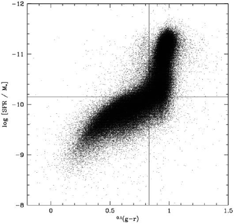
Figure 7: The colour-SSFR (specific star formation rate) relation for SDSS galaxies used in our analysis. Vertical line is the dividing line we adopted to separate galaxies into blue and red populations, while the horizontal line is the dividing line we adopted to separate galaxies into high- and low-SSFR populations. Note that these two criteria separate galaxies in approximately the same way.

4.3 Dependence on galaxy type, colour and star formation activity

Madgwick et al. (2002) used a principal component analysis of galaxy spectra taken from the 2dFGRS to obtain a spectral classification scheme for the 2dFGRS galaxies. They used the parameter $\eta$, a linear combination of the two most significant principal components, to classify galaxies into different spectral types. As shown by Madgwick et al. (2002), $\eta$ follows a bimodal distribution and can be interpreted as a measure for the current star formation rate in each galaxy. Furthermore, $\eta$ is well correlated with morphological type (Madgwick 2002). In what follows we adopt the classification suggested by Madgwick et al. and classify galaxies with $\eta<-1.4$ as ‘early-types’ and galaxies with $\eta\geq-1.4$ as ‘late-types’.

Note that in all what follows, since we are not comparing the GHCCFs in different volumes, we do not restrict the galaxy and group samples to the same volume (i.e., the cut to redshift $z\leq 0.09$). In Fig. 5, we plot the GHCCF obtained from the 2dFGRS, divided by the the power law (5), for early and late type galaxies. In all cases, the early-type galaxies have a larger correlation amplitude at scales larger than the virial radius. Since early-type galaxies are preferentially found in more massive haloes and are, on average, brighter than late-type galaxies, this simply reflects the fact that $b_{h}(M)$ and $b_{g}(L)$ are increasing functions of mass and luminosity, respectively. In haloes with masses $M\ga 10^{13}h^{-1}{\rm M}_{\odot}$ early-type galaxies tend to be more centrally concentrated, as is evident from the fact that their GHCCF on scales smaller than the halo virial radius is stronger.

This is consistent with Collister & Lahav (2004), who found that early-type galaxies in the 2dFGRS have a more concentrated profile than late-type galaxies, and dominate the number counts towards the group (halo) center. However, we find that in lower mass haloes such a trend is much weaker.

By comparing the GHCCFs obtained from the two definitions of group centers, one can see that the type segregation in haloes in the intermediate mass range is mainly caused by the central galaxies. This suggests that in haloes with masses $\sim 10^{13}h^{-1}{\rm M}_{\odot}$, early-type galaxies start to dominate the population of central galaxies. In the more massive haloes, early types continue to have a more concentrated distribution, even if central galaxies are not taken into account (i.e., when the BG centers are used). This reflects the fact that massive haloes are dominated by early-types.

As mentioned above, the spectral parameter $\eta$ can be interpreted as a measure for the current star formation activity in each galaxy. Given that star formation activity is strongly correlated with the optical colour of a galaxy, one expects to obtain similar results when splitting the sample of galaxies according to colour, rather than according to the value of $\eta$. To test this, we use the $g-r$ colours of galaxies in the SDSS. We split our sample of SDSS galaxies into two subsamples of roughly equal size, by using ${{}^{0.1}}(M_{g}-M_{r})=0.83$ as a dividing line. For the volume-limited sample used in our analysis, this dividing line is approximately the one that separates the bimodal ${{}^{0.1}}(M_{g}-M_{r})$ colour distribution. In what follows we refer to galaxies with ${{}^{0.1}}(M_{g}-M_{r})>0.83$ and ${{}^{0.1}}(M_{g}-M_{r})<0.83$ as red and blue galaxies, respectively. Note that since we are only interested in the relative color dependence of the GHCCFs, we do take account of the fact that the bimodality of the galaxy color distribution is magnitude dependent (e.g., Blanton et al. 2003b; Baldry et al. 2004; Hogg et al. 2004). Fig. 6 plots the GHCCFs between the SDSS groups and these two subsamples of galaxies. Comparing these results with those shown in Fig. 5, we see that, as expected, the colour dependence of the GHCCF is very similar to the spectral-type dependence obtained from the 2dFGRS. There are noticeable differences for the brightest samples. These differences are largely caused by the fact that the luminosity cut is higher in the brightest sample shown in Fig. 6 than that shown in Fig. 5.

We have also examined the dependence of the GHCCF on the specific star formation rate (SSFR), which we defined as the ratio between the current star formation rate and the stellar mass. For the SDSS data, both these numbers are obtained from Kauffmann et al. (2003a,b) and Brinchman et al. (2004), as discussed in Section 2.3. We used ${\log\rm SSFR}=-10.15$ to separate galaxies into high- and low-SSFR subsamples with similar galaxy numbers. The resulting GHCCFs for these subsamples are almost identical to those shown in Fig. 6 based on colour separation. To better understand the similarity in the dependence of GHCCF on SSFR and colour, we plot the SSFR-colour relation in Fig. 7. Clearly, the separation at ${\log\rm SSFR}=-10.15$ and the separation at ${{}^{0.1}}(M_{g}-M_{r})=0.83$ lead to very similar subsamples. If we separate galaxies according to their absolute star formation rate (SFR), rather than their specific star formation rate (SSFR), the difference between the high and low SFR galaxies is much weaker. This owes to the fact that massive galaxies in clusters may still have considerable amounts of ongoing star formation, even though their SSFR is low.

The results obtained above show that galaxies with low SSFRs (or red colours) are more concentrated in massive haloes than galaxies with high SSFRs (bluer colours). This may be interpreted as evidence that the SFR is suppressed once a galaxy comes close to the center of a massive halo (cluster), where the interstellar gas is striped by the hot intra-cluster medium. However, the explanation is not unique. It is also possible that more massive galaxies have lower SSFRs (due to , e.g., stronger AGN feedback), and that they are more concentrated because of dynamical friction. In this case, it is not the environment but the stellar mass that determines the SSFR of a galaxy. As we show in detail in Weinmann et al. (2005, in preparation), galaxies with larger stellar masses have, on average, lower SSFRs. This implies that the more concentrated distribution of galaxies with a low SSFR should at least partially be due to mass segregation. However, for a given stellar mass, there is also a dependence on environment, in the sense that the fraction of galaxies with low SSFRs increases as one goes from low-mass to high-mass systems, or from the outer to the inner regions in massive haloes (Weinmann et al. 2005, in preparation). This suggests that environmental effects may also play some role.

Figure 8: The projected cross-correlation function between galaxies and groups obtained from mock 2dFGRS catalogues. Solid and dashed lines correspond to luminosity weighted (LW) and brightest galaxy (BG) group centers, respectively. As in Fig. 2, the dotted lines illustrate the 1-halo term corresponding to an NFW profile that belongs to a halo with a mass that is equal to the median mass of the range considered. Errorbars are obtained from the 1-$\sigma$ variance among eight independent MGRSs, and thus reflect the expected variance due to cosmic scatter.

Figure 9: Same as Fig 8, except that the ‘1-halo’ terms are plotted separately (thin lines). In most cases, the small scale GHCCFs are dominated by the ‘1-halo’ term and the contribution of projected ‘2-halo’ pairs is negligible. The exception is the ‘1-halo’ term of the GHCCF between low mass haloes and bright galaxies (lower left panel), which is completely dominated by ‘2-halo’ pairs due to projection effects if the BG centers are used (see text for detailed discussion).

Figure 10: The ‘1-halo’ terms of the GHCCFs obtained from mock catalogues without taking into account fiber collisions and image blending. Solid and dashed lines correspond to luminosity weighted (LW) and brightest galaxy (BG) group centers, respectively. The dotted lines show the ‘1-halo’ terms of the GHCCFs obtained from projecting the NFW profiles of dark matter particles. Note that the shapes of the NFW input profiles are recovered remarkably well by the GHCCFs assuming BG centers. The difference in the amplitude between the NFW profile and the ‘1-halo’ term of the GHCCF is due to the fact that the ratio between the mean number of galaxies in a halo and the halo mass decreases with halo mass for massive haloes.

Figure 11: Comparison between the ‘1-halo’ terms of the GHCCFs obtained from the MGRSs and the 2dFGRS. Here results are shown only for BG centers. The solid lines are the results from the 2dFGRS, while the dashed and dotted lines are the results for MGRSs assuming various concentrations for the galaxy distribution in dark matter haloes, as indicated.

5 Comparison with mock catalogues

What can we learn from the above results about the distribution of galaxies in and around dark matter haloes? Unfortunately, a direct interpretation is hampered by the fact that the data used suffers from various incompleteness effects. In particular, there is a close-pair incompleteness that arises from fiber collisions and image blending (Colless et al. 2001; Cole et al. 2001; Hawkins et al. 2003; van den Bosch et al. 2005a). Obviously, such incompleteness has important impact on any pair-statistic, including the galaxy-group cross correlation studied here, and needs to be accounted for. To this extent we use detailed mock galaxy redshift surveys (hereafter MGRSs) that include all these selections and incompleteness effects as present in the real data. The procedure of including fiber collision and image blending are described in van den Bosch et al. (2005a), and we refer the reader to that paper for details. From these MGRSs we compute the same GHCCFs as for the real data, allowing for a fair, one-to-one comparison.

The MGRSs are constructed for the 2dFGRS by populating dark matter haloes in large, numerical $N$-body simulations, with galaxies of different luminosities. To decide what galaxy to put in what halo, we use the conditional luminosity function, which assures that the entire population of galaxies has the correct luminosity function and clustering properties (as function of luminosity). Within each individual halo, we can modify the spatial distribution of galaxies and investigate how this impacts on the ‘observed’ GHCCF. Our MGRSs are tailored to resemble the 2dFGRS as close as possible, taking detailed account of the various selection and incompleteness effects. A detailed description of the MGRS construction is given in the Appendix, and, in more detail, in Yang et al. (2004) and van den Bosch et al. (2005a). Note that these MGRSs have also been used in YMBJ to test and calibrate the halo-based group finder used to construct our group catalogues.

Fig. 8 shows the GHCCFs obtained from the MGRSs. A comparison with Fig. 2 shows that these are very similar to those obtained from the 2dFGRS. In particular, the GHCCF between low-mass groups and bright galaxies is, in both cases, much shallower than the NFW profile if the BG are used as group centers. Note that in the MGRSs, the brightest halo galaxy is located at the halo center, while the radial number density distribution of the satellite galaxies follows that of the dark matter particles (see Appendix).

Before we proceed to interpret the GHCCFs obtained from the MGRSs and compare these with those obtained from the 2dFGRS, we address how the GHCCF on small scales is related to the galaxy distribution in dark matter haloes. In addition to the observational selection bias, such as fiber collision and image blending, there are a number of other effects that may complicate the results of the observed GHCCF. Firstly, the projected GHCCF may be contaminated by ‘2-halo’ pairs due to projection. Secondly, our group finder cannot be perfect, and contaminations can arise because of interlopers. Finally, since different definitions of group center can lead to different GHCCF, it is necessary to know which definition should be used in order to extract information about the profile of galaxy distribution in dark matter haloes. With our realistic MGRSs, we can quantify all these effects in detail.

In order to check the importance of projection effect, we estimate the GHCCF functions using only ‘1-halo’ pairs and compare the results with the corresponding results using both ‘1-halo’ and ‘2-halo’ pairs. The results are shown in Fig. 9. In most cases, the GHCCF on small scale is dominated by the ‘1-halo’ term, and the contamination by the projected ‘2-halo’ pairs is negligible. However, if BG centers are used, the GHCCF between small haloes and bright galaxies is small, because most of the satellite galaxies in low-mass haloes are faint. In this case, the contribution by the projected ‘2-halo’ pairs becomes dominant (see the lower-left panel in Fig. 9).

As mentioned above, our mock samples include fiber collisions and image blending. It is interesting to see how big such effects are. To do this, we have generated mock samples that do not include fiber collisions and image blending, and made comparisons between the GHCCFs obtained from such samples with those in Fig. 9. We found that, for small radius where the effect is the largest, fiber collisions and image blending reduce the GHCCF by about 10% if LW centers are used, while the reduction is as large as 40% in massive haloes if BG centers are used. The effect is bigger for early-type galaxies in massive haloes, presumably because these galaxies have a more concentrated distribution.

In the MGRSs used here, the distribution of satellite galaxies in individual haloes is assumed to follow the NFW profile. In order to examine to which extent this input profile can be recovered from the GHCCF, we use mock catalogues without taking into account fiber collisions and image blending. The results are shown in Fig. 10. As mentioned above, if only bright galaxies are used, the galaxy density profile cannot be measured well for small groups. In order to sample the density profile reliably, we need to include faint galaxies. In the results shown in Fig. 10, all galaxies with $M_{b_{J}}-5\log h<-18.0$ are used. As one can see, the input profile can be reproduced. The reproduction is better with the BG centers, which is consistent with the fact that in our MGRSs central galaxies do not sample the density profile.

It should be pointed out that the MGRSs used above all assume that the brightest galaxy in a halo is sitting still at the center of the halo. As discussed in van den Bosch et al. (2005b), such assumption may not be correct. In order to investigate the impact of the phase-space distribution of the brightest galaxies in the dark matter haloes, we have also measured the GHCCFs for the MGRSs ${\rm M}_{0.0}$, ${\rm M}_{0.5}$ and ${\rm M}_{1.0}$ in van den Bosch et al. (2005b). In ${\rm M}_{0.5}$ and ${\rm M}_{1.0}$, the brightest galaxies are not sitting still at the center of the dark matter haloes, but have both velocity bias and spatial offset. The velocity bias, defined as $b_{vel}=\langle\sigma_{\rm cen}\rangle/\langle\sigma_{\rm sat}\rangle$, and spatial offset, defined as $b_{rad}=\langle r_{\rm cen}\rangle/\langle r_{\rm sat}\rangle$, for these two models are $(b_{\rm vel},b_{\rm rad})=(0.5,0.072)$ and $(1.0,1.0)$, respectively. Model ${\rm M}_{0.0}$ has $(b_{\rm vel},b_{\rm rad})=(0,0)$, and is used for comparison. We found that, if LW centers are used, the velocity bias and spatial offset have negligible impact on the GHCCF. Using BG centers, the results for ${\rm M}_{0.0}$ and ${\rm M}_{0.5}$ are similar, implying that velocity bias does not affect the GHCCF significantly, but model ${\rm M}_{1.0}$ predicts a shallower GHCCF on small scale, especially for massive haloes. In ${\rm M}_{1.0}$, the brightest galaxies have the same spatial distribution as other galaxies, and so the GHCCF on small scale is an average of the profiles around all member galaxies. As shown in van den Bosch et al. (2005b), observations based on groups selected from the 2dFGRS and the SDSS are best described by model ${\rm M}_{0.5}$, and ${\rm M}_{1.0}$ can be ruled out at high confidence level. Thus, the impact of the phase-space distribution of the brightest galaxies on the GHCCF is expected to be unimportant.

With the above tests, we are now in a position to compare our observational results with the predictions of the MGRSs. Comparing the GHCCFs obtained from the 2dFGRS (Fig. 2) with those obtained from the MGRSs (Fig. 8), one notices that the former is shallower than the latter in massive groups. Note that the MGRSs have taken account of the effects due to fiber collisions and image blending. Therefore, this discrepancy cannot be due to these effects. This suggests that, in the $\Lambda$CDM concordance cosmology considered here, the distribution of galaxies is less centrally concentrated than that of dark matter particles. In order to quantify this discrepancy, we generate MGRSs in which the radial number density distribution of satellite galaxies has a concentration that differs from that of their dark matter haloes. The results are shown in Fig. 11, together with the 2dFGRS results. It is clear that, in order to match the 2dFGRS data, the concentration $c_{\rm g}$ of the distribution of galaxies has to be lower than that of the dark matter haloes ($c_{\rm m}$) by about a factor of three. Note that the amplitude of the GHCCF obtained from the MGRS for massive haloes is higher than observed. This owes to the fact that massive groups in the MGRSs used are too rich (see Yang et al. 2005a). As discussed in Yang et al., this discrepancy can be alleviated by either taking $\sigma_{8}\simeq 0.7$ (as opposed to $0.9$ as assumed here), or by considering mass-to-light ratios of massive haloes that are much higher than what observations seem to suggest. Reducing the value of $\sigma_{8}$ has the additional advantage that is lowers the typical halo concentration of dark matter haloes, leading to a smaller difference between the concentration of dark matter haloes and that of their galaxy distribution. However, the change is only about $40\%$, which is insufficient to reach the low concentrations obtained for the galaxy distribution. We therefore conclude that in the standard $\Lambda$CDM cosmology, the distribution of galaxies in massive dark matter haloes must be less concentrated than that of the dark matter.

Using our MGRSs, we have determined, for each of the three ranges in halo mass the concentration parameters of the galaxy distributions that best match the GHCCFs of the 2dFGRS. In addition we perform this test separately for the early- and late-type galaxies (classified according to the spectral parameter $\eta$). Results are shown in Table 2, where we list the resulting values of $c_{\rm g}$. As expected, the distribution of early-type galaxies is more centrally concentrated than that of late-type galaxies. These results are in qualitative agreement with those of Collister & Lahav (2004, hereafter CL04) and Lin et al. (2004). Using clusters selected from the 2 Micron All-Sky Survey (Jarrett 2000), Lin et al. (2004) found a concentration parameter of $2.9\pm 0.2$ for the distribution of galaxies in clusters, in good agreement with our result for massive haloes. Using 2dFGRS groups selected by Eke et al. (2004), CL04 obtained the concentration of the distribution of galaxies of different types. Their results are included in Table 2 for comparison. Note that the CL04 results are averages for all groups that contain more than two galaxies, rather than for groups in a given mass range. There are also other differences between CL04’s analysis and ours. First of all, the group catalogue used by CL04 is different from ours. Although both are selected from the 2dFGRS, Yang et al. (2005a) have shown that the groups in the Eke et al. catalogue are systematically richer than those selected by our halo-based group finder. Secondly, while our results are obtained by matching observations with mock catalogues that incorporate observational selection effects, the results of CL04 were obtained by fitting the observed density profiles directly with the NFW profile. However, apart from all these differences, our results and those of CL04 are consistent with each other, both indicating that the distribution of galaxies is less concentrated than that of the dark matter.

Table 2: The concentration parameters of the distribution of galaxies ($c_{\rm g}$) and dark matter particles ($c_{\rm m}$). Columns (1), (2), and (3) list the results for haloes with masses ($\log M_{\rm h}/(h^{-1}{\rm M}_{\odot})\geq 13.8$), ($13.8>\log M_{\rm h}/(h^{-1}{\rm M}_{\odot})\geq 13.0$), and ($13.0>\log M_{\rm h}/(h^{-1}{\rm M}_{\odot})\geq 12.2$), respectively. For comparison, column (4) lists the results obtained by Collister & Lahav (2004).

	$M_{\rm h,1}$	$M_{\rm h,2}$	$M_{\rm h,3}$	CL04
	(1)	(2)	(3)	(4)
All galaxies	2.4	2.9	3.3	$2.4\pm 0.2$
Red	2.5	3.4	4.0	$3.9\pm 0.5$
Blue	1.1	1.7	2.2	$1.3\pm 0.2$
Dark Matter	7.1	8.6	10.0

6 Summary

In order to probe the spatial distribution of galaxies in and around dark matter haloes, we measured the GHCCFs between galaxies and groups (haloes) for both the 2dFGRS and the SDSS. The corresponding group catalogues are constructed using the halo-based group finder developed in Yang et al. (2005a). The resulting GHCCFs show a clear transition from the ‘1-halo’ to the ‘2-halo’ terms at around the halo virial radius. The ‘1-halo’ term measures the correlation between the group center and the galaxies that are part of that group (i.e., it measures the radial distribution of galaxies within their parent haloes), while the ‘2-halo’ term measures the large scale correlation between galaxies that reside in different parent haloes. We have used two different definitions for the group center in our estimation of the GHCCF; one is the average, luminosity weighted (LW) location of the member galaxies and the other is the location of the brightest galaxy (BG) in the group. The GHCCFs of these two definitions are almost identical on large scales (‘2-halo’ term), but very different on small scales (‘1-halo’ term). The small scale GHCCF for the BG centers is always shallower than that obtained using the LW centers, especially when cross correlating bright galaxies and low mass haloes. This indicates that the brightest galaxies in small haloes play an important, dominant role in the overall galaxy distribution profile.

We have studied the GHCCFs as a function of group mass and various properties of the galaxies (luminosity, stellar mass, colour, spectral type, and specific star formation rate). Overall, more massive groups reveal a stronger GHCCF than low mass groups. On large scales, the GHCCF is stronger for galaxies that are more luminous, more massive, red, early-type and/or with a low SSFR. All these trends can be understood in terms of the mean bias of their host haloes (i.e., more massive haloes are more strongly biased). When using the LW group centers, the GHCCFs of these same galaxies are much stronger and steeper than for their counterparts, especially in massive haloes ($M\ga 10^{13}h^{-1}M_{\odot}$). However, when the BG centers are used instead, the ‘1-halo’ term of the GHCCF does not show any clear luminosity segregation. This implies that the strong luminosity segregation of galaxies observed in rich groups is almost entirely due to their brightest central galaxy.

We compared the GHCCFs obtained from the 2dFGRS with those obtained from detailed mock galaxy redshift surveys (MGRSs) that were constructed to accurately mimic the actual 2dFGRS. The overall behavior of the GHCCFs obtained from the MGRSs is similar to that obtained from the 2dFGRS, except that the GHCCFs of the MGRSs have steeper small scale (‘1-halo’ term) profiles than observed. By carefully comparing the 2dFGRS results with a set of MGRSs, we determined the concentration parameters for the distribution of galaxies (of different types) in haloes of different masses. In qualitative agreement with Collister & Lahav (2004) and Lin et al. (2004) we find that the distribution of galaxies in dark matter haloes is significantly less concentrated than that of the dark matter particles as predicted by the standard $\Lambda$CDM model.

Appendix A Mock Galaxy Redshift Surveys

We construct MGRSs by populating dark matter haloes with galaxies of different luminosities. The distribution of dark matter haloes is obtained from a set of large $N$-body simulations (dark matter only) for a $\Lambda$CDM ‘concordance’ cosmology with $\Omega_{m}=0.3$, $\Omega_{\Lambda}=0.7$, $h=0.7$ and $\sigma_{8}=0.9$. In this paper we use two simulations with $N=512^{3}$ particles each, which are described in more detail in Jing & Suto (2002). The simulations have periodic boundary conditions and box sizes of $L_{\rm box}=100h^{-1}\>{\rm Mpc}$ (hereafter $L_{100}$) and $L_{\rm box}=300h^{-1}\>{\rm Mpc}$ (hereafter $L_{300}$). We follow Yang et al. (2004) and replicate the $L_{300}$ box on a $4\times 4\times 4$ grid. The central $2\times 2\times 2$ boxes, are replaced by a stack of $6\times 6\times 6$ $L_{100}$ boxes, and the virtual observer is placed at the center (see Fig. 11 in Yang et al. 2004). This stacking geometry circumvents incompleteness problems in the mock survey due to insufficient mass resolution of the $L_{300}$ simulations, and allows us to reach the desired depth of $z_{\rm max}=0.20$ in all directions.

Dark matter haloes are identified using the standard FOF algorithm with a linking length of $0.2$ times the mean inter-particle separation. Unbound haloes and haloes with less than 10 particles are removed from the sample. In Yang et al. (2004) we have shown that the resulting halo mass functions are in excellent agreement with the analytical halo mass function of Sheth, Mo & Tormen (2001).

In order to populate the dark matter haloes with galaxies of different luminosities, we use the conditional luminosity function (hereafter CLF), $\Phi(L|M)$, which gives the average number of galaxies of luminosity $L$ that resides in a halo of mass $M$. As demonstrated in Yang, Mo & van den Bosch (2003) and van den Bosch, Yang & Mo (2003), the CLF is well constrained by the galaxy luminosity function and by the galaxy-galaxy correlation lengths as function of luminosity. In the MGRSs used here we use the CLF with ID # 6 given in Table 1 of van den Bosch et al. (2005a). We have tested that none of our results depend significantly on this particular choice for the CLF.

Because of the mass resolution of the simulations and because of the completeness limit of the 2dFGRS, we adopt a minimum galaxy luminosity of $L_{\rm min}=10^{7}h^{-2}\>{\rm L_{\odot}}$. The mean number of galaxies with $L\geq L_{\rm min}$ that resides in a halo of mass $M$ is given by

$$\langle N\rangle_{M}=\int_{L_{\rm min}}^{\infty}\Phi(L|M)\,{\rm d}L$$ (6)

In order to Monte-Carlo sample occupation numbers for individual haloes, one requires the full probability distribution $P(N|M)$ (with $N$ an integer) of which $\langle N\rangle_{M}$ gives the mean. We differentiate between satellite galaxies and central galaxies. The total number of galaxies per halo is the sum of $N_{\rm cen}$, the number of central galaxies which is either one or zero, and $N_{\rm sat}$, the (unlimited) number of satellite galaxies. We assume that $N_{\rm sat}$ follows a Poisson distribution and require that $N_{\rm sat}=0$ whenever $N_{\rm cen}=0$. The halo occupation distribution is thus specified as follows: if $\langle N\rangle_{M}\leq 1$ then $N_{\rm sat}=0$ and $N_{\rm cen}$ is either zero (with probability $P=1-\langle N\rangle_{M}$) or one (with probability $P=\langle N\rangle_{M}$). If $\langle N\rangle_{M}>1$ then $N_{\rm cen}=1$ and $N_{\rm sat}$ is drawn from a Poisson distribution with a mean of $\langle N\rangle_{M}-1$.

We follow Yang et al. (2004) and draw the luminosity of the brightest galaxy in each halo from $\Phi(L|M)$ using the restriction that $L>L_{1}$ with $L_{1}$ defined by

$$\int_{L_{1}}^{\infty}\Phi(L|M)dL=1\,.$$ (7)

The luminosities of the satellite galaxies are also drawn from $\Phi(L|M)$, but with the restriction $L_{\rm min}<L<L_{1}$.

The positions and velocities of the galaxies with respect to the halo center-of-mass are drawn assuming that the brightest galaxy in each halo resides at rest at the center. The satellite galaxies follow a number density distribution that is identical to that of the dark matter particles, and are assumed to be in isotropic equilibrium within the dark matter potential. To construct MGRSs we use the same selection criteria and observational biases as in the 2dFGRS, making detailed use of the survey masks provided by the 2dFGRS team (Colless et al. 2001; Norberg et al. 2002). The various steps involved in this process are described in detail in van den Bosch et al. (2005b). The final MGRSs accurately match the clustering properties, the apparent magnitude distribution and the redshift distribution of the 2dFGRS, and mimic all the various incompleteness effects, allowing for a direct, one-to-one comparison with the true 2dFGRS.

Using a set of independent numerical simulations, we construct 8 independent MGRSs which we use to address scatter due to cosmic variance. Finally, for each MGRS we construct group samples using the same halo-based group finder and the same group selection criteria as for the 2dFGRS. These are used to compute the GHCCFs, as described in Section 3. The comparison with the 2dFGRS cross correlation functions is discussed in Section 5.

References

- [] Abazajian K., et al., 2004, AJ, 128, 502
- [] Adami C., Biviano A., Mazure A., 1998, A&A , 331, 439
- [] Baldry I.K., Glazebrook K., Brinkmann J., Ivezic̃ Z̃., Lupton R.H., Nichol R., Szalay A.S., 2004, ApJ, 600, 681
- [] Baugh C.M., et al., 2004, MNRAS, 351, L44
- [] Berlind A.A., Weinberg D.H., 2002, ApJ, 575, 587
- [] Berlind A.A., et al. , 2003, ApJ, 593, 1
- [] Blanton M.R., et al., 2003a, ApJ, 592, 819
- [] Blanton M.R., et al., 2003b, ApJ, 594, 186
- [] Blanton M.R., et al., 2005, AJ, 129, 2562
- [] Brinchmann J., Charlot S., White S.D.M., Tremonti C., Kauffmann G.,, Heckman T.M., Brinkmann J. 2004a, MNRAS, 351, 1151
- [] Brinchmann J., Charlot S., Heckman T.M., Kauffmann G., Tremonti C., White S.D.M., 2004b, preprint (astro-ph/0406220)
- [] Bullock J.S., Wechsler, R.H., Somerville R.S., 2002, MNRAS, 329, 246
- [] Cole S., The 2dFGRS team, 2001, MNRAS, 326, 255
- [] Colless M., et al., 2001, MNRAS, 328, 1039
- [] Colless M., et al., 2003, reprint (astro-ph/0306581)
- [] Collister A.A., Lahav O., 2004, preprint (astro-ph/0412516)
- [] Cooray A., Sheth R., 2002, Phys. Rep., 372, 1
- [] Croton D.J., et al., 2005, MNRAS, 356, 1155
- [] Dressler A., 1980, ApJ, 236, 351
- [] Dominguez M., Muriel H., Lambas D.G., 2001, ApJ, 121 1266
- [] Eke V.R., Navarro J.F., Steinmetz M., 2001, ApJ, 554, 114
- [] Eke V.R., et al., 2004, MNRAS, 348, 866
- [] Goto T., Yamauchi C., Fujita Y., Okamura S., Sekiguchi M., Smail I., Bernardi M., Gomez P. L., 2003, MNRAS, 346, 601
- [] Hawkins E., et al., 2003, MNRAS, 346, 78
- [] Hogg D.W., et al. , 2004, ApJ, 601, L29
- [] Jarrett T.H., Chester T., Cutri R., Schneider S., Skrutskie M., Huchra J.P., AJ, 119, 2498
- [] Jing Y.P., Mo H.J., Börner G., 1998, ApJ, 494, 1
- [] Jing Y.P., Börner G., Suto Y., 2002, ApJ, 564, 15
- [] Kaiser N., 1987, MNRAS, 227, 1
- [] Kang X., Jing Y.P., Mo H.J., Börner G., 2002, MNRAS, 336, 892
- [] Kauffmann G., et al. , 2003a, MNRAS, 341, 33
- [] Kauffmann G., et al. , 2003b, MNRAS, 341, 54
- [] Kauffmann G., White S.D.M., Heckman T.M., Menard B., Brinchmann J., Charlot S., Tremonti C., Brinkmann J. 2004, MNRAS, 353, 713
- [] Kravtsov A.V., Berlind A.A., Wechsler R.H., Klypin A.A., Gottlöber S., Allgood B., Primack J.R., 2004, ApJ, 609, 35
- [] Lin Y.T., Mohr J.J., Stanford S.A., 2004, ApJ, 610, 745
- [] Madgwick D.S., et al., 2002, MNRAS, 333, 133
- [] Madgwick D.S. et al. , 2003, MNRAS, 344, 847
- [] Magliocchetti M., Porciani C., 2003, MNRAS, 346, 186
- [] Marinoni C., Hudson M.J., 2002, ApJ, 569, 101
- [] Mo H.J., White S.D.M, 1996, MNRAS, 282, 347
- [] Mo H.J., Yang X.H., van den Bosch F.C., Jing Y.P., 2004, MNRAS, 349, 205
- [] Navarro J.F., Frenk C.S., White S.D.M., 1997, ApJ, 490, 493
- [] Norberg P., et al., 2002, MNRAS, 332, 827
- [] Peacock J.A., Smith R.E., 2000, MNRAS, 318, 1144
- [] Postman M., Geller M.J., 1984, ApJ, 281, 95
- [1996] Postman M., et al., 1996, AJ, 111, 615
- [] Scoccimarro R., Sheth R.K., Hui L., Jain B., 2001, ApJ, 546, 20
- [] Scranton R., 2002, MNRAS, 332, 697
- [] Scranton R., 2003, MNRAS, 339, 410
- [] Seljak U.,2000, MNRAS, 318, 203
- [] Sheth R.K., Mo H.J., Tormen G., 2001, MNRAS, 323, 1
- [] van den Bosch F.C., Yang X., Mo H.J., 2003, MNRAS, 340, 771
- [] van den Bosch F.C., Norberg P., Mo H.J., Yang X., 2004, MNRAS, 352, 1302
- [] van den Bosch F.C., Yang X., Mo H.J., Norberg P., 2005a, MNRAS, 356, 1233
- [] van den Bosch F.C., Weinmann S.M., Yang X., Mo H.J. Li C., Jing Y.P., 2005b, preprint (astro-ph/0502466)
- [] Yang X., Mo H.J., van den Bosch F.C., 2003, MNRAS, 339, 1057
- [] Yang X., Mo H.J., Jing Y.P., van den Bosch F.C., Chu Y., 2004, MNRAS , 350, 1153
- [] Yang X., Mo H.J., van den Bosch F.C., Jing Y.P., 2005a, MNRAS, 356, 1293 (YMBJ)
- [] Yang X., Mo H.J., van den Bosch F.C., Jing Y.P., 2005b, MNRAS, 357, 608
- [] Yang X., Mo H.J., Jing Y.P., van den Bosch F.C., 2005c, MNRAS, 358, 217
- [] York D., et al., 2000, AJ, 120, 1579
- [] Zehavi I., et al., 2004a ApJ, 608, 16
- [] Zehavi I., et al., 2004b ApJ, preprint (astro-ph/0408569)
- [] Zheng Z., Tinker J.L., Weinberg D.H., Berlind A.A., 2002, ApJ, 575, 617
- [] Zheng Z., et al., 2004, ApJ, preprint (astro-ph/0408564)