Constraining population synthesis models via the binary neutron star population

Abstract

The observed sample of double neutron-star (NS-NS) binaries presents a challenge to population-synthesis models of compact object formation: the input model parameters must be carefully chosen so the results match (i) the observed star formation rate and (ii) the formation rate of NS-NS binaries, which can be estimated from the observed sample and the selection effects related to the discoveries with radio-pulsar surveys. In this paper, we select from an extremely broad family of possible population synthesis models those few (2%) which are consistent with the rate implications of the observed sample of NS-NS binaries. To further sharpen the constraints the observed NS-NS population places upon our understanding of compact-object formation processes, we separate the observed NS-NS population into two channels: (i) merging NS-NS binaries, which will inspiral and merge through the action of gravitational waves within $10\,$ Gyr, and (ii) wide NS-NS binaries, consisting of all the rest. With the subset of astrophysically consistent models, we explore the implications for the rates at which double black hole (BH-BH), black hole-neutron star (BH-NS), and NS-NS binaries merge through the emission of gravitational waves.

1. Introduction

Interest in the formation channels and rates of double compact objects (DCOs) has increased in recent years partly because, at the late stages of their inspiral through the emission of gravitational waves, they can be strong enough sources to be detected by the many presently-operating ground-based gravitational-wave detectors (i.e., LIGO, GEO, TAMA). But with the notable exception of NS-NS mergers – see Kim, Kalogera, and Lorimer (2003), henceforth denoted KKL – the merger rates for DCOs with black holes have not been constrained empirically. The only route to rate estimates for double black hole (BH-BH) and black hole-neutron star (BH-NS) binaries is through population synthesis models. These involve a Monte Carlo exploration of the likely life histories of binary stars, given statistics governing the initial conditions for binaries and a method for following the behavior of single and binary stars (see, e.g., Belczynski et al., 2002). Unfortunately, our understanding of the evolution of single and binary stars is incomplete, and we parameterize that uncertainty with a great many parameters ($\sim 30$), many of which can cause the predicted DCO merger rates to vary by more than an order of magnitude when varied independently through their plausible range. To arrive at more definitive answers for DCO merger rates, we must substantially reduce our uncertainty in the parameters that enter into population synthesis calculations through comparison with observations.

Clues to the physics underlying the formation of tight compact binaries can be obtained through a study of each individual known DCO system. Some authors have followed this path, for example examining the potential evolutionary and kinematic histories of each individual binary to deduce the pulsar kicks needed to reproduce their evolutionary path (e.g., Willems et al., 2004). However, the simplest and most direct way to constrain the parameters of a given population synthesis code is to compare several of its many predictions against observations. For example, the empirically estimated formation rates derived from the six known Galactic NS-NS binaries – half of which are tight enough to merge through the emission of gravitational waves within $10$ Gyr – should be reproduced by any physically reasonable combination of model parameters for population synthesis.

In this paper, we describe the constraints the observed NS-NS population places upon the most significant parameters that enter into one population synthesis code, StarTrack (Belczynski et al., 2002, 2005). Furthermore, we use the set of models consistent with this observational constraint to revise our population-synthesis-based expectations for various DCO merger rates.

In Section 2 we describe the observational constraints from NS-NS: reviewing and extending the work of Kim, Kalogera, and Lorimer (2003) we briefly summarize the observed sample of NS-NS binaries, the surveys which detected them, and the implications of the (known) survey selection effects for the expected NS-NS formation rate. In Section 3 we describe our population synthesis models and their predictions for NS-NS binary (and other compact binary) formation rates. Since a comprehensive population synthesis survey of all possible models is not computationally feasible, we describe an efficient approximate fitting technique [used previously in O’Shaughnessy, Kalogera, and Belzcynski (2005); hereafter OKB] we developed to accurately approximate the results of complete population synthesis calculations. Finally, in Section 4 we select from our family of possible models those predictions which are consistent with the observational constraints. We then employ that sample to generate refined predictions for the expected BH-BH, BH-NS, and NS-NS merger rate through the emission of gravitational waves.

We find the observed NS-NS population can provide a tight constraint (albeit a complicated one to interpret) on the many parameters entering into population synthesis models. With this article serving as an outline of the general method, we propose to impose in the future several additional constraints, including notably the lack of any observed BH-NS systems, the empirical supernova rates as well as formation rates of binary pulsars with white dwarf companions.

2. Empirical rate constraints from the NS-NS Galactic sample

Seven NS-NS binaries have been discovered so far in the Galactic disk. Recently KKL developed a statistical method to calculate the probability distribution of rate estimates derived using the observed sample and modeling of survey selection effects. Four of the known systems will have merged within $10$ Gyr (i.e., “merging” binaries: PSRs J0737-3039, B1913+16, B1534+12, and J1756-2251) and three are wide with much longer merger times (PSRs J1811-1736, J1518+4904, and J1829+2456). PSR J1756-2251 was discovered recently (Faulkner et al., 2005) and has not been included in the current calculations. We do not expect, however, that this system will significantly change our expectations of the merger rate. (see Kalogera et al. (2004a) for details). This fourth system is sufficiently similar to PSR B1913+16 and was discovered with pulsar acceleration searches, the selection effects of which have already been accounted for (see Table 1 for the properties of the six systems used here).

In what follows we use observational constraints based on the rate probability distribution derived by Kalogera et al. (2004a, b) for merging binaries and the equivalent results for the three wide binaries (presented for the first time in this article). In what follows we use the index $k=1\ldots 6$ to refer to the three merging (1,2,3) and the three wide (4,5,6) NS-NS binaries.

2.1. Merging NS-NS Binaries

The discovery of NS-NS binaries with radio pulsar searches and our understanding of the selection effects involved allows us to estimate the total number of such systems in our Galaxy and their formation rate. KKL developed a statistical analysis designed to account for the small number of known systems and associated uncertainties. Specifically, they found that the posterior probability distribution function ${\cal P}_{k}$ for NS-NS formation rates ${\cal R}_{k}$ for each sub-population $k$ of pulsars similar to the $k$th known binary pulsar is given by

$${\cal P}_{k}({\cal R})=A_{k}^{2}{\cal R}e^{-A_{k}{\cal R}}.$$ (1)

The parameter $A_{k}$ depends on some of the properties of the pulsars in the observed NS-NS sample [see KKL Eq. (17)]:

$$A=\tau_{life}/(f_{b}N_{PSR})$$ (2)

where $f_{b}^{-1}$ is the fraction of all solid angle the pulsar beam subtends; $\tau_{life}$ is the total binary pulsar lifetime

$$\tau_{life}=\tau_{sd}+\tau_{mrg}\qquad\text{(merging)}$$ (3)

(where $\tau_{sd}$ is the pulsar spindown age [see Arzoumanian, Cordes, & Wasserman 1999] and $\tau_{mrg}$ is the time remaining until the pulsar merges through the emission of gravitational waves [see Peters 1964 and Peters and Mathews 1963]); and $N_{PSR}$ is the total estimated number of systems similar to each of the observed one (i.e., $N_{PSR}^{-1}$ is effectively a volume-weighted probability that a pulsar with the same orbit and an optimally oriented beam would be seen with a conventional survey; this factor incorporates all our knowledge of pulsar survey selection effects as well as the pulsar space and luminosity distributions). Table 1 lists for each merging NS-NS binary several intrinsic parameters (i.e., the best known values for $f_{b}$; several lifetime-related parameters, such as $\tau_{sd}$ and $\tau_{mgr}$) and two key quantities which depend on our analysis of selection effects: $N_{PSR}$ and the deduced $A$ [i.e., via Eq. (3)]. [Results are shown for our preferred model for binary pulsar space and luminosity distribution; see model # 6 and details in KKL.] The total NS-NS posterior density of the combined rate represented by the observed samples can be computed by a straightforward convolution,

$${\cal P}({\cal R}_{tot}) = \int d{\cal R}_{1}d{\cal R}_{3}d{\cal R}_{2}\delta({\cal R}_{tot}-{\cal R}_{1}-{\cal R}_{2}-{\cal R}_{3})$$ (4)

$$\times {\cal P}_{1}({\cal R}_{1}){\cal P}_{2}({\cal R}_{2}){\cal P}_{3}({\cal R}_{3})$$

described in detail in Section 5.2 of KKL and presented in detail for the three-binary case in Eq. (A8) of Kim et al. (2004b).

KKL also demonstrated that the resulting rate distributions depend only weakly on the spatial distribution of NS-NS locations (see their Figure 7 and the end of their Section 6). Thus the NS-NS rate distribution effectively depends on only one model assumption, the choice of the intrinsic radio pulsar luminosity function – which, in the KKL approach is given by [see KKL Eq. (3), following Cordes and Chernoff (1997)],

$$\phi(L)dL=(p-1)(L/L_{\text{min}})^{-p}dL/L_{\text{min}}.$$ (5)

Thus it is controlled by two parameters, the minimum allowed pulsar luminosity ($L_{min}$) and the power law $p>1$ governing their relative luminosity probabilities.

KKL did not complete their calculation for a comprehensive posterior probability distribution for the NS-NS rate estimates, however, because up-to-date empirical probability constraints for $p$ and $L_{min}$ are not available (cf., Kalogera (2004)). Instead, they presented results for a few selected models, emphasizing one model (model 6) whose properties ($L_{min}=0.3$mJy (kpc)² and $p=2$) are close to the median values they expect will be found when all present observations are taken into account. For this particular model, the empirical parameters $A_{k}$ which describe the posterior densities are given in Table 1.

Table 1Observational properties of NS-NS binaries

PSRs	$P_{\rm s}^{a}$	Ṗ${}_{\rm s}^{b}$	$P_{\rm b}^{c}$	M${}_{\rm c}^{d}$	ee	$\tau_{\rm c}^{f}$	$\tau_{\rm sd}^{g}$	$\tau_{\rm mrg}^{h}$	$\tau_{\rm d}^{i}$	N${}_{\rm PSR}^{j}$	$f_{b}^{k}$	$A^{l}$	Refsm
	(ms)	($10^{-18}$s s-1)	(hr)	(M⊙)		(Gyr)	(Gyr)	(Gyr)	(Gyr)			(Myr)
(1) merging NS-NS
B1913+16	59.03	8.63	7.752	1.39	0.617	0.11	0.065	0.3	4.34	617	5.72	0.103	6,7
B1534+12	37.90	2.43	10.098	1.35	0.274	0.25	0.19	2.7	9.55	443	6.45	1.014	8,9
J0737-3039	22.70	1.74	2.454	1.25	0.088	0.16	0.10	0.085	13.5	1621	6.085	0.018	10
(2) wide NS-NS
J1811-1736	104.182	0.916	450.7	1.66	0.828	1.8	1.8	n/a	7.8	606	6	2.64	13
J1518+4904	40.935	0.02	207.216	1.35	0.25	32.4	32.3	n/a	54.2	282	6	32.9	14,15
J1829+2456	41.0098	$\sim$ 0.05	28.0	1.15	0.139	13.0	12.9	n/a	43.7	272	6	37.9	16

2.2. Wide NS-NS Binaries

The same general technique outlined above can be applied to the formation rate of wide NS-NS binaries: the same form of distribution function ${\cal P}({\cal R})$ [Eq. 1] applies and it depends on the same parameter $A$ [Eq. 2]. The main change is the relevant lifetime. Since these binaries do not merge, their detectable lifetime is now the sum of the time remaining before the pulsar spins down ($\tau_{sd}$, described earlier) and the length of time the pulsar will remain visible (the “death time” of a pulsar; see Chen & Ruderman 1993). However, since $\tau_{sd}$ estimates are somewhat uncertain, we require that they do not exceed the current age of the Galactic disk ($10$ Gyr). To summarize, then, the only change from the previoius approach is to replace the previous expression for the lifetime, Eq. (3), with

$$\tau_{life}=\min{}(\tau_{sd},10Gyr)+\tau_{d}\text{(wide)}\;.$$ (6)

Table 1 lists pulsar parameters and deduced quantities for the three wide NS-NS binaries used in this study. Current pulsar observations do not provide us with any estimates of the beaming fractions relevant to the pulsars in these wide systems. Guided by the beaming fraction distribution for merging pulsars, we adopt a value of 6 for the beaming factor for all the wide NS-NS pulsars. For simplicity, we present the results for only the preferred luminosity model (i.e., for the specific choice for $p$ and $L_{min}$ mentioned above). These distributions again follow Eq. (1), with parameters $A_{k}$ given by Table 1, where $A_{k}$ is determined for each pulsar class $k$ from physical parameters presented in the table.

For each class separately (merging and wide binaries) we use Eq. (A8) of Kim et al. (2004b) to generate a composite probability distributions for the formation rate of binaries in that class: ${\cal P}_{m}$ (merging) and ${\cal P}_{w}$ (wide). Thus we arrive at the two estimates shown in Fig. 1 for the empirical probability distribution

$$p(\log{\cal R})={\cal P}({\cal R}){\cal R}\ln 10$$

for the formation rates ${\cal R}_{m}$ and ${\cal R}_{w}$ of these two classes of binary. ¿From these distributions we derive a 95% confidence intervals for each formation rate; for example, the upper and lower rate limits ${\cal R}_{w,\pm}$ satisfy

$$\int_{0}^{{\cal R}_{w,-}}d{\cal R}{\cal P}_{w}({\cal R})=\int_{{\cal R}_{w,+}}^{\infty}d{\cal R}{\cal P}_{w}({\cal R})=0.025\;.$$ (7)

Figure 1.— A plot of empirically-deduced probability distributions for merging (right) and wide (left) NS-NS binaries; see Sec. 2. The solid vertical lines are at (i) $\log_{10}{\cal R}=-4.5388,-3.49477$, the 95% confidence interval for the merging NS-NS merger rate; and at (ii) $\log_{10}{\cal R}=-6.7992,-5.7313$, the 95% confidence interval for the wide NS-NS formation rate.

3. Estimates for merger rates

3.1. Population Synthesis Estimates

We estimate formation and merger rates for several classes of double compact objects using the StarTrack code first developed by Belczynski, Kalogera, and Bulik (2002) [hereafter BKB] and recently significantly updated and tested as described in detail in Belczynski et al. 2005. In this code, seven parameters strongly influence compact object merger rates: the supernova kick distribution (3 parameters), the massive stellar wind strength (1), the common-envelope energy transfer efficiency (1), the fraction of mass accreted by the accretor in phases of non-conservative mass transfer (1), and the binary mass ratio distribution described by a negative power-law index (1). To allow for an extremely broad range of possible models, we used the specific parameter ranges quoted in Section 2 of O’Shaughnessy et al. (2005).

We randomly choose model parameters in this space and evaluate their implications, by progressively examining the evolution of binary after binary. We then extract from our simulations predictions for several DCO formation rates (BH-BH, BH-NS, and NS-NS) by scaling up the ratio of DCO formation events we obtain in each simulation ($n$) to the total number of binaries studied in the simulation ($N$) by a factor proportional to the expected ratio between $N$ and the number of stars formed in the Milky Way. We set this scaling factor by assuming a constant star-formation rate of $\dot{M}\approx 3.5M_{\odot}\text{yr}^{-1}$, as described in the Appendix of OKB.

Extracting predictions for the “visible” NS-NS formation rates: To compare the predictions of population synthesis calculations against the empirical rate constraints derived for the pulsar samples, we must determine the formation rates of NS-NS binaries that could be “visible” as pulsars. Since we do not follow the detailed pulsar evolution with StarTrack (due to major uncertainties related to pulsar magnetic field evolution), we choose a minimal criterion for identifying NS-NS binaries that possibly contain a recycled pulsar: if the first NS in the binary has experienced any accretion episode (through either Roche-lobe overflow and disk accretion or a common-envelope phase), then the binary is identified as a potential binary recycled pulsar and is included in the calculation of the NS-NS “visible” pulsar formation rate.

Practical complications in merger rate calculations: We would have preferred to proceed as in OKB and perform, for each separate DCO type (e.g., BH-BH binaries), a sequence of Monte Carlo computations tailored to determine this type’s merger rate to some fixed accuracy (say, 30%) as a function of all population synthesis parameters. Instead, owing to computational limitations, we had to extract multiple types of information from each population synthesis run; Appendix A describes in greater detail the collection of population synthesis runs we performed and the manner in which these runs were used to estimate various DCO formation rates.

3.2. Mapping population synthesis rates versus parameters

In order to constrain population synthesis parameters based on rate measurements, we must be able to invert the relation between rate and model parameters to find all possible models consistent with a given rate. In other words, we must fit the rates over all seven parameters.

OKB first demonstrated that, even using sparse data in a high-dimensional space of population synthesis parameters, an effective fit could be found for formation rates of DCOs (see OKB Fig. 2 and their Section 4). We constructed separate polynomial least-squares fits to each of the five rate functions we need (i.e., for BH-BH, BH-NS, visible merging NS-NS, and visible wide NS-NS binaries we performed a cubic least-squares fit; and for the overall NS-NS merger rate – including all merging NS-NS binaries, whether we expect them to be electromagnetically visible or not – we used a quartic least squares fit). Figure 2 demonstrates that the fit is good: the errors are on the limiting scale we would expect, given the uncertainties in the input [i.e., the standard deviation of the logarithmic rate errors, $\log_{10}{\cal R}_{fit}/{\cal R}_{true}$ are $0.167$ (BH-BH), $0.22$ (BH-NS), and $0.086$ (NS-NS), are comparable with the minimum possible uncertainty we would expect given a perfect fit, $\log_{10}(1+1/\sqrt{10})\approx 0.119$; see Appendix A for a detailed discussion of the minimal uncertainties expected for each rate]. The fits are sufficiently good that for our purposes we can replace population synthesis calculations with evaluations of our fits. In particular and by way of example, in Figure 3 we generate a histogram for various DCO formation rates predicted by population synthesis, using (i) the actual outputs deduced from the population synthesis code, sampled at random Monte Carlo points (dashed line), and (ii) the outputs obtained from fits to the dataset from (i), sampled at a much larger number of data points (to insure smoothness; solid line). The two methods produce strikingly similar histograms, demonstrating that the fit will be adequate for our purposes.

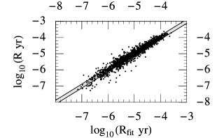
Figure 2.— This plot of the $\log_{10}$ of the Galactic rate versus our fit to the rate, shown for BH-BH, BH-NS, and NS-NS sample points (all superimposed). The shaded region is offset by a factor $1\pm 1/\sqrt{10}$. This region estimates the error expected due to random fluctuations in the number of binary merger events seen in a given sample. (See the appendix for a discussion of the number of sample points actually present in various runs.)

Figure 3.— A plot of the a priori probability distribution for the BH-BH (left), BH-NS (center), and NS-NS (right) merger rates, versus the $\log_{10}$ of the rate. These distributions were generated from the population synthesis code (dashed line) and fits (solid lines) assuming all parameters in the population synthesis code were chosen at random in the allowed region.

4. Constraints from NS-NS observations

In Sec. 2 we constructed two straightforward empirical constraints (i.e., confidence intervals for the formation rate of “visible” merging and wide NS-NS binaries) we could place on the output of population synthesis calculations. In this section, we apply these two constraints, individually and together, and determine their effect on rate predictions of population synthesis calculations.

Bounding merging NS-NS rate: Figure 4 superimposes the observational bounds taken from the observed merging NS-NS distribution (i.e., the 95% confidence interval; see Fig. 1) on top of the distribution of “visible” NS-NS merger rates obtained from unconstrained population synthesis. We limit attention only to those population synthesis models consistent with our constraint; specifically, we randomly choose population synthesis models, evaluate the “visible” merging NS-NS rate using our fit, and retain the model only if the rate lies within these two bounds. We find we reject 72% of models we initially considered plausible. For each of the small residual of consistent models, we can evaluate the BH-BH, BH-NS, and NS-NS merger rates (again using our fits). We find the merger rates increase slightly on average: the mean merger rate increases by a factor $\times 1.2$ for BH-BH, $\times 2$ for BH-NS, and $\times 2.2$ for NS-NS.

Figure 4.— A plot of the a priori probability distributions for the visible merging (top) and visible wide (bottom) NS-NS formation rates produced from population synthesis. The dashed curves denote the direct result from population synthesis; the solid curves denotes the result deduced from artificial data generated from a multidimensional fit to the visible wide and merging NS-NS rate data. The vertical lines are the respective 95% CI bounds presented in Fig. 1.

Bounding wide NS-NS rate: Figure 4 also shows the 95% confidence interval for the wide visible NS-NS formation rate (Fig. 1) on top of our a priori population synthesis distribution for the wide visible NS-NS formation rate. We find that with this constraint we have to exclude 80% of a priori plausible models. Using only models which satisfy this second constraint, we find DCO merger rates have dropped relative to our a priori predictions: the average BH-BH, BH-NS, and NS-NS merger rates are reduced by a factor $0.65$, $0.26$, and $0.22$, respectively.

Both constraints simultaneously: Very few population synthesis models (less than $2\%$) satisfy both constraints simultaneously. Since the set of consistent models is much smaller than initially permitted a priori, we have less uncertainty in our predictions: the standard deviation in the log of the merger rates has changed from our initial a priori uncertainty of 0.60, 0.55, and 0.63 (i.e., plus or minus a factor of 4, 3.5, and 4.3) for BH-BH, NS-NS, and BH-NS mergers, respectively, to 0.61, 0.44, and 0.48 (i.e., plus or minus a factor of 4, 2.8, and 3). Further, since the wide constraint proves slightly more restrictive, the mean merger rates have dropped slightly from our prior expectations: the average predicted merger rates are 1.1/Myr [BH-BH] (down by a factor $0.43$), 1.4/Myr [BH-NS] (down by a factor $0.24$), and 6.7/Myr [NS-NS] (down by a factor $0.25$).

Figure 5.— A plot of the a priori probability distribution for the BH-BH (top), BH-NS (center), and NS-NS (bottom) merger rates per milky way equivalent galaxy. As in Fig. 3, the dashed curves show the results obtained from our population synthesis calculations (i.e., our raw code results, smoothed); the thick solid curves show the results after we impose both our observational constraints (i.e., consistency with the observed number of visible wide and visible merging NS-NS binaries).

4.1. Advanced LIGO detection rates

While we have presented the number of mergers occurring per Milky Way equivalent galaxy, advanced LIGO’s inspiral detection range depends on the masses of the component objects. Specifically, one 4 km advanced LIGO detector (see Harry 2005) is expected to detect a binary with chirp mass ${\cal M}_{c}=(m_{1}m_{2})^{3/5}/(m_{1}+m_{2})^{1/5}$ (at signal-to-noise ratio 8) out to a distance

$$d=191\,{\rm Mpc}\;\left({\cal M}_{c}/1.2M_{\odot}\right)^{5/6}.$$ (8)

Thus, if the real merger rate and chirp mass distribution for type $\alpha$ are ${\cal R}_{\alpha}$ and $p_{\alpha}({\cal M}_{c})$, respectively, then LIGO will on average detect $\alpha$ merger events at a rate

$${\cal R}_{\alpha,\rm LIGO}=0.042\;{\cal R}_{\alpha}\left<({\cal M}_{c}/M_{\odot})^{15/6}\right>_{\alpha}$$ (9)

where $\left<({\cal M}_{c})^{15/6}\right>_{\alpha}=\int d{\cal M}_{c}p_{\alpha}({\cal M}_{c}){\cal M}_{c}^{15/6}$, and where for simplicity we assume a uniform distribution of Milky Way equivalent galaxies with density $0.01$/(Mpc)³ (see Nutzman et al. (2004) for a discussion of short-scale corrections to this distribution in the case of short-range interferometers, like initial LIGO).

Since Fig. 5 was produced using merger rate fits, we do not have the chirp mass information needed to translate that figure into a corresponding distribution for the LIGO detection rate. In what follows we adopt mean chirp masses as derived from all our models in the archives. We find:

$$\left<({\cal M}_{c})^{15/6}\right>_{\rm BH-BH}=111M_{\odot}^{15/6}$$ (10)

$$\left<({\cal M}_{c})^{15/6}\right>_{\rm BH-NS}=5.8M_{\odot}^{15/6}$$ (11)

$$\left<({\cal M}_{c})^{15/6}\right>_{\rm NS-NS}=2M_{\odot}^{15/6}.$$ (12)

These are to be compared to $224M_{\odot}^{15/6}$ for two $10$ M_⊙ BH, to $15.5M_{\odot}^{15/6}$ for a $10$ M_⊙ BH and a $1.4$ M_⊙ NS, and to $1.2M_{\odot}$ for two $1.4$ M_⊙ NS. Figure 6 presents our preliminary estimates for the advanced LIGO detection rate distribution. Note this figure provides the same information as Figure 5, except that the merger rates for each species have been rescaled according to Eq. (9).

Figure 6.— This plot shows our expectations for LIGO’s detection rates for merging BH-BH (solid line), BH-NS (dashed line), and NS-NS (dotted line) binaries. This plot was obtained directly from Fig. 5 using Eq. (9).

5. Summary and conclusions

In the context of matching theory with observations of the binary NS population, we have described how to constrain the predictions for DCO merger rates population synthesis codes such as StarTrack by using two specific observational constraints. We find that to be consistent with the rate statistics of the observed NS-NS population (at the 95% confidence interval), we must exclude at least 98% of all the models we think a priori likely. We do not focus on explicitly describing the seven-dimensional region of StarTrack model parameters consistent with our constraints, both because (i) we lack a compact way to describe a seven-dimensional region, and (ii) our region has meaning specifically for the StarTrack code. Other codes have different parameterizations of the same physical phenomena, leading to potentially quite different representations of the same constraint region. However, in Appendix C we give some information about the mean constraints on population synthesis parameters but also the strong variance around these mean values. As described in Section 4 and particularly via Fig. 5, to extract a physically meaningful statement about the effect of imposing constraints (as opposed to a describing information about parameters of one particular code), we have described how these constraints have improved our understanding of three DCO merger rates [BH-BH, BH-NS, and NS-NS]. We find that, using these two initial constraints, (i) the most probable merger rates (i.e., at peak probability density) are systematically lower than we would expect a priori, at least by a factor 2; and (ii) we reduce the uncertainty in the BH-NS and NS-NS merger rates by moderate factors (i.e., the standard deviation of $\log{\cal R}$ drops by 0.03 and 0.16, respectively).

This paper only outlines the beginning of a large program we have undertaken to better constrain our understanding of the evolution of single and binary stars and the associated predictions for gravitational-wave sources. We intend to add a few additional empirical constraints of DCOs (e.g., WD-NS binaries) and the lack of observations of certain binary compact objects (notably, BH-NS binaries). Apart from rate constraints, the observed properties of DCOs (mass ratios, orbital separations and eccentricities) could also be used as constraints. Further constraints (such as observations of pulsar kicks, which constrain the supernova kick distribution) can be added by other means, as prior distributions on the space of model parameters. We fully expect to have much stronger constraints on our understanding of population synthesis in the near future.

Stronger constraints, however, will require a considerably more systematic approach than the straightforward presentation we have used here. As the expected uncertainties decrease, greater care must be taken to include every uncertainty, no matter how minor, many of which for clarity we have neglected. For example, in future calculations we expect to include uncertainties in $L_{min}$ and $p$, our fit and rate estimates, and even the star formation rate we use to convert simulation results into rate estimates. Additionally, we will self-consistently choose the constraint confidence intervals in order to construct a meaningful posterior confidence interval on each merger rate.

Note on BH-pulsar rates: Recently, Pfahl et al. (2005) have estimated that BH-millisecond pulsar systems should be exceedingly rare: they find an upper bound of $10^{-7}$/year on the formation rate of binary systems containing a BH and a recycled pulsar. In our own computations, we have never seen such a system form, even though we have seen $\approx 6\times 10^{4}$ merging NS-NS binaries form. This result suggests the branching ratio for BH-PSR:NS-NS formation is $\ll 10^{-4}$. If we use a conservative value for the merging NS-NS formation rate, $10^{-4}/{\rm yr}/{\rm galaxy}$, then we expect the formation rate of BH-PSR binaries to be significantly less than $10^{-8}$/yr/galaxy, entirely consistent with their constraint.

Appendix A A. Calculating DCO event rates with population synthesis

This paper relies upon formation rates extracted from a large sequence of archived population synthesis calculations. This appendix describes how these archives were generated and used to produce formation rates. It also explains the expected uncertainties in each merger rate estimate.

A.1. How rates were estimated

Principles of archive generation: For a given combination of population synthesis parameters, we generate a large collection $N$ of binaries. To add a binary to the archive, we first generate progenitor binary parameters ($m_{1},m_{2},a,e$) [i.e., the two progenitor masses ($m_{1,2}$) and the initial semimajor axis ($a$) and eccentricity ($e$)] which are (i) drawn from the distribution functions presented in OKB and which (ii) satisfy any conditions we impose to reject binaries irrelevant to the study at hand – e.g., $m_{1,2}>4$, or more elaborate conditions described in OKB. (The latter conditions offer a significant speed improvement, but rely upon the experience gained in previous runs to insure that the conditions imposed do not reject physically relevant systems.) Given satisfactory initial conditions, binaries are assigned a randomly-chosen formation time, then evolved from whenever they form until the present day. Binaries are successively added to the archive until some termination condition is reached – typically, that the number $n$ of a given class of binaries, such as merging NS-NS binaries, has crossed a threshold (i.e., $n=10$).

Archive classes: Our population synthesis runs are summarized in Table 2. Each run of the population synthesis code falls into a certain class, depending on what choices were made for (i) the target systems on which the termination threshold was set (i.e., stop when we get $n$ merging BH-BH binaries; see column 2 of Table 2), (ii) the specific threshold $n$ chosen (i.e., which insures that the formation rate of the target system type is determined to an accuracy roughly $\sim 1/\sqrt{n}$; see column 3 of Table 2), and (iii) the combination of conditions applied to filter progenitor binary systems (see the last column of Table 2). In Table 2, the filters B, and S correspond to using the partitions presented in listed in Table 2 of OKB for BH-BH binaries (B) and NS-NS binaries (S); the ’W’ filter uses only the first NS-NS partition listed in Table 2 of OKB, which filters out WD progenitors. Note the first column of Table 2 merely provides a label for the archive class.

Applying archives: ¿From the ratio of the number of binaries of a given type seen to the number of binaries in a run, modulo a normalization factor presented in OKB, we can calculate the formation rates for any binary type of interest. However, to avoid extreme biases associated with a poor choice of filter or stopping condition, we use only certain archives to estimate merger rates, as described in Table 3. [In this table, all rates are total merger rates, with the exception of the last two rows, which correspond to the visible merging (v) and visible wide (vw) NS-NS binaries.]

Table 2Classes of runs

Type	Target	Number of runs	n	Filters
a	NS-NS	488	10	(none)
a’	NS-NS	137	100	S
a”	NS-NS	408	300	W
b	BH-BH	306	10	B
b’	BH-BH	285	10	W
c	BH-NS	357	10	W

Table 3Classes used for specific rates

Type	a	a’	a”	b	b’	c
BH-BH				x
BH-NS			x		x	x
NS-NS		x	x		x	x
NS-NS(v)	x	x	x		x	x
NS-NS(vw)		x	x		x	x

A.2. Understanding errors in rate estimates

Tables 2 and 3 provide the information needed to understand errors in our formation rate estimates.

Example: The BH-BH formation rate estimate is produced from a single archive ($b$). Archive $b$ is a collection of runs which stop when 10 merging BH-BH binaries are found; while the filters in this archive can prevent the formation of binaries involving NS, they do not significantly limit BH-BH binary formation. Therefore, archive $b$ is ideally suited to estimate the BH-BH merger rate to an accuracy of order $1/\sqrt{10}\approx 30\%$.

Example: The NS-NS formation rate estimate is produced from an amalgam of archives ($a^{\prime}$, $a^{\prime\prime}$, $b^{\prime}$, and $c$). None of these archives applies filters which prevent NS-NS formation, though one ($a^{\prime}$) applies filters which prevent the formation of nearly anything else. However, these archives do involve different termination criteria: the first two terminate when a large number of NS-NS binaries have formed, whereas the last two terminate when only 10 BH-BH or BH-NS archives have formed. If only the first two were used, we could guarantee the NS-NS merger rate to be known to within $10\%$ accuracy. However, to augment our statistics, we additionally included binaries from $b^{\prime}$ and $c$; while these archives should usually have many NS-NS binaries (cf. Fig. 3), we cannot guarantee any minimum number a priori. To simplify error estimates, we selected only those elements of $b^{\prime}$ and $c$ with more than $30$ merging NS-NS binaries. Thus, we expect our NS-NS rate to be known to within $20\%$ accuracy.

Example: The estimate for the visible wide NS-NS formation rate is the least accurate and most challenging calculation we performed. Since visible wide NS-NS systems were rare and since we did not (unlike the BH-BH case) have a simulation dedicated to discovering them, we had to scavenge through all the archives which could have produced them (i.e., not $b$) in sufficient numbers (i.e., not $a$) to permit a moderately accurate rate estimate. In practice, we selected those runs which formed more than $8$ wide visible NS-NS binaries, which should in principle give us an accuracy of order (few)$\times 35\%$. [In practice, we found a roughly 75% accuracy, comparable to the 65% accuracy of our next-most-accurate estimate (the BH-NS rate).]

Appendix B B. Sample fits to merger rates

This paper and in OKB rely upon fits to 7-dimensional functions obtained from the StarTrack population synthesis code. In this section, we provide an example of an explicit formula for a quadratic-order polynomial fit to the BH-BH merger rate. We express this fit in terms of the following dimensionless parameters $x_{k}\in[0,1]$: $x_{1}=r/3$ where $r\in[0,3]$ is a negative power-law index describing the mass ratio distribution assumed for binaries; $x_{2}=w$ characterizes the strength of stellar winds; the kick velocity distribution consists of two Maxwellian distributions with 1-D dispersions of $\sigma_{1}$ and $\sigma_{2}$, which are varied within [0,200 km s^-1] and (200, 1000 km s^-1], respectively, using two parameters: $x_{3}=\sigma_{1}/(200\,\text{km/s})$ and $x_{4}=-1/4+\sigma_{2}/800\,\text{km/s})$; a third parameter $x_{5}=s$ is used as the relative weight between low and high kick magnitudes; $x_{6}=\alpha\lambda$ is the effective common-envelope efficiency; and $x_{7}=f_{a}$ is the fraction of mass accreted by the accretor in phases of non-conservative mass transfer. [These parameters are discussed more thoroughly in OKB and in the original StarTrack paper Belczynski et al. (2002).] In terms of these parameters, we find the following quadratic fit to the BH-BH merger rate:

$$\log_{10}\left[{\cal R}_{\rm BH-BH}{\rm yr}\right] = -5.84517+1.30448\,{x_{1}}-0.406066\,{{x_{1}}}^{2}$$ (B1)

$$-0.310686\,{x_{2}}-0.407175\,{x_{1}}\,{x_{2}}+0.0142072\,{{x_{2}}}^{2}$$

$$+0.717803\,{x_{3}}-0.367487\,{x_{1}}\,{x_{3}}-0.48743\,{x_{2}}\,{x_{3}}$$

$$+0.29931\,{{x_{3}}}^{2}-0.770174\,{x_{4}}+0.242792\,{x_{1}}\,{x_{4}}$$

$$-0.0811259\,{x_{2}}\,{x_{4}}-0.0954582\,{x_{3}}\,{x_{4}}+0.113668\,{{x_{4}}}^{2}$$

$$+0.460929\,{x_{5}}-0.114934\,{x_{1}}\,{x_{5}}+0.490873\,{x_{2}}\,{x_{5}}$$

$$-0.691954\,{x_{3}}\,{x_{5}}+0.588787\,{x_{4}}\,{x_{5}}-0.810968\,{{x_{5}}}^{2}$$

$$-3.27367\,{x_{6}}-0.214978\,{x_{1}}\,{x_{6}}+0.674502\,{x_{2}}\,{x_{6}}$$

$$-0.779896\,{x_{3}}\,{x_{6}}+0.0891919\,{x_{4}}\,{x_{6}}+1.37719\,{x_{5}}\,{x_{6}}$$

$$+2.30296\,{{x_{6}}}^{2}+1.68227\,{x_{7}}-0.289592\,{x_{1}}\,{x_{7}}$$

$$-0.19047\,{x_{2}}\,{x_{7}}-1.18196\,{x_{3}}\,{x_{7}}-0.0281177\,{x_{4}}\,{x_{7}}$$

$$+0.517042\,{x_{5}}\,{x_{7}}+0.67596\,{x_{6}}\,{x_{7}}-0.454039\,{{x_{7}}}^{2}$$

Relation of this fit to those used in paper: The fit presented above is substantially less accurate than those actually used in our paper or in OKB: it is accurate only to within a factor $1.8^{\pm 1}$ (i.e., when we evaluate this fit at all of our trial points, we find the standard deviation between our results and the fit to be $\left<(\log{\cal R}_{BH-BH,fit}-\log{\cal R}_{BH-BH})^{2}\right>^{1/2}=0.26$). The fits actually used in this paper are typically cubic (120 parameters) and quartic (330 parameters) order. Given the large number of these parameters we chose to just provide the quadratic-order fit as an example above. However, the authors are happy to provide the much longer expressions for the higher-order fits used upon request by any reader.

The rate functions are demonstrably not separable: we cannot fit the rate functions well with a function of form $X_{1}(x_{1})X_{2}(x_{2})\ldots X_{7}(x_{7})$. Even this toy fit contains strong off-diagonal terms.

Appendix C C. Characterizing the consistent region of population synthesis models

Using our monte-carlo method to select models compatible with our constraints, we have found a relatively small seven-dimensional volume consistent with observations that corresponds to about 2% of all the runs we performed. Unfortunately – with some exceptions – this volumetric constraint does not translate to easily-understood and strong constraints on the individual parameters $x_{k}$ (using the notation of Appendix B). On the one hand, because the dimension is high, weak constraints on each parameter can correspond to very strong volumetric constraints. On the other hand, as demonstrated in Figure 77, because the consistent region is extended through our high-dimensional model space in a inhomogeneous anisotropic fashion, wide ranges of values of each parameter are still allowed, even after applying the constraints.

To provide the reader with a global view of the parameter values associated with the models that turn out to be consistent with our constraints, in Figure 77 we show the cumulative distributions of the consistent model parameter values for each of the seven parameters.

Figure 7.— Cumulative probability distributions $P_{k}(X)$ defined so $P_{k}(X)$ is the fraction of all models consistent with both constraints with $x_{k}<X$. The left panel shows the distributions for the 3 kick-related parameters $x_{3},x_{4},x_{5}$; in this panel, the bottom (dashed) curve denotes $P_{3}$, the middle (solid) curve denotes $P_{4}$, and the top dotted curve denotes $P_{5}$. The right panel shows the distributions for $P_{1}$ (solid top line), $P_{2}$ (dashed), $P_{6}$ (dotted), and $P_{7}$ (solid, bottom curve).

It is evident that the full ranges of values ([0,1]) are covered by the model parameters $x_{k}$ for the set of models consistent with the constraints. However, certain qualitative conclusions can be drawn: about 80% of the consistent models have kick relative weights (parameter $x_{5}$) below 0.3; about 50% of the consistent models have mass-ratio power-law indices smaller (in absolute value) than 0.6 ($x_{1}<0.2$; fractions of mass lost from the binary during non-conservative mass transfer phases in the range 20%-60% are not favored.

Given the above, any simple attempt to describe the consistent region will necessarily be a crude approximation. Nonetheless, for completeness we attempt to characterize the extended consistent region through its mean values. The mean model consistent with our constraints is given by:

$$\bar{x}=(x_{1},x_{2},\ldots,x_{7})=(0.33,\;0.46,\;0.61,\;0.53,\;0.18,\;0.43,\;0.57)$$ (C1)

These mean values correspond to a model with: fairly flat mass ratio distribution (power-law of $\simeq-1$); moderate stellar winds (strengths reduced by factors of $\simeq 2$); moderate kicks drawn from Mawellians with $\sigma_{1}\simeq 120$ km s^-1, $\sigma_{2}\simeq 625$ km s^-1, and with relative weights of $\simeq 20$% (favoring $\sigma_{2}$ over $\sigma_{1}$); moderate values for an effective common-envelope efficiency ($\alpha\lambda\simeq 0.4$ including the central concentration parameter $\lambda$); and moderately non-conservative mass transfer phases ($\simeq 40$% of the mass is lost from the binary). It is very important though to keep in mind the broad ranges of these parameters shown in Figure 77.

References

- Arzoumanian et al. (1999) Arzoumanian Z., Cordes J.M., Wasserman I. 1999, ApJ, 520, 696
- Bailes et al. (2003) Bailes, M., Ord, S. M., Knight, H. S., & Hotan, A. W. 2003, ApJ 595, L49
- Belczynski et al. (2002) Belczynski, K., Kalogera, V., and Bulik, T.2002, ApJ, 572, 407
- Belczynski et al. (2005) Belczynski, K., Kalogera, V., Taam, R., Rasio, F., Zezas, A., Bulik, T., Maccarone, T. 2005, ApJ, to be submitted
- Bethe & Brown (1998) Bethe, H. A. & Brown, G. B. 1998 ApJ, 506, 780
- Blitz (1997) Blitz, L. 1997, in CO: Twenty-Five Years of Millimeter-Wave Spectroscopy, ed. W. B. Latter et al. (Dordrecht: Kluwer), 11
- Burgay et al. (2003) Burgay, M. et al. 2003, Nature, 426, 531
- Caparello (1999) Capperello et al. 1999, AA, 351, 459
- Corongiu et al. (2004) Corongiu et al., 2004, Mem. S.A.It. Suppl. Vol. 5, 188
- Cutler & Thorne (2002) Cutler C. & Thorne, K. S. 2002 gr-qc/0204090
- Edwards & Bailes (2001) Edwards, R. T. & Bailes, M. 2001, ApJ, 547, L37
- Faulkner et al. (2005) Faulkner et al., 2005, ApJ, 618, L119
- Harry et al. (2005) Harry, G. et al, presentation at March 2005 LSC meeting, LIGO-G050088-00-R. LIGO documents can be obtained at http://admdbsrv.ligo.caltech.edu/dcc/
- Hobbs et al. (2004) Hobbs et al., 2004, MNRAS, 353, 1311
- Kim et al. (2004b) Kim, C. et al. 2004, 2004, ApJ 616 1109
- Hulse and Taylor (1975) Hulse, R. A. & Taylor, J. H. 1975, ApJ, 195, L51
- Kalogera et al. (1998) Kalogera, V. & Webbink, R. F. 1998, ApJ, 493, 351
- Kalogera et al. (2001) Kalogera et al., 2001, ApJ 556, 340.
- Kalogera et al. (2004a) Kalogera et al., 2004 ApJ 601 L179.
- Kalogera et al. (2004b) Kalogera et al., 2004, ApJ, 614, L137. [Erratum to ApJ, 601, L179]
- Kalogera (2004) Kalogera, K., proceedings of the 14th Workshop on General Relativity and Gravitation, Kyoto, Japan.
- Kaspi et al. (2000) Kaspi et al. 2000, ApJ, 543, 321
- Kim et al. (2003) Kim, C., Kalogera, V., & Lorimer, D. R. 2003, ApJ, 584, 985
- Kim et al. (2004a) Kim, C. et al. 2004, in Radio Pulsars, eds. F. Rasio and I. Stairs, in press
- Lundgren et al. (1995) Lundgren, Zepka, &Cordes 1995, ApJ 456, 305.
- Lyne et al. (2004) Lyne et al., 2004, MNRAS, 312, 698
- Nice et al. (1996) Nice, Sayer, & Taylor, 1996, ApJ, 466, L87
- Nutzman et al. (2004) Nutzman, P. et al, 2004, ApJ, 612, 364.
- O’Shaughnessy et al. (2005) O’Shaughnessy, R., Kalogera, K., Belczynski, K., 2005, ApJ 620, 385
- Peters and Mathews (1963) Peters, P.C., and Mathews, J., 1963, Phys. Rev. 131, 435
- Peters (1964) Peters, P.C., 1964, Phys. Rev. 136, 1224
- Champion et al. (2004) Champion et al., 2004, MNRAS, 350, 61
- Pfahl et al. (2005) Pfahl, E., Podsiadlowski, P, and Rappaport, S., 2005 ApJ, in press. See also astro-ph/0502122
- Stairs et al. (2002) Stairs, I. H., Thorsett, S. E., Taylor, J. H., Wolszczan, A. 2002, ApJ, 581, 501
- Wex et al. (2001) Wex, Kalogera, & Kramer 2001, ApJ, 528, 401
- Willems et al. (2004) Willems, B., Kalogera, V., and Henninger, M., 2004, Ap J, 616, 414
- Wolszczan (1991) Wolszczan, A. 1991, Nature, 350, 688
- van kerkwijk & Kulkarni (1999) van Kerkwijk, M. H. & Kulkarni, S. R. 1999, ApJ 516, L25