Accounting for the anisoplanatic point spread function in deep wide-field adaptive optics images

In this paper we present the approach we have used to determine and account for the anisoplanatic point spread function (PSF) in deep adaptive optics (AO) images for the Survey of a Wide Area with NACO (SWAN) at the ESO VLT. The survey comprises adaptive optics observations in the $K_{\mathrm{s}}$ band totaling $\sim 30\,\mathrm{arcmin}^{2}$, assembled from 42 discrete fields centered on different bright stars suitable for AO guiding. We develop a parametric model of the PSF variations across the field of view in order to build an accurate model PSF for every galaxy detected in each of the fields. We show that this approach is particularly convenient, as it uses only easily available data and makes no uncertain assumptions about the stability of the isoplanatic angle during any given night. The model was tested using simulated galaxy profiles to check its performance in terms of recovering the correct morphological parameters; we find that the results are reliable up to $K_{\mathrm{s}}\sim 20.5$ ($K_{\mathrm{AB}}\sim 22.3$) in a typical SWAN field. Finally, the model obtained was used to derive the first results from five SWAN fields, and to obtain the AO morphology of 55 galaxies brighter than $K_{\mathrm{s}}=20$. These preliminary results demonstrate the unique power of AO observations to derive the details of faint galaxy morphologies and to study galaxy evolution.

1 Introduction

In recent years an increasing number of adaptive optics (AO) systems have become available, which are capable of obtaining near-infrared images at the diffraction limits of 8-meter class telescopes. The scientific potential of such instrumentation is evident, but careful analysis of the resulting data is necessary to take account of the effects introduced by the method and the limitations of wavefront sensing and correction. A key point in the detailed analysis of AO images is the determination of the point spread function (PSF) across the whole field of view. However, this task is made more difficult because the performance and correction of the AO system are strongly anisoplanatic, and depend on many parameters such as the brightness of the reference guide star and the structure (height, size-scale, velocity) of the often quickly changing atmospheric turbulence. As a result, the PSF produced by an AO system can change rapidly in both time and position on the frame. For natural guide star (NGS) wavefront sensing, an extragalactic science target will typically be offset from the guide star by $\Delta\theta\sim$ 10″–30″ at best. As a result, the on-axis PSF no longer provides a suitable reference model for the off-axis PSF at the position of the scientific target. Until the advent of multi-conjugate adaptive optics systems on 8-m class telescopes (e.g., Le Louarn et al. lelouarn (2002)) full correction over a wide (1–2′) field will not be possible, and even then there will still be some PSF variation across the field (e.g., Vérinaud et al. verinaud (2003)). Therefore, a simple and generally applicable technique to model the variations in the PSF across a given science field would be of benefit to all wide-field adaptive optics data.

In this paper we present the approach we have used to account for the anisoplanatic PSF in deep adaptive optics images for the Survey of a Wide Area with NACO (SWAN). In the following section SWAN will be briefly described and motivated. In Sect. 3 some different proposed methods for PSF reconstruction will be analyzed, while in Sect. 4 our method will be explained and discussed. Computer simulations were used to validate the model, and their results are shown in Sect. 5. The first application of the model to five of the deep science fields will be presented in Sect. 6, and our conclusions follow in Sect. 7.

2 SWAN

In order to make full use of the new generation of telescopes, it is necessary to overcome the blurring effects of the atmosphere through the use of AO systems. These can allow ground-based telescopes to operate at or near the diffraction limit in the near infrared ($\sim 0.06\arcsec$ in K-band for an 8 meters telescope), resulting in high angular resolution and a low background in each pixel. In principle, such capabilities should offer important benefits for studying how galaxies form and evolve in the early universe. In practice, however, reaping the expected rewards has proved difficult, due to the small number of extragalactic sources known lying at distances $\Delta\theta\la 30\arcsec$ from bright ($V\la 13$) stars suitable for AO guiding.

The prospects for AO cosmology will undoubtedly improve with the widespread adoption of laser guide star (LGS) systems, since these impose less stringent requirements on the brightness and nearness of stars used for tip-tilt correction. In the mean time, to overcome the current shortage of extragalactic AO targets for NGS wavefront sensing, we have undertaken a program to identify and characterize faint field galaxies lying close to bright, blue stars at high Galactic latitudes (see, e.g., Larkin et al. larkin99 (1999); Davies et al. davies01 (2001)). Our own 42 southern bright star fields were initially imaged at seeing-limited resolution in $K_{\mathrm{s}}$ with SOFI at the ESO New Technology Telescope (Baker et al. baker (2003)), were followed up with optical imaging (Davies et al. davies05 (2005)), and are now targets for VIMOS optical spectroscopy at the ESO Very Large Telescope (VLT).

Figure 1: Example of a SWAN field: SBSF 18. The circles are the extended objects detected by SExtractor (SExtractor stellarity index $\mathrm{SSI}<0.9$), while the squares are point sources ($\mathrm{SSI}\geq 0.9$). A ghost of the bright guide star is marked with a cross.

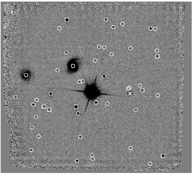
SWAN is the AO-assisted payoff of these seeing-limited preliminaries. Having already characterized large samples of objects in our bright star fields, we targeted them with NACO on the VLT in order to exploit the present generation of AO technology for galaxy evolution studies. NACO comprises the NAOS Shack-Hartmann AO module (Rousset et al. rousset (2003)) mated with the CONICA near-infrared camera (Lenzen et al. lenzen (1998)). Our choice of NACO observing mode was dictated by our desire to differentiate SWAN from previous HST/NICMOS surveys. First, we chose to prioritize survey area over depth, thereby improving SWAN’s sensitivity to rare objects and its robustness against cosmic variance. Second, we chose to image in $K_{\mathrm{s}}$, where NICMOS is less sensitive than in $J$ and $H$, thus making SWAN preferentially sensitive to red objects. Use of NACO’s $0.054\arcsec$ pixel scale (to maximize field of view) and the Strehl ratios of 30–60% typically achieved in $K_{\mathrm{s}}$ thus result in images that are undersampled. Each NACO pointing provides only a usable $\sim 0.75\,\mathrm{arcmin}^{2}$ of the full $55.5\arcsec\times 55.5\arcsec$ detector area, due to losses from dithering and the central star (see, e.g., Fig. 1). Nevertheless, the anticipated survey area that will result from assembling 42 such images will be – at $\sim 30\,\mathrm{arcmin}^{2}$ – some six times larger than the NICMOS survey of the HDF and flanking fields in $J$ and $H$ (Dickinson dickinson99 (1999), Dickinson et al. dickinson00 (2000)). In the ecology of near-IR surveys, SWAN aims to occupy a niche combining the high angular resolution of a space-based survey with the shallower depth and wider area of a ground-based survey, thereby probing sources that are compact, faint, red, and rare more effectively than any other survey to date. First results from an initial analysis of nine SWAN AO fields are presented in Baker et al. (baker05 (2005)), where NACO imaging is seen to detect a population of compact galaxies that cannot be identified as such in seeing-limited data.

To extract full information about the morphology of the sources detected in the SWAN images by taking into account the effects introduced by the PSF, it is necessary to develop a reliable model of the off-axis PSF in each of the fields. This task is not easy, however, as the AO PSF changes quickly in both time and position on the frame; in our case it is made even more difficult by the distinctive attributes of the SWAN observing strategy. First, because of their high Galactic latitudes, relatively few point sources are present in each of the fields, so that very few objects can be used as references to constrain how the PSF varies off-axis. In addition, in order to be background-limited so that the aim of the survey to detect faint galaxies can be realized, the on-axis star is always saturated on the science frames, meaning the on-axis PSF has to be obtained with separate unsaturated exposures. Finally, NACO has only very rarely been used to image stellar fields with the (undersampled) $0.054\arcsec$ pixel scale and the visible wavefront sensor; as a result, the VLT archive contains no suitable stellar fields that can help characterize the properties of the PSF as far off-axis as the SWAN images extend.

Given the above considerations, our data obviously pose several challenges for the recovery of intrinsic source parameters. Indeed, the same challenges will be faced by any extragalactic AO survey that relies on NGS or LGS wavefront sensing, and that efficiently builds up statistical samples of faint field galaxies by including a wide area around each bright star position. It is thus of general interest to devise a strategy to account for anisoplanaticism in deep, wide-field AO imaging.

3 Other proposed methods to quantify anisoplanaticism

There have been several methods proposed in the literature for estimating or calculating the off-axis PSF in an AO field. In this section we summarize these methods, and explain why they are not ideal for deep wide-field AO imaging with current instrumentation.

A theoretical analytical expression to model PSF variation and anisoplanaticism has been derived by Fusco et al. (fusco (2000)), who validated their method on both simulated and experimental data, leading to a reduction in the error on the magnitude estimation in stellar fields from more than 30% to only 1%. They showed that the total optical transfer function (OTF) is simply the product of the on-axis OTF with an anisoplanatic OTF. The on-axis OTF can be readily obtained, for example from real-time data accumulated by the AO system or a measurement of the on-axis PSF. The anisoplanatic OTF, however, requires an independent measurement of how the turbulence in the atmosphere depends on altitude, as quantified by the atmospheric refractive index structure constant $C^{2}_{n}$. In their example case this was obtained by balloon probes, but similar measurements are not usually available.

In a similar vein, the possibility of using AO measurements together with simultaneous scintillation detection and ranging (SCIDAR) measurements to reconstruct the $C^{2}_{n}$ profile and hence the off-axis PSF, was investigated by Weiß et al. (2002a ; 2002b ). While such measurements were made and analyzed, the idea was never brought to fruition and no such system has been installed as a permanent facility instrument.

An alternative semi-empirical approach was proposed by Steinbring et al. (steinbring (2002)), based on calibration images of dense stellar fields to determine the change in PSF with field position. Their results showed that this simple method reduces the error in the prediction of the FWHM of the PSF at large distances off-axis from 60% to only $\sim 20\%$. However, obtaining a suitable calibration field is not an easy task as atmospheric conditions can change rapidly. Steinbring et al. were able to complete the observations necessary to construct their mosaic images in less than 10 minutes. However, this approach is not practicable for even moderately deep-field observations. Our SWAN observations, for example, typically have integration time (without overheads) of 60 minutes. The additional time needed to switch continually between science and calibration fields would be prohibitive – even assuming that a suitable stellar field with a guide star of comparable brightness can be found not too far from the science field and also at a similar airmass. Furthermore, the authors point out that variations of up to 50% in the measured on-axis Strehl ratio ultimately limit the accuracy of the results.

A third approach to the problem was investigated by Tristram & Prieto (tristram (2005)). They parameterized the PSF using an elliptical Gaussian and a decaying elliptical exponential function. Starting with 11 parameters, they were able to eliminate all but four, which would need to be derived from stars in the science field. At high Galactic latitudes, the difficulty is that the number of point sources will be very limited in any science fields. To constrain 4 parameters reliably, the authors used 20 point sources, while our SWAN images always have fewer point sources per field – in a number of cases there are fewer than four – that are usually too faint for a detailed PSF fitting as is required here.

Given that it is not practical to apply any of these methods to SWAN or similar data, in the next Section we propose an alternative method suited to cases where there are very few unresolved sources in the science field (and those which do exist are often rather faint), and where one does not necessarily need a highly precise estimate of the PSF.

4 The PSF model for SWAN

To tackle the issue of anisoplanaticism in the SWAN data and to model an accurate PSF for every galaxy we detect we have developed a parametric model of the variations of the PSF across the field of view. This kind of approach is particularly convenient, as it uses only easily available data and makes no uncertain assumptions about the stability of the isoplanatic angle during any given night. Although the PSF reconstruction is not perfect, we will show that it is accurate enough for our purpose of measuring galaxy morphologies.

According to a theoretical analysis of the anisoplanatic effect in AO systems (e.g., Fusco et al. fusco (2000); Voitsekhovich & Bara v&b (1999)), the off-axis PSF can be expressed as a convolution between the on-axis PSF of the guide star with a spatially variable kernel, i.e.,

$$\textrm{PSF}(\textbf{{f}},\theta)=\textrm{PSF}(\textbf{{f}},0)\otimes\textrm{K}(\textbf{{f}},\theta)$$ (1)

Field	Date	Filter	Exp. Time	Strehl
			(min)	(%)
NGC 6809	15.12.02	$K_{\mathrm{s}}$	60	28
NGC 6752	06.09.03	$K_{\mathrm{s}}$	12	27

Table 1: Observations of PSF calibration fields. The Strehl ratio is that measured on-axis in the short exposure frames taken before and after the deep science exposures.

We will make the extreme assumption that the model of the kernel $\textrm{K}(\textbf{{f}},\alpha)$ is sufficiently well constrained that the difference in the kernel from one science field to the next is reduced to a single parameter, namely the isoplanatic angle. This is the most convenient solution for fields with sparse point source populations and, as we show, is able to reproduce a reasonable approximation to the PSF at any given location in the field of view using just the the on-axis PSF and a few reference point sources in the science field as calibration.

For each SWAN field the on-axis PSF was monitored by taking short unsaturated images of the bright star both before and after (and in some cases half-way through) the deep science exposure. These short exposure frames were taken in the $K_{\mathrm{s}}$ band, IB_2.21 ($\lambda_{c}=2.210\,\mathrm{\mu m}$, FWHM = 0.060 $\mu$m) or NB_2.17 ($\lambda_{c}=2.166\,\mathrm{\mu m}$, FWHM = 0.023 $\mu$m) filters. The integration time varied in the range 0.5–2.0 sec depending on the filter used. In addition, observations of galactic star cluster fields were planned periodically in order to build up a database of anisoplanatic PSFs. At the time of writing only two such calibration fields had been observed (see Table 1), but between them and the 7 SWAN fields with the highest numbers of point sources (see end of this section), included in Fig. 2, they still provide nearly 80 different point sources. These fields will be used in the following analysis as a test bench to derive a suitable parametric model for the off-axis PSF.

The images were reduced using PC-IRAF version 2.11.3. The presence of the bright star in the center of a field less than $1^{\prime}$ across made the data reduction a little more complex then usual, requiring two iterations of object masking and sky subtraction to avoid over-subtraction from very extended faint scattering around bright objects. For further details about data reduction see Cresci et al. (cresci (2005)).

Figure 2: Isoplanatic angle scaling. The Strehl ratios of point sources in the two calibration fields and 7 SWAN fields (SBSF 14, SBSF 15, SBSF 18, SBSF 24, SBSF 27, SBSF 28, SBSF 41) are plotted against their radial distance $\alpha$ from the AO guide star (in units of the corresponding isoplanatic angle). The black solid line is the theoretical curve used for fitting.

The isoplanatic angle of these fields was measured by considering – independently for each field – the Strehl ratio of the detected stars as a function of radius from the guide star. To these data we fit the theoretically expected function (e.g., Beckers beckers (1993); Roddier roddier (1999)):

$$\mathrm{SR}\propto\textrm{exp}\left[-\left(\frac{\Delta\theta}{\theta_{0}}\right)^{\frac{5}{3}}\right]$$ (2)

where $\Delta\theta$ is the offset angle from the guide star on the sky and $\theta_{0}$ the isoplanatic angle, defined as the separation angle at which the Strehl ratio has degraded by a factor $e$ with respect to the on-axis value. Although in a strict sense this refers to a telescope with infinite aperture (e.g., Beckers beckers (1993)), for our implementation this definition is adequate. A constant term was added to Eq. 2 in order to match the observed data. The resulting best fitting values for $\theta_{0}$ are 9.30″ and 6.61″ for NGC 6809 and NGC 6752 respectively. These are surprisingly small given the mean isoplanatic angle of the other seven SWAN fields of $\sim$17″. However, they do provide a larger range in $\theta_{0}$ over which our model can be constrained. The radial distances of all the point sources in the two calibration fields and in the 7 observed SWAN fields could then be normalized to their isoplanatic angles. This is shown in Fig. 2, where the Strehl ratios of the point sources in these fields are plotted against their rescaled separations from the AO guide star. It can be seen that all the points now lie on the same theoretical distribution, showing that the isoplanatic angle is the source of the principal variation between the different fields.

Figure 3: Upper panels: FWHM fits to the kernel. The radial (left panel) and tangential (right panel) FWHMs of the kernel to be convolved with the on-axis PSF to reproduce the observed PSF for the point sources in the calibration fields (diamonds) and in the seven SWAN fields of Fig. 2 (pluses), along with the best fitting second order polynomial. Lower panels: The total FWHMs of the observed point sources (radial at left, tangential at right) as a function of radial distance $\alpha$ from the guide star in units of the corresponding isoplanatic angle $\theta_{0}$, compared to the best fitting model for the kernel convolved with the guide star’s FWHM.

Our model is motivated by the fact that the wavefront error in the anisoplanatic kernel is dominated by the tip-tilt terms. This is borne out in practice, since the major degradation of the PSF observed in the calibration field images is an increasing radial elongation towards the guide star as one moves further off-axis. This suggests that, as a first approximation, one can represent the anisoplanatic kernel $\textrm{K}(\textbf{{f}},\alpha)$ with an elliptical Gaussian elongated towards the guide star. 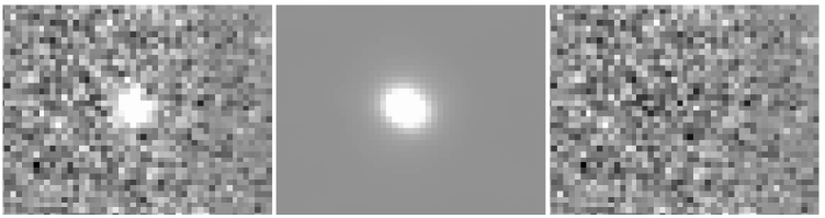For each of the point source in both of the calibration fields, we therefore derived the best fitting radial and tangential FWHMs of the elliptical Gaussian kernel to be convolved with the on-axis PSF in order to reproduce the observed off-axis PSF (see Fig. 3).
The fit was obtained by minimizing the sum of the squared difference between the observed star and models with different kernel FWHMs, weighted by the flux in each pixel of the star frame (in order to optimize the fit in the PSF core) and including all pixels brighter than 1% of the star peak. As the noise is dominated by the background, which is constant over each star, a noise term was not included in the expression, because it would have added just a constant scaling factor.

The residuals of the fitting are shown in Fig. 4 as a function of separation from the guide star. The residuals are defined as follows:

$$\textrm{Residuals}=\frac{\sqrt{\sum_{i}((\textrm{Star}_{i}-\textrm{Model}_{i})^{2}\cdot\textrm{Star}_{i})}}{\left(\sum_{i}(\textrm{Star}_{i})\right)^{1.5}}\cdot 100$$ (3)

where Star is extracted from the NACO data and Model is the best fitting kernel convolved with the on-axis PSF, so that the numerator is the quantity minimized during the fit, which was then normalized using the star brightness. It is clear that not all of the stars are equally well represented by the model, as expected due to the very simple kernel adopted to reproduce the PSF. However, the residuals do not depend strongly on the field in which the star lies (see Fig. 4) suggesting that the approach is robust to different conditions. The contribution of the noise to the residuals could be significant in the fainter point sources in the SWAN fields.

Figure 4: Residuals from the PSF fitting with the elliptical kernel for the point sources in the two calibration fields, NGC 6752 (triangles) and NGC 6809 (squares), and in the 7 SWAN fields of Fig. 2 (stars). The residuals plotted are defined in Eq. 3.

The FWHMs obtained along the radial and tangential directions were then fitted empirically as functions of the radial distance from the AO guide star. The function chosen was a second order polynomial, which was forced to a constant after reaching a maximum. Using higher order polynomials (or other analytical functions) just increased the number of free parameters without improving the fit. The final best fitting functions obtained are

for the radial axis:

$$\textrm{FWHM}_{r}(\arcsec)=\left\{\begin{array}[]{ll}0.107\cdot\alpha-0.00594\cdot\alpha^{2}&\textrm{if}\ \alpha\leq 9.1\\ 0.481&\textrm{if}\ \alpha>9.1\end{array}\right.$$ (4)

and for the tangential axis:

$$\textrm{FWHM}_{t}(\arcsec)=\left\{\begin{array}[]{ll}0.0871\cdot\alpha-0.00951\cdot\alpha^{2}&\textrm{if}\ \alpha\leq 4.6\\ 0.199&\textrm{if}\ \alpha>4.6\end{array}\right.$$ (5)

where $\alpha=\theta/\theta_{0}$ is the radial distance from the guide star rescaled using the isoplanatic angle. We notice that, although the method could be in principle applied to every AO system, the derived parameters were derived specifically for our SWAN dataset, and they have to be re-calibrated in order to use the same PSF model for any different adaptive optics system, instrument setting and operating conditions.
The variation of the total FWHM – i.e., the kernel convolved with the on-axis PSF – along both radial and tangential directions for the point sources in the calibration field is shown in the lower panels of Fig. 3. It can be seen how the total FWHM has a behavior consistent with what is observed for other AO PSFs (e.g., Flicker & Rigaut flicker (2002)).

Using the derived parametric model for the kernel, it is now possible to build the model PSF for any position in any of the SWAN fields with only an estimate of the isoplanatic angle in the respective field. The isoplanatic angle is derived by fitting the Strehl ratio of the few point sources detected in each science frame as a function of radius with Eq. 2. We have used SExtractor (Bertin & Arnouts bertin (1996)) to identify the sources in our SWAN NACO images, and as reference point sources for fitting the Strehl ratio, we use those with SExtractor stellarity index $\mathrm{SSI}\geq 0.9$ (see Fig.1). The derived isoplanatic angle is then used to rescale the radial distance from the guide star and to build the model PSF.

Figure 5: Comparison between the true and model PSFs for a point source in NGC 6752. The left panel shows the original star, the central panel the model for the corresponding position on the detector, and the right panel the residuals after subtracting the two. The star is located at 26.8″ from the AO guide star.

We additionally compared these results to those that could be obtained using PSFs generated by the PAOLA software (http://cfao.ucolick.org/software/paola.php), with an appropriate isoplanatic angle. PAOLA (Performance of Adaptive Optics for Large Apertures) is a set of functions and procedures written in IDL for calculating the performance of an AO system installed at the focus of an astronomical telescope. It relies on an analytic expression of the power spectrum of the corrected phase and its relation to the AO OTF. It therefore assumes that the AO system is “perfect”, failing to reproduce second order effects due to imperfections of the system. A set of PSFs were generated at different distances from the guide star, using in the model average parameters for the VLT and NACO. The radial distances of the PSFs were then rescaled to match the isoplanatic angle observed in the different fields. However, the match with the true PSFs was no better – and often worse – than that obtained with our parametric model, in particular worsening for increasing distances from the guide star.

Figure 6: The left panels show the RMS of the magnitude, Sérsic index and effective radius obtained from the GALFIT fits of the simulated profiles with Sérsic index $n=1$ as a function of the input magnitude. For each point, 100 galaxies with 10 different PSF were used (see text for details). The solid lines are the RMS obtained using the model PSF as an input for GALFIT, while the dashed ones are obtained with the original NACO PSF. The right panels show the results obtained for simulated profiles with Sérsic index $n=4$. In both cases it is clear that the parameters can be reliably recovered up to $K_{\mathrm{s}}\sim 20$.

5 Testing the PSF model with simulations of galaxy profiles

The PSF model developed in the previous section was carefully tested to see how well it performs in terms of recovering the correct morphological parameters of simulated galaxy profiles. The galaxy models were built by convolving a Sérsic (sersic (1968)) profile,

$$I(R)=I(R_{e})\times e^{\left(-b_{n}\times[(R/R_{e})^{1/n}-1]\right)}$$ (6)

(where $R_{e}$ is the effective radius, $n$ is the Sérsic index and $b_{n}$ is a constant that varies with $n$) with a true PSF extracted from either a calibration or a SWAN field. Our tests are particularly robust since we can compare the parameters recovered using the model PSF not only with those used as input for the simulations, but also with those recovered using the true PSF used to convolve the simulated profile. The primary aims of the simulations were to determine how well it was possible to estimate as a function of magnitude (1) the Sérsic index $n$ – and in particular whether it was possible to separate disk and elliptical profiles, and (2) the effective radius $R_{e}$ of the profile, which indicates the size scale of the galaxy.

We used Sérsic index $n=1$ for disk-like galaxies and $n=4$ for elliptical-like galaxies. For both types we ran several sets of simulations, each including 100 galaxies, at fixed magnitudes ranging from 17–22 mag in the $K_{\mathrm{s}}$ band, with the same pixel scale used in the SWAN images. The noise was set to the level expected for NACO integration time of 60 min for all the galaxies, since this is the typical integration time for a SWAN field. The inclination and position angle were random for each simulated profile, while the distribution of effective radii $R_{e}$ was chosen to roughly reproduce that observed in the real data – i.e. 40% of the objects having $R_{e}=0.1\arcsec$, 20% each with $R_{e}=0.2\arcsec$ and $R_{e}=0.3\arcsec$, and 10% each with $R_{e}=0.4\arcsec$ and $R_{e}=0.5\arcsec$. Ten different PSFs extracted from point sources in the calibration or SWAN fields were used for each set of 100 galaxies.

To recover the galaxy morphological parameters, we used GALFIT (Peng et al. peng (2002)), a widely used software package which fits an image of a galaxy and/or point source with one or more analytic functions. For our simulations we used GALFIT to fit a single Sérsic profile, leaving as free parameters the center of the galaxy, the Sérsic index $n$, the effective radius, the magnitude, the position angle and the axis ratio. The software needs an image of the PSF as input in order to fit the galaxy profile, both to deconvolve the original galaxy image and to convolve the derived model. For each simulated galaxy we ran GALFIT using both the true PSF from the NACO data – i.e., that which had been used to create the profile – and the corresponding model PSF, in order to compare the results.

The results of the simulations are shown in Fig. 6, where the uncertainties in the derived magnitude, Sérsic index, and effective radius are plotted as a function of magnitude for both disk-like and elliptical-like profiles. The results obtained using both the model PSF (solid lines) and true PSF (dashed lines) as input to GALFIT are shown, and it can be seen that these are in general very similar. Since using the true PSF is the best that can be done, we conclude that – in the application here of deriving the morphological parameters of galaxies – our model is a reasonable and valid approximation to the true PSF.

Figure 7: Disk/elliptical separation using GALFIT measurement of Sérsic index for simulated profiles with $K_{\mathrm{s}}=20$. The upper panel shows the input distributions of Sérsic index, while the central panel shows the results using the true NACO PSF used to build the profile as an input for GALFIT, and the lower panel what is obtained with the model PSF. The discriminating value for the Sérsic index $n=2$ (see text) is shown as a gray line.

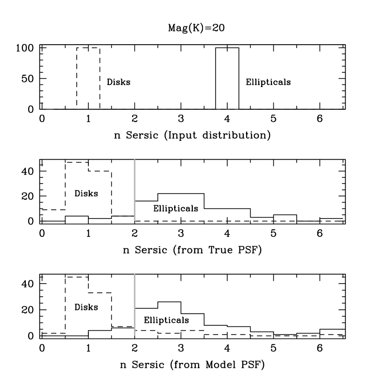
The most significant discrepancy between the two sets of results is a larger RMS in the Sérsic index for the simulated disk galaxies when the model PSF was used in GALFIT. In addition, the RMS for the Sérsic index is quite large ($\sim 1$) for elliptical galaxies, but this time for both the model and true PSFs. In principle this rather large uncertainty on the Sérsic index could restrict our ability to separate the two populations of disk-like and elliptical-like galaxies. However, in practice, the large variance for the ellipticals is due to a long tail to high values of $n$, as apparent in Fig. 7. We have found that starting with two populations of simulated galaxies with Sérsic index $n=1$ and $n=4$ respectively, only a small fraction (that increases with the magnitude of the galaxies, see Fig. 8) of disks was recovered with $n>2$, and few ellipticals were recovered with $n<2$. The two classes can be clearly distinguished up to $K_{\mathrm{s}}=20.5$, where 90% of the disks are recovered with Sérsic index $n<2$ and 90% of the ellipticals are recovered with Sérsic index $n>2$, using the model PSF in GALFIT (see Fig. 7). As a result, it is possible to set a threshold of $n=2$ that is able to discriminate between the two populations with a high degree of success. The fraction of disks recovered with a Sérsic index $n<2$ and the fraction of ellipticals recovered with $n>2$ are shown in Fig. 8 as a function of the magnitude, using both the model and true PSF. As the correct fitting of the Sérsic index is limited by the signal to noise of the sources, in order to correctly discriminate between disks and ellipticals at a fainter magnitude $K_{\mathrm{s}}$, the integration time should be scaled as $\Delta t\,(\mathrm{hr})=10^{[0.8\cdot(K_{\mathrm{s}}-20.5)]}$.

Figure 8: The fraction of ellipticals recovered with $n>2$ (left panel) and the fraction of disks recovered with a Sérsic index $n<2$ (right panel) as a function of the input magnitude. The dashed lines show the results obtained using the true NACO PSF, while the solid lines the ones obtained with the model PSF.

As an additional check of the usefulness of the model PSF, we repeated the experiment described above but giving GALFIT the observed on-axis PSF instead of either the model or true PSF. The outcome was that, even at relatively bright magnitudes $K_{\mathrm{s}}\simeq 17$, all the galaxies with a Sérsic index $n=4$ were actually recovered with an index of $n<2$, making it impossible to discriminate between the two populations. This emphasizes the important result of our simulations that it is only possible to discriminate between disk galaxies and elliptical galaxies using an anisoplanatic PSF, and that using our very simple PSF model is nearly as good as using the true PSF.

6 First results from five deep science fields

Prompted by the results on the simulated galaxy profiles, we have begun using our PSF model coupled with GALFIT to derive morphological parameters of the galaxies detected in a few of the SWAN survey fields in order to gain some insight into what we should expect, although clearly a full analysis requires the results of the dedicated redshift survey currently underway. In this paper we present the first results obtained from the first five fields, SBSF 14, SBSF 15, SBSF 18, SBSF 24 and SBSF 41, all of them already included in the preliminary discussion in Baker et al. (baker05 (2005)). The observations are summarized in Table 2, and the data were reduced using the same procedure adopted for the calibration fields (see Sect. 4).

Field	Date	Filter	Exp. Time	CE	$\theta_{0}$
			(min)	(%)	(″)
SBSF 14	15.12.02	$K_{\mathrm{s}}$	60	62	11.9
SBSF 15	17.12.02	$K_{\mathrm{s}}$	60	66	21.8
SBSF 18	17.12.02	$K_{\mathrm{s}}$	40	68	21.2
SBSF 24	21.03.03	$K_{\mathrm{s}}$	60	36	11.8
SBSF 41	14.06.03	$K_{\mathrm{s}}$	60	53	19.7

Table 2: Observations of the five SWAN fields included in the analysis here. CE is the encircled energy reported by the adaptive optics system in real time. The isoplanatic angle $\theta_{0}$ is that derived by the fit using point sources in the fields (see Sect. 4).

The performance obtained in these first SWAN fields compares favorably with that obtained by previous AO observations of faint field galaxies, e.g., Larkin et al. (larkin00 (2000)) and Glassman, Larkin, & Lafrenière (glassman (2002)). They obtained 12 $H$-band ($1.6\,\mathrm{\mu m}$) images of disk galaxies at $z\sim 0.5$ using the AO system on the Keck II telescope. They obtain FWHMs ranging from 0.050″ to 0.15″, and Strehl ratios of 1%–20%. Due to the very small field of view (4.5″) only one galaxy could be observed for each frame. The PSF was reconstructed using dedicated observations of faint off-axis stars with comparable offset, but different position angle, from the guide star. Due to the very low S/N obtained, the extraction of morphological parameters was run under several assumptions to limit the number of free parameters in the fit of a bulge and a disk to each galaxy. In addition, the AO galaxy profiles only had reasonable S/N out to 1″–2″ radius, thus limiting the constraints on the outer portions of the disks. Steinbring et al. (steinbring04 (2004)) imaged with the same AO system three galaxies selected because they had been observed previously with Hubble Space Telescope at optical wavelengths. However they conclude that higher S/N was needed in the AO images in order to match the HST data, and the results were limited due to poor constraints on the AO PSF.

Figure 9: Examples of single and multiple components fits by GALFIT of SWAN galaxies using the model PSF. In all images North is up and East is left. The distance of the galaxy from the guide star is shown in the upper right corner of each panel. For both galaxies, the $K_{\mathrm{s}}$ magnitude and the source identifier according to Baker et al. (baker (2003)) are reported. Upper panel: single component Sérsic fit ($K_{\mathrm{s}}=19.2$; $R_{e}=0.4\arcsec$; $n=0.6$; $b/a=0.6$; PA = 75). The left image is the original galaxy, the GALFIT best fitting profile is in the middle, and the residuals of the subtraction are on the right. Lower panel: comparison of the residuals between a single component fit (in the middle) and a two component fit (on the right), while the original galaxy is shown on the left. The final best fit was obtained with a disk component ($K_{\mathrm{s}}=19.6$; $R_{e}=0.4\arcsec$; $n=1.0$; $b/a=0.7$; PA = 76) and a point source ($K_{\mathrm{s}}=21.4$) in the center.

6.1 Source detection and modeling

In each SWAN field, sources were detected using SExtractor, with the appropriate parameters set to provide a positive detection for objects brighter than $1.5\,\sigma$ per pixel over an area of more then 3 pixels. To improve the detection of faint sources we used a Gaussian filter ($\sigma=1.5$ pixels) to smooth the image. False detections at the noisy borders of the mosaic and on the spikes and the ghost of the bright guide star were removed. For the former, a mask which indicted the fraction of the total integration time spent on each pixel was used; objects detected in pixels below a specified threshold were rejected. For the latter appropriate object masks were created. The resulting coverage of these 5 fields was $3.2\,\mathrm{arcmin}^{2}$, within which a total of 178 sources were detected down to a magnitude of $K_{\mathrm{s}}\sim 23$ ($K_{\mathrm{AB}}\sim 24.8$). Of these, 146 were allocated a stellarity index $\mathrm{SSI}<0.9$ by SExtractor, and hence classified as galaxies. The SExtractor classifications should be treated with caution since they assume a constant PSF across each field. However, all the objects classified as stars by SExtractor lie on an upper envelope in a Strehl versus radial distance plot, i.e., they have the highest Strehl ratio among the sources at the same distance from the guide star, supporting their classification as point sources.

We again used GALFIT to derive the morphological parameters of the detected galaxies. We used single component Sérsic profiles, providing the output from SExtractor as the initial guesses for magnitude, position, position angle, and axis ratio. For the deconvolution, a model PSF was created using the position of the center according to SExtractor and scaled according to the isoplanatic angle, which is shown for each field in Table 2. For each object, GALFIT was run twice, using as initial guesses for the second iteration the outputs of the first iteration.

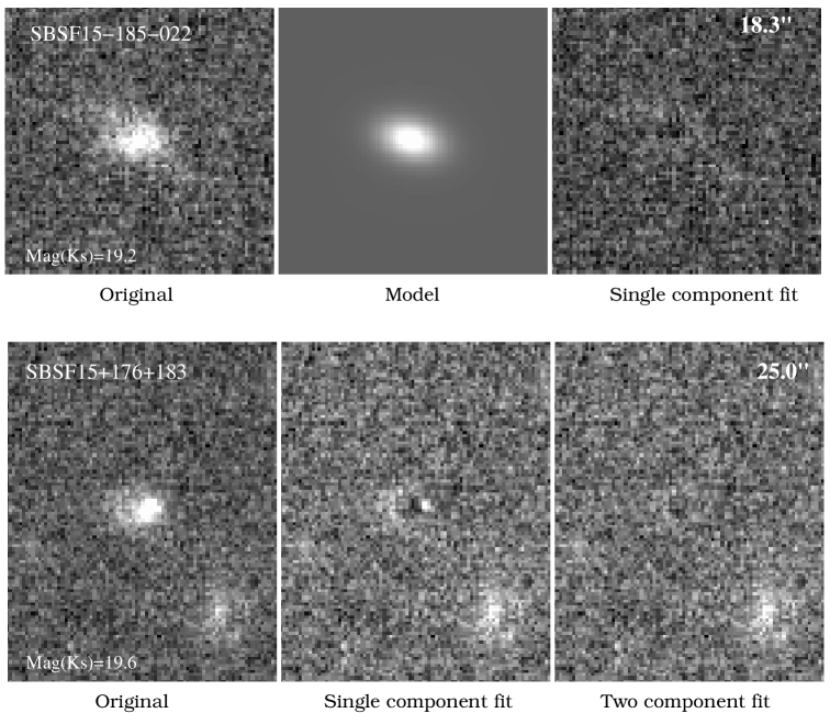
Some of the sources still showed bumps in the center or disk-like structures in the residuals after the single component fit. These objects were re-fitted using either two Sérsic components (bulge + disk) or a Sérsic component with an additional point source, to improve the fit and minimize the residuals.

A second iteration was also performed for close pairs or interacting galaxies; we fit both of them simultaneously to avoid incorrect background estimation or contamination from the companion. Some examples of single and multiple component fits are shown in Fig. 9. For galaxies fitted using multiple components, we report only the values for the larger scale component; the nuclear properties will be discussed elsewhere.

6.2 Source morphologies

The results obtained for the effective radii of the 55 galaxies brighter than $K_{\mathrm{s}}=20$ are shown in Fig. 10. While the redshifts of these objects are presently unknown, the magnitude-redshift relation of Cowie et al. (cowie (1996)) and the K20 survey (Cimatti et al. cimatti (2002)) indicate that at $K=20$ the median redshift is $z\sim 0.8-1$. At this redshift, our spatial resolution of $0.1\arcsec$, which also corresponds to the smallest effective radius bin, is equivalent to only 500 pc for typical cosmologies, hinting at the exciting potential of this work.

Using $n=2$ to discriminate between disks and ellipticals, we find there are 24 elliptical-like and 31 disk-like galaxies, with uncertainties below 10% on both numbers (see Section 5). In fact, with similar numbers of each type found, the number of ellipticals scattered into the disk-like category should roughly compensate the number of disks scattered out of it, and vice-versa.

Figure 10: Distribution of effective radii $R_{e}$ for the 55 sources detected down to $K_{\mathrm{s}}=20$ in the five SWAN fields observed with NACO (black hatched histograms), and for the 92 sources down to $K_{\mathrm{s}}=20$ observed in in larger fields centered on the same stars with SOFI (gray shaded histograms). The distribution is not corrected for completeness. For galaxies with more than one component, only the parameters of the larger scale (i.e., non-nuclear) one are used.

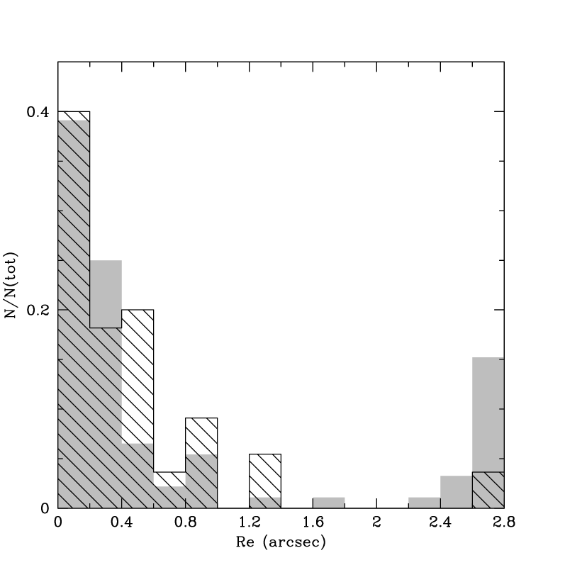
The distribution of effective radii is strongly peaked towards very compact sources, even down to scales of 0.1″. To check if this is due to a selection effect introduced by the AO correction – since adaptive optics data are inherently most sensitive to compact sources – we ran GALFIT on the same five fields, but using the seeing limited observations made with SOFI (Baker et al. baker (2003)). The same procedure was used, but a fixed PSF derived from the unsaturated guide star in each SOFI science fields was provided to GALFIT instead of the model PSFs. Not all the galaxies detected in the NACO images are present in the SOFI data, but on the other hand the SOFI spatial coverage is $\sim 5$ times larger, so that in the end we detected a comparable number of objects: 181 in total, 92 brighter than $K_{\mathrm{s}}=20$. The obtained distribution is shown in Fig. 10 as a gray histogram. The distribution of $R_{e}$ shows similar behavior in both AO and seeing limited data, suggesting that the observed distribution of $R_{e}$ in the SWAN fields is real and not due to selection effects. Nevertheless, the NACO distribution shows an excess of sources in the range $R_{e}=0.4-1.2$ with respect to SOFI, indicating that the better resolution of NACO is able to resolve many sources that in the SOFI data appear merely “compact” (e.g., a bright elliptical galaxy that NACO correctly recovers with $n=4$ and $R_{e}=1\arcsec$ is recovered by SOFI for a seeing of $0.7\arcsec$ as a compact source with $R_{e}=0.1\arcsec$, while a disky galaxy with $n=1$ and the same effective radius is correctly recovered by both).

Finally, the axis ratio distribution shows the co-sinusoidal distribution expected from random inclinations, except for a peak at $b/a=0$ due to very compact galaxies for which GALFIT could not calculate the axis ratio, and hence which were arbitrarily assigned to this bin.

6.3 Completeness

We have derived a first estimate of the completeness limit in our images using simulated galaxy profiles convolved with true NACO PSFs. This is a difficult task, as the completeness depends not only on the brightness and morphology of the source, but even on the distance from the guide star and the position on the frame. Therefore we derived a first estimate using only one reference PSF, a star at $21.2\arcsec$ from the guide star in SBSF 15. Fields with simulated galaxies of fixed magnitude and different $R_{e}$ (from $0.1\arcsec$ to $1.0\arcsec$) were created, and the sources were recovered using the same SExtractor parameters as used for the SWAN fields. We find that at $K_{\mathrm{s}}=20$ all the simulated elliptical-like galaxies were detected, while the disk-like galaxies were only 100% complete for effective radii smaller than $R_{e}=0.6\arcsec$. An average 50% completeness limit – i.e., the 50% limit for galaxies with $R_{e}=0.3\arcsec$ – is $K_{\mathrm{s}}\sim 21.5$ ($K_{\mathrm{AB}}\sim 23.3$) for disk-like galaxies and $K_{\mathrm{s}}\sim 23$ ($K_{\mathrm{AB}}\sim 24.8$) for elliptical-like ones. A more detailed analysis of completeness will be presented in a forthcoming paper (Cresci et al. cresci (2005)).

6.4 Confirming that we are accounting for anisoplanaticism

Figure 11: The difference $\Delta\phi$ between the radial vector from the guide star to the source at offset ($\Delta x,\Delta y$) and the source’s own major axis position angle $\phi$ as measured with SExtractor (left panel) with no PSF correction and with GALFIT (right panel) using the model PSF. In each panel the distribution for objects with angular distance from the guide star $<17\arcsec$ and $\geq 17\arcsec$ are shown (solid lines) as well as the total distribution of all sources (dashed line). Error bars are $\sqrt{N}$ for $N$ the number of objects in each bin.

The recovered position angle distribution can be used to indicate whether we are indeed correcting for the anisoplanatic PSF in an effective manner, and to evaluate possible biases in the results due to contributions by the wavefront correction that are still uncorrected by our PSF model. We have divided our sample in two subsets with separations $\Delta\theta<17\arcsec$ and $\Delta\theta\geq 17\arcsec$. This separation was chosen empirically as the approximate radius beyond which the PSF distortion becomes noticeable (see Baker et al. baker05 (2005)), but also corresponds to the average isoplanatic angle of the five fields in our analysis here. If no radial stretch due to PSF anisoplanaticism is present (or if this effect is fully taken into account by a PSF model) we would expect the distribution of $\Delta\phi=\phi-\arctan(\Delta x/\Delta y)$, i.e., the difference between the radial vector from the star to the source at offset ($\Delta x,\Delta y$) and the source’s own major axis position angle $\phi$, to be uniform over the interval $[-90^{\circ},+90^{\circ}]$ for both $\Delta\theta$ subsamples.

The distribution derived using SExtractor with no PSF anisoplanaticism correction (see Fig. 11, left panel) shows a clear peak at $\Delta\phi=0$ for objects at large radial distances from the guide star, i.e., these objects appear to be preferentially oriented towards the guide star. The right panel of Fig. 11 shows the same distribution as measured by GALFIT using the model PSF. As one would expect, in this case the peak is greatly reduced due to the model PSF. The small remaining overcounts could easily be due to random chance rather than a systematic effect. Indeed, analysis of this effect in the simulated galaxies indicates that it is completely removed.

7 Conclusions

In this paper we have presented a new approach to account for the PSF variations across the field of view in deep AO images, developed to correct the anisoplanaticism in SWAN images obtained with NACO at the ESO VLT, but also more generally applicable to other wide-field adaptive optics data. The survey is intended to overcome the current shortage of extragalactic AO targets and to study faint and compact field galaxies with unprecedented resolution in the near-IR. The observing strategy fully exploits the present capabilities of AO instrumentation, so that our method for PSF modeling may be broadly useful for AO cosmology.

We have described the PSF as the convolution between the on-axis PSF and a spatially varying kernel, an elliptical Gaussian elongated towards the AO guide star. We find that even adopting the most extreme case in which the the difference between the kernels in two different fields is given by a single parameter, namely the isoplanatic angle, the PSF can still be described with enough accuracy to extract reliable morphological parameters of field galaxies. This approach is particularly convenient, as it uses only easily available data and makes no uncertain assumptions about the stability of the isoplanatic angle during any given night. In addition, just a few point sources are required in each field to derive the isoplanatic angle and therefore compute the kernel.

Our simulations demonstrate that the model is able to recover reliably morphological parameters in a typical SWAN field with an integration time of one hour up to $K_{\mathrm{s}}\sim 20.5$ ($K_{\mathrm{AB}}\sim 22.3$), and that our very simple model is nearly as good as using the true PSF to account for anisoplanaticism.

Finally, we have presented the first morphological results for five SWAN fields, using the GALFIT package coupled with our model PSF. The recovered source parameters confirm that we are indeed accounting for anisoplanaticism, and show the unique power of AO observations to derive the details of morphology in faint galaxies. These results pave the way for the forthcoming analysis of all the obtained SWAN fields, which will combine for the first time the high angular resolution of a space-based survey with the shallower depth and wider area of a ground-based survey.