Regularized orbit models unveiling the stellar structure and dark matter halo of the Coma elliptical NGC 4807

Abstract

This is the second in a series of papers dedicated to unveil the mass structure and orbital content of a sample of flattened early-type galaxies in the Coma cluster. The ability of our orbit libraries to reconstruct internal stellar motions and the mass composition of a typical elliptical in the sample is investigated by means of Monte-Carlo simulations of isotropic rotator models. The simulations allow a determination of the optimal amount of regularization needed in the orbit superpositions. It is shown that under realistic observational conditions and with the appropriate regularization internal velocity moments can be reconstructed to an accuracy of $\approx 15$ per cent; the same accuracy can be achieved for the circular velocity and dark matter fraction. In contrast, the flattening of the halo remains unconstrained. Regularized orbit superpositions are applied to a first galaxy in our sample, NGC 4807, for which stellar kinematical observations extend to $3\,r_{\mathrm{eff}}$. The galaxy seems dark matter dominated outside $r>2\,r_{\mathrm{eff}}$. Logarithmic dark matter potentials are consistent with the data, as well as NFW-profiles (Navarro, Frenk & White 1996), mimicking logarithmic potentials over the observationally sampled radial range. In both cases, the derived stellar mass-to-light ratio $\Upsilon$ agrees well with independently obtained mass-to-light ratios from stellar population analysis. The achieved accuracy is $\Delta\Upsilon\approx 0.5$. Kinematically, NGC 4807 is characterized by mild radial anisotropy outside $r>0.5\,r_{\mathrm{eff}}$, becoming isotropic towards the center. Our orbit models hint at either a distinct stellar component or weak triaxiality in the outer parts of the galaxy.

1 Introduction

Interpreting the stellar kinematical data of ellipticals in terms of galaxy structural parameters requires knowing the gravitational potential as well as the distribution of stellar orbits, which – due to projection effects – is not directly given by observations. In equilibrium stellar systems, the phase-space distribution function (DF) describing the orbital state depends on phase-space coordinates only through the integrals of motion, admitted by the actual potential (Jeans theorem; e.g. Binney & Tremaine 1987).

In cases where integrals of motion can be expressed (or approximated) in terms of elementary functions, the DF can be parameterized explicitly. Several round as well as a couple of flattened ellipticals have been modelled based on this approach (e.g. Dehnen & Gerhard 1994; Carollo et al. 1995; Qian et al. 1995; Dejonghe et al. 1996; Gerhard et al. 1998; Emsellem, Dejonghe & Bacon 1999; Matthias & Gerhard 1999; Statler, Dejonghe & Smecker-Hane 1999; Kronawitter et al. 2000; Saglia et al. 2000; Gerhard et al. 2001). On the other hand, Schwarzschild’s (1979) orbit superposition modelling technique provides fully general dynamical models for any axisymmetric or triaxial potential and has been successfully applied to a growing number of early-type galaxies (e.g. Rix et al. 1997; Cretton & van den Bosch 1998; Cretton, Rix & de Zeeuw 2000; Gebhardt et al. 2000; Cappellari et al. 2002; Verolme et al. 2002; Gebhardt et al. 2003; Romanowsky et al. 2003; Copin, Cretton & Emsellem 2004; Valluri, Merritt & Emsellem 2004; Krajnović et al. 2005).

Even if the number of dynamical models is steadily increasing, the only comprehensive investigation of elliptical galaxy DFs addressing the question of dark matter in these systems is still the basis-function based spherical modeling of 21 round galaxies by Kronawitter et al. (2000) and Gerhard et al. (2001). To extend the results found there and in the handful of studies of individual objects quoted above, we started a project aimed to probe a sample of flattened early-type galaxies in the Coma cluster, collecting major (Mehlert et al., 2000) and minor axis (Wegner et al., 2002) kinematical data. The goal is to investigate the dynamical structure and dark matter content of these galaxies.

Most present-day orbit superpositions, conceptionally based on Schwarzschild’s original implementation, do not automatically provide the entire phase-space DF, but only orbital occupation numbers or weights, respectively, characterizing the total amount of light carried by each orbit. In principle, changing the orbit sampling strategy allows one to infer the DF from any orbit superposition (Häfner et al., 2000), but this approach has not yet been followed fully. To take advantage of both, the full generality of orbit superpositions and the availability of DFs, we extended the orbit superposition code of Richstone & Tremaine (1988) and Gebhardt et al. (2000) to reconstruct phase-space DFs in the axisymmetric case (Thomas et al., 2004).

Recovering stellar DFs from photometric and kinematic observations – in particular the application of non-parametric methods like orbit superpositions – invokes regularization in order to pick up smooth phase-space distributions (e.g. Richstone & Tremaine 1988; Merritt 1993). Different regularization schemes have been applied in the context of orbit libraries, among them variants of minimizing occupation number gradients in orbit space (Zhao, 1996) and maximum entropy (Richstone & Tremaine, 1988). The proper amount of regularization has thereby commonly been adjusted to the data (e.g. Rix et al. 1997; Verolme et al. 2002; Richstone et al., in preparation).

One aim of this paper is to readdress the question of how much regularization is needed to recover galaxy internal structural properties from observations with spatial sampling and noise typical for our sample of Coma galaxies. To this end we study observationally motivated reference models under realistic observational conditions and optimize regularization with respect to the reconstruction of intrinsic input-model properties (see e.g. Gerhard et al. 1998; Cretton et al. 1999). By simulating and recovering reference galaxies we also determine to which degree the internal mass structure and orbital content are constrained by observational data in our sample. Furthermore $\chi^{2}$-statistics are measured to assign confidence intervals to real galaxy orbit superpositions.

To demonstrate the prospects of regularized orbit superpositions for our project we also present an application to one galaxy. We have chosen the faint giant E2 elliptical NGC 4807 ($M_{B}=-20.76$ for $H_{0}=69\,\mathrm{km/s/Mpc}$ from Hyperleda) for the following reasons: (1) The galaxy has a prominent boxy photometric feature in the outer parts constraining its inclination. (2) Stellar kinematic data reach out to 3 $r_{\mathrm{eff}}$ along the major axis probing its dark halo outside the galaxy main-body. (3) NGC 4807 lacks significant minor-axis rotation and isophotal twist and thus is an ideal target for axisymmetric modelling. (4) The galaxy is only mildly flattened and the dynamical models can be compared with earlier studies of similar galaxies done mostly in the spherical approximation.

The paper is organized as follows. Sec. 2 summarizes the observations of NGC 4807, Sec. 3 outlines the orbit superposition technique. In Sec. 4 Monte-Carlo simulations performed to derive the optimal regularization are described and the achieved accuracy of galaxy reconstructions follows in Sec. 5. Orbit models for NGC 4807 are presented in Secs. 6-8. The paper is closed with a combined summary and discussion of the results in Sec. 9.

2 NGC 4807: model input

In the following we assume a distance $d=100\,\mathrm{Mpc}$ to NGC 4807 (corresponding to $H_{0}=69\,\mathrm{km/s/Mpc}$) and take $r_{\mathrm{eff}}=6.7$ arcsec as its effective radius (Mehlert et al., 2000).

2.1 Photometric data

The photometric data are combined from two different sources. For the outer parts of NGC 4807 Kron-Cousins $R_{C}$ band CCD photometry is drawn from Mehlert et al. (2000), consisting of profiles for the surface brightness $\mu_{R}$, ellipticity $\epsilon$ and isophotal shape parameters $a_{4}$ and $a_{6}$ out to $\approx 5.5\,r_{\mathrm{eff}}$ (see Bender & Möllenhoff 1987 for a definition of $a_{n}$). A seeing of 2 arcsec during the observations causes the profiles to be unresolved in their central parts (at $d=100\,\mathrm{Mpc}$ one arcsec corresponds to $0.485\,\mathrm{kpc}$). To increase the central resolution, the ground-based data are supplemented by corresponding profiles for $\mu_{V},\epsilon,a_{4}$ and $a_{6}$ extracted from archival HST V band data (Principal Investigator: John Lucey; Proposal ID: 5997).

The two surface brightness profiles $\mu_{R}$ and $\mu_{V}$ are joined by shifting the HST V band according to the average $\langle\mu_{R}-\mu_{V}\rangle$ taken over the region $0.75\,r_{\mathrm{eff}}\leq R\leq 3\,r_{\mathrm{eff}}$, where both data sets overlap and seeing effects are negligible. The shift $\langle\mu_{R}-\mu_{V}\rangle$ is well defined with a rms of only $0.015\,\mathrm{mag}$.

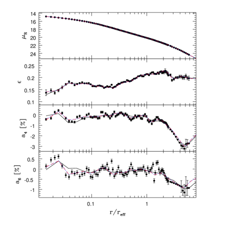
For the orbit models ground-based photometry is used outside $R\geq 3\,r_{\mathrm{eff}}$ and HST data inside $R<3\,r_{\mathrm{eff}}$. Fig. 1 shows the combined $\mu_{R}$, $\epsilon$, $a_{4}$ and $a_{6}$ profiles applied for the modelling.

2.2 Deprojection

Figure 1: Photometric data for NGC 4807 (dots with error bars, from top to bottom: surface brightness $\mu_{R}$, ellipticity $\epsilon$, isophotal shape parameters $a_{4}$ and $a_{6}$) and three deprojections: edge-on deprojection (solid); $i=50\degr$-deprojection (dashed); disky $i=50\degr$- deprojection (dotted).

In the implementation of Schwarzschild’s modelling technique used here, orbit models are not directly fitted to observed photometry. Instead, the deprojected luminosity density is used as a boundary condition for any orbit superposition (see Sec. 3.4).

Deprojection of axisymmetric galaxies is unique only for edge-on systems (inclination $i=90\degr$; Rybicki 1987). For any inclination $i<90\degr$ disk-like konus-densities can be added to the luminosity profile without affecting its projected appearance for any $i^{\prime}<i$ (Gerhard & Binney, 1996). From $i=90\degr$ to $i=0\degr$ the variety of different luminosity models projecting to the same galaxy image generally increases.

Deprojections for NGC 4807 are obtained with the program of Magorrian (1999). The code allows one to explore the full range of luminosity densities consistent with the photometric data by forcing the deprojection towards different internal shapes. For example, at any given inclination $i$ the goodness of fit of the deprojection can be penalized towards any degree of internal boxiness and diskiness, respectively. The deprojections are fitted without seeing-correction, since our joint photometry includes ground-based data only outside $R\geq 3\,r_{\mathrm{eff}}$, where seeing effects are negligible. Outside the last measured photometric data point ($R\geq 5.5\,r_{\mathrm{eff}}$), the photometry is extrapolated by a de Vaucouleurs profile fitted to the inner parts of the galaxy. The isophotes outside $R>5.5\,R_{\mathrm{eff}}$ are assumed to be perfect ellipses with a constant flattening corresponding to the galaxy’s outermost measured ellipticity.

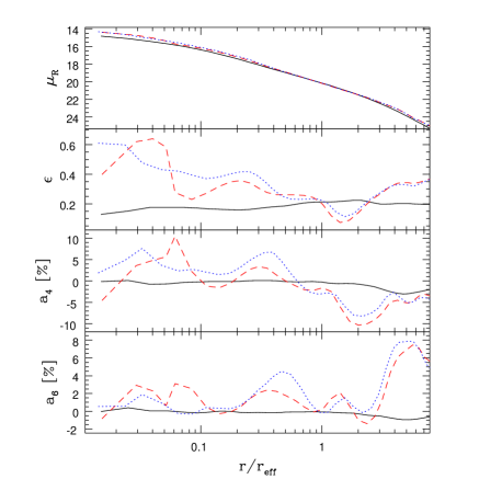
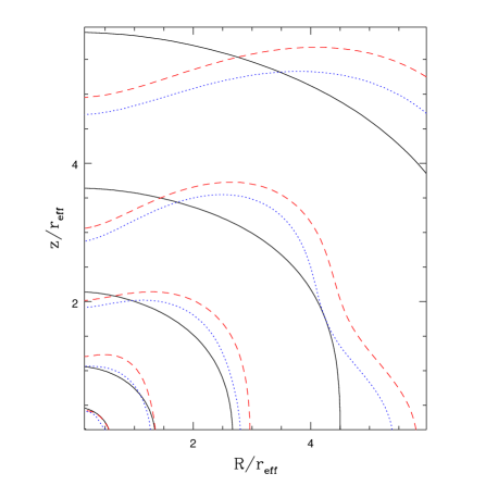
From the average flattening $\langle q\rangle=0.8$ of NGC 4807 we expect an inclination angle $i>38\degr$. Lower viewing angles would require density distributions intrinsically flatter than E7, which are not observed. In Fig. 1 three representative deprojections are overplotted to the photometric data: the (unique) $i=90\degr$-deprojection; a deprojection at $i=50\degr$ without any shape penalty; a disky $i=50\degr$-deprojection. All three luminosity models are equally consistent with the data. The differences between the models are illustrated in Fig. 2, which displays the isophotal shape parameters and the corresponding isophotes of the deprojections as they appear viewed from edge-on. At this viewing angle internal density distortions show up the strongest.

As Fig. 2 reveals, both deprojections at $i=50\degr$ are heavily boxy around $R\approx 2\,r_{\mathrm{eff}}$ ($a_{4}\approx-10$ per cent for the deprojection without shape preference and $a_{4}\approx-8$ per cent for the disky deprojection). These distortions are a reflection of the drop in $a_{4}$ at $R>3\,r_{\mathrm{eff}}$ in the data of NGC 4807. Projected density distortions progressively strengthen in deprojection from $i=90\degr$ to $i=0\degr$ and assuming $i=50\degr$ already causes a considerable amplification. Near the center – where the observed isophotes are consistent with being purely elliptical – the disky deprojection appears smoother with on average larger $a_{4}$, albeit lacking the strong $a_{4}$-peak occurring in the deprojection without shape preference at $R=0.05\,r_{\mathrm{eff}}$.

We have constructed orbit models for both, the $i=90\degr$ and the non-disky $i=50\degr$ deprojections, but the heavily distorted density distributions at $i=50\degr$ lead us to expect that we likely view NGC 4807 close to edge-on.

Figure 2: Projected appearance of the three deprojections shown in Fig. 1 when seen edge-on. The top panel shows isophotal shape parameters (cf. Fig. 1), the bottom panel displays the corresponding isophotes. Solid: $i=90\degr$ deprojection; dashed: $i=50\degr$-deprojection; dotted: disky $i=50\degr$-deprojection.

2.3 Kinematic data

The kinematic data are described in Mehlert et al. (2000) and Wegner et al. (2002). They consist of two long-slit spectra for the major and the minor axis, respectively. Profiles of lower order Gauss-Hermite coefficients $\gamma_{0}$, $v$, $\sigma$, $H_{3}$ and $H_{4}$ (Gerhard, 1993; van der Marel & Franx, 1993) parameterizing the line-of-sight velocity distribution (LOSVD) reach out to $3\,r_{\mathrm{eff}}$ along the major-axis and out to $0.6\,r_{\mathrm{eff}}$ along the minor-axis. Our orbit models are not directly fitted to the observed Gauss-Hermite parameters, but to binned LOSVDs. Therefore the Gauss-Hermite parameters are transformed into suitable LOSVDs as follows. First, the Gauss-Hermite series according to the observed $\gamma_{0}$, $v$, $\sigma$, $H_{3}$ and $H_{4}$ is evaluated at 1000 values of line-of-sight velocity $v_{\mathrm{los}}$, linearly spaced in the range $-4\,\sigma\leq v_{\mathrm{los}}\leq 4\,\sigma$. At each of the sampled projected velocities error bars $\Delta\mathrm{LOSVD}$ are assigned to the LOSVD from the errors in the corresponding Gauss-Hermite parameters by means of Monte-Carlo simulations. The LOSVD is then binned appropriately for comparison with the orbit library (see Sec. 3.1 below).

For NGC 4807, the scatter in kinematical data from different sides of the galaxy is mostly negligible compared with the statistical errors in the data. Therefore, the orbit models are fitted to a symmetrized data set, derived by averaging the Gauss-Hermite parameters from each side. The largest scatter appears in the outermost major-axis $H_{4}$-measurement. To infer the impact of its uncertainty on the reconstructed DF, we separately refitted the mass model that most closely matches the symmetrized data set, to the kinematics of the two different sides of NGC 4807. Both fits lead to similar models in terms of DF and internal kinematical structure, suggesting that the asymmetry in this single measurement does not largely affect our results.

3 Orbit superposition models

Our method of setting up orbit libraries to construct best fitting models is described in detail in Richstone et al. (in preparation) and in Thomas et al. (2004). Here, we only briefly outline some aspects of the method relevant to the present paper.

To recover the mass distribution of a given galaxy by orbit libraries, a grid of (parameterized) trial potentials is probed. In each trial potential (Sec. 3.2) a large set of orbits is calculated (Sec. 3.3) and an orbit superposition is constructed that best matches the observational constraints (Sec. 3.4). The best-fitting mass parameters with corresponding errors then follow from a $\chi^{2}$-analysis.

3.1 Basic grids

For comparison with observations the meridional plane of the orbit model as well as its projection onto the plane of the sky are divided into bins in radius $r$ and polar angle $\vartheta$. The grid in radius is logarithmic in the outer parts and becomes linear in the inner parts; the angular bins cover equal steps in $\sin\vartheta$ (see Richstone et al, in preparation, for details). For NGC 4807 the models are calculated in $N_{r}\times N_{\vartheta}=200$ bins with $N_{r}=20$ and $N_{\vartheta}=10$. Each spatial bin of the model’s sky-projection is subdivided into $N_{\mathrm{vel}}=15$ bins in projected velocity for the purpose of fitting the library to the observed kinematics.

3.2 Luminous and dark mass distributions

Luminous matter.

We assume that the luminous mass of NGC 4807 is sufficiently characterized by a constant stellar mass-to-light ratio $\Upsilon$ (see also Sec. 9 and Fig. 22 for a verification of this assumption). The stellar mass density then reads $\Upsilon\,\nu$, where the luminosity density $\nu$ is taken from the deprojections of Sec. 2.2.

Dark matter.

Modelling of spiral and dwarf galaxy rotation curves indicates shallow inner dark matter density distributions, i.e. logarithmic density slopes $\gamma\equiv\mathrm{d}\ln(\rho_{\mathrm{DM}})/\mathrm{d}\ln(r)\approx 0$ (e.g. de Blok et al. 2001; Gentile et al. 2004). Flat dark matter density cores also fit to the kinematics of round ellipticals (Gerhard et al., 2001), although Rix et al. (1997) found steeper profiles consistent with observations of NGC 2434. Some optical or radio rotation curves also allow density slopes up to $\gamma\leq-1$, but they do not prefer steep profiles (Swaters et al., 2003).

Shallow dark matter density profiles conflict with predictions of (pure dark matter) cosmological $N$-body simulations. In the $\Lambda$CDM scenario, dark matter distributions with central density cusps around $-1.5<\gamma<-1$ are found (e.g. Moore et al. 1999; Navarro et al. 2004). Similar steep profiles emerge in warm dark matter (Colin, Avila-Reese & Valenzuela 2000; Knebe et al. 2002), whereas self-interacting dark matter offers central $\gamma\approx 0$ (Davé et al., 2001).

To probe the whole diversity of theoretically and observationally motivated profiles we allow for two different dark matter distributions, one with central $\gamma=0$, representative of shallow profiles and another with central $\gamma=-1$, representative of the steeper cases.

Cored profiles.

A dark matter distribution that provides asymptotically flat circular velocity curves in combination with flat ($\gamma=0$) inner density cores is given by the logarithmic potential (Binney & Tremaine, 1987)

$$\Phi_{\mathrm{LOG}}(R,z)=\frac{v_{c}^{2}}{2}\ln\left(r_{c}^{2}+R^{2}+\frac{z^{2}}{q^{2}}\right),$$ (1)

where $R=r\cos(\vartheta)$, $z=r\sin(\vartheta)$ are cartesian coordinates in the meridional plane and $\vartheta=0\degr$ corresponds to the equator. The density distribution generating $\Phi_{\mathrm{LOG}}$ reads (Binney & Tremaine, 1987)

$$\rho_{\mathrm{LOG}}(R,z)\propto v_{c}^{2}\frac{(2q^{2}+1)r_{c}^{2}+R^{2}+2(1-\frac{1}{2q^{2}})z^{2}}{(r_{c}^{2}+R^{2}+z^{2}/q^{2})^{2}\;q^{2}}$$ (2)

and is positive everywhere for $q\in[1/\sqrt{2},1]$. The flattening of the density distribution (2) differs from that of the potential $q$. It is generally smaller and varies with radius. In the following, we will only consider cored profiles with $q=1.0$ (spherical). Together with the assumption of a constant mass-to-light ratio $\Upsilon$ models with dark matter distributions according to equation (2) can be seen as analogues to maximum-disk models of spiral galaxies and have been called maximum-stellar-mass models (Gerhard et al., 1998).

Cuspy profiles.

A representative cuspy mass distribution fitting simulated dark matter halos over a wide range of radii is the Navarro-Frenk-White (NFW) profile (Navarro, Frenk & White, 1996)

$$\rho_{\mathrm{NFW}}(r,r_{s},c)\propto\frac{\delta_{c}}{(r/r_{s})(1+r/r_{s})^{2}},$$ (3)

with a central logarithmic density slope $\gamma=-1$. The parameter $\delta_{c}$ in equation (3) is related to a concentration parameter $c$ via

$$\delta_{c}=\frac{200}{3}\frac{c^{3}}{\mathrm{ln}(1+c)-c/(1+c)}.$$ (4)

By the substitution $r\rightarrow r\sqrt{\cos^{2}(\vartheta)+\sin^{2}(\vartheta)/q^{2}}$ equation (3) provides halos with a constant flattening $q$.

In CDM cosmology the two parameters $c$ and $r_{s}$ turn out to be correlated in the sense that higher mass halos are less concentrated, with some scatter due to different mass assembly histories (Navarro, Frenk & White 1996; Jing & Suto 2000; Wechsler et al. 2002). The corresponding relation reads

$$r_{s}^{3}\propto 10^{(A-\log c)/B}\left(200\,\frac{4\pi}{3}\,c^{3}\right)^{-1}.$$ (5)

Here, we take $A=1.05$ and $B=0.15$ (Navarro, Frenk & White 1996; Rix et al. 1997), which – for the concentrations $5<c<25$ considered here – is equivalent to within 10 per cent to the relation given in Wechsler et al. (2002) for the now standard $\Lambda$CDM.

Total gravitating mass and potential.

Luminous and dark matter components combine to the total mass density

$$\rho=\Upsilon\,\nu+\rho_{\mathrm{DM}},$$ (6)

with $\rho_{\mathrm{DM}}$ being either $\rho_{\mathrm{LOG}}$ or $\rho_{\mathrm{NFW}}$. The potential $\Phi$ follows by integrating Poisson’s equation.

3.3 Orbit collection

Given $\Phi$, a large set of orbits is calculated in order to sample the phase-space of the potential. Energies $E$ and angular momenta $L_{z}$ of the orbits are chosen to connect every pair of equatorial radial grid bins by at least one equatorial orbit. The surfaces of section (SOS) connected to pairs of ($E,L_{z}$) – here the upward orbital crossings with the equator – are densely filled with orbits of all available shapes (Thomas et al., 2004). A typical orbit library contains between 6500 and 9500 orbits for $L_{z}>0$. Each orbit’s retrograde counterpart with $L_{z}<0$ is included in the library by reversing the azimuthal velocities appropriately. In total a typical library then contains between 13000 to 19000 orbits.

3.4 Orbit superposition

Any superposition of a library’s orbits generates a model with a specific internal density distribution and specific projected kinematics that can be compared with the observations. The relative contribution of each orbit to the superposition – the orbital weight $w_{i}$ – represents the total amount of light carried by orbit $i$. To fit a library to a given dataset the maximum entropy technique of Richstone & Tremaine (1988) is applied by maximizing

$$\hat{S}\equiv S-\alpha\,\chi^{2}_{\mathrm{LOSVD}},$$ (7)

where

$$\chi^{2}_{\mathrm{LOSVD}}\equiv\sum_{j=1}^{N_{\cal L}}\,\sum_{k=1}^{N_{\mathrm{vel}}}\left(\frac{{\cal L}^{jk}_{\mathrm{mod}}-{\cal L}^{jk}_{\mathrm{dat}}}{\Delta{\cal L}^{jk}_{\mathrm{dat}}}\right)^{2}$$ (8)

quantifies the deviations between the model LOSVDs ${\cal L}_{\mathrm{mod}}$ and the observed LOSVDs ${\cal L}_{\mathrm{dat}}$ at $N_{\cal L}$ spatial positions $j$ and in the $N_{\mathrm{vel}}$ bins of projected velocity $k$. By $S$, the Boltzmann entropy

$$S\equiv\int f\ln\left(f\right)\,\mathrm{d}^{3}r\,\mathrm{d}^{3}v\,=\sum_{i}w_{i}\ln\left(\frac{w_{i}}{V_{i}}\right)$$ (9)

of the library’s DF $f$ is denoted, $V_{i}$ is the orbital phase-volume of orbit $i$, computed as in Thomas et al. (2004), and $\alpha$ is a regularization parameter (see Sec. 4).

The decomposition of the library potential $\Phi$ into two components generated by the stellar and the dark matter mass distributions, respectively, is meaningful only if the final orbit model self-consistently generates the stellar contribution to the potential. Therefore, the luminosity density $\nu$ is used as a boundary condition for the maximization of equation (7). This also guarantees a perfect match of the orbit model to the photometric observations.

3.5 Comparing model with data kinematics

Since our original data set for NGC 4807 consists of Gauss-Hermite parameters up to $H_{4}$ we will quote the deviations between model and data kinematics in terms of

$$\chi^{2}_{\mathrm{GH}}\equiv\sum_{j=1}^{N_{\cal L}}\left[\left(\frac{v^{j}_{\mathrm{mod}}-v^{j}_{\mathrm{dat}}}{\Delta v^{j}_{\mathrm{dat}}}\right)^{2}+\left(\frac{\sigma^{j}_{\mathrm{mod}}-\sigma^{j}_{\mathrm{dat}}}{\Delta\sigma^{j}_{\mathrm{dat}}}\right)^{2}+\right.$$

$$\left.\left(\frac{H^{j}_{3,\mathrm{mod}}-H^{j}_{3,\mathrm{dat}}}{\Delta H^{j}_{3,\mathrm{dat}}}\right)^{2}+\left(\frac{H^{j}_{4,\mathrm{mod}}-H^{j}_{4,\mathrm{dat}}}{\Delta H^{j}_{4,\mathrm{dat}}}\right)^{2}\right].$$ (10)

The sum in equation (3.5) over $N_{\cal L}$ LOSVDs contains $N_{\mathrm{data}}\equiv 4\times N_{\cal L}$ terms and the parameters $v_{\mathrm{mod}}$, $\sigma_{\mathrm{mod}}$, $H_{3,\mathrm{mod}}$ and $H_{4,\mathrm{mod}}$ are obtained from the corresponding LOSVDs of equation (8) by fitting a 4th-order Gauss-Hermite series. Equation (3.5) can only be applied if the sampling of the LOSVD is sufficient to get reliable and unbiased estimates of the Gauss-Hermite parameters and it should be noticed that in the implementation of the orbit superposition method applied here (in contrast to the programs building up on the work of Rix et al. 1997 and Cretton et al. 1999) $\chi^{2}_{\mathrm{GH}}$ is not explicitly minimized. We discuss the effects of using equation (3.5) instead of equation (8) to derive confidence regions in Sec. 9.3.

4 Regularization

The regularization parameter $\alpha$ in equation (7) controls the relative importance of entropy maximization and $\chi^{2}$-minimization in the model. Basically, increasing $\alpha$ puts more weight on the $\chi^{2}$-minimization in the orbit superposition and reduces the influence of $S$ in equation (7). For data sets with relatively sparse spatial sampling as considered here, the freedom in the orbit superpositions allows to fit models to the noise in the data when applying $\alpha>1$. Such orbit models show, however, large density depressions and contradict the traditional view of relaxed dynamical systems. On the other hand, models with lower $\alpha$ have smoother distribution functions in the sense that the adopted form for $S$ tends to isotropize the orbital DF, thereby reducing its dependency on $L_{z}$ and $I_{3}$. Fitting orbit models to data sets with different spatial coverage and quality will likely change the effect of $\alpha$ on the final fit. Likewise, changing the functional form of $S$ can be used to bias the models towards other than isotropic DFs (Thomas et al., 2004). The best choice for $\alpha$ and $S$ has to be investigated case-by-case, depending on the galaxies under study and on the amount and form of information that is to be extracted from the observations.

4.1 Motivation

Figs. 3 and 4 exemplify the effects of regularization in terms of two distribution functions reconstructed from fits of the same library for an edge-on isotropic rotator model of NGC 4807. The Gauss-Hermite profiles in the lower panels of the figures are derived from velocity moments obeying higher-order Jeans equations in the self-consistent potential of the deprojection (Magorrian & Binney, 1994). Before calculating the Gauss-Hermite parameters the velocity moments are slit averaged and seeing convolved to simulate the observations of Sec. 2.3. Noise is added to $v$ and $\sigma$ according to the fractional errors of the observations and to $H_{3}$ and $H_{4}$ according to the absolute errors. The lower panels of Figs. 3 and 4, respectively, display the rotator kinematics along the major and minor axes, together with fits of an orbit library containing $2\times 6922$ orbits. For Fig. 3 the fits were obtained at $\alpha=0.02$ and for Fig. 4 at $\alpha=6.73$. The distribution functions reconstructed from the two fits are plotted against orbital energy $E$ in the upper panels of the figures. Each dot represents the phase-space density $w_{i}/V_{i}$ along a single orbit, scaled according to $\sum w_{i}=\sum V_{i}=1$ (Thomas et al., 2004). The more regularized fit in Fig. 3 yields $\chi^{2}_{\mathrm{GH}}/N_{\mathrm{data}}=0.3$ ($N_{\mathrm{data}}=48$), while for Fig. 4 the goodness of fit is $\chi^{2}_{\mathrm{GH}}/N_{\mathrm{data}}=0.17$.

Figure 3: Reconstructed phase-space densities of individual orbits against energy (upper panel) for an isotropic rotator model of NGC 4807 (details in the text). For the underlying fit (lower panel; dots/squares: major/minor axis isotropic rotator model; solid/dashed lines: major/minor axis orbit model) a regularization of $\alpha=0.02$ is used.

Figure 4: As Fig. 3, but for regularization with $\alpha=6.73$. Note that the lower boundary of phase-space densities in the upper panel is partly due to the program setting all orbital weights smaller than $w_{i}<w_{\mathrm{min}}\equiv 10^{-37}$ equal to $w_{i}\equiv w_{\mathrm{min}}$.

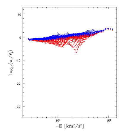
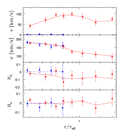
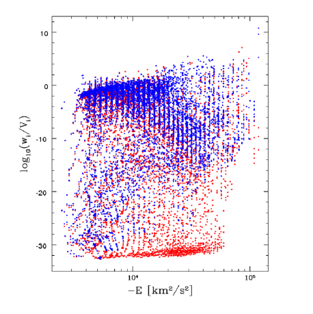
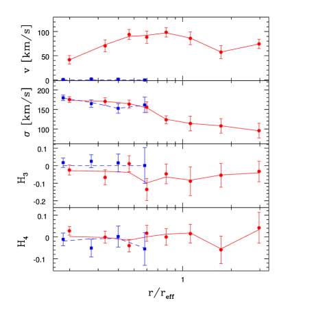
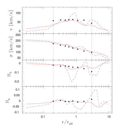
The DF at $\alpha=6.73$ has density depressions of several orders of magnitude for orbits with roughly the same energy. Orbit models with such DFs are difficult to interpret as the result of relaxation processes like violent relaxation and others, occurring in the dynamical evolution of real galaxies (e.g. Lynden-Bell 1967). They often predict uncommon kinematics along position angles not covered by observational data. To illustrate this, the projected kinematics predicted along a diagonal axis (position angle $\vartheta=45\degr$) by the two DFs of Figs. 3 and 4 are plotted in Fig. 5. For comparison the (undisturbed) kinematics of the isotropic rotator model are also overplotted. The profiles of the almost non-regularized ($\alpha=6.73$) fit show large point-to-point variations, which cannot easily be reconciled with the scatter in real observations. Also, the mean deviation between the unregularized orbit superposition and the input isotropic rotator (IR) model are larger for the non-regularized one than for the regularized one, e.g. $\langle H_{3}^{\mathrm{IR}}-H_{3}\rangle=0.06$ for $\alpha=6.73$ compared with $\langle H_{3}^{\mathrm{IR}}-H_{3}\rangle=0.02$ for $\alpha=0.02$.

Figure 5: Projected kinematics of the two DFs of Figs. 3 and 4 along a diagonal axis with position angle $\vartheta=45\degr$. Solid lines: $\alpha=0.02$ ($\rightarrow$ Fig. 3); dashed lines: $\alpha=6.73$ ($\rightarrow$ Fig. 4); dots: kinematics of the isotropic rotator model. Note that the orbit superpositions were fitted to the model only along the major and minor axes.

The above example demonstrates the importance of regularization in the context of recovering internal dynamics of isotropic rotators from sparse data sets typical for our sample of Coma galaxies. For NGC 4807 we have determined the optimal amount of regularization by means of Monte-Carlo simulations of several such isotropic rotator models (see Sec. 4.2 below).

The DFs of isotropic rotator models are of the form $f=f(E,L_{z})$ and represent only a minority of all possible DFs, since they are constant along $I_{3}$. The choice of such reference models for galaxies like NGC 4807 (fast rotating, faint giant ellipticals) is observationally motivated (Kormendy & Bender, 1996) and further supported by the weak velocity anisotropy found in previous dynamical studies (e.g. Gerhard et al. 2001; see also Sec. 7 for the case of NGC 4807), implying only a mild dependence of the DF on $I_{3}$. For more luminous ellipticals (shaped primarily by velocity anisotropy) or lenticulars embedded in roundish halos other reference models should be explored. We will turn to this in a future publication.

4.2 Regularization from isotropic rotator models

The isotropic rotator models constructed to determine the optimal regularization with respect to the analysis of NGC 4807’s internal structure are based on the edge-on as well as the $i=50\degr$ deprojections. For numerical reasons, however, the models at $i=50\degr$ are forced to have isophotes close to pure ellipses by setting $a_{4}\equiv a_{6}$ for the deprojection. Six models have been probed, three at each of the inclinations $i=50,90\degr$: one self-consistent, one embedded in a LOG-halo and a third embedded in a NFW-halo. Kinematic profiles are calculated from higher order internal velocity moments (Magorrian & Binney, 1994) following the procedure described in Sec. 4.1. Orbit libraries are fitted to the kinematic profiles and the internal velocity moments reconstructed from the fits are compared with the original input-moments for various values of $\alpha$. The optimal balance between entropy maximization and $\chi^{2}$-minimization is revealed where the reconstructed internal velocity moments are closest to the input model.

Fig. 6 shows the results for a self-consistent model based on the $i=90\degr$-deprojection. The upper panel shows the rms difference $\Delta(\alpha)$ between original and reconstructed internal velocity moments (up to second order) as a function of the regularization parameter $\alpha$. The rms is evaluated between the innermost and outermost fitted data points, at all position angles $\vartheta$, including intermediate ones, not covered by data points. The lower panel illustrates the goodness of fit $\chi^{2}_{\mathrm{GH}}/N_{\mathrm{data}}$. Solid lines correspond to the mean obtained by fitting orbit models to 60 Monte-Carlo realizations of the simulated data. Shaded areas comprise the 68 per cent fraction of best reconstructions (upper panel) and 68 per cent fraction of best fitting solutions (lower panel), respectively.

The best results are obtained for $\alpha=0.02$, when internal kinematics of the fits follow the input moments to an accuracy of about 15 per cent in the mean. Lower $\alpha$ yield less accurate reconstructions since the orbit superpositions do not fit the data enough (see $\chi^{2}_{\mathrm{GH}}$ in the lower panel). For larger $\alpha$ on the other hand, the rms $\Delta(\alpha)$ increases, because the library starts to fit the noise in the data.

On average, the orbit models at $\alpha=0.02$ fit with $\chi^{2}_{\mathrm{GH}}/N_{\mathrm{data}}<1$. A proper normalization for $\chi^{2}_{\mathrm{GH}}$ is however hard to obtain, since we do not exactly know the number of free parameters in the library. For $\alpha=0$ this number is zero, because $\chi^{2}$ does not appear in equation (7) while for $\alpha\rightarrow\infty$ there are roughly as many free parameters as orbits in the library, because then $S$ becomes negligible in equation (7). Thus, we do not try to calculate a reduced $\chi^{2}$.

Figure 6: Match $\Delta(\alpha)$ of internal velocity moments and $\chi^{2}_{\mathrm{GH}}/N_{\mathrm{data}}$ of the Gauss-Hermite parameters as a function of the regularization parameter $\alpha$. Lines represent the mean over 60 fits to Monte-Carlo realizations of the isotropic rotator’s kinematic profiles; shaded regions encompass 68 per cent of the simulations closest to the corresponding minimum in $\Delta(\alpha)$ and $\chi^{2}_{\mathrm{GH}}/N_{\mathrm{data}}$, respectively.

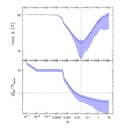
Table 1 summarizes the total of simulations done to fix $\alpha$. The first column labels the three models investigated at each of the two inclinations $i=50\degr$ and $i=90\degr$ (SC: self-consistent models without halo; LOG: a dark halo with $r_{c}=5\,\mathrm{kpc}$ and $v_{c}=265\,\mathrm{km/s}$ according to equation (2) is added to the stars; NFW: dark halo profile like in equation (3) with $r_{s}=10.0\,\mathrm{kpc}$, $c=27.0$; for all models $\Upsilon=3.0$). The halo models are constructed to produce a roughly flat circular velocity. In the second column of Table 1 the regularization $\alpha_{0}$ is quoted attaining the best reconstruction of the internal velocity moments, quantified in the third column as $\Delta(\alpha_{0})=\min(\Delta(\alpha))$. The corresponding goodness of fit $\chi^{2}_{\mathrm{GH}}(\alpha_{0})$ is given in the fourth column of the table. The number of orbits in each of the fitted libraries is found in the last column.

input model	$\alpha_{0}$	$\Delta(\alpha_{0})$	$\chi^{2}_{\mathrm{GH}}(\alpha_{0})$	$N_{\mathrm{orbit}}$
$i=90\degr$, SC	$0.0199$	$13.5\,\%$	$0.712$	$2\times 6922$
$i=90\degr$, LOG	$0.0166$	$12.7\,\%$	$0.719$	$2\times 8273$
$i=90\degr$, NFW	$0.0138$	$13.2\,\%$	$0.692$	$2\times 8469$
$i=50\degr$, SC	$0.0238$	$12.6\,\%$	$0.539$	$2\times 6697$
$i=50\degr$, LOG	$0.0166$	$13.8\,\%$	$0.826$	$2\times 8126$
$i=50\degr$, NFW	$0.0166$	$13.5\,\%$	$0.797$	$2\times 8324$

Table 1: Summary of simulations aimed at optimizing the regularization parameter $\alpha$. Columns from left to right: inclination of reference model; potential of reference model (SC = self-consistent, LOG = logarithmic spherical halo, NFW = spherical NFW-halo, details in the text); regularization parameter $\alpha_{0}$ that yields the best reconstruction of internal velocity moments; rms $\Delta(\alpha_{0})$ between internal velocity moments of reference models and reconstructions achieved with $\alpha=\alpha_{0}$; goodness of fit $\chi^{2}_{\mathrm{GH}}(\alpha_{0})$; number of orbits $N_{\mathrm{orbit}}$ used for the modeling.

On average, the six probed models yield $\langle\alpha_{0}\rangle=0.0179\pm 0.0035$. The low scatter seems to indicate that $\alpha_{0}$ does not depend strongly on the potentials tested. In the implementation of the maximum entropy technique used here, $\alpha$ is increased iteratively in discrete steps (see Richstone et al., in preparation). For the models of NGC 4807 we apply $\alpha=0.0199\approx 0.02$, which is the closest larger neighbor of $\langle\alpha_{0}\rangle$ in these iterations.

In the remainder of the paper, by quoting 68 (90, 95) per cent confidence levels, we always refer to all orbit models whose $\chi^{2}_{\mathrm{GH}}/N_{\mathrm{data}}$ are below the corresponding maximum $\chi^{2}$-level of the 68 (90, 95) per cent best-matching fits in the simulations. For these fits parameters like $\Upsilon$, $i$, $r_{c}$, $v_{c}$ …are set equal to the true input values, but in the analysis of real galaxies they are varied. Strictly speaking then, the $\chi^{2}$-statistics from the simulations are not directly applicable to real galaxies. For example, to determine the correct statistics for the case where $\Upsilon$, $r_{c}$ and $v_{c}$ are varied to find the best-fitting mass-model, about $10^{2}$ orbital fits for each triple of ($\Upsilon,r_{c},v_{c}$) are necessary to yield the corresponding three dimensional $\chi^{2}$-distribution. Such simulations however cannot be performed in a reasonable amount of time with present-day computer power.

Probably, our confidence regions derived as described above overestimate the error budget. For example, in the simulations we find 68 per cent of all orbits within $\Delta\chi^{2}_{\mathrm{GH}}/N_{\mathrm{data}}=0.38$ from the mean best-fit values. In contrast, applying classical $\Delta\chi^{2}$-statistics for a two parameter fit, yields about 95 per cent confidence at the same $\Delta\chi^{2}_{\mathrm{GH}}/N_{\mathrm{data}}=0.38$.

5 Recovering isotropic rotator models

The aim of this Section is to quantify in a practical sense to which degree a sparse data set like the one described in Sec. 2.3 constrains the internal kinematics and mass structure of a typical galaxy in our sample.

5.1 Mass-to-light ratio $\Upsilon$ and inclination $i$

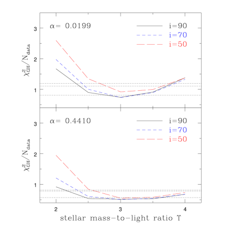
First, we disregard the possible presence of a dark halo and try to recover the mass-to-light ratio and inclination of the self-consistent edge-on model in Table 1. Therefore, Fig. 7 resumes the results of fitting libraries with mass-to-light ratios in the range $2.0\leqslant\Upsilon\leqslant 4.0$ and inclinations $i=50,70,90\degr$ to the kinematics of this isotropic rotator model. The goodness of fit $\chi^{2}_{\mathrm{GH}}/N_{\mathrm{data}}$ for each pair ($\Upsilon,i$) is averaged over 10 Monte-Carlo realizations of the kinematic profiles and evaluated at two different regularizations. For the upper panel $\alpha=0.02$ according to the simulations described in Sec. 4.2. Horizontal dotted lines in the plot correspond to 68, 90 and 95 per cent confidence levels as derived from the statistics of the simulations in Sec. 4.2.

One can read from the plot that the mass-to-light ratio is well recovered: the orbital fits reveal $\Upsilon=3.0\pm 0.5$, where the input model has $\Upsilon_{\mathrm{IR}}=3.0$. The minimum $\chi^{2}_{\mathrm{GH}}$ occurs at the true value independent of the assumed inclination. The latter is only weakly constrained. For $\Upsilon=3.0$ an inclination of $i=70\degr$ results in nearly the same $\chi^{2}_{\mathrm{GH}}/N_{\mathrm{data}}$ as the fit with the input $i_{\mathrm{IR}}=90\degr$. Even the orbit models with $i=50\degr$ can only be rejected with less than 90 per cent confidence.

For the lower panel the fits are evaluated at $\alpha=0.44$ (this choice of $\alpha$ is motivated in Sec. 6). Although at this less restrictive regularization the confidence intervals shrink as compared with $\alpha=0.02$ the mass-to-light ratio is now less constrained, $\Upsilon=3.0\pm 1.0$. The same holds for the inclination: at $\Upsilon=3.0$ all three probed inclinations are now within the 68 per cent confidence interval.

Figure 7: $\chi^{2}_{\mathrm{GH}}$ per data point ($N_{\mathrm{data}}=48$) as function of stellar $M/L$ for three different inclinations $i$. Top panel: with optimal smoothing, bottom panel: weak smoothing. The input 2I-model has $M/L=3.0$ and is edge-on. Pointed horizontal lines in each panel represent the $\chi^{2}_{\mathrm{GH}}$ values enclosing 68, 90 and 95 per cent of the Monte-Carlo simulations, respectively.

5.2 Internal kinematics

To give an impression about the ability to recover internal motions (assuming the potential is known) Fig. 8 compares internal velocity moments reconstructed from libraries fitted to the self-consistent edge-on isotropic rotator model of Sec. 4.1 with the corresponding moments of the input model. Solid lines portray the isotropic rotator model and points show the average reconstructed moments from fits to 60 Monte-Carlo simulations of the kinematic profiles; error bars indicate $1\,\sigma$ deviations from the mean. For the reconstructions $\alpha=0.02$ is used.

The three upper rows demonstrate that for the internal major axis the second order moments $\sigma_{R}$, $\sigma_{z}$ and $\sigma_{\varphi}$ are accurately reproduced by the fit over the region between the pointed vertical lines indicating the radii of the innermost and outermost kinematical points included in the fit. The fractional errors of $\sigma_{R}$ and $\sigma_{\varphi}$ are below 3 per cent and of $\sigma_{z}$ are below 6 per cent. For the internal rotation velocity $v_{\varphi}$ the fractional errors are larger than 10 per cent at some points. The match of the rotation velocity can be increased when going to larger $\alpha$, but then the second order moments start to wiggle around the input moments and the overall match of reconstructed to original moments becomes worse. Fig. 8 is representative also for the remaining internal position angles of the libraries. It follows that most of the rms in Fig. 6 results from a mismatch in $v_{\varphi}$.

Figure 8: Internal velocity moments along the major axis of libraries fitted to the self-consistent edge-on isotropic rotator model of Sec. 4.1. Dots: mean from fits to 60 Monte-Carlo realizations of the kinematic data; shaded regions: $1\,\sigma$ deviation from the mean; solid lines: velocity moments of the input model; dotted lines: boundaries of the radial region included in the fit.

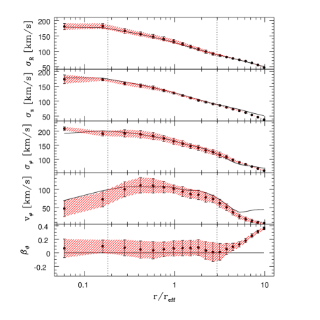
The last row shows a comparison of the anisotropy parameter $\beta_{\vartheta}=1-\sigma_{\vartheta}^{2}/\sigma_{r}^{2}$, which vanishes for isotropic rotator distribution functions $f=f(E,L_{z})$. The reconstructions are consistent with $\beta_{\vartheta}=0$ given the scatter caused by the noisy data. The small offset of $\Delta\beta_{\vartheta}=0.05$ is due to a slight overestimation of the radial velocity dispersion and emphasizes how sensitive $\beta_{\vartheta}$ responds to small inaccuracies in the velocity dispersions.

5.3 Mass distribution

The next step is to recover the structure of the isotropic rotator model in the second row of Table 1, where a logarithmic dark halo is present. To this end, we fitted libraries with different dark halos to pseudo data sets of the rotator model, keeping the stellar mass-to-light ratio constant. Fig. 9 combines the results of the simulations. It shows, from top to bottom, cumulative mass-to-light ratio $M(r)/L(r)$, circular velocity $v_{\mathrm{circ}}(r)$ and dark matter fraction $M_{\mathrm{DM}}(r)/M(r)$ as a function of radius. Vertical dotted lines mark the boundaries of the spatial region covered with kinematic data, thick lines display the input model. The shaded areas have been constructed by determining at each radius the minimum and maximum of $M/L$, $v_{\mathrm{circ}}$ and $M_{\mathrm{DM}}/M$ of all libraries within the 68 per cent confidence range derived from the simulations of Sec. 4.2. Libraries with LOG-halos as well as NFW-halos have been tried (see below) and for each library fits to 10 realizations of the isotropic rotator kinematics were averaged.

The figure demonstrates that in the region covered by the data the mass structure of the input model is well reproduced, with progressively larger scatter towards the outer edge of the data. The uncertainty of the mass-to-light ratio is $\Delta M/L\approx 1.0$ at $1\,r_{\mathrm{eff}}$, the circular velocity is accurate to 10 per cent at the same central distance. In the outer parts orbit superpositions with larger masses than the input model are better consistent with the data than smaller mass models. Nevertheless, the dark matter fraction is determined to $\Delta(M_{\mathrm{DM}}/M)=0.2$ even at the outermost data point.

Figure 9: Accuracy of the mass reconstruction. Thick lines: the isotropic rotator model marked by the asterix in Fig. 10; shaded areas: 68 per cent confidence regions of fits to pseudo data sets of the model. For each mass-model the goodness-of-fit is averaged over 10 fits to MC-realizations of pseudo-data.

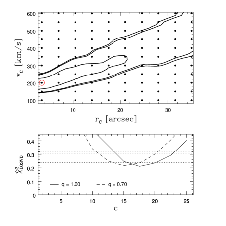
The top panel of Fig. 10 displays 68, 90 and 95 per cent confidence intervals for the two parameters $r_{c}$ and $v_{c}$ of LOG-halos (cf. equation 2). Each dot marks a pair of ($r_{c},v_{c}$) probed by fitting a library to 10 realizations of the pseudo-data as described above. The input model’s dark halo parameters are marked by the asterix, the circle designates the best-fitting orbit model.

As expected, the halo parameters are not well constrained. Although the best-fitting parameter pair is close to the input model, the 68 per cent confidence contour comprises a large set of libraries and remains open to the upper right edge of the plot. This follows from a degeneracy between the two parameters $r_{c}$ and $v_{c}$ (e.g. Gerhard et al. 1998). Increasing $r_{c}$ and $v_{c}$ appropriately puts more mass in the outer parts of the halos while rendering the regions covered by kinematics roughly unchanged. The increasing width of the shaded areas in the upper two panels of Fig. 9 is an illustration of this degeneracy.

We also fitted one parameter NFW-halos according to equation (5) to the same isotropic rotator model in order to examine whether these profiles can be excluded by the data set at hand. The lower panel of Fig. 10 displays the results in terms of $\chi^{2}_{\mathrm{GH}}/N_{\mathrm{data}}$ as a function of concentration index $c$. Horizontal dotted lines correspond to 68, 90 and 95 per cent confidence levels, the solid line shows fits with spherical halos ($q=1.0$), while for the dashed line $q=0.7$. Apparently, neither the halo flattening nor the central halo density slope are constrained by the data, because both spherical as well as flattened NFW-halos exist that provide fits equally as good as the LOG-halos. These NFW-halos join smoothly to the mass-distribution recovered in Fig. 9 and mimic LOG-halos over the limited spatial region covered by kinematic data.

Figure 10: Recovering an isotropic rotator model’s dark halo: $r_{c}$ and $v_{c}$ of the input model model are marked by the asterix in the top panel, the best-fit reconstruction is marked by the circle. Lines in the top panel display 68, 90 and 95 per cent confidence contours of the fits. The lower panel shows – for the same input model – $\chi^{2}$ of NFW-type fits (solid/dashed: $q=1.0$/$q=0.7$); horizontal lines: 68, 90 and 95 per cent confidence levels. Each library has been fitted to 10 realizations of the input-model kinematics.

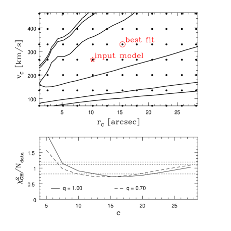
Fig. 10 suggests that it is not possible to discriminate between LOG and NFW halos insofar as they provide similar mass distributions over the spatial region sampled by kinematic data. More extended data sets are likely to reduce this degeneracy, but will probably not completely remove it. On the other hand, as Fig. 9 reveals, the mass distribution and composition of the input model can be recovered well, independently of the specific parameterization chosen to emulate it.

6 Dark matter in NGC 4807

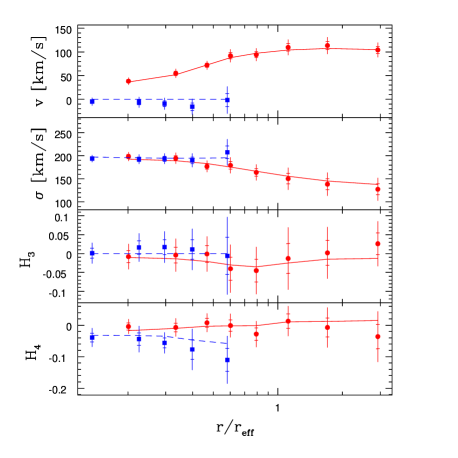
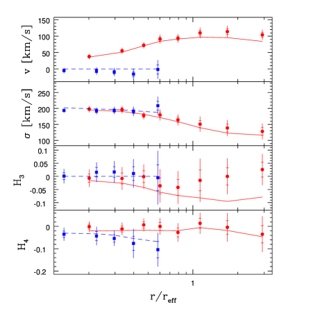
Now, we turn to the analysis of the distribution of luminous and dark mass in NGC 4807. Fig. 11 shows the minimum $\chi^{2}_{\mathrm{GH}}/N_{\mathrm{data}}$ (scaled, see below) at each modelled stellar mass-to-light ratio $\Upsilon\in\{1.0,2.0,2.5,3.0,3.5,4.0,5.0\}$. Horizontal lines indicate the 68, 90 and 95 per cent confidence limits derived from the simulations of Sec. 4.2. For the upper panel $\alpha=0.02$ is used and LOG-potentials with stellar mass-to-light ratios $2.5\leqslant\Upsilon\leqslant 3.0$ fit best to the data. Projected kinematics of the best-fitting orbit model are plotted in the upper panel of Fig. 12 together with the data. The model is edge-on, has stellar $\Upsilon=3.0$ and a spherical dark halo of LOG-type with core radius $r_{c}=6.8\,\mathrm{kpc}$ and asymptotic circular velocity $v_{c}=300\,\mathrm{km/s}$. It fits the data very well with (unscaled) $\min(\chi^{2}_{\mathrm{GH}}/N_{\mathrm{data}})=0.17$, even too well when compared with the average $\langle\chi^{2}_{\mathrm{GH}}/N_{\mathrm{data}}\rangle=0.71$ expected from the Monte-Carlo simulations. Since both, the scatter in the kinematic data from different sides of the galaxy (cf. Sec. 2.3) and the point-to-point variations in the profiles are smaller than the statistical error bars, the latter might be slightly overestimated. Hence, in the following all $\chi^{2}_{\mathrm{GH}}/N_{\mathrm{data}}$ are rescaled such that $\min(\chi^{2}_{\mathrm{GH}}/N_{\mathrm{data}})=\langle\chi^{2}_{\mathrm{GH}}/N_{\mathrm{data}}\rangle$. The good match of model and data nevertheless reconfirms that NGC 4807 is consistent with axisymmetry.

Applying regularization with $\alpha=0.02$, self-consistent models (mass follows light) are ruled out by more than $95$ per cent confidence (see thin solid line in the upper panel of Fig. 11). The best-fitting self-consistent model fits with (rescaled) $\chi^{2}_{\mathrm{GH}}/N_{\mathrm{data}}=1.67$ and is compared with the data in the bottom panel of Fig. 12. It has $\Upsilon=3.5$, larger than the best-fitting halo model, but fails to reach the measured rotation in the outer parts of the galaxy. A drop in the outer major axis $H_{3}$-profile indicates that the model maintains the measured dispersion $\sigma$ around the observed $v$ partly by putting light on retrograde orbits. This causes the LOSVD to fall off too sharply at velocities larger than $v$ and to develop a wing at negative velocities, resulting in the too negative $H_{3}$. Lack of support for dispersion at large rotation velocities hints at mass missing in the outer parts of this model. Higher mass-to-light ratios, however, would strengthen the mismatch between the central regions of the model and the innermost (minor axis) velocity dispersions.

Figure 11: Deviations between the observed kinematics of NGC 4807 and the fitted libraries in terms of $\chi^{2}_{\mathrm{GH}}$ as a function of $\Upsilon$. At each $\Upsilon$ the minimum $\min(\chi^{2}_{\mathrm{GH}})$ is plotted, separately for the case of LOG-halos (thick solid line), one-parameter NFW-halos (thick dashed) and for the self-consistent case (thin solid). For the top row the regularization parameter is $\alpha=0.02$, for the bottom row $\alpha=0.45$.

To push the self-consistent model to the same level of agreement with the data reached in the upper panel of Fig. 12, regularization must be lowered to $\alpha=0.45$. Although the best-fitting self-consistent model then gives a satisfactory fit in the sense of a reasonable $\chi^{2}_{\mathrm{GH}}/N_{\mathrm{data}}$, it is again ruled out by more than $95$ per cent confidence when compared with the mean $\langle\chi^{2}_{\mathrm{GH}}/N_{\mathrm{data}}\rangle$ using the Monte-Carlo simulations. This, because halo models at $\alpha=0.45$ still give significantly better fits to the data. The only effect of lower regularization – as shown in the run of $\chi^{2}_{\mathrm{GH}}/N_{\mathrm{data}}$ versus $\Upsilon$ in the lower panel of Fig. 11 – is a slight broadening of the minimum region in $\chi^{2}_{\mathrm{GH}}/N_{\mathrm{data}}$ and, consequently, an expansion of the allowed range of mass-to-light ratios, yielding now $2.0\leqslant\Upsilon\leqslant 3.5$ as compared with $2.5\leqslant\Upsilon\leqslant 3.0$ at $\alpha=0.02$. Concluding, NGC 4807 cannot be convincingly modelled with self-consistent orbit models, even at weak regularization.

Figure 12: Comparison of NGC 4807 (dots: major axis kinematic data; squares: minor axis) with the overall best-fitting model (upper panel) and best-fitting self-consistent model (lower panel). Both orbit models are at $i=90\degr$. For each data point two error bars are given: the statistical error from the observational data (larger, without marks) and the error bar corresponding to the scaled $\chi^{2}_{\mathrm{GH}}$ (marks).

In Fig. 13 (from top to bottom) the 68 per cent confidence regions of cumulative mass-to-light ratio $M(r)/L_{R}(r)$, circular velocity $v_{\mathrm{circ}}$ and dark matter fraction $M_{\mathrm{DM}}(r)/M(r)$ are shown (analogue to Fig. 9). Within 1 $r_{\mathrm{eff}}$ dark matter is negligible and the dynamical mass-to-light ratio equals the stellar one, $M(r)/L_{R}(r)=\Upsilon=3.0$. Between $1\,r_{\mathrm{eff}}$ and $3\,r_{\mathrm{eff}}$ dark matter comes up from $M_{\mathrm{DM}}/M=0.21\pm 0.14$ to $M_{\mathrm{DM}}/M=0.63\pm 0.13$ and combines with the luminous matter to a roughly flat circular velocity curve with $v_{\mathrm{circ}}=280\pm 30$ km/s at $1\,r_{\mathrm{eff}}$ and $v_{\mathrm{circ}}=318\pm 48$ km/s at the last kinematic data point. In the same spatial region the total mass-to-light ratio rises from $M(r)/L_{R}(r)=3.8\pm 0.8$ to $M(r)/L_{R}(r)=8.4\pm 2.4$. Dark mass equals luminous mass at roughly two effective radii. Beyond the last kinematic data point, the models are not well constrained and the profiles start to diverge.

Figure 13: Mass-structure of NGC 4807. Shaded regions are constructed as for Fig. 9. In the middle panel, the circular velocity curve of the best-fitting orbit model (solid line) and its decomposition into the stellar (dotted) and dark matter part (dashed) are displayed.

In accordance with the isotropic rotator simulations the halo parameters $r_{c}$ and $v_{c}$ are not well constrained – demonstrated by the $68$, $90$ and $95$ per cent confidence contours in Fig. 14. The tilted contour cones are narrower than expected from Fig. 10. Note however, that we have rescaled the $\chi^{2}_{\mathrm{GH}}$ and hence effectively reduced the error bars as compared with the simulations. Therefore, also the shaded areas in Fig. 13 are smaller than the corresponding in Fig. 9.

Figure 14: As Fig. 10, but for libraries fitted to the kinematics of NGC 4807. The best-fitting LOG-model is designated by the ring. In the lower panel results for spherical (solid line) as well as flattened NFW halos are illustrated (dashed line: $q=0.7$).

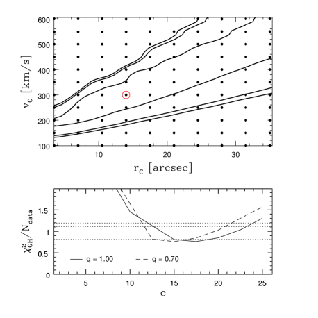
In the lower panel of Fig. 14 the goodness of fit $\chi^{2}_{\mathrm{GH}}/N_{\mathrm{data}}$ is plotted versus concentration $c$ for the one parameter family of NFW-profiles. As in the simulations of Sec. 5.3, the halo flattening is not constrained and with a best-fit $\chi^{2}_{\mathrm{GH}}/N_{\mathrm{data}}\approx 0.77$ spherical as well as flattened NFW-halos provide almost indistinguishable good fits to the data as the best-fitting LOG-halos. In the innermost regions of those libraries that match the observations, we find $\rho/\rho_{\mathrm{DM}}>10$; the logarithmic density slope of the best-fitting spherical NFW model is $\gamma=-1.8$ at the outermost major-axis data point and $\gamma=-2.41$ at the outer edge of the orbit library. Hence, as already pointed out in Sec. 5.3, the mass distributions of the data-allowed NFW models – over the modelled spatial region – resemble halos of LOG type. Fig. 15 illustrates the data-allowed range of dark matter densities along the major axis. Note that the lower limit on $\rho_{\mathrm{DM}}$ is likely due to the limited range of profile shapes probed in our study. Dark matter distributions with negative central density slopes $\gamma<0$ (not tested here) might also provide acceptable orbit models.

Figure 15: Major-axis stellar mass-density according to the edge-on deprojection (solid line, $\Upsilon=3.0$) and data allowed dark matter densities. Both, LOG and NFW-halos are included in the plot. (The shaded area is constructed analogously to Fig. 9.)

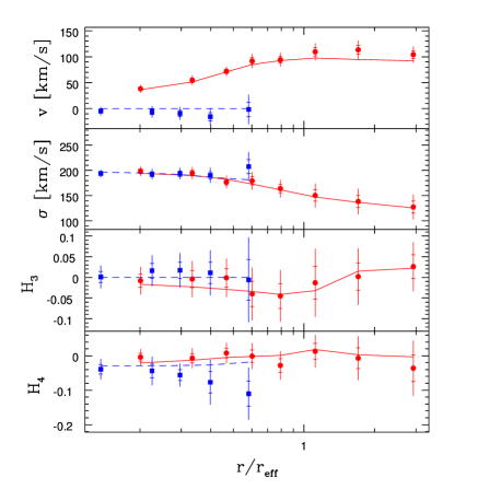
Models at $i=50\degr$ are ruled out by more than $68$, but less than $90$ per cent confidence. The best-fitting case is confronted with the kinematic observations in Fig. 16. Representative for all low-inclination models, it fails to reproduce the minor-axis $H_{4}$-profile, but the mass structure of this model joins to the profiles in Fig. 13 and the inferred structural properties of the galaxy are robust against the assumed inclination.

Figure 16: As Fig. 12, but for the best-fitting model at $i=50\degr$.

7 Stellar motions in NGC 4807

Visual inspection of the surfaces of section reveals that none of the orbit libraries for NGC 4807 contains a significant fraction of chaotic orbits. In the best-fitting models, at all inclinations, no indication for chaos is detectable at all.

The internal orbital structure of the best-fitting edge-on halo model near the major and minor axes is shown in Fig. 17. Around the equatorial plane, at radii $1\,r_{\mathrm{eff}}<r<3\,r_{\mathrm{eff}}$, the model is characterized by radial anisotropy. Enhanced radial velocity dispersion $\sigma_{r}$ causes $\beta_{\vartheta}\approx\beta_{\varphi}\approx 0.3$, whereas $\sigma_{\vartheta}\approx\sigma_{\varphi}$. Taking the large rotation velocity into account, energy in azimuthal motion turns out to be roughly equal to the energy in radial motion, $\langle v^{2}_{\varphi}\rangle\equiv v_{\mathrm{rot}}^{2}+\sigma_{\varphi}^{2}\approx\sigma^{2}_{r}$. On the other hand, motion perpendicular to the equator is suppressed. Approaching the central parts the velocity structure changes to isotropy and inside $r<0.5\,r_{\mathrm{eff}}$ stays isotropic.

Close to the minor axis, NGC 4807 appears nearly isotropic in the outer parts $1\,r_{\mathrm{eff}}<r<3\,r_{\mathrm{eff}}$ with decreasing radial dispersion towards the center, such that $\beta_{\vartheta}\approx\beta_{\varphi}<-0.5$ inside $r<0.5\,r_{\mathrm{eff}}$.

Figure 17: Internal kinematics of the best-fitting halo model near the major axis (top panel; position angle $\vartheta=2.9\degr$) and near the minor axis (bottom panel; $\vartheta=77.1\degr$), respectively. From top to bottom: velocity dispersions $\sigma_{r}$ (solid), $\sigma_{\vartheta}$ (short-dashed) and $\sigma_{\varphi}$ (long-dashed); velocity anisotropy $\beta_{\vartheta}$, $\beta_{\varphi}$; internal rotational velocity $v_{\mathrm{rot}}=v_{\varphi}$. Vertical, dotted lines indicate the innermost and outermost radius of kinematic data. Note, that the minor axis data reach only out to $0.6\,r_{\mathrm{eff}}$.

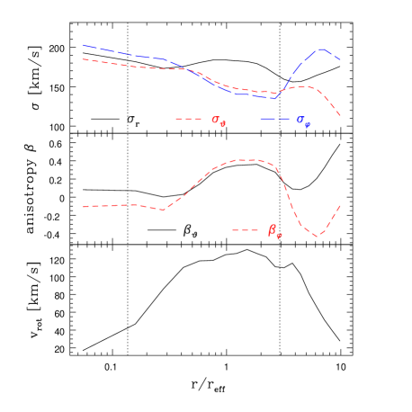
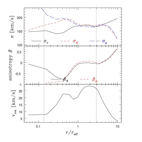
$68$ per cent confidence intervals analogous to Fig. 9 for velocity anisotropies $\beta_{\vartheta}$ and $\beta_{\varphi}$ as well as internal rotation velocities near the major and minor axes are shown in Fig. 18. Most tightly constrained is the major-axis rotation, rising from the central parts outwards until settling constant between $r_{\mathrm{eff}}$ ($v_{\mathrm{rot}}=124\pm 6$ km/s) and $3\,r_{\mathrm{eff}}$ ($v_{\mathrm{rot}}=107\pm 4$ km/s). Velocity anisotropy is determined to at least $\Delta\beta\leq 0.2$ and the trends in the anisotropy structure of the best-fitting model in Fig. 17 are clearly seen in all allowed orbit models.

Figure 18: Confidence regions for meridional velocity anisotropy $\beta_{\vartheta}$, azimuthal velocity anisotropy $\beta_{\varphi}$ and internal rotational velocity $v_{\mathrm{rot}}$ (upper panel: near major axis, position angle $\vartheta=2.9\degr$; lower panel: near minor axis, position angle $\vartheta=77.1\degr$) of NGC 4807. Shaded areas are constructed as for Fig. 9.

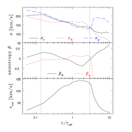
Fig. 19 illustrates the internal close-to-major axis kinematics of the best-fitting orbit model at $i=50\degr$. In contrast to the edge-on models $\beta_{\vartheta}\approx 0$ over almost the whole region constrained by observations, with a slight raise towards the center. Isotropy in the meridional plane ($\sigma_{r}\approx\sigma_{\vartheta}$) is accompanied by suppressed azimuthal dispersion $\sigma_{\varphi}$. But in contrast to the edge-on model of Fig. 17, the rotation of the actual model causes $\langle v^{2}_{\varphi}\rangle/\sigma^{2}_{r}\approx 1.7$, so that this model is dominated by azimuthal motion near the equatorial plane.

Figure 19: Internal close-to-major axis kinematics (position angle $\vartheta=2.9\degr$) of the best-fitting orbit model at $i=50\degr$. Line definitions as in Fig. 17.

8 Phase-space structure of NGC 4807

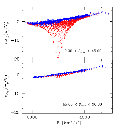
In Fig. 20 phase-space densities $w_{i}/V_{i}$ of individual orbits are plotted against orbital energy $E$ for the best-fitting orbit model of NGC 4807. The top panel only includes orbits whose maximally reached latitude, $\vartheta_{\mathrm{max}}$, is lower than $\vartheta_{\mathrm{max}}<45\degr$. These orbits are confined to a cone with opening angle $\vartheta<45\degr$ around the equatorial plane. The remaining orbits are plotted separately in the bottom panel. As in Figs. 3 and 4 the phase-space densities are scaled according to $\sum w_{i}=\sum V_{i}=1$, where $w_{i}$ and $V_{i}$ are the orbital weights and orbital phase volumes, respectively. Whereas the orbits maintaining the bulge of the galaxy follow a DF similar to the one shown in Fig. 3, some of the orbits confined around the equatorial plane are strongly depopulated. Around $E\approx 3000\,\mathrm{km}^{2}/\mathrm{s}^{2}$ phase-space densities are up to 20 orders of magnitude below the main stream DF.

Figure 20: Reconstructed distribution function of the best-fitting orbit model at $\alpha=0.02$. Each dot represents the phase-space density along a single orbit. Upper row: orbits confined to a konus with opening-angle $\vartheta_{\mathrm{max}}<45\degr$ around the equator; lower row: remaining orbits.

In the upper panel of Fig. 21 orbital phase densities are plotted against maximum orbital elongation $\vartheta_{\mathrm{max}}$ in the meridional plane. The three rows show orbits located in three different spatial regions separately. The top row includes only orbits whose invariant curves in the surface of section are confined to $0.5\,r_{\mathrm{eff}}<r_{\mathrm{SOS}}<1\,r_{\mathrm{eff}}$. The spatial regions for the other two rows are $1\,r_{\mathrm{eff}}<r_{\mathrm{SOS}}<2\,r_{\mathrm{eff}}$ and $2\,r_{\mathrm{eff}}<r_{\mathrm{SOS}}<4\,r_{\mathrm{eff}}$, respectively. Crosses denote orbits with positive $L_{z}>0$ while open circles denote orbits with negative $L_{z}<0$. From the center outwards, orbits with negative angular momentum are progressively depopulated as compared with their counterparts at positive $L_{z}$. The difference between prograde and retrograde orbits is most noticeable near the equatorial plane and disappears completely for bulge orbits reaching up to higher latitudes. In the bottom panel of Fig. 21 orbital phase densities are plotted against $L_{z}/L_{z,\mathrm{circ}}$, $L_{z,\mathrm{circ}}$ being the angular momentum of a circular orbit with the actual energy. Phase-space densities are extracted in the same spatial regions as for the upper panel of the Figure. It is now apparent that the keel in the DF of Fig. 20 is caused by a depopulation of (retrograde) circular orbits (at $|L_{z}|\approx L_{z,\mathrm{circ}}$).

Figure 21: The same model as in Fig. 20. Top panel: phase densities versus maximum orbital elongation $\vartheta_{\mathrm{max}}$ in the meridional plane. Bottom panel: phase densities versus “circularity” ($L_{z}$ scaled by the angular momentum $L_{z,\mathrm{circ}}$ of a circular orbit with same energy). Crosses (open circles) denote orbits with positive (negative) $L_{z}$. Orbits are extracted from different spatial regions of the model as designated in the panels (see text for details). For each spatial region the number of prograde orbits (crosses) equals the number of retrograde orbits (open circles).

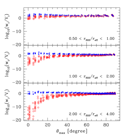
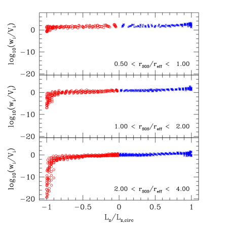
In fact, depopulation of retrograde near-circular orbits leading to the just described keel appears in all data-allowed DFs, with a slight tendency to be less pronounced in flattened halos. Even the DFs obtained assuming NGC 4807 is inclined by $i=50\degr$ are featured by this structure, albeit there, the keel is not exclusively made of retrograde orbits: also some of the prograde orbits are suppressed. In the low inclination DFs a third prominent substructure in phase-space emerges in form of a significant fraction of high-energy orbits (around $E\approx-2500\,\mathrm{km^{2}/s^{2}}$) being suppressed by about 6 orders of magnitude in density, independent from $L_{z}$. This structure partly overlays the keel and is caused by the distorted luminosity density at $i=50\degr$ since it shows up even in the maximum entropy models ($\alpha\approx 0$) which are only forced to reproduce the density profile, but not fitted to the kinematics.

Orbits in the keel together with their prograde counterparts (approximately all orbits $i$ with $w^{+}_{i}/w^{-}_{i}>99$, where $w^{\pm}_{i}\equiv w(E_{i},\pm L_{z,i},I_{3,i})$, $1\leq i\leq N_{\mathrm{pro}}$ and $N_{\mathrm{pro}}$ prograde orbits in the model) make only $4.3$ per cent of the total model. Without these orbits, a slowly rotating bulge ($v\approx 70\,\mathrm{km/s}$ at $r>r_{\mathrm{eff}}$) with a slightly peaked velocity distribution ($H_{4}>0.04$ at $r>r_{\mathrm{eff}}$) appears (see also Sec. 9.4). On the other hand, the extracted orbits rotate with about $200\,\mathrm{km/s}$ and produce a narrow, low-dispersion LOSVD. They develop a dumbbell-like structure extending to $2\,r_{\mathrm{eff}}$ above the equatorial plane. The fraction of extracted orbits additionally obeying $\vartheta_{\mathrm{max}}<10\degr$ shrinks to $0.7$ per cent of the total model.

9 Summary and Discussion

9.1 Regularized orbit models

We have investigated how closely the internal mass distribution and kinematic structure of a galaxy can be recovered from a sparse kinematic data set typical for our project aimed at investigating a sample of flattened early-type galaxies in the Coma cluster. The degree to which orbit models follow internal galaxy properties depends on the amount of regularization applied in the fits. In the maximum entropy technique of Richstone & Tremaine (1988) used here, a regularization parameter $\alpha$ controls the relative importance of entropy maximization (regularization) on the one side, and fit to the data on the other. To find out which choice of $\alpha$ is optimal with respect to our goal of determining galaxy structural parameters, we simulated observationally motivated isotropic rotator models under realistic observational conditions. The models are based on a prototypical elliptical in our sample, NGC 4807. By varying $\alpha$ in the fits of appropriate orbit libraries to pseudo data of the reference models, the match between internal velocity moments of input model and orbital reconstruction can be evaluated as a function of regularization.

Our simulations indicate that the mass-structure of an elliptical can be recovered to about 15 per cent accuracy in terms of mass-to-light ratio and circular velocity curve, if a regularization parameter $\alpha=0.02$ is applied. For the dynamical models tested here, the optimal choice of $\alpha$ turns out to be roughly independent from the galaxy’s gravitational potential. The same accuracy as for the mass structure is achieved in the reconstruction of internal velocity moments. On the other hand, halo flattening and galaxy inclination are only weakly constrained by our data.

Regularization biases orbit models towards some given idealized galaxy model, assumed to represent the object under study reasonably well. For early-type galaxies, regularization has been commonly implemented to isotropize the final fit. How much of regularization is optimal in the reconstruction of a given galaxy depends on the specific data set (spatial coverage, quality) on the one hand and the degree to which the regularization bias approximates the given galaxy on the other. Isotropizing the DF might, for example, be a good recipe for relaxed early-type galaxies but less favorable for lenticulars with a significant, dynamically cold, component. In that case either the value of $\alpha$ or, preferentially, the functional form of $S$ has to be reconsidered. In any case, and for any regularization technique, the optimal balance between fit to data and smoothing of the DF can be examined case-by-case from simulations similar to those described here.

Cretton et al. (1999) and Verolme & de Zeeuw (2002) have determined optimal regularization for an implementation of Schwarzschild’s method with two-integral components by reconstructing similar DFs as used here. The resulting regularization has proven to yield plausible results in subsequent applications (e.g. Cappellari et al. 2002; Verolme et al. 2002; Copin, Cretton & Emsellem 2004; Cretton & Emsellem 2004; Krajnović et al. 2005). It is difficult to quantitatively compare the amount of regularization applied in these works with the results of our simulations since the regularization techniques differ. However, in each case the achieved accuracy in the recovery of test model parameters and the derived dynamical structure of real galaxies indicate that the applied amount of regularization is comparable.

9.2 Luminous and dark matter in NGC 4807

We then applied our code with the simulation-derived regularization to the elliptical NGC 4807. The dynamical models require substantial dark matter in the outer parts of the galaxy. Evidence for dark matter in the form of flat circular velocity curves from (integrated) stellar kinematics of ellipticals has also been found by Rix et al. (1997), Gerhard et al. (1998), Emsellem, Dejonghe & Bacon (1999), Cretton, Rix & de Zeeuw (2000), Kronawitter et al. (2000), Saglia et al. (2000) and Gerhard et al. (2001). Dynamical models of five galaxies with planetary nebulae kinematics complementing stellar kinematics out to $\approx 5\,r_{\mathrm{eff}}$ lead the authors to different appraisals: Romanowsky et al. (2003) argue for non-dark matter models consistent with three galaxies observed by the planetary nebulae spectrograph, while Peng, Ford & Freeman (2004) require dark matter in NGC 5128 and the models of NGC 1399 also point at a dark halo (Saglia et al., 2000).

Spherical models for the 21 round ellipticals in the sample of Kronawitter et al. (2000) reveal dark matter fractions of $10-40$ per cent at $1\,r_{\mathrm{eff}}$ and dark mass equals luminous mass at roughly $2-4\,r_{\mathrm{eff}}$ (Gerhard et al., 2001), both comparable to our results for NGC 4807. The halo core density $\rho_{c}$ of our best-fitting model is about 30 per cent below the predictions of their $\rho_{c}-L_{B}$ relation (taking $M_{B}=-20.76$), although still consistent with it. Among the allowed LOG-halos however, the core densities vary by a factor of ten and taking into account NFW-fits, even halos $90$ times denser then the best-fitting model are consistent with the data (cf. Fig. 15). From the concentration of our best-fitting (spherical) NFW-halo nevertheless a relatively low formation redshift $z_{f}\approx 2.5$ follows. Still, we need a larger number of flattened ellipticals modelled in sufficient generality to recover the detailed properties and physical origin of their mass distributions.

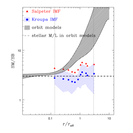
To crosscheck our mass decomposition for NGC 4807 we compared stellar mass-to-light ratios of the orbit superpositions with stellar mass-to-light ratios determined completely independent. In Fig. 22 mass-to-light ratios from stellar population models (Maraston 1998; Thomas, Maraston & Bender 2003; Maraston 2004) of NGC 4807’s major-axis spectrum (Mehlert et al. 2000; Mehlert et al. 2003) are compared to the best-fitting orbit models (dashed line: stellar mass-to-light ratio in orbit model; hatched region: 68 per cent confidence region of surface mass SM over surface brightness SB in orbit models; different symbols refer to different initial-mass-functions (IMFs) underlying the populations). Systematic uncertainties stemming from the unknown IMF are roughly comparable to the statistical errors, indicated for the Kroupa-IMF by the pointed area. Only libraries with $\Upsilon=3.0$ are taken into account in the figure.

As the figure demonstrates, the stellar mass-to-light ratios determined dynamically agree with stellar populations following a Kroupa IMF to $\Delta\Upsilon\approx 0.5$. This (1) confirms our mass decomposition and (2) justifies a posteriori the assumption of a constant stellar mass-to-light ratio. The total surface mass of the dynamical models, as indicated by the shaded region in Fig. 22, exceeds the stellar contribution by far and underlines the evidence for dark matter in NGC 4807. Since our best-fitting orbit models have LOG-halos (or NFW-halos imitating the mass distribution of LOG-halos over the kinematically sampled spatial region) they have maximum stellar mass (e.g. Gerhard et al. 1998). This is in accordance with most previous studies that did not require steep central dark matter profiles (Gerhard et al. 1998; Emsellem, Dejonghe & Bacon 1999; Cretton, Rix & de Zeeuw 2000; Kronawitter et al. 2000; Saglia et al. 2000 and Gerhard et al. 2001). On the other hand, Rix et al. (1997) found such profiles consistent with NGC 2434.

Figure 22: Projected mass-to-light ratio along the major axis of NGC 4807. Hatched area: 68 per cent confidence region of surface mass (SM) over surface brightness (SB) for all orbit models with $\Upsilon=3.0$ (dashed line). For comparison the projected stellar mass-to-light ratios from population analysis (see text) are shown for two different IMFs: Salpeter-IMF (triangles), Kroupa-IMF (dots). The pointed area encompasses the statistically allowed $\Upsilon$ based on the Kroupa-IMF. For the sake of clarity, the similar, but shifted, error region for the Salpeter-based $\Upsilon$ is omitted.

9.3 Comparing the kinematics: $\chi^{2}_{\mathrm{GH}}$ versus $\chi^{2}_{\mathrm{LOSVD}}$

The confidence intervals for the structural properties of NGC 4807 have been derived from $\chi^{2}_{\mathrm{GH}}$ as defined in equation (3.5). However, our models do not explicitly minimize $\chi^{2}_{\mathrm{GH}}$ but instead $\chi^{2}_{\mathrm{LOSVD}}$ as given by equation (8). In order to investigate how the properties of the best-fitting orbit model and the corresponding confidence limits of the halo parameters depend on the choice of $\chi^{2}$ we have analyzed the Monte-Carlo simulations as well as the models for NGC 4807 also in terms of

$$\hat{\chi}^{2}_{\mathrm{LOSVD}}\equiv\chi^{2}_{\mathrm{LOSVD}}/\hat{N}_{\mathrm{data}},$$ (11)

where $\hat{N}_{\mathrm{data}}$ is the number of velocity bins for which ${\cal L}^{jk}_{\mathrm{dat}}>0$ (cf. equation 8).

Fig. 23 shows the best-fitting halo parameters and corresponding confidence intervals for the simulated isotropic rotator model of Sec. 5.3. The figure is as Fig. 10, besides that all confidence regions and model-with-data comparisons are computed in terms of $\hat{\chi}^{2}_{\mathrm{LOSVD}}$. Comparing Figs. 10 and 23, it turns out that both $\chi^{2}$-definitions yield identical best-fitting models (designated by the rings in the upper panels, and given by the minima of the two curves in the lower panels). Concerning the confidence regions, however, the computations based on $\hat{\chi}^{2}_{\mathrm{LOSVD}}$ lead to smaller confidence limits for both, the logarithmic and the NFW-halos.

Figure 23: As Fig. 10, but the confidence regions are derived from $\hat{\chi}^{2}_{\mathrm{LOSVD}}$ (see Sec. 3.5).

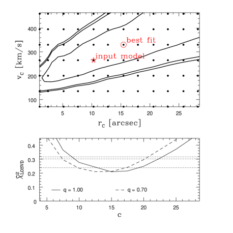
For NGC 4807, the analysis based on $\hat{\chi}^{2}_{\mathrm{LOSVD}}$ leads to the results shown in Fig. 24. Again, besides the different $\chi^{2}$-definition applied, it is as Fig. 14. The best-fitting NFW-halos in Fig. 24 are the same as in Fig. 14. The shapes of the $\hat{\chi}^{2}_{\mathrm{LOSVD}}$ curves for $q=1.0$ and $q=0.7$ in the bottom panel of Fig. 24 prefer halos slightly more concentrated than in the $\chi^{2}_{\mathrm{GH}}$-case, but, as for the isotropic rotator simulations, the differences in the results obtained from $\chi^{2}_{\mathrm{GH}}$ and $\hat{\chi}^{2}_{\mathrm{LOSVD}}$ are small.

Regarding the best-fitting logarithmic-halo models (marked by the rings in the upper panels) both $\chi^{2}$-calculations give consistent, but, in contrast to the Monte-Carlo simulations, not identical results. As already indicated in the NFW-fits, the logarithmic halo that best fits in the sense of $\hat{\chi}^{2}_{\mathrm{LOSVD}}$ is more concentrated: the dark matter fraction inside $r_{\mathrm{eff}}$ is $M_{\mathrm{DM}}/M=0.35$, compared with $M_{\mathrm{DM}}/M=0.22$ for the best-fitting model in the upper panel of Fig. 14. A more striking difference between the upper panels of Fig. 14 and 24 is the closure of the 68 per cent $\hat{\chi}^{2}_{\mathrm{LOSVD}}$-confidence contour to the upper right. The contour differences maybe related to the ignorance of $\gamma_{0}$ in equation (3.5), since the mismatch between model and data intensities progressively increases from the lower left to the upper right in the upper panel of Fig. 14.

Nevertheless, the comparison of the results obtained from $\chi^{2}_{\mathrm{GH}}$ and $\hat{\chi}^{2}_{\mathrm{LOSVD}}$ reveals that both methods – within the errors – give the same results. The confidence limits quoted in this paper, based on equation (3.5), are the more conservative choice, but maybe slightly too pessimistic.

Figure 24: As Fig. 14, but the confidence regions are derived from $\hat{\chi}^{2}_{\mathrm{LOSVD}}$ (see Sec. 3.5).

9.4 The outer parts of NGC 4807

Based on a recent refinement (Thomas et al., 2004) of the Schwarzschild code of Richstone & Tremaine (1988) and Gebhardt et al. (2000), we recovered a depopulation of retrograde, near-circular orbits in the phase-space DF of NGC 4807, giving rise to a keel when plotting orbital phase-space densities against orbital energy. The prograde counterparts of the depopulated orbits form a dumbbell-like structure extending about $\approx 2\,r_{\mathrm{eff}}$ above the equatorial plane.

Figure 25: Upper panel: projected major-axis kinematics of three distribution functions calculated in the gravitational potential of the best-fitting mass model: (1) all retrograde orbits in the keel depopulated completely (solid); relative fraction of light on prograde keel-orbit counterparts (2) $\xi=0.94$ (short-dashed) and (3) $\xi=0.7$ (dotted). Lower panel: goodness of fit (including the minor-axis LOSVDs, which are not affected by the redistribution of keel-involved orbits) as a function of the relative fraction $\xi$ of light on prograde keel-orbit correspondents; horizontal dotted lines indicate 68, 90 and 95 per cent confidence levels.

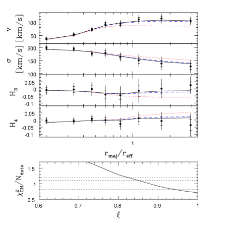
To investigate what might cause the depopulation of retrograde orbits in the outer parts of NGC 4807, we projected a sequence of distribution functions in which all orbits involved in the keel ($w^{+}_{i}/w^{-}_{i}>99$, see Sec. 8) are repopulated according to

$$\begin{array}[]{l}w^{+}_{i,\mathrm{new}}\equiv\xi\times\left(w^{+}_{i}+w^{-}_{i}\right)\\ w^{-}_{i,\mathrm{new}}\equiv(1-\xi)\times\left(w^{+}_{i}+w^{-}_{i}\right).\end{array}$$

Since $w^{+}_{i,\mathrm{new}}+w^{-}_{i,\mathrm{new}}=w^{+}_{i}+w^{-}_{i}$ this does not alter the fit to the luminosity profile but just levels the relative fraction $\xi$ of light on the prograde and retrograde specimen of all keel-involved orbit pairs. Roughly speaking, equation (9.4) transforms the keel into a narrow cloud of points parallel to the main-stream DF with an offset increasing with $|\xi-0.5|$. Figure 25 shows the resulting projected (major-axis) kinematics for $\xi=0.7,0.94,1.0$. As expected, shifting light from prograde to retrograde orbits reduces the amount of rotation $v$ and lowers $H_{3}$ in the outer parts, while at the same time leading to a larger velocity dispersion $\sigma$ and enhanced $H_{4}$. As shown by the goodness of fit in the lower panel of Fig. 25, the best fit to the data is achieved for $\xi=1.0$ (all retrograde keel-orbits completely depopulated). Comparing the corresponding solid lines in Fig. 25 with the upper panel of Fig. 12 reveals that $\xi=1.0$ provides essentially the same fit as the best-fitting orbit model. Consequently, the retrograde keel-orbits can be regarded as completely depopulated in our models of NGC 4807. Reducing the relative fraction of light on the prograde counterparts of keel-orbits to $\xi=0.94$ is only consistent with the observations at the 68 per cent confidence level. A further equalization to $\xi=0.7$ is already incompatible with the observed velocity profiles.

The outer major-axis LOSVDs of NGC 4807 might indicate weak triaxiality, for example in form of a weak, nearly end-on bar (e.g. Bureau & Athanassoula, 2004). A weak bar-like structure would also fit to the boxy appearance of the galaxy’s outer isophotes. Assuming that NGC 4807 is slightly triaxial, the keel in the DF might be an artifact of the assumption of axisymmetry. Note, however, that NGC 4807 is consistent with being axisymmetric, albeit then the depopulation of single orbit families, especially around the equatorial plane, is hard to understand in the course of dynamical processes.

Depopulation of retrograde orbits in the outer parts of the galaxy is accompanied by a change in stellar ages from $\tau\approx 5\,\mathrm{Gyr}$ inside $r<r_{\mathrm{eff}}$ to $\tau\approx 10\,\mathrm{Gyr}$ at larger radii (Mehlert et al., 2003). Towards $3\,r_{\mathrm{eff}}$ stellar ages become uncertain and no clear trend is visible. It seems also possible, that the keel in the DF is an artifact related to a distinct stellar component and an associated (slight) change in $\Upsilon$. It should be noted that because the orbit models are fitted to deprojections and stellar kinematics, the derived DFs characterize the amount of light per volume element in phase-space, not the mass-density in phase-space. Accordingly, depressions in the DF might (at least partly) reflect enhanced $\Upsilon$.

A distinct stellar component in the outer parts must not necessarily take the form of a bar, but could also be a faint axisymmetric stellar disk. Indeed, the photometry as well as the orbit models suggest that NGC 4807 is close to edge-on, but a dynamically cold, outer stellar disk made of only $0.7$ per cent prograde orbits at latitudes $\vartheta<10\degr$ (see Sec. 8) is consistent with the non-disky isophotes ($\max a_{4}<1$). A disk carrying 2 per cent of the total luminosity would show up with $\max a_{4}\approx 4$ when seen exactly edge-on and $\max a_{4}<1$ for such a disk would require $i<75\degr$ (Rix & White, 1990). From our simulations it seems impossible to distinguish kinematically between $i=70\degr$ and $i=90\degr$ and, consequently, there is some freedom for an outer disk in NGC 4807.

In any case further investigations are necessary to verify the significance of the keel-structure in the DF of NGC 4807. (1) Kinematic measurements along intermediate position angles in the galaxy would likely put more constraints on the DF. (2) Detailed comparison of orbit superpositions with realistic galaxy models are required to estimate how relics of triaxiality, faint disks and multi-component (multi-$\Upsilon)$ structures show up in our axisymmetric models. These questions will be addressed in a forthcoming publication.

9.5 Internal stellar kinematics of NGC 4807

Along the major-axis, NGC 4807 is mildly radially anisotropic. Radial anisotropy has been found in a number of ellipticals (Gerhard et al. 1998; Matthias & Gerhard 1999; Cretton, Rix & de Zeeuw 2000; Gebhardt et al. 2000; Saglia et al. 2000). The amount of anisotropy ($\beta\approx 0.3$) in the outer parts as well as the isotropy of the central region (inside $0.3\,r_{\mathrm{eff}}$) matches with the typical anisotropy structure found for round, non-rotating ellipticals by Gerhard et al. (2001). Along the minor axis, NGC 4807 is dominated by tangential motions. Gebhardt et al. (2003) report tangential anisotropy for some galaxies (mostly enhanced azimuthal, but suppressed meridional dispersions) and also Dejonghe et al. (1996), Cretton & van den Bosch (1998), Statler, Dejonghe & Smecker-Hane (1999), Cappellari et al. (2002), Verolme et al. (2002) and Copin, Cretton & Emsellem (2004) find predominantly tangential motions. For NGC 3115 Emsellem, Dejonghe & Bacon (1999) notice $\sigma_{z}>\sigma_{r}$. All these studies are based on data sets with different spatial sampling and use various dynamical modelling techniques, particularly differing in the amount and functional form of the applied regularization. As for the mass structure and the dark matter properties, a large and homogeneous sample of galaxies is needed to address the physical processes shaping elliptical galaxies.

References

- Bender & Möllenhoff (1987) Bender R., Möllenhoff C., 1987, A&A 177, 71
- Binney & Tremaine (1987) Binney J., Tremaine S., 1987, Galactic Dynamics (princeton: Princeton University Press)
- Bureau & Athanassoula (2004) Bureau M., Athanassoula E., 2004, preprint (astro-ph/0403226)
- Cappellari et al. (2002) Cappellari M., Verolme E. K., van der Marel R. P., Verdoes Kleijn G. A., Illingworth G. D., Franx M., Carollo C. M., de Zeeuw P. T., 2002, ApJ, 578, 787
- Carollo et al. (1995) Carollo C. M., de Zeeuw P. T., van der Marel R. P., Danziger I. J., Qian E. E., 1995, ApJL, 441, 25
- Colin, Avila-Reese & Valenzuela (2000) Colin P., Avila-Reese V., Valenzuela O., 2000, ApJ, 542, 622
- Copin, Cretton & Emsellem (2004) Copin Y., Cretton N., Emsellem E., 2004, A&A, 415, 889
- Cretton & van den Bosch (1998) Cretton N., van den Bosch F. C., 1998, ApJ, 514, 704
- Cretton et al. (1999) Cretton N., de Zeeuw P. T., van der Marel R. P., Rix H. W., 1999, ApJS, 124, 383
- Cretton, Rix & de Zeeuw (2000) Cretton N., Rix H. W., de Zeeuw P. T., 2000, ApJ, 536, 319
- Cretton & Emsellem (2004) Cretton N., Emsellem E., 2004, MNRAS 347, L31
- Davé et al. (2001) Davé R., Spergel D. N., Steinhardt P. J., Wandelt B. D., 2001, ApJ, 547, 574
- de Blok et al. (2001) de Blok W. J. G., McGaugh S. S., Bosma A., Rubin V. C., 2001, ApJL, 552, 23
- Dehnen & Gerhard (1994) Dehnen W., Gerhard O. E., 1994, MNRAS 268, 1019
- Dejonghe et al. (1996) Dejonghe H., de Bryne V., Vauterin P., Zeilinger W. W., 1996, A&A, 306, 363
- Emsellem, Dejonghe & Bacon (1999) Emsellem E., Dejonghe H., Bacon R., 1999, MNRAS, 303, 495
- Gebhardt et al. (2000) Gebhardt K. et al., 2000, AJ, 119, 1157
- Gebhardt et al. (2003) Gebhardt K. et al., 2003, ApJ, 583, 92
- Gentile et al. (2004) Gentile G., Salucci P., Klein U., Vergani D., Kalberla P., 2004, MNRAS, 351, 903
- Gerhard (1993) Gerhard O. E., 1993, MNRAS, 265, 213
- Gerhard & Binney (1996) Gerhard O. E., Binney J., 1996, MNRAS, 279, 993
- Gerhard et al. (1998) Gerhard O. E., Jeske G., Saglia R. P., Bender R., 1998, MNRAS, 295, 197
- Gerhard et al. (2001) Gerhard O. E., Kronawitter A., Saglia R. P., Bender R., 2001, AJ, 121, 1936
- Häfner et al. (2000) Häfner R., Evans N. W., Dehnen W., Binney J., 2000, MNRAS, 314, 433
- Jing & Suto (2000) Jing Y. P., Suto Y., 2000, ApJ, 529, L69
- Knebe et al. (2002) Knebe A., Devriendt J. E. G., Mahmood A., Silk J., 2002, MNRAS, 329, 813
- Kormendy & Bender (1996) Kormendy J., Bender R., 1996, ApJ, 464, 119
- Krajnović et al. (2005) Krajnović D., Cappellari M., Emsellem E., McDermid R. M., de Zeeuw P. T., 2005, MNRAS, 357, 1113
- Kronawitter et al. (2000) Kronawitter A., Saglia R. P., Gerhard O. E., Bender R., 2000, A&AS, 144, 53
- Lynden-Bell (1967) Lynden-Bell D., 1967, MNRAS, 136, 101
- Magorrian & Binney (1994) Magorrian J., Binney J., 1994, MNRAS, 271, 949
- Magorrian (1999) Magorrian J., 1999, MNRAS, 302, 530
- Maraston (1998) Maraston C., 1998, MNRAS, 300, 872
- Maraston (2004) Maraston C., 2004, preprint (astro-ph/0410207)
- Matthias & Gerhard (1999) Matthias M., Gerhard O. E., 1999, MNRAS, 310, 879
- Mehlert et al. (2000) Mehlert D., Saglia R. P., Bender R., Wegner G., 2000, A&AS, 141, 449
- Mehlert et al. (2003) Mehlert D., Thomas D., Saglia R. P., Bender R., Wegner G., 2003, A&A, 407, 423
- Merritt (1993) Merritt D. R., 1993, ApJ, 413, 79
- Moore et al. (1999) Moore B., Quinn T., Governato F., Stadel J., Lake G., 1999, MNRAS, 310, 1147
- Navarro, Frenk & White (1996) Navarro J. F., Frenk C. S., White S. D. M., 1996, ApJ, 462, 563
- Navarro et al. (2004) Navarro J. F. et al., 2004, MNRAS, 349, 1039
- Peng, Ford & Freeman (2004) Peng E. W., Ford H. .C, Freeman K. C., 2004, ApJ, 602, 685
- Qian et al. (1995) Qian E. E., de Zeeuw P. T., van der Marel R. P., Hunter C., 1995, MNRAS, 274, 602
- Richstone & Tremaine (1988) Richstone D. O., Tremaine S., 1988, ApJ, 327, 82
- Rix & White (1990) Rix H. W., White S. D. M., 1990, ApJ, 362, 52
- Rix et al. (1997) Rix H. W., de Zeeuw P. T., Cretton N., van der Marel R. P., Carollo C. M., 1997, ApJ, 488, 702
- Romanowsky et al. (2003) Romanowsky A. J., Douglas N. G., Arnaboldi M., Kuijken K., Merrifield M. R., Napolitano N. R., Capaccioli M., Freeman K. C., 2003, Sci, 301, 1696
- Rybicki (1987) Rybicki G., 1987, in de Zeeuw T., ed., Proc. IAU Symp. 127, Structure and Dynamics of Elliptical Galaxies, Reidel, Dordrecht, p. 397
- Saglia et al. (2000) Saglia R. P., Kronawitter A., Gerhard O. E., Bender R., 2000, AJ, 119, 153
- Schwarzschild’s (1979) Schwarzschild M., 1979, ApJ, 232, 236
- Statler, Dejonghe & Smecker-Hane (1999) Statler T. S., Dejonghe H., Smecker-Hane T., 1999, AJ, 117, 126
- Swaters et al. (2003) Swaters R. A., Madore B. F., van den Bosch F. C., Balcells M., 2003, ApJ, 583, 732
- Thomas, Maraston & Bender (2003) Thomas D., Maraston C., Bender R., 2003, MNRAS, 339, 897
- Thomas et al. (2004) Thomas J., Saglia R. P., Bender R., Thomas D., Gebhardt K., Magorrian J., Richstone D., 2004, MNRAS, 353, 391
- Valluri, Merritt & Emsellem (2004) Valluri M., Merritt D., Emsellem E., 2004, ApJ, 602, 66
- van der Marel & Franx (1993) van der Marel R. P., Franx M., 1993, ApJ, 407, 525
- Verolme et al. (2002) Verolme E. K. et al., 2002, MNRAS, 335, 517
- Verolme & de Zeeuw (2002) Verolme E. K., de Zeeuw P. T., 2002, MNRAS, 331, 959
- Wechsler et al. (2002) Wechsler R. H., Bullock J. S., Primack J. R., Kravtsov A. V., Dekel A., 2002, ApJ, 568, 52
- Wegner et al. (2002) Wegner G., Corsini E. M., Saglia R. P., Bender R., Merkl D., Thomas D., Thomas J., Mehlert D., 2002, A&A, 395, 753
- Zhao (1996) Zhao H. S., 1996, MNRAS, 283, 149