Model-Independent Multi-Variable Gamma-Ray Burst Luminosity Indicator and Its Possible Cosmological Implications

Abstract

Without imposing any theoretical models and assumptions, we present a multi-variable regression analysis to several observable quantities for a sample of 15 gamma-ray bursts (GRBs). The observables used in the analysis includes the isotropic gamma-ray energy ($E_{\gamma,{\rm{iso}}}$), the peak energy of the $\nu F_{\nu}$ spectrum in the rest frame ($E_{\rm{p}}^{{}^{\prime}}$), and the rest frame break time of the optical afterglow light curves($t_{\rm{b}}^{{}^{\prime}}$). A strong dependence of $E_{\gamma,{\rm iso}}$ on $E_{\rm p}^{{}^{\prime}}$ and $t_{b}^{{}^{\prime}}$ is derived, which reads $E_{\gamma,{\rm{iso}}}/10^{52}{\rm ergs}=(0.85\pm 0.21)\times(E^{{}^{\prime}}_{\rm{p}}/{\rm 100\ keV})^{1.94\pm 0.17}\times(t^{{}^{\prime}}_{\rm{b}}/1{\rm day})^{-1.24\pm 0.23}$ in a flat Universe with $\Omega_{M}=0.28$ and $H_{0}=71.3$ km s^-1 Mpc^-1. We also extend the analysis to the isotropic afterglow energies in the X-ray and the optical bands, respectively, and find that they are essentially not correlated with $E_{\rm{p}}^{{}^{\prime}}$ and $t_{\rm{b}}^{{}^{\prime}}$. Regarding the $E_{\gamma,{\rm{iso}}}(E_{\rm{p}}^{{}^{\prime}},t_{\rm{b}}^{{}^{\prime}}$) relationship as a luminosity indicator, we explore the possible constraints on the cosmological parameters using the GRB sample. Since there is no low-redshift GRB sample to calibrate this relationship, we weigh the probability of using the relationship in each cosmology to serve as a standard candle by $\chi^{2}$ statistics, and then use this cosmology-weighed standard candle to evaluate cosmological parameters. Our results indicate $0.05<\Omega_{\rm{M}}<0.50$ at $1\sigma$ level, with the most possible value of $\Omega_{\rm{M}}$ being $0.28$. The best value of $\Omega_{\Lambda}$ is 0.64, but it is less constrained. Only a loose limit of $\Omega_{\Lambda}<1.2$ is obtained at $1\sigma$ level. In the case of a flat Universe, the $1\sigma$ constraints are $0.13<\Omega_{\rm{M}}<0.49$ and $0.50<\Omega_{\Lambda}<0.85$, respectively. The decelerating factor ($q$) and its cosmological evolution $(dq/dz)$ are also investigated with an evolutionary form of $q=q_{0}+zdq/dz$. The best-fit values are $(q_{0},dq/dz)=(-1.00,1.12)$, with $-2.23<q_{0}<0.26$ and $-0.07<dq/dz<3.48$ at $1\sigma$ level. The inferred transition redshift between the deceleration and the acceleration phases is $0.78^{+0.32}_{-0.23}$ ($1\sigma$). Through Monte Carlo simulations, we find that the GRB sample satisfying our relationship observationally tends to be a soft and bright one, and that the contraints on the cosmological parameters can be much improved either by the enlargement of the sample size or by the increase of the observational precision. Although the sample may not expand significantly in the Swift era, a significant increase of the sample is expected in the long term future. Our similations indicate that with a sample of 50 GRBs satisfying our multi-variable standard candle, one can achieve a constraint to the cosmological parameters comparable to that derived from 157 Type Ia supernovae. Furthermore, the detections of a few high redshift GRBs satisfying the correlation could greatly tighten the constraints. Identifying high-$z$ GRBs and measuring their $E^{\prime}_{p}$ and $t^{\prime}_{b}$ are therefore essential for the GRB cosmology in the Swift era.

1. Introduction

Long gamma-ray bursts (GRBs) are originated from cosmological distances (Metzger et al. 1997). Their births follow the star formation history of the universe (e.g. Totani 1997; Paczynski 1998; Bromm & Loeb 2002; Lin et al. 2004). GRBs therefore promise to serve as a new probe of cosmology and galaxy evolution (e.g., Djorgovski et al. 2003). It is well known that Type Ia supernovae (SNe Ia) are a perfect standard candle to measure the local universe up to a redshift of $\sim 2$ (e.g., Riees et al. 2004). Gamma-ray photons (with energy from tens of keV to several MeV) from GRBs are almost immune to dust extinction. They should be detectable out to a very high redshift (Lamb & Reichart 2000; Ciardi & Loeb 2000; Gou et al. 2004). Hence, GRBs are potentially a more promising ruler than SNe Ia at higher redshifts.

This issue has attracted much attention in GRB community. Frail et al. (2001) found that the geometrically-corrected gamma-ray energy $E_{\rm{jet}}$ for long GRBs is narrowly clustered around $5\times 10^{50}$ ergs, suggesting that GRBs can be potentially a standard candle. A refined analysis by Bloom, Frail, & Kulkarni (2003a) suggests that $E_{\rm{jet}}$ is clustered at $1.3\times 10^{51}$ ergs, but the dispersion of $E_{\rm{jet}}$ is too large for the purpose of constraining cosmological parameters. Schaefer (2003) considered two other luminosity indicators proposed earlier, i.e. the variability (Fenimore & Ramirez-Ruiz 2000; Reichart et al. 2001) and the spectral lag (Norris, Marani, & Bonnell 2000), for nine GRBs with known redshifts, and pose an upper limit of $\Omega_{\rm{M}}<0.35$ ($1\sigma$) for a flat universe. Using 12 BeppoSAX bursts, Amati et al. (2002) found a relationship between the isotropic-equivalent energy radiated during the prompt phase ($E_{\gamma,{{\rm{iso}}}}$) and rest frame peak energy in the GRB spectrum ($E^{\prime}_{\rm{p}}$), i.e., $E^{\prime}_{\rm{p}}\propto E_{\gamma,{{\rm{iso}}}}^{1/2}$. This relation was confirmed and extended to X-ray flashes by HETE-2 observations (Sakamoto et al. 2004a; Lamb et al. 2005a). In addition, it also exists in the BATSE bursts (Lloyd et al. 2000), and even in different pulses within a single GRB (Liang, Dai & Wu 2004). Possible theoretical explanations of this correlation have been proposed (Zhang & Mészáros 2002a; Dai & Lu 2002; Yamazaki, Ioka, & Nakamura 2004; Eichler & Levinson 2004; Rees & Mészáros 2005). Because of a large dispersion, this relationship is not tight enough to serve a standard candle for precision cosmology, either.

Ghirlanda et al. (2004a) found a tighter correlation between GRB jet energy and $E_{p}^{{}^{\prime}}$, which reads $E_{\rm{jet}}\propto(E^{\prime}_{p})^{3/2}$, where $E_{\rm jet}=E_{\gamma,{\rm iso}}(1-\cos\theta_{\rm jet})$, and $\theta_{\rm jet}$ is the jet opening angle inferred from the “jet” break time imprinted in the light curves (usually in the optical band, and in some cases in the X-ray and the radio bands) by assuming a uniform top-hat jet configuration. It is puzzling from the theoretical point of view how a global geometric quantity (jet angle) would conspire with $E_{\gamma,{\rm iso}}$ to affect $E^{\prime}_{p}$. Nonetheless, the correlation has a very small scatter which is arguably fine enough to study cosmology. By assuming that the correlation is intrinsic, Dai, Liang, & Xu (2004) constrained the mass content of the universe to be $\Omega_{\rm{M}}=0.35\pm 0.15$ in the case of a flat Universe with a sample of 14 GRBs. They also constrained the dark matter equation-of-state parameter in the range of $w=-0.84^{+0.57}_{-0.83}$ at $1\sigma$ level. Ghirlanda et al. (2004b) evaluated the goodness of this relationship in different cosmologies by exploring the full cosmological parameter space and came up with similar conclusions. Friedmann & Bloom (2005) suggested that this relationship is only marginal but not adequate enough for a precision cosmology study. The main criticisms are related to several assumptions involved in the current Ghirlanda-relation, such as constant medium density (which could vary in different bursts, e.g. Panaitescu & Kumar 2002), constant radiative efficiency (which also varies from burst to burst, e.g. Lloyd-Ronning & Zhang 2004; Bloom et al. 2003a and references therein), and the assumption of the top-hat jet configuration (in principle jets are possibly structured, Rossi et al. 2002; Zhang & Mészáros 2002b). Nonetheless, the Ghirlanda-relation has motivated much work on measuring cosmology with GRBs (e.g. Firmani et al. 2005; Qin et al. 2005; Xu et al. 2005; Xu 2005; Mortsell & Sollerman 2005).

In this work, we further address the GRB standard candle problem by a new statistical approach. Instead of sticking to the jet model and searching for the correlation between $E^{\prime}_{\rm p}$ and $E_{\rm jet}$ (which requires a model- and parameter-dependent jet angle), we start with pure observable quantities to search for possible multi-variable correlations by using a regression method. Similar technique was employed by Schaefer (2003). The motivations of our analysis are two-fold. First, within the jet model, there is no confident interpretation to the Ghirlanda relation. It is relatively easy to imagine possible correlations between $E^{\prime}_{\rm p}$ and $E_{\gamma,{\rm iso}}$ (e.g. Zhang & Mészáros 2002a; Rees & Mészáros 2005), since the latter is also a manifestation of the energy per solid angle along the line of sight, which could be possibly related to the emission spectrum. However, it is hard to imagine how the global geometry of the emitter would influence the local emission property. Since there is no straightforward explanation for the Ghirlanda relation, one does not have to stick to this theoretical framework, but should rather try to look for some empirical correlations instead. This would allow more freedom for possible interpretations. Second, within various theoretical models (e.g. Table 1 of Zhang & Mészáros 2002a), the value of $E^{\prime}_{\rm p}$ depends on multiple parameters. The problem is intrinsically multi-dimensional. It is pertinent to search for multi-variable correlations rather than searching for correlations between two parameters only. The Ghirlanda-relation is a relation that bridges the prompt emission and the afterglow phases. It is also worth checking whether or not there are similar relationships for other parameters. Below we perform a blind search for the possible multi-variable correlations among several essential observable quantities, including the isotropic gamma-ray energy $E_{\gamma,{\rm{iso}}}$, the isotropic X-ray afterglow energy $E_{{\rm{XA}},{\rm{iso}}}$, the isotropic optical afterglow energy $E_{{\rm{OA}},{\rm{iso}}}$, the cosmological rest frame peak energy $E_{\rm{p}}^{{}^{\prime}}$, and the cosmological rest frame temporal break in the optical afterglow light curve ($t_{\rm{b}}^{{}^{\prime}}$). We describe our sample selection criteria and the data reduction method in §2. Results of multiple regression analysis are presented in §3. A strong dependence of $E_{\gamma,{\rm iso}}$ on $E^{{}^{\prime}}_{\rm p}$ and $t_{b}^{{}^{\prime}}$ is derived from our multi-variable regression analysis. Regarding the $E_{\gamma,{\rm{iso}}}(E_{\rm{p}}^{{}^{\prime}},t_{\rm{b}}^{{}^{\prime}}$) relationship as a luminosity indicator, in §4 we explore the possible constraints on cosmological parameters using the GRB sample. In addition (§5), we perform Monte-Carlo simulations to investigate the characteristics of the GRB sample satisfying the relationship observationally, and examine how both the sample size and the observational precision affect the constraints on cosmological parameters. Conclusions and discussion are presented in §6. Throughout the work the Hubble constant is adopted as $H_{0}=71.3$ km s^-1 Mpc^-1.

2. Sample selection and data reduction

Our sample includes 15 bursts with measurements of the redshift $z$, the spectral peak energy $E_{p}$, and the optical break time $t_{b}$. It has been suggested that the observed Amati-relationship and the Ghirlanda-relationship are likely due to some selection effects (Nakar & Piran 2005; Band & Preece 2005). The sample from which the relations are drawn may therefore be ill-defined if the parent sample is the whole GRB population. However, we believe that due to the great diversity of GRBs and their afterglow observations, one does not have to require all GRBs to form a global sample to serve as a standard candle. If one can identify a subclass of GRBs to act as a standard candle (such as SNe Ia in the supernova zoo), such a sample could give meaningful implications to cosmology. Our selected GRBs belong to such a category, which assemble a unique and homogeneous subclass. Since not all GRBs necessarily have an $E_{p}$ or a $t_{b}$, the parent sample of our small sample is also only a sub-class of the whole GRB population. Notice that in order to preserve homogeneity, we do not include those bursts whose afterglow break times were observed in the radio band (GRB 970508, GRB 000418, GRB 020124) or in the X-ray band (GRB970828), but were not seen in the optical band. Since we are not sticking to the jet model, we do not automatically accept that there should be a temporal break as well in the optical band. We also exclude those bursts whose $E_{p}$ or $t_{b}$ are not directly measured (but with upper or lower limits inferred from theoretical modeling). This gives a sample of 15 bursts up to Feb, 2005. They are tabulated in Table 1 with the following headings: (1) the GRB name; (2) the redshift; the spectral fitting parameters including (3) the spectral peak energy $E_{\rm{p}}$ (with error $\sigma_{E_{\rm{p}}}$), (4) the low-energy spectral index $\alpha$, and (5) the high-energy spectral index $\beta$; (6) the $\gamma$-ray fluence ($S_{\gamma}$) normalized to a standard band pass ($1-10^{4}$ keV in the cosmological rest frame) according to spectral fitting parameters (with error $(\sigma_{S_{\gamma}})$); (7) the corresponding observation energy band; and (8) the references for these observational data. Our GRB sample essentially resemble those used in Ghirlanda et al. (2004a), Dai et al. (2004), and Xu et al. (2005). These bursts are included in the Table 1 of Friedmann & Bloom (2005), but that table also includes those bursts with only limits for $E_{p}$, $t_{j}$, and $z$, as well as those bursts whose $t_{b}$ were observed in the non-optical bands (or inferred from theoretical model fittings). We believe that our sample is more homogeneous than the sample listed in Friedmann & Bloom (2005).

The X-ray and optical afterglow data of these GRBs are listed in Table 2 with the following headings: (1) the GRB name; (2) the X-ray afterglow temporal decay index, $\alpha_{x}$; (3) the epoch of x-ray afterglow observation (in units of hours); (4) the 2-10 keV X-ray flux ($F_{x}$, in units of $10^{-13}$ erg cm ^-2 s ^-1) at the corresponding epoch; (5) the 2-10 keV X-ray afterglow flux normalized to 10 hours after the burst trigger (including the error); (6) the temporal break (including the error) of the optical afterglow light curves ($t_{\rm{b}}$); (7) the optical temporal decay index before the break ($\alpha_{1}$); (8) the optical temporal decay index after the break ($\alpha_{2}$); (9) the references; (10) the R-band optical afterglow magnitudes at 11 hours. We find that the mean values of $\alpha_{x}$, $\alpha_{1}$, and $\alpha_{2}$ in our sample are $1.41$, $1.0$, and $2.0$, respectively. For those bursts whose $\alpha_{x}$, $\alpha_{1}$, and $\alpha_{2}$ values are not available, we take these means in our calculation.

With the data collected in Tables 1 and 2, we calculate the total isotropic emission energies in the gamma-ray prompt phase ($E_{\gamma,{\rm iso}}$), in the X-ray afterglow ($E_{{\rm{XA}},{\rm{iso}}}$), and in the optical afterglow (R band) ($E_{{\rm{OA}},{\rm{iso}}}$), i.e.

$$E_{\gamma,{\rm{iso}}}=\frac{4\pi D^{2}_{L}(z)S_{\gamma}k}{1+z},$$ (1)

$$E_{{\rm XA},{\rm{iso}}}=\frac{4\pi D^{2}_{L}(z)\int^{t_{2}}_{t_{1}}F_{x}(t_{1})t^{\alpha_{x}}dt}{1+z},$$ (2)

and

$$E_{{\rm OA},{\rm{iso}}}=\frac{4\pi D^{2}_{L}(z)(\int^{t_{\rm{b}}}_{t_{1}}F_{R}({t_{1}})t^{\alpha_{1}}dt+\int^{t_{2}}_{t_{\rm{b}}}F_{R}(t_{\rm{b}})t^{\alpha_{2}}dt)}{1+z}.$$ (3)

Here $D_{L}(z)$ is the luminosity distance at the redshift $z$, $k$ is a k-correction factor to correct the observed gamma-ray fluence at an observed bandpass to a given bandpass in the cosmological rest frame ($1-10^{4}$ keV in this analysis), $t_{1}$ and $t_{2}$ are, respectively, the starting and the ending times of the afterglow phase, $F_{x}$ is the flux of the X-ray afterglow in the 2-10 keV band, and $F_{R}$ is the flux of the optical afterglow in the R band ($F_{R}=\nu_{R}f_{\nu}$). Since the very early afterglows might be significantly different from the later afterglows, which were not directly detected for the GRBs in our sample, we thus take $t_{1}=1$ hour. We also choose $t_{2}=30$ days. The derived $E_{\gamma,\rm{iso}}$, $E_{\rm XA,{\rm{iso}}}$, and $E_{\rm OA,{\rm{iso}}}$ are tabulated in Table 3.

3. Multiple Variable Regression Analysis

As mentioned in §1, previous authors interpret the relationship among $E_{\gamma,{\rm{iso}}}$, $E_{\rm{p}}^{{}^{\prime}}$, and $t_{\rm{b}}^{{}^{\prime}}$ based on the GRB jet model (e.g., Rhoads 1999; Sari et al. 1999). In this scenario, the relationship among the three quantities becomes the $E_{\rm{jet}}\propto(E^{\prime}_{\rm{p}})^{3/2}$ relationship. When this relation is expanded, one gets $E_{\gamma,{\rm iso}}t^{\prime}_{\rm b}\propto(E^{\prime}_{\rm p})^{2}$. The indices for $E_{\gamma,{\rm iso}}$ and $t^{\prime}_{\rm{b}}$ are not independent and are bound by the jet model. However, since the current jet model is difficult to accommodate the $E_{\rm{jet}}-E_{\rm{p}}$ relationship, we no longer need to assume an underlying correlation between $E_{\gamma,{\rm iso}}$ and $t^{\prime}_{\rm{b}}$. We therefore leave all the indices as free parameters and perform a multiple variable regression analysis to search a possible empirical relationship among $E_{\gamma,{\rm{iso}}}$, $E_{\rm{p}}^{{}^{\prime}}$, and $t_{\rm{b}}^{{}^{\prime}}$. We also extend our analysis to search the dependence of $E_{X,{\rm{iso}}}$ and $E_{R,{\rm{iso}}}$ on $E^{{}^{\prime}}_{\rm{p}}$ and $t^{{}^{\prime}}_{\rm{b}}$, respectively. The regression model we use reads

$$\hat{E}_{{\rm{iso}}}=10^{\kappa_{0}}E_{p}^{{}^{\prime}\kappa_{1}}t_{b}^{{}^{\prime}\kappa_{2}}$$ (4)

where $E_{p}^{{}^{\prime}}=E_{\rm{p}}(1+z)$ and $t_{b}^{{}^{\prime}}=t_{\rm{b}}/(1+z)$. We measure the significance level of the dependence of each variable on the model by the probability of a t-test ($p_{t}$). The significance of the global regression is measured by a F-test (the $F$-test statistics and the corresponding significance level $p_{F}$) and a Spearman linear correlation between $\log\hat{E}_{{\rm{iso}}}$ and $\log{E}_{{\rm{iso}}}$ (the correlation coefficient $r$ and the significance level $p_{S}$). We find that $E_{\gamma,{\rm{iso}}}$ strongly depends on both $E_{\rm{p}}^{{}^{\prime}}$ and $t_{\rm{b}}^{{}^{\prime}}$ with a very small uncertainty (Table 4, Fig.1). The actual dependence format depends on the cosmology adopted. For a flat Universe with $\Omega_{M}=0.28$, this relation reads

$$\hat{E}_{\gamma,{\rm{iso,52}}} = (0.85\pm 0.21)\times\left(\frac{E^{{}^{\prime}}_{\rm p}}{100~{}{\rm keV}}\right)^{1.94\pm 0.17}$$ (6)

$$\times\left(\frac{t^{\prime}_{\rm b}}{1~{}{\rm day}}\right)^{-1.24\pm 0.23},$$

where $\hat{E}_{\gamma,{\rm{iso,52}}}=\hat{E}_{\gamma,{\rm{iso}}}/10^{52}{\rm ergs}$. However, when we test the possible correlations among $E_{X,{\rm{iso}}}$ (or $E_{O,{\rm{iso}}}$), $E_{\rm{p}}^{{}^{\prime}}$ and $t_{\rm{b}}^{{}^{\prime}}$, no significant correlation is found (Table 4, Figs.2 and 3).

4. Luminosity Indicator and Cosmological Implications

The dispersion of the $\hat{E}_{\gamma,\rm{iso}}(E_{p}^{{}^{\prime}},t_{b}^{{}^{\prime}})$ relationship is so small that it could potentially serve as a luminosity indicator for the cosmological study. This relationship is purely empirical, exclusively using directly measured quantities, and without imposing any theoretical models and assumptions. It therefore suffers less uncertainties/criticisms than does the Ghirlanda relation (e.g. Friedmann & Bloom 2005). Below we will discuss the cosmological implications for this new empirical luminosity indicator.

The distance modulus of a GRB, which is defined as $\mu\equiv 5\log(D_{L}/10{\rm pc})$, could be measured by this luminosity indicator as

$$\hat{\mu} = 2.5[\kappa_{0}+\kappa_{1}\log E_{p}^{{}^{\prime}}+\kappa_{2}\log t_{b}^{{}^{\prime}}$$ (8)

$$-\log({4\pi S_{\gamma}k})+\log({1+z})]-97.45.$$

Since the luminosity indicator is cosmology-dependent, $\hat{\mu}$ is also cosmology-dependent. We therefore cannot directly use this relationship for our purpose. Ideally, it should be calibrated by local GRBs (e.g., $z<0.1$), as is the case of Type Ia supernova cosmology. However, the GRB low redshift sample is small. More importantly, the local GRBs appear to have different characteristics than the cosmological ones (e.g. long lag, less luminous etc), so that they may not belong to the subclass of GRBs we are discussing. We are left out without a real (cosmological-independent) luminosity indicator at this time.

We adopt the following method to circumvent the difficulty. We first recalibrate this relationship in each cosmological model, and then calculate the goodness of the relationship in that cosmology by $\chi^{2}$ statistics. We then construct a relation which is weighed by the goodness of each cosmology-dependent relationship, and use this cosmology-weighed relationship to measure the Universe. The procedure to calculate the probability function of a cosmological parameter set (denoted as $\Omega$, which includes both $\Omega_{M}$ and $\Omega_{\Lambda}$) is the following.

(1) Calibrate and weigh the luminosity indicator in each cosmology. Given a particular set of cosmological parameters ($\bar{\Omega}$), we perform a multiple variable regression analysis and get a best-fit correlation $\hat{E}_{\gamma,\rm{iso}}(\bar{\Omega};E_{p}^{{}^{\prime}},t_{b}^{{}^{\prime}})$. We evaluate the probability ($w(\bar{\Omega})$) of using this relation as a cosmology-independent luminosity indicator via $\chi^{2}$ statistics, i.e.

$$\chi^{2}_{w}(\bar{\Omega})=\sum_{i}^{N}\frac{[\log\hat{E}^{i}_{\gamma,{\rm iso}}(\bar{\Omega})-\log E^{i}_{\gamma,{\rm iso}}(\bar{\Omega})]^{2}}{\sigma_{\log\hat{E}^{i}_{\gamma,{\rm iso}}}^{2}(\bar{\Omega})}.$$ (9)

The smaller the $\chi^{2}_{r}$, the better the fit, and hence, the higher probability for this cosmology-dependent relationship to serve as a cosmological independent luminosity indicator. We assume that the distribution of the $\chi^{2}_{w}(\bar{\Omega})$ is normal, so that the probability can be calculated as

$$w(\bar{\Omega})\propto e^{-\chi^{2}_{w}(\bar{\Omega})/2}.$$ (10)

(2) Regard the $\hat{E}_{\gamma,\rm{iso}}(\bar{\Omega};E_{p}^{{}^{\prime}},t_{b}^{{}^{\prime}})$ relationship derived in each cosmology as a cosmology-independent luminosity indicator without considering its systematic error, and calculate the corresponding distance modulus $\hat{\mu}(\bar{\Omega})$ [eq. 8] and its error $\sigma_{\hat{\mu}}$, which is

$$\sigma_{\hat{\mu}_{i}} = \frac{2.5}{\ln 10}[(\kappa_{1}\frac{\sigma_{E_{\rm p,i}^{{}^{\prime}}}}{E_{\rm p,i}^{{}^{\prime}}})^{2}+(\kappa_{2}\frac{\sigma_{t_{\rm b,i}^{{}^{\prime}}}}{t_{\rm b,i}^{{}^{\prime}}})^{2}+(\frac{\sigma_{S_{\gamma,i}}}{S_{\gamma,i}})^{2}$$ (12)

$$+(\frac{\sigma_{k_{i}}}{k_{i}})^{2}+(\frac{\sigma_{z_{i}}}{1+z_{i}})^{2}]^{1/2}.$$

(3) Calculate the theoretical distance modulus $\mu(\Omega)$ in an arbitrary set of cosmological parameters (denoted by $\Omega$), and calculate the $\chi^{2}$ of $\mu(\Omega)$ against $\hat{\mu}(\Omega)$, i.e.

$$\chi^{2}(\bar{\Omega}|\Omega)=\sum_{i}^{N}\frac{[\hat{\mu}_{i}(\bar{\Omega})-\mu_{i}(\Omega)]^{2}}{\sigma_{\hat{\mu}_{i}}^{2}(\bar{\Omega})}$$ (13)

(4) Assuming that the distribution of $\chi^{2}(\bar{\Omega}|\Omega)$ is also normal, calculate the probability that the cosmology parameter set $\Omega$ is the right one according to the luminosity indicator derived from the cosmological parameter set $\bar{\Omega}$, i.e.

$$p(\bar{\Omega}|\Omega)\propto e^{-\chi^{2}(\bar{\Omega}|\Omega)/2}.$$ (14)

With eq.(10), we can define a cosmology-weighed likelihood by $w(\bar{\Omega})p(\bar{\Omega}|\Omega)$.

(5) Integrate $\bar{\Omega}$ over the full cosmology parameter space to get the final normalized probability that the cosmology $\Omega$ is the right one, i.e.

$$p(\Omega)=\frac{\int_{\bar{\Omega}}w(\bar{\Omega})p(\bar{\Omega}|\Omega)d\bar{\Omega}}{\int_{\bar{\Omega}}w(\bar{\Omega})d\bar{\Omega}}.$$ (15)

In our calculation, the integration in eq.(15) is computed through summing over a wide range of the cosmology parameter space to make the sum converge, i.e.,

$$p(\Omega)=\frac{\sum_{\bar{\Omega}_{i}}w(\bar{\Omega}_{i})p(\bar{\Omega}_{i}|\Omega)}{\sum_{\bar{\Omega}_{i}}w(\bar{\Omega}_{i})}.$$ (16)

The essential ingredient of our method is that we do not include the systematical error of the $\hat{E}_{\gamma,\rm{iso}}(\bar{\Omega};E_{p}^{{}^{\prime}},t_{b}^{{}^{\prime}})$ relationship into $\sigma_{\hat{\mu}_{s,i}}$. Instead, we evaluate the probability that a particular relationship can be served as a cosmology-independent luminosity indicator using its systematical error, and integrate over the full cosmology parameter space to get the final probability of a cosmology with the parameter set $\Omega$. In Figure 4 we plot $\hat{\mu}$ against $\mu$ with $\sigma_{\hat{\mu}_{s}}$ in the case of $\Omega=0.28$ and $\Omega_{\Lambda}=0.72$ cosmology. Similar investigation could be done for other cosmologies. Below, we will apply the approach discussed above to investigate the possible implications on cosmography and cosmological dynamics with our GRB sample.

4.1. Implications for $\Omega_{\rm{M}}$ and $\Omega_{\Lambda}$

In a Friedmann-Robertson-Walker (FRW) cosmology with mass density $\Omega_{\rm{M}}$ and vacuum energy density $\Omega_{\Lambda}$, the luminosity distance is given by

$$D_{L} = c(1+z)H_{0}^{-1}|\Omega_{k}|^{-1/2}{\rm sinn}\{|\Omega_{k}|^{1/2}$$ (17)

$$\times\int_{0}^{z}dz[(1+z)^{2}(1+\Omega_{\rm{M}}z)-z(2+z)\Omega_{\Lambda}]^{-1/2}\},$$

where $c$ is the speed of light, $H_{0}$ is the present Hubble constant, $\Omega_{k}=1-\Omega_{\rm{M}}-\Omega_{\Lambda}$ denotes the curvature of the universe, and “sinn” is sinh for $\Omega_{k}>0$ and sin for $\Omega_{k}<0$. For a flat universe ($\Omega_{k}=0$), Eq.(17) turns out to be $c(1+z)H_{0}^{-1}$ multiplies the integral. We calculate $p(\Omega)$ with our GRB sample, where $\Omega=(\Omega_{\rm{M}},\Omega_{\Lambda})$. Since both $[{\sigma_{z}}/({1+z})]^{2}$ and $(\sigma_{k}/k)^{2}$ are significantly smaller than the other terms in eq.(12), they are ignored in our calculations. Shown in Figure 5 are the most possible value of $(\Omega_{\rm{M}},\Omega_{\Lambda})$ and the $1\sigma$ to $3\sigma$ contours of the likelihood in the ($\Omega_{\rm{M}}$,$\Omega_{\Lambda}$) plane. The most possible value of $(\Omega_{\rm{M}},\Omega_{\Lambda})$ is $(0.28,0.64)$. The contours show that $0.05<\Omega_{\rm{M}}<0.50$ at $1\sigma$, but $\Omega_{\Lambda}$ is poorly constrained, i.e. $\Omega_{\Lambda}<1.2$ at $1\sigma$. For a flat Universe, as denoted as the dashed line in Figure 5, the constraints are tighter, i.e. $0.13<\Omega_{\rm{M}}<0.49$ and $0.50<\Omega_{\Lambda}<0.85$ at $1\sigma$.

4.2. Implications for the cosmology dynamics

Riess et al. (2004) found the evidence from SNe Ia data that the Universe was switched from a past decelerating phase to the currently accelerating phase at an epoch of $z_{t}=0.46\pm 0.13$, assuming that the decelerating factor $q$ evolves with redshift as $q(z)=q_{0}+zdq/dz$. Following Riess et al. (2004), we also take $q(z)=q_{0}+zdq/dz$ to analyze the implications for $q_{0}$ and $dq/dz$ from the current GRB sample. The luminosity distance in a $(q_{0},dq/dz)$ model can be written as

$$D_{L}=\frac{c(1+z)}{H_{0}}\int_{0}^{z}e^{-\int_{0}^{u}[1+q(u)]d\ln(1+u)}du.$$ (18)

We then calculate the values of $P(\Omega)$ (where $\Omega=(q_{0},dq/dz)$) using the cosmology-weighed standard candle method discussed above. Shown in Figure 6 are the most possible values of $(q_{0},dq/dz)$ and their likelihood interval contours from $1\sigma$ to $3\sigma$. The most possible values of $(q_{0},dq/dz)$ are $(-1.0,1.12)$, and at $1\sigma$ level their values are constrained in the ranges of $-2.23<q_{0}<0.26$ and $-0.07<dq/dz<3.48$. Although the current sample still does not place a tight constrain on both $q_{0}$ and $dq/dz$, it shows that $q_{0}$ tends to be less than 0 and $dq/dz$ tends to be greater than 0, suggesting that the Universe is accelerating now. At a given epoch $z_{t}$ in the past, $q(z_{t})=0$ should be satisfied, which denotes the transition between the past decelerating phase and the currently accelerating phase. The likelihood function of $z_{t}$ derived from the current GRB sample is shown in Figure 7. We calculate the best value of $z_{t}$ by

$$\hat{z}_{t}=\frac{\sum p(z_{t})z_{t}}{\sum p(z_{t})},$$ (19)

and get $\hat{z}_{t}=0.78^{+0.32}_{-0.23}$ at $1\sigma$.

5. Simulations

We have shown that using the analysis method proposed in this paper, one can place some constraints on the cosmology parameters with our GRB sample. These constraints are, however, weaker than those obtained with the SNe Ia data, and they are of uncertainties because of the small GRB sample effect. To increase the significance of the constraints, one needs a larger sample and smaller error bars for the measurements. In order to access the characteristics of the GRB sample satisfying our relationship observationally and how the sample size and the measurement precision affect the standard analysis, we perform some Monte Carlo simulations. We simulate a sample of $10^{3}$ GRBs. Each burst is characterized by a set of parameters denoted as ($z$, $E_{p}$, $S_{\gamma}$, $t_{b}$). A fluence threshold of $S_{th,\gamma}=10^{-7}$ erg s^-1 is adopted. Since the observed $t_{b}$ is in the range of $0.4\sim 6$ days, we also require that $t_{b}$ is in the same range to account for the selection effect to measure an optical lightcurve break. Our simulation procedures are described as follows.

(1) Model the accumulative probability distributions of $E_{p}$, $E_{iso}$, and $z$ by the observational data. We first obtain the differential distribution of these measurements. The $E_{p}$ distribution is derived from the GRB spectral catalog presented by Preece et al. (2000), which is well modeled by $dp/d\log E_{p}\propto\exp[-2(\log E_{p,2}-0.38)^{2}/0.45^{2}]$, where $E_{p,2}=E_{p}/100$ (Liang, Dai, & Wu 2004). The $E_{iso}$ distribution is obtained from the current sample of GRBs with known redshifts. Since the $E_{iso}$ distribution suffers observational bias at the low $E_{iso}$ end, we consider only those bursts with $E_{iso}>10^{51.5}$ ergs, and get $dp/d\log E_{iso}\propto-0.3\log E_{iso}$. The redshift distribution is derived by assuming that the GRB rate as a function of redshift is proportional to the star formation rate. The model SF2 from Porciani & Madau 2001 is used in this analysis. We truncate the redshift distribution at 10. Based on these differential distributions, we obtain the accumulative distributions, $p_{x}$, where $x$ is one of these parameters. We use the discrete forms of these distributions to save the calculation time. The bin sizes of $\log E_{p}$, $\log E_{iso}$, and $z$ are taken as 0.025, 0.1, and 0.01, respectively.

(2) Simulate a GRB. We first generate a random number $m$ ($0<m\leq 1$), and obtain the value of $x_{m}$ from the inverse function of $p_{x}(x_{m})=m$, i.e., $x_{m}=p_{x}^{-1}(m)$. Since $p_{x}$ is in a discrete form, we search for a bin $i$, which satisfies $p_{x}(x_{i})<m$ and $p_{x}(x_{i+1})>m$, and calculate the $x_{m}$ value by $x_{m}=(x_{i+1}+x_{i})/2$. Repeating this step for each parameter, we get a simulated GRB characterized by a set of parameters denoted as ($z$, $E_{iso}$, $E_{p}$).

(3) Calculate $S_{\gamma}$ and examine whether or not the $S_{\gamma}$ satisfies our threshold setting. The gamma-ray fluence is calculated by $S=E_{\rm{iso}}(1+z)/4\pi D_{L}^{2}(z)$, where $D_{L}(z)$ is the luminosity distance at $z$ (for a flat universe with $\Omega_{M}=0.3$). If $S<S_{th,\gamma}$, the burst is excluded.

(4) Derive $t_{b}$. We first infer a $t_{b}$ value from our empirical relation in a flat Universe of $\Omega_{M}=0.3$, then assign a deviation ($\Delta t_{b}$) to the $t_{b}$ value. The distribution of $\Delta t_{b}$ is taken as $dN/d\Delta\log t_{b}=\exp(-\Delta t_{b}^{2}/2\sigma)$, where $\sigma=0.1$. This typical value is taken according to the current sample, which gives the mean and medium deviations as $\sigma=0.15$ and $\sigma=0.11$, respectively. If the $t_{b}$ value is in the range of $0.4<t_{b}<6$ days, this burst is included in our sample. Otherwise, it is excluded.

(5) Assign observational errors to $E_{p}$, $S_{\gamma}$, and $t_{b}$. Since the observed $\sigma_{x}/x$ is about $10\%-20\%$, we take the errors as $\sigma_{x}/x=0.25k$ with a lower limit of $\sigma_{x}/x>5\%$, where $k$ is a random number between $0\sim 1$.

(6) Repeat steps (2) and (5) to obtain a sample of $10^{3}$ GRBs.

The distributions of $z$, $E_{p}$, and $S_{\gamma}$ for the simulated GRB sample are shown in Figure 8 (solid lines). The observed distributions of these quantities are also shown for comparison (dotted lines). The observed redshift distribution is derived from the current GRB sample with known redshifts (45 GRBs). The observed $E_{p}$ distribution is taken from Preece et al. (2000). The observed $S_{\gamma}$ is derived from the BATSE Current GRB sample (Cui, Liang, & Lu 2005). The comparisons indicate that the mock GRB sample tends to be a softer (low $E_{p}$) and brighter (high $S_{\gamma}$) one. The redshifts of the mock GRB sample tend to be higher than the current GRB sample, but this might be due to observational biases against high redshift GRBs (Bloom 2003).

We investigate the effect of the sample size on the cosmological constraints with our mock GRB sample. We randomly select sub-samples of 25, 50, 75, and 100 GRBs from the mock GRB sample. We compare the $1\sigma$ contours of likelihood distributions in the ($\Omega_{\rm{M}}$, $\Omega_{\Lambda}$)-plane derived from these sub-samples in the left panel of Figure 9. It is evident that, as the sample size increases, the constraint on $\Omega_{\rm{M}}$ and $\Omega_{\Lambda}$ becomes more tighter. Comparing the left panel of Figure 9 with the Figure 8 in Riees et al. (2004), we find that the likelihood contour derived from the sub-sample of 50 GRBs is comparable to that derived from the gold sample of 157 SNe Ia.

Precision cosmology requires accurate observations. Modern sophisticated observation techniques in distant SNe Ia (e.g. Riess et al. 1998; Schmidt et al. 1998; Perlmutter et al. 1999) and cosmic microwave background (CMB) fluctuations (e.g. Bennett et al. 2003; Spergel et al. 2003) have made great progress on modern precision cosmology. We inspect the uncertainties of the distance modulus derived from the SNe Ia data, and find that the average uncertainty is $\bar{\sigma}_{DM}\sim 0.25$, while for our GRB sample it is 0.45. Increasing observational precision (i.e. reducing the errors) should significantly improve the constraints on the cosmological parameters. We simulate another GRB sample with systematically smaller observational errors, i.e. $\sigma_{x}/x=0.15k$ in the step 5 of our simulation procedure. We get a sample with $\bar{\sigma}_{DM}\sim 0.28$, comparable to the SNe Ia gold sample. The comparison of the likelihood contours ($1\sigma$) in the $\Omega_{\rm{M}}-\Omega_{\Lambda}$ plane derived from a sample of 50 mock GRBs with $\bar{\sigma}_{DM}\sim 0.45$ (the line contour) and with $\bar{\sigma}_{DM}\sim 0.28$ (the grey contour) are shown in the right panel of Figure 9. It is found that the latter is significantly tighter, which is comparable to that derived from a sample of 100 mock GRBs with an average error in modulus of 0.45.

The results in Figures 9 indicate that tighter constraints on cosmological parameters could be achieved by either enlarging the sample size or increasing the observational precision. If a sample of 50 GRBs with a comparable observational precision as SNe Ia gold sample could be established, the constraints are even tighter than those derived from the SNe Ia gold sample.

6. Conclusions and Discussion

Without imposing any theoretical models and assumptions, we investigate the relationship among $E_{\gamma,{\rm{iso}}}$, $E_{\rm{p}}^{{}^{\prime}}$ and $t_{\rm{b}}^{{}^{\prime}}$ using a multiple variable regression method. Our GRB sample includes 15 bursts, whose $E_{\rm{p}}^{{}^{\prime}}$ and $t_{\rm{b}}^{{}^{\prime}}$ are well measured. The results indicate that $E_{\gamma,{\rm{iso}}}$ strongly depends on both ${E}_{\rm{p}}^{{}^{\prime}}$ and $t_{\rm{b}}^{{}^{\prime}}$ with a very small dispersion, e.g. eq.(6) for a flat Universe with $\Omega_{M}=0.28$. We also perform a similar analysis by replacing $E_{\gamma,{\rm iso}}$ by the isotropic afterglow energies in the X-ray and optical bands, and find that these energies are essentially not related to $E_{\rm{p}}^{{}^{\prime}}$ and $t_{\rm{b}}^{{}^{\prime}}$ at all. We then use the $E_{\gamma,{\rm{iso}}}(E_{\rm{p}}^{{}^{\prime}},t_{\rm{b}}^{{}^{\prime}}$) relationship as a luminosity indicator to infer the possible cosmology implications from the GRB sample. Since this relationship is cosmology-dependent, we suggest a new method to weigh various cosmology-dependent relationships with its probability of being the right one, and use the cosmology-weighed standard candle to explore the most plausible cosmological parameters. Our results show that the most possible values are $(\Omega_{\rm{M}},\Omega_{\Lambda})=(0.28,0.64)$. At $1\sigma$ level, we have $0.05<\Omega_{\rm{M}}<0.50$ and $\Omega_{\Lambda}<1.2$. In the case of a flat Universe, the $1\sigma$ constraints are $0.13<\Omega_{\rm{M}}<0.49$ and $0.50<\Omega_{\Lambda}<0.85$. The decelerating factor of the Universe ($q$) and its cosmological evolution $(dq/dz)$ are also investigated with an evolutionary form of $q=q_{0}+zdq/dz$. The GRB sample implies that the most possible values of $(q_{0},dq/dz)$ are $(-1.00,1.12)$, and they are constrained in the ranges of $-2.23<q_{0}<0.26$ and $-0.07<dq/dz<3.48$ at $1\sigma$ level. A transition redshift between the deceleration and the acceleration phases of the Universe is inferred as $\hat{z}_{t}=0.78^{+0.32}_{-0.23}$ at $1\sigma$ level from the GRB sample.

As a luminosity indicator, our model-independent $E_{\rm\gamma,iso}(E^{{}^{\prime}}_{p},t^{{}^{\prime}}_{b})$ relationship takes the advantage upon the previous Ghirlanda-relation in that only pure observational data are involved. Since this luminosity indicator is cosmology-dependent, we use a strategy through weighing this relationship in all possible cosmologies to statistically study the cosmography and cosmological dynamics. A similar method has been used in the SN cosmology when dealing with the uncertainty of the present Hubble constant $H_{0}$. In their method (e.g. Riess et al. 1998), the systematic error of $H_{0}$ is not included to calculate the error of the distance modulus. Rather, they integrated the probability of $H_{0}$ over a large range values (without weighing for each value of $H_{0}$). This is the so-called marginalization method. We also perform this marginalization method to deal with our coefficients ($\kappa_{0}$, $\kappa_{1}$ and $\kappa_{2}$), and re-do the cosmology-analysis. This is equivalent to integrating over the whole cosmology parameter space without weighing, i.e.,

$$p(\Omega)=\int_{\bar{\Omega}}p(\bar{\Omega}|\Omega)d\bar{\Omega}.$$ (20)

The result using this method to constrain $\Omega_{\rm{M}}$ and $\Omega_{\Lambda}$ is presented in Figure 10. Comparing it with Fig.5, we find that both methods give consistent results, but Fig.5 gives a tighter constraint on cosmological parameters. This is understandable, since the weighing method reduces the contributions of side lobe around the “true” cosmologies. In any case, an essential ingredient of both methods is that the uncertainty of the standard candle itself is not included in calculating the uncertainty of the distance modulus derived from the data. If the uncertainty of the standard candle is indeed included in the uncertainty of the distance modulus, with eqs.(15) and (20) to calculate $p(\Omega)$, one gets a very loose constraint (Fig.11). Even at $1\sigma$ level the current GRB sample cannot place any meaningful constraints on both $\Omega_{\rm{M}}$ and $\Omega_{\Lambda})$. We believe, however, that in such a treatment, the uncertainty of the distance modulus is over-estimated, since the error introduced from measurements should not be mixed with the systematic uncertainty of the standard candle.

The GRB sample from which our relationship is drawn is currently small. The constraints on the cosmological parameters derived from this sample are weaker than those from the SNe Ia gold sample. Our simulations indicate that either the enlargement of the sample size or the increase of the observational precision could greatly improve the constraints on the cosmological parameters. A sample of 50 bursts with the current observational precision would be comparable to the 157 SNe Ia gold sample in constraining cosmology, and a better constraint is achievable with better observational precisions or an even larger sample size.

Our simulations also indicate that the GRB sample satisfying our relationship observationally tends to be a soft and bright one, for which $t^{{}^{\prime}}_{b}$ is in the reasonable range for detection. Detailed optical afterglow light curves covering from a few hours to about ten days after the burst trigger are required to measure the $t_{b}$ value. The observed $t_{b}$ ranges from 0.4 days to 5 days in the current GRB sample. In the CGRO/BATSE duration table, there are $\sim 1500$ long GRBs. To test the probability of a BATSE burst having a $t_{b}$ in the range of 0.4 days to 5 days, we perform a simulation similar to that described in §5, but take the $E_{p}$ and $S_{\gamma}$ distributions directly from the BATSE observations. We find that the probability is $\sim 0.15$ in the cosmology of $\Omega_{M}=0.3$ and $\Omega_{\Lambda}=0.7$. Among well localized GRBs about $50\%$ of bursts are optically bright. We thus estimate that there have been $\sim 110$ BATSE GRBs that might have been detected to satisfy our $E_{\rm\gamma,iso}(E^{{}^{\prime}}_{p},t^{{}^{\prime}}_{b})$ relationship. As shown in Figure 9, such a sample is comparable to the SNe Ia gold sample for constraining cosmological parameters. A dedicated GRB mission carrying a BATSE-liked GRB detector and having the capability of precisely localizing and following up GRBs (like Swift) would be ideal to establish a homogenous GRB sample to perform precision GRB cosmology (Lamb et al. 2005b).

Since launched on Nov. 20, 2004, the Swift mission (Gehrels et al. 2004) is regularly detecting GRBs with a rate of $\sim 80$ bursts per year. Detailed X-ray and UV/optical afterglow observations spanning from 1 minute to several days after the burst have been performed for most of the bursts. However, the energy band of the Swift Burst Alert Telescope (BAT) is narrow, i.e. 15-150 keV. As we shown in Figure 8, the typical $E_{p}$ of a burst in our sample is marginally at the end of the BAT energy band. As a result, BAT is not ideal for the purpose of expanding the sample for GRB cosmology. As a result, we do not expect a dramatic enlargement of our sample in the Swift era. Nonetheless, those bursts with an $E_{p}$ of $\sim(50-100)$ keV could have their $E_{p}$ well-measured by Swift. We therefore highly recommend a detailed optical follow-up observations for these bursts with UVOT and/or other ground-based optical telescopes. This would present an opportunity to enlarge our sample with the Swift data.

The major advantage of GRBs serving as a standard candle over SNe Ia is their high-redshift nature. The observed spectra and fluences of high redshift GRBs may not be too different from the nearby ones (Lamb & Reichart 2000). For example, the fluence of GRB 000131 ($z=4.5$) is $~{}1\times 10^{-5}$ erg cm^-2 in the 25-100 keV band (Hurley et al. 2000), which is significantly larger than the fluence of typical GRBs ($\sim 10^{-6}$ erg cm^-2 in the 25-2000 keV band). The highest redshift burst in our sample is GRB 020124 ($z=3.2$). Its fluence is $6.8\times 10^{-6}$ erg cm^-2 in the 30-400 keV band, and its observed peak energy is 120 keV. These indicate that the current GRB missions, such as Swift and HETE-2, are adequate to observe high redshift GRBs. We explore how the constraints on cosmological parameters are improved by identifying several high-redshift bursts. We artificially select 5 high redshift GRBs from our simulated GRB sample with $z\sim 4.0,\ 5.0,\ 6.0,\ 7.0\ 8.0$, respectively, and with observational errors $\sigma_{x}/x=0.25k$. The constraints on the cosmological parameters from these pseudo high-z GRBs together with the current observed GRB sample are shown in Figure 12 (the grey contour), where the results from the current observed GRB sample are also plotted for comparison (the line contours). It is found that adding a few high-$z$ GRBs could result in much tighter constraints on cosmological parameters. Identifying high-$z$ GRBs and measuring their $E^{\prime}_{p}$ and $t^{\prime}_{b}$ are therefore essential for the GRB cosmology in the near future.

Our model-independent relationship is close to the Ghirlanda relationship, which was derived based on a simplest version of GRB jet models. In such a model invoking a jet with energy uniformly distributed in the jet cone, the observable $t_{b}$ is physically related to the epoch when the bulk Lorentz factor of the ejecta is reduced to the inverse of the jet opening angle (Rhoads 1999; Sari et al. 1999). Relating $t_{b}$ to the jet openning angle, the jet energy is then given by $E_{\rm{jet}}\propto(E_{\gamma,{\rm iso}}t_{\rm b}^{{}^{\prime}})^{3/4}(n\eta_{\gamma})^{1/4}$, where $n$ is circum-burst medium density and $\eta_{\gamma}$ is the efficiency of GRBs. The Ghirlanda-relation can be then expressed as $E_{\rm iso}\propto E_{\rm p}^{{}^{\prime}2}t_{\rm b}^{{}^{\prime}-1}(n\eta_{\gamma})^{-1/3}$. Comparing this with our model-independent relationship (eq.6), we can see that both relations are roughly consistent with each other if $n$ and $\eta_{\gamma}$ are universal among bursts. As discussed above, the motivations for us to introduce our multi-variable relationship are two folds. Firstly, $n$ and $\eta_{\gamma}$ may not be constant and actually vary from burst to burst. This introduces a lot more uncertainties in the Ghirlanda relationship (e.g. Friedman & Bloom 2005). Secondly and more importantly, there is no straightforward interpretation of the relation within the jet model. Jumping out from the jet model framework would give more freedom of theoretical interpretations.

The tight relation of $E_{iso}(E_{p}^{{}^{\prime}},t_{b}^{{}^{\prime}})$ is very intriguing, and its physical reason calls for investigation. The fact that $E_{\gamma,{\rm{iso}}}$ strongly depends on $E_{\rm{p}}^{{}^{\prime}}$ and $t_{\rm{b}}^{{}^{\prime}}$, while both $E_{{\rm{XA}},{\rm{iso}}}$ and $E_{{\rm{OA}},{\rm{iso}}}$ do not, implies that $t_{\rm{b}}^{{}^{\prime}}$ is a quantity related to GRBs rather than to their afterglows. A similar signature was previously found by Salmonson & Galama (2002), who discovered a tight correlation between the pulse spectral lag of GRB light curves and $t_{b}$. We therefore suspect that $t_{b}$ might be a unique probe for the GRB prompt emission properties. Within the jet scenario, the anti-correlation between $t_{b}$ and $E_{\rm\gamma,iso}$ (first revealed by Frail et al. 2001) may be physically related to the different metalicity abundances of the progenitor stars (e.g. metal-poor stars rotate more rapidly, and the GRBs they produce are more energetic and have more collimated jets, MacFadyen & Woosley 1999; Ramirez-Ruiz et al. 2002) or may be simply a manifestation of the viewing angle effect in a structured-jet scenario (Rossi et al. 2002; Zhang & Mészáros 2002b). Such an anti-correlation, when combined with the physical models of $E_{\rm\gamma,iso}-E_{p}$ correlations (e.g. Zhang & Mészáros 2002a; Rees & Mészáros 2005), may be able to interpret the observed $E_{iso}(E_{p}^{{}^{\prime}},t_{b}^{{}^{\prime}})$ relation, although a detailed model is yet constructed. Alternatively, there might be a completely different physical reason under the $E_{iso}(E_{p}^{{}^{\prime}},t_{b}^{{}^{\prime}})$ relationship which is not attached to the jet picture. One possibility is that the spectral break in the prompt emission and the temporal break in the optical band may be related to a same evolving break in the electron spectral distribution (B. Zhang, 2005, in preparation). In such an interpretation, the temporal break time in the optical band is expected to be different from those in the radio or in the X-ray bands. Since so far there is no solid proof for the achromatic nature in broad bands for any “jet break”, such a possibility is not ruled out.

We are grateful to the anonymous referee for valuable comments. We also thank Z. G. Dai, D. Xu, Y. Z. Fan, X. F. Wu, G. Rhee, D. Lamb, G. Ghirlanda, D. Lazzati, T. Piran, Y. P. Qin, and B. B. Zhang for helpful discussions. This work is supported by NASA NNG04GD51G, a NASA Swift GI (Cycle 1) program, and the National Natural Science Foundation of China (No. 10463001).

Table 1Prompt emission parameters of the GRB sample adopted in this paper

GRB	$z$	$E_{\rm{p}}(\sigma_{E_{\rm{p}}})$	$\alpha$	$\beta$	$S_{\gamma}(\sigma_{S})$	Band	Refs.
(1)	(2)	(3)(keV)	(4)	(5)	(6)(erg.cm-2)	(7)(keV)	(8)
980703	0.966	254(50.8)	-1.31	-2.40	22.6(2.3)	20-2000	1; 2; 2; 2
990123	1.6	780.8(61.9)	-0.89	-2.45	300(40)	40-700	3; 4 ; 4; 4
990510	1.62	161.5(16.1)	-1.23	-2.70	19(2)	40-700	5; 4; 4; 4
990712	0.43	65(11)	-1.88	-2.48	6.5(0.3)	40-700	5; 4; 4; 4
991216	1.02	317.3(63.4)	-1.23	-2.18	194(19)	20-2000	6; 2; 2; 2
011211	2.14	59.2(7.6)	-0.84	-2.30	5.0(0.5)	40-700	7; 8; 8; 7
020124	3.2	86.9(15.0)	-0.79	-2.30	8.1(0.8)	2-400	9; 10; 10; 10
020405	0.69	192.5(53.8)	0.00	-1.87	74.0(0.7)	15-2000	11; 11; 11; 11
020813	1.25	142(13)	-0.94	-1.57	97.9(10)	2-400	12; 10; 10; 10
021004	2.332	79.8(30)	-1.01	-2.30	2.6(0.6)	2-400	13; 10; 10; 10
021211	1.006	46.8(5.5)	-0.86	-2.18	3.5(0.1)	2-400	14; 10; 10; 10
030226	1.986	97(20)	-0.89	-2.30	5.61(0.65)	2-400	15; 10; 10; 10
030328	1.52	126.3(13.5)	-1.14	-2.09	37.0(1.4)	2-400	16; 10; 10; 10
030329	0.1685	67.9(2.2)	-1.26	-2.28	163(10)	2-400	17; 10; 10; 10
030429	2.6564	35(9)	-1.12	-2.30	0.85(0.14)	2-400	18; 10; 10; 10

Table 2X-ray and optical afterglow data of the GRB sample adopted in this paper

GRB	$\alpha_{x}$	Epoch	$F_{x}$	$F_{x,10h}$($\sigma_{F_{x,10h}}$)	$t_{\rm{b}}$($\sigma_{t_{\rm{b}}})$	$\alpha_{1}$	$\alpha_{2}$	Ref.	$R_{11h}$
(1)	(2)	(3)(hours)	(4)	(5)	(6)(days)	(7)	(8)	(9)	(10)
980703	1.24	34	4	18.24(4.97)	3.4(0.5)	-	-	1	20.1
990123	1.08	6	110	66.09(6.33)	2.04(0.46)	1.17	1.57	2	19.4
990510	1.41	8.7	47.8	41.07(3.68)	1.6(0.2)	0.46	1.85	3	18.1
990712	-	-	-	-	1.6(0.2)	0.83	3.06	4	19.5
991216	1.61	4	1240	287.21(14.73)	1.2(0.4)	1	1.8	5	16.9
011211	1.5	11	1.9	2.23(0.39)	1.56(0.02)	0.95	2.11	6	20.1
020124	-	-	-	-	3(0.4)	-	-	7	21.6
020405	1.15	41	13.6	68.98(20.21)	1.67(0.52)	1.4	1.95	8	18.3
020813	1.42	39	22	113.98(17.01)	0.43(0.06)	0.76	1.46	9	19.1
021004	1.56	20.81	4.3	13.5(2.47)	4.74(0.14)	0.85	1.43	10	18.4
021211	-	-	-	-	1.4(0.5)	-	-	11	21.3
030226	-	37.1	0.32	12.3	1.04(0.12)	0.77	1.99	12	19.5
030328	-	15.33	3	-	0.8(0.1)	1.0	1.6	13	20.2
030329	1.74	4.85	1400	467(23)	0.5(0.1)	1.18	1.81	14	14.7
030429	-	-	-		1.77(1)	0.88	2.87	15	20.2

Table 3Derived isotropic energies, rest frame peak energies and rest frame temporal breaks for the GRB sample adopted in this paper (Assuming $\Omega_{\rm{M}}=0.28$ and $\Omega_{\Lambda}=0.72$)

GRB	$\log E_{\gamma,{\rm{iso}}}(\sigma_{E_{\gamma}})$	$\log E_{\rm XA,{\rm{iso}}}$	$\log E_{\rm OA,{\rm{iso}}}$	$\log E^{{}^{\prime}}_{\rm p}(\sigma_{E_{\rm{p}}})$	$\log t^{{}^{\prime}}_{b}(\sigma_{t_{\rm{b}}})$
	(1)(erg)	(2)(erg)	(3)(erg)	(4)(keV)	(5)(day)
980703	52.85(0.04)	47.69	-	2.70(0.09)	0.238(0.064)
990123	54.64(0.06)	48.80	46.09	3.31(0.03)	-0.105(0.098)
990510	53.29(0.05)	48.58	46.60	2.63(0.04)	-0.222(0.008)
990712	51.88(0.02)	-	44.08	1.97(0.07)	0.049(0.054)
991216	53.85(0.04)	49.00	45.70	2.81(0.09)	-0.226(0.145)
011211	53.01(0.04)	47.72	45.84	2.27(0.06)	-0.304(0.006)
020124	53.37(0.05)	-	-	2.70(0.08)	-0.146(0.058)
020405	53.17(0.01)	47.92	45.91	2.51(0.12)	-0.005(0.135)
020813	54.13(0.06)	48.90	45.42	2.68(0.09)	-0.719(0.061)
021004	52.66(0.10)	48.54	46.82	2.42(0.16)	0.153(0.013)
021211	52.05(0.03)	-	-	1.97(0.05)	-0.156(0.155)
030226	52.90(0.05)	47.52	46.14	2.46(0.09)	-0.458(0.050)
030328	53.60(0.02)	47.66	45.51	2.50(0.05)	-0.498(0.054)
030329	52.19(0.04)	48.27	45.40	1.90(0.01)	-0.369(0.087)
030429	52.24(0.07)	-	46.30	2.11(0.11)	-0.315(0.245)

Table 4The results of multiple variable regression analysis (Assuming $\Omega_{\rm{M}}=0.28$ and $\Omega_{\Lambda}=0.72$)

	$\hat{E}_{\gamma,\rm{{\rm{iso}}}}(E_{p}^{{}^{\prime}},t_{b}^{{}^{\prime}})$	$\hat{E}_{\rm{X,{\rm{iso}}}}(E_{p}^{{}^{\prime}},t_{b}^{{}^{\prime}})$	$\hat{E}_{\rm{R,{\rm{iso}}}}(E_{p}^{{}^{\prime}},t_{b}^{{}^{\prime}})$
$\kappa_{0}(p_{t})$	$48.0\pm 0.4(<10^{-4})$	$46.27\pm 1.35(<10^{-4})$	$44.22\pm 1.42(<10^{-4})$
$\kappa_{1}(p_{t})$	$1.94\pm 0.17(<10^{-4})$	$0.74\pm 0.51(0.18)$	$0.64\pm 0.57(0.26)$
$\kappa_{2}(p_{t})$	$-1.24\pm 0.23(2\times 10^{-4})$	$-0.30\pm 0.62(0.64)$	$0.29\pm 0.88(0.75)$
Global F-test statistics	115.4	1.08	0.77
and probability $p_{F}$	$<10^{-4}$	0.39	0.49
Global correlation $r$	$0.96\pm 0.21$	$0.46\pm 0.24$	$0.38\pm 0.28$
and probability $P_{S}$	$<10^{-4}$	0.15	0.22

Figure 1.— Log $\hat{E}_{\gamma,{\rm{iso}}}$ calculated by the empirical relationship from our multiple variable regression analysis as compared with log $E_{\gamma,{\rm{iso}}}$ derived from the observed fluence with the cosmological parameters of $\Omega_{M}=0.28$ and $\Omega_{\Lambda}=0.72$. The solid line is the regression line for the two quantities.

Figure 2.— Log $\hat{E}_{{\rm XA},{\rm{iso}}}$ calculated by the empirical relationship from our multiple variable regression analysis as compared with log $E_{{\rm XA},{\rm{iso}}}$ derived with the cosmological parameters of $\Omega_{M}=0.28$ and $\Omega_{\Lambda}=0.72$.

Figure 3.— Log $\hat{E}_{{\rm OA},{\rm{iso}}}$ calculated by the empirical relationship from our multiple variable regression analysis as compared with log $E_{{\rm OA},{\rm{iso}}}$ derived with the cosmological parameters of $\Omega_{M}=0.28$ and $\Omega_{\Lambda}=0.72$.

Figure 4.— The distance modulus derived from the data, $\hat{\mu}$, and its observational error, $\sigma_{\hat{\mu}}$, are plotted against the distance modulus derived from theory, $\mu$. The cosmological parameters are adopted as $\Omega_{M}=0.28$ and $\Omega_{\Lambda}=0.72$.

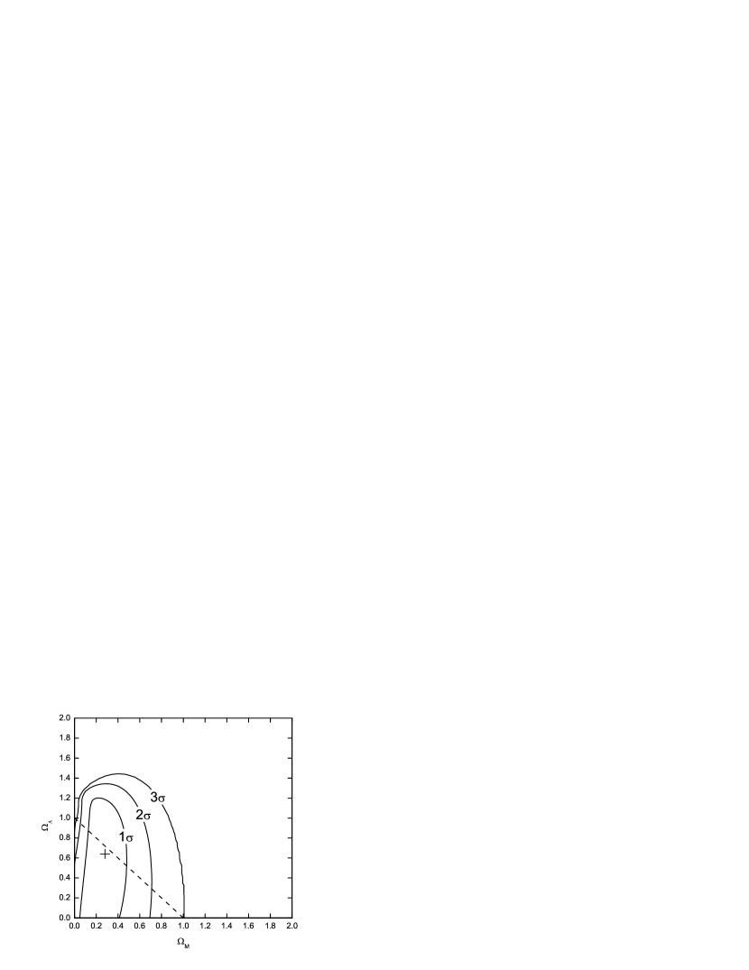
Figure 5.— The contours of likelihood interval distributions in the ($\Omega_{\rm{M}}$, $\Omega_{\Lambda}$)-plane inferred from the current GRB sample using the method developed in §4. The cross marks the most possible value of $(\Omega_{\rm{M}},\Omega_{\Lambda})$, which is $(0.28,0.64)$. The contours give $0.05<\Omega_{\rm{M}}<0.50$($1\sigma$). Considering a flat universe (the dashed line), the contours yield $0.13<\Omega_{\rm{M}}<0.49$ and $0.50<\Omega_{\Lambda}<0.85$ ($1\sigma$).

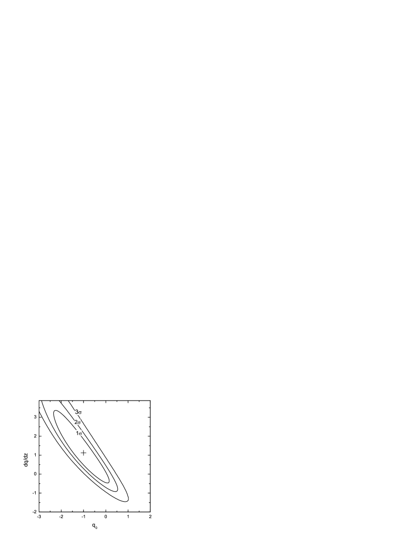
Figure 6.— The contours of likelihood interval distributions in the $(q_{0},dq/dz)$-plane inferred from the current GRB sample using the method developed in §4. The most possible values of $(q_{0},dq/dz)$ are $(-1.00,1.12)$ (the cross). At $1\sigma$ level their values are constrained in the ranges of $-2.23<q_{0}<0.26$ and $-0.07<dq/dz<3.48$, respectively.

Figure 7.— The smoothed likelihood function of the transition redshift from a decelerating Universe to an accelerating Universe inferred from the current GRB sample. The dashed lines mark the $1\sigma$ region, and the best value of $\hat{z}_{t}$ is $0.78^{+0.32}_{-0.23}$.

Figure 8.— The distributions of $z$, $E_{p}$, and $S_{\gamma}$ for the simulated GRB sample satisfying our model-independent standard candle relationship. For comparison, the imposed dotted lines are the distributions derived from the observational data.

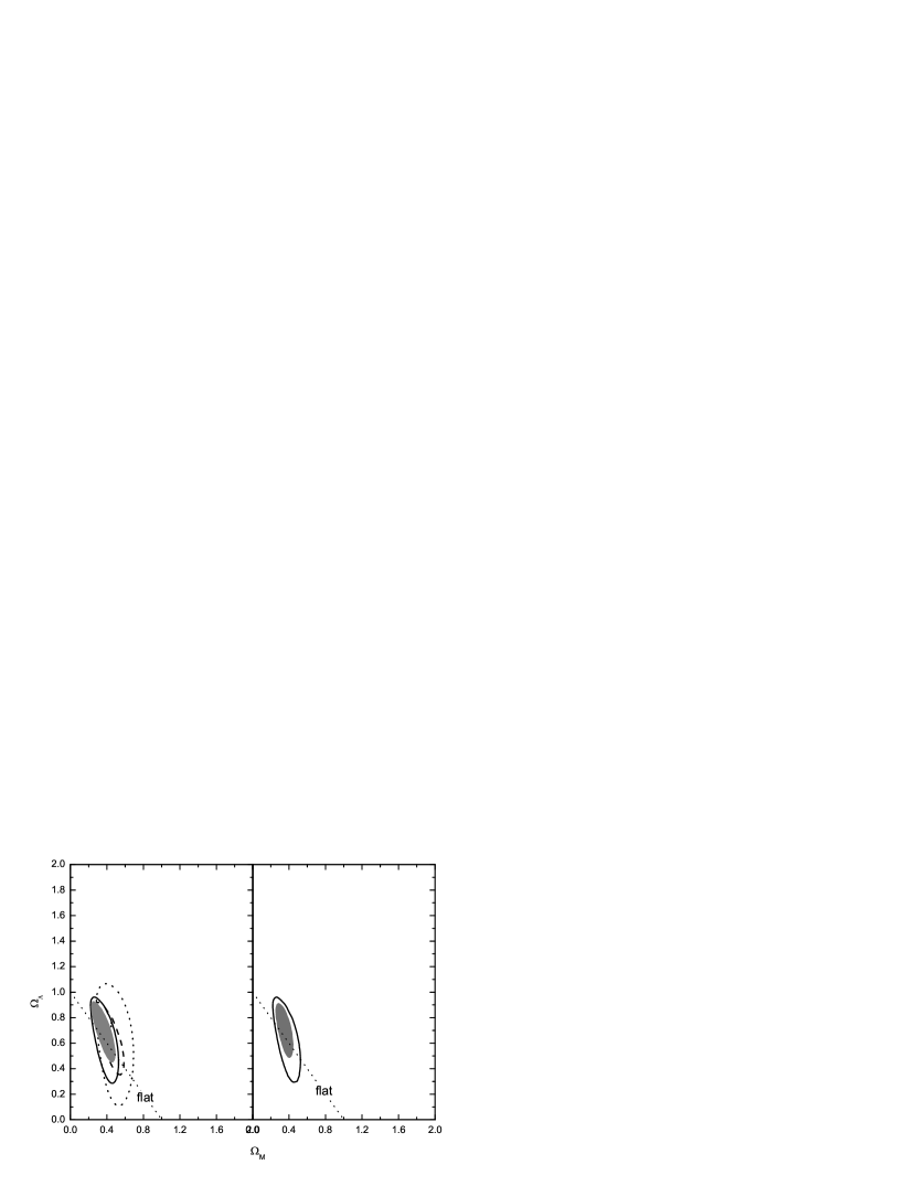
Figure 9.— A comparison of the $1\sigma$ likelihood contours for different simulated samples: right— Simulations for different sample sizes: dotted contour — 25 GRBs, solid contour — 50 GRBs, dashed contour — 75 GRBs, grey contour — 100 GRBs. The same observational errors ($\sigma_{x}/x=0.25k$, k is a random number between $0\sim 1$) are adopted; left: Simulations for a same sample size (50 GRBs) but for different observational errors: the line contour — $\sigma_{x}/x=0.25k$ and the grey contour— $\sigma_{x}/x=0.15k$ (see the procedure of our simulations). The dotted line is for a flat Universe.

Figure 10.— The contours of likelihood interval distributions in the ($\Omega_{\rm{M}}$, $\Omega_{\Lambda}$)-plane derived by the marginalization method. The cross marks the most possible value of $(\Omega_{\rm{M}},\Omega_{\Lambda})$ , which is $(0.28,0.52)$. The contours give $0.05<\Omega_{\rm{M}}<0.61$($1\sigma$). Considering a flat universe (the dashed line), the contours yield $0.14<\Omega_{\rm{M}}<0.58$ and $0.40<\Omega_{\Lambda}<0.84$ ($1\sigma$).

Figure 11.— Same as Fig. 5 but the uncertainties of the parameters in the empirical relationships are also included into the error of the distance modulus in the calculation of $p(\Omega)$ by Eq. 15. Only $1\sigma$ interval is shown.

Figure 12.— A demonstration of the potential constraints on cosmological parameters with high redshift GRBs. The gray contours are the results derived from 5 pseudo high redshift GRBs together with the observed GRB sample [$1\sigma$ (dark gray) to $3\sigma$ (light gray)], and the line contours are the results from the current observed GRB sample only.

References

- (1) Amati, L. 2004, astro-ph/0405318
- (2) Amati, L., et al. 2002, A&A, 390, 81
- (3) Andersen, M. I., et al. 2003, GCN, 1993
- (4) Band D. L., et al. 1993, ApJ, 413, 281
- (5) Band, D. L. & Preece , R. D. 2005, 627, ApJ, in press (astro-ph/0501559)
- (6) Barraud, C. et al. 2003, A&A, 400, 1021
- (7) Barth, A. J. et al. 2003, ApJ, 584, L47
- (8) Berger, E., et al. 2002, ApJ, 581, 981
- (9) Berger, E., et al. 2003, Nature, 426, 154
- (10) Björnsson, G., et al. 2001, ApJ, 552, L121
- (11) Bloom, J. S., Frail, D. A., & Kulkarni, S. R. 2003a, ApJ, 594, 674
- (12) Bloom, J. S., Morrell, N., & Mohanty, S. 2003b, GCN Report 2212
- (13) Bromm, V. & Loeb, A. 2002, ApJ, 575, 111
- (14) Butler, N. R., et al. 2003, GCN 2007
- (15) Ciardi, B. & Loeb, A. 2000, ApJ, 540, 687
- (16) Dai, Z. G. & Lu, T. 2002, ApJ, 580, 1013
- (17) Dai, Z. G., Liang, E. W., & Xu, D. 2004, ApJ, 612, L101
- (18) Djorgovski, S. G., et al. 2003, Proc. SPIE, 4834, astro-ph/0301342
- (19) Djorgovski, S. G., et al. 1999, GCN Report 510
- (20) Djorgovski, S. G., et al. 1998, ApJ, 508, L17
- (21) Eichler, D. & Levinson, A. 2004, preprint (astro-ph/0405014)
- (22) Fenimore, E. E. & Ramirez-Ruiz, E. 2000, astro-ph/0004176
- (23) Firmani, C., Ghisellini, G., Ghirlanda, G., & Avila-Reese, V., 2005, MNRAS, in press (astro-ph/0501395)
- (24) Frail, D. A., et al. 2001, ApJ, 562, L55
- (25) Frail, D. A., et al. 2003, ApJ, 590, 992
- (26) Friedmann, A. S. & Bloom, J. S. 2005, ApJ, in press
- (27) Galama, T. J., et al. 1999, GCN, 338
- (28) Gehrels, N., et al. 2004, ApJ, 611, 1005
- (29) Ghirlanda, G., Ghisellini, G., & Lazzati, D. 2004a, ApJ, 616, 331
- (30) Ghirlanda, G., et al. 2004b, ApJ, 613, L13
- (31) Gou, L. J., Mészáros, P., Abel, T., Zhang, B. 2004, ApJ, 604, 508
- (32) Greiner, J., Guenther, E., Klose, S., & Schwarz, R. 2003, GCN Report 1886
- (33) Halpern, J. P., et al. 2000, ApJ, 543, 697
- (34) Hjorth, J., et al. 2003, ApJ, 597, 699
- (35) Holland, S. T., et al. 2003, AJ, 125, 2291
- (36) Holland, S. T., et al. 2004, astro-ph/0405062
- (37) Holland, S. T., et al. 2002, AJ, 124, 639
- (38) Hurley, K., et al. 2000, GCN 529
- (39) Jakobsson, P., et al. 2003, A&A, 408, 941
- (40) Jakobsson, P., et al. 2004a, A&A, 427, 785
- (41) Jakobsson, P., et al. 2004b, ApJ, 617, L21
- (42) Jimenez, R., Band, D. L., & Piran, T., 2001, ApJ, 561, 171
- (43) Klose, S., et al. 2004, astro-ph/0408041
- (44) Kulkarni, S. R., et al. 1999, Nature, 398, 389
- (45) Lamb, D. Q., & Reichart, D. E. 2000, ApJ, 536, 1
- (46) Lamb, D. Q., et al. 2004, New Astronomy, 48, 423
- (47) Lamb, D. Q., Donaghy, T. Q., Graziani, C. 2005a, ApJ, 620, 355
- (48) Lamb, D. Q., et al. 2005b, astro-ph/0507362
- (49) Liang, E. W., Dai, Z. G., & Wu, X. F. 2004, ApJ, 606, L29
- (50) Lin, J. R., Zhang, S. N., & Li, T. P. 2004, ApJ, 605
- (51) Lloyd, N. M., Petrosian, V., & Mallozzi, R. S. 2000, ApJ, 534, 227
- (52) Lloyd-Ronning, N. M. & Zhang, B. 2004, 613,477
- (53) Möller, P., et al. 2002, A&A, 396, L21
- (54) MacFadyen, A. I. & Woosley, S. E. 1999, ApJ, 524, 262
- (55) Marshall, F. E. & Swank, J. H. 2003 GCN Reports 1996
- (56) Marshall, F. E., Markwardt, C., & Swank, J. H.,GCN 2052
- (57) Martini, P., Garnavich, P. & Stanek, K. Z. 2003, GCN Report 1980
- (58) Metzger, M. R., et al. 1997, Nature 387, 879
- (59) Mortsell, E. & Sollerman, J. 2005, preprint (astro-ph/0504245)
- (60) Nakar, E, & Piran, T. 2005, ApJ, submitted [astro-ph/0412232]
- (61) Norris, J. P., Marani, G. F., Bonnell, J. T. 2000, ApJ, 534, 248
- (62) Paczynski, B. 1998, ApJ, 494, L45
- (63) Panaitescu, A. & Kumar, P. 2002, ApJ, 571, 779
- (64) Pedersen, K., Fynbo, J., Hjorth, J., & Watson, D. 2003, GCN 1924
- (65) Perlmutter, S., et al. 1999, ApJ, 517, 565
- (66) Price, P. A., et al. 2003, ApJ, 589, 838
- (67) Qin Y. P., et al. 2005, preprint (astro-ph/0502373)
- (68) Ramirez-Ruiz, E., Lazzati, D., & Blain, A. W., 2002, ApJ, 565, L9
- (69) Rees, M. J. & Mészáros, P. 2005, ApJ, in press(astro-ph/0412702)
- (70) Reichart, D. E., et al. 2001, ApJ, 552, 57
- (71) Rhoads, J. E. 1999, ApJ, 525, 737
- (72) Riess, A. G., et al. 1998, AJ, 116, 1009
- (73) Riess, A. G., et al. 2004, ApJ, 607, 665
- (74) Rossi, E., Lazzati, D., Rees, M. J. 2002, MNRAS, 332, 945
- (75) Sakamoto, T. et al., 2004a, ApJ, 602, 875
- (76) Sakamoto, T. et al., 2004b, astro-ph/0409128
- (77) Salmonson, J. D.& Galama, T. J. 2002, ApJ,569, 682
- (78) Sari, R., Piran, T., & Halpern, J. P. 1999, ApJ, 519, L17
- (79) Schaefer, B. E. 2003, ApJ, 588, 387
- (80) Stanek, K. Z., et al. 1999, ApJ, 522, L39
- (81) Tiengo, A., Mereghetti, S.,& Schartel, N. 2003a, GCN 2241
- (82) Tiengo, A., Mereghetti, S.,& Schartel, N. 2003b, GCN 2285
- (83) Totani, T. 1997, ApJ, 486, L71
- (84) Vreeswijk, P. M., et al. 2001, ApJ, 546, 672
- (85) Vreeswijk, P., Fruchter, A., Hjorth, J., & Kouveliotou, C. 2003, GCN Report 1785
- (86) Weidinger, M., U, J. P., Hjorth, J., Gorosabel, J., Klose, S., & Tanvir, N. 2003, GCN Report 2215
- (87) Wu, X. F., Dai, Z. G., Liang, E. W. 2004, ApJ, 615, 359
- (88) Xu, D. 2005, preprint(astro-ph/0504052)
- (89) Xu, D., Dai, Z. G. & Liang. E. W., ApJ, submitted ,2005, astro-ph/0501458
- (90) Yamazaki, R., Ioka, K., & Nakamura, T. 2004, ApJ, 606, L33
- (91) Zhang, B. & Mészáros, P. 2002a, ApJ, 581, 1236
- (92) Zhang, B. & Mészáros, P. 2002b, ApJ, 571, 876